Exact mean field inference in asymmetric kinetic Ising systems

Abstract

We develop an elementary mean field approach for fully asymmetric kinetic Ising models, which can be applied to a single instance of the problem. In the case of the asymmetric SK model this method gives the exact values of the local magnetizations and the exact relation between equal-time and time-delayed correlations. It can also be used to solve efficiently the inverse problem, i.e. determine the couplings and local fields from a set of patterns, also in cases where the fields and couplings are time-dependent. This approach generalizes some recent attempts to solve this dynamical inference problem, which were valid in the limit of weak coupling. It provides the exact solution to the problem also in strongly coupled problems. This mean field inference can also be used as an efficient approximate method to infer the couplings and fields in problems which are not infinite range, for instance in diluted asymmetric spin glasses.

Inference problems are as old as scientific modelling: given data, how can we reconstruct a model which accounts for it, and find the parameters of the model? This is particularly difficult when data is obtained from networks of many interacting components. The fast development of high-throughput technologies in various fields of biology, ranging from gene regulation to protein interaction and neural activity, is generating a lot of data, which is challenging our ability to infer the structure and parameters of the underlying networks.

This ‘network reconstruction’ problem is typically an inverse problem which has motivated a lot of activity in machine learning and in statistical physicsAckleyHinton ; Hinton ; KappenSpanjers ; KappenRodriguez ; Tanaka ; SessakMonasson ; MezardMora ; Marinari ; HuangSuscProp ; HuangMF ; Wainwright ; AurellOR ; HertzRTTAZ ; RoudiHertzPRL ; RoudiHertzLong ; RoudiAH ; ZengAAM ; WeigtWhite ; BraunsteinPWZ ; CoccoLeibMon . Until recently the main efforts have been dedicated to reconstructing equilibrium Boltzmann-Gibbs distributions. In the so-called inverse Ising model, one typically assumes to have data in the form of some configurations, which we shall call ‘patterns’, of a $N$-spin Ising system drawn from the Boltzmann-Gibbs distribution with an energy function including one-body (local magnetic fields) and two-body (exchange couplings) terms. The problem is to reconstruct the local fields and the exchange couplings (collectively denoted below as ‘couplings’) from the data. This problem has been actively studied in recent years, in particular in the context of neural network inference based on multielectrode recordings in retinas SchneidBSB ; ShlensFGG ; CoccoLeibMon . The standard solution of this problem, known as the Boltzmann machine, computes, for some given couplings, the local magnetizations and the two-spin correlations, and compares them to the empirical estimates of magnetizations and correlations found from the patternsAckleyHinton ; Hinton . The couplings are then iteratively adjusted in order to decrease the distance between the empirical magnetizations/correlations and the ones computed from the model. A Bayesian formulation shows that the problem of finding the couplings is actually convex, so that this iterative procedure is guaranteed to converge to the correct couplings, provided that the number of patterns is large enough to allow for a good estimate of correlations. The drawback of this method is that the reliable computation of the magnetizations/correlations, given the couplings, which is done using a Monte Carlo procedure, is extremely time consuming. Therefore this exact approach is limited to systems with a small number of spins. Most of the recent works on this issue have developed approximate methods to infer the couplings. Among the most studied approaches are the naive mean field method KappenRodriguez ; Tanaka ; HertzRTTAZ , the TAP approach KappenSpanjers ; RoudiHertzPRL ; ZengAAM , a method based on a small magnetization expansion SessakMonasson , and a message-passing method called susceptibility propagationMezardMora ; Marinari ; HuangSuscProp . Another approach which has been developed is that of linear relaxation of the inference problemWainwright . The inverse-Potts problem is a version of this same problem, with variables taking $q$ possible states. The case $q=20$ is relevant for inferring interaction in protein pairs from data on co-evolution of these pairs, and its solution by susceptibility propagation has given an accurate prediction of inter-protein residue contactsWeigtWhite . Another case which has received some attention is the problem of reconstruction in Boolean networks (see e.g.BraunsteinPWZ and references therein).

However, in many applications to biological systems, in particular the ones concerning neural activity and gene expression network, the assumption that the patterns are generated by an underlying equilibrium Boltzmann-Gibbs measure is not well founded. Couplings are typically asymmetric, and they may vary in time, so there is no equilibrium measure. This has prompted the recent study of inference in purely kinetic models without an equilibrium measure CoccoLeibMon ; HertzRTTAZ ; RoudiHertzPRL ; ZengAAM . A benchmark on this dynamic inference problem is the inverse asymmetric kinetic Ising model. The framework is the same as the equilibrium one: one tries to infer the parameters of the dynamical evolution equation of an Ising spin systems, given a set of patterns generated by this evolution. The recent works HertzRTTAZ ; RoudiHertzPRL ; RoudiHertzLong ; ZengAAM have studied the performance of two mean-field methods on this problem, the naive mean field (nMF) and a weak-coupling expansion which they denote as TAP method. They have shown that, in the case of the fully asymmetric infinite range spin glass problem, the inference problem can be solved by these methods in the case where the spins are weakly coupled. In the present work we present a (non-naive!) mean field approach which solves the problem at all values of the couplings (and reduces to their TAP approach at weak coupling).

Figure 1: Magnetizations (left column) and correlations (right column) obtained by MF (blue), ‘TAP’ (green) and nMF (red). One $N=200$ spin model is simulated $500000$ times for $31$ time steps. The three plots in each column correspond to inverse temperature $\beta=.3,\;.8$ and $1.4$ (from top to bottom). In the left column, the magnetizations predicted by each method for all time steps are plotted versus the experimental ones found by monte carlo simulation. For the plots of the right column, the correlation matrices $C$ and $D$ are obtained at $t=30$. The scatter plot shows for each pair $ij$, the value of $D_{ij}$ in ordinate, and the value of $(AJC)_{ij}$ in abscissa. The three methods differ in their predictions for $A$. At high temperature, $\beta=.3$, all methods are good for both the magnetizations and correlations; the MF and ‘TAP’ methods nearly coincide and are slightly better than nMF. At larger and larger $\beta$, the ‘TAP’ correction to naive mean field overshoots, and only the MF results is correct. The data supports the statement that MF is exact at all temperatures, while nMF and ‘TAP’ are only high temperature approximations.

The kinetic Ising model which we shall study is the same as the one of RoudiHertzPRL . $N$ Ising spins $s_{i}$ evolve in discrete time, with a synchronous parallel dynamics. Given the configuration of spins at time $t-1$, $s(t-1)=\{s_{1}(t-1),\dots,s_{N}(t-1)\}$, the spins $s_{i}(t)$ are independent random variables drawn from the distribution:

$$P(s(t)|s(t-1))=\prod_{i=1}^{N}\frac{1}{2\cosh(\beta h_{i}(t))}e^{\beta s_{i}(t)h_{i}(t)}$$ (1)

where

$$h_{i}(t)=H_{i}(t-1)+\sum_{j}J_{ij}(t-1)s_{j}(t-1)$$ (2)

Note that both the local external fields $H_{i}(t)$ and the exchange couplings $J_{ij}(t)$ may depend on time. Here we are interested in a fully asymmetric model. We generate the $J_{ij}$ by an asymmetric version HertzGS ; Parisi ; Derrida of the infinite -range Sherrington-Kirkpatrick spin glass model SK , in which for each directed edge $(ij)$ the coupling is a gaussian random variable with variance $1/N$. Notice that $J_{ij}$ and $J_{ji}$ are independent random variables. We do not include self-interactions (we take $J_{ii}=0$), although this could be done without changing the results. As initial conditions we take $s_{i}(t=0)=\pm 1$ with probability $1/2$. Our method also applies to the case of asynchronous dynamics, studied in ZengAAM with the TAP approach, but to keep the presentation simple we shall study only the case of the synchronous parallel dynamics in this letter.

We first derive the mean-field equations for the magnetizations $m_{i}(t)=\langle s_{i}(t)\rangle$. Because the couplings are asymmetric, $\sum_{j}J_{ij}J_{ji}=O(1/\sqrt{N})$, therefore the Onsager reaction term is not present in this problem. This makes the derivation of our equations, which we shall denote just ’mean-field’ equations, particularly easy. The approximate equations used in RoudiHertzPRL ; ZengAAM , originally derived in KappenRodriguez , have been obtained by a second order expansion in the couplings. When this expansion is applied to the symmetric problem it gives back the TAP equations TAP with their Onsager reaction term. In the present case of asymmetric coupling, it keeps the correction of order $\sum_{j}J_{ij}J_{ij}$. We shall keep for these second-order-expanded equations the name ‘TAP’-equations, as used by KappenRodriguez ; RoudiHertzPRL ; ZengAAM .

The local field on spin $i$ due to the other spins, $\sum_{j}J_{ij}(t-1)s_{j}(t-1)$, is the sum of a large number of terms. Therefore it has a gaussian distribution with mean

$$g_{i}(t-1)=\sum_{j}J_{ij}m_{j}(t-1)$$ (3)

and variance

$$\Delta_{i}(t-1)=\sum_{j}J_{ij}^{2}(1-m_{j}(t-1)^{2})$$ (4)

(in order to derive this last formula, one must use the fact that the typical connected correlation $\langle s_{j}s_{k}\rangle-m_{j}m_{k}$ is typically of order $1/\sqrt{N}$; this will be checked self-consistently below). Using this property and the definition of the dynamics (1), one obtains the magnetization of spin $i$ at time $t$:

$$m_{i}(t)=\int Dx\;\tanh\left[\beta\left(H_{i}(t-1)+g_{i}(t-1)+x\sqrt{\Delta_{i}(t-1)}\right)\right]\ ,$$ (5)

where $Dx=\frac{dx}{\sqrt{2\pi}}\text{e}^{-\frac{x^{2}}{2}}$ is the probability density for a Gaussian variable $x$ with zero mean and variance unity.

Equations (3,4,5) are our mean field (MF) equations for this problem, valid on a given instance. Similar dynamical equations have been obtained in the study of the sample-averaged order parameter in asymmetric neural networksDerGarZip ; GutMez and spin glassesDerrida . They can be iterated starting from some initial condition (in our case $m_{i}(0)=0$) in order to get all the magnetizations $m_{i}(t)$ at any time. They rely only on the central limit theorem and they are exact in the large $N$ limit, for any set of couplings and external fields, even if they are time-dependent. These differ from the ‘TAP’ equations of RoudiHertzPRL ; ZengAAM ; KappenRodriguez ; KappenSpanjers which can be written in our notation:

$$m_{i}(t)=\tanh\left[\beta H_{i}(t-1)+\beta g_{i}(t-1)-m_{i}(t)\beta^{2}\Delta_{i}(t-1)\right]\ ,$$ (6)

and from the naive mean field (nMF) equations:

$$m_{i}(t)=\tanh\left[\beta\left(H_{i}(t-1)+g_{i}(t-1)\right)\right]\ .$$ (7)

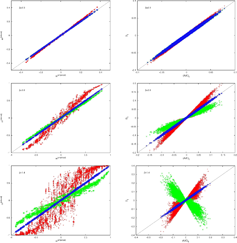
The nMF equations and the ‘TAP’ equations actually give the same result as our exact MF equations, when expanded in powers of $\Delta_{i}$, respectively to order $\Delta_{i}^{0}$ and $\Delta_{i}^{1}$, but they differ at order $\Delta_{i}^{2}$. The fact that ‘TAP’ equations agree with the exact MF to second order in a weak coupling expansion is consistent with their derivation through second order Plefka-type expansionKappenSpanjers . The correctness of the MF equations (5,3,4) can be easily checked numerically as shown in the left panels of Fig.1.

We now turn to the computation of correlations. We shall establish the mean field relation between the time-delayed and the equal-time correlation matrices:

$$D_{ij}(t) \equiv \langle\delta s_{i}(t+1)\delta s_{j}(t)\rangle$$ (8)

$$C_{ij}(t) \equiv \langle\delta s_{i}(t)\delta s_{j}(t)\rangle\ ,$$ (9)

where we define $\delta s_{i}(t)$ as the fluctuation of the magnetization: $\delta s_{i}(t)=s_{i}(t)-\langle s_{i}(t)\rangle\ .$

We start by writing $\sum_{j}J_{ij}(t)s_{j}(t)=g_{i}(t)+\delta g_{i}(t)$, where ${\delta g_{i}}(t)$ is gaussian distributed with mean $0$ and variance $\Delta_{i}(t)$. Now, by definition of $D_{ij}$ we have

$$D_{ij}(t)=\langle s_{j}(t)\tanh\left[\beta\left(H_{i}(t)+g_{i}(t)+{\delta g_{i}}(t)\right)\right]\rangle-\langle s_{j}(t)\rangle\langle\tanh\left[\beta\left(H_{i}(t)+g_{i}(t)+{\delta g_{i}}(t)\right)\right]\rangle$$ (10)

Hereafter in order to keep notations simple in the derivation of the relation between $D(t)$ and $C(t)$ we work at a fixed time $t$ and we thus drop the explicit time indices: all time indices in this derivation are equal to $t$ (e.g. $J_{ij}=J_{ij}(t)$, $\delta s_{i}=\delta s_{i}(t)$, $g_{i}=g_{i}(t)$ etc.) We get:

$$\begin{split}\sum_{k}J_{jk}D_{ik}&=\langle\left(g_{j}+\delta g_{j}\right)\tanh\left[\beta\left(H_{i}+g_{i}+\delta g_{i}\right)\right]\rangle-g_{j}\langle\tanh\left[\beta\left(H_{i}+g_{i}+\delta g_{i}\right)\right]\rangle\\ &=\langle\delta g_{j}\tanh\left[\beta\left(H_{i}+g_{i}+\delta g_{i}\right)\right]\rangle\end{split}$$ (11)

In order to evaluate the average we need the joint distribution of $\delta g_{i}$ and $\delta g_{j}$. The crucial point to keep in mind is that, as the couplings are of order $1/\sqrt{N}$, each matrix element of $C$ and $D$ is also small, of order $1/\sqrt{N}$. Their covariance is therefore small:

$$\langle\delta g_{i}\delta g_{j}\rangle = \langle\sum_{k}J_{ik}\left(s_{k}-\langle s_{k}\rangle\right)\sum_{l}J_{jl}\left(s_{l}-\langle s_{l}\rangle\right)\rangle$$ (12)

$$= \sum_{k,l}J_{ik}J_{jl}C_{kl}=\left(JCJ^{T}\right)_{ij}\equiv\varepsilon\ ,$$ (13)

where $\varepsilon$ is typically of order $1/\sqrt{N}$. So the joint distribution of $x=\delta g_{i}$ and $y=\delta g_{j}$ takes the form, in the large $N$ limit (omitting terms of order $\varepsilon^{2}$):

$$P(x,y)=\frac{1}{2\pi\sqrt{\Delta_{i}\Delta_{j}}}\exp\left(-\frac{x^{2}}{2\Delta_{i}}-\frac{y^{2}}{2\Delta_{j}}+\varepsilon\frac{xy}{\Delta_{i}\Delta_{j}}\right)$$ (14)

Using the small $\varepsilon$ expansion of eq. (14) we can rewrite eq. (11) as

$$\sum_{k}J_{jk}D_{ik} = \frac{\varepsilon}{\Delta_{i}\Delta_{j}}\int\frac{dx}{\sqrt{2\pi\Delta_{i}}}\frac{dy}{\sqrt{2\pi\Delta_{j}}}\text{e}^{-\frac{x^{2}}{2\Delta_{i}}-\frac{y^{2}}{2\Delta_{j}}}xy^{2}\tanh\left[\beta\left(H_{i}+g_{i}+x\right)\right]$$ (15)

$$= \varepsilon\beta\int\frac{dx}{\sqrt{2\pi\Delta_{i}}}\exp^{-\frac{x^{2}}{2\Delta_{i}}}\left(1-\tanh^{2}\left[\beta\left(H_{i}+g_{i}+x\right)\right]\right)\ .$$ (16)

Combining eq. (12) and eq. (15) we get:

$$\left(DJ^{T}\right)_{ij}=\left(JCJ^{T}\right)_{ij}\beta\int\frac{dx}{\sqrt{2\pi\Delta_{i}}}\text{e}^{-\frac{x^{2}}{2\Delta_{i}}}\left(1-\tanh^{2}\beta\left(H_{i}+g_{i}+x\right)\right)\ ,$$ (17)

which gives the explicit mean-field relation between $C$ and $D$. Putting back the time indices, we obtain the final result in matrix form:

$$D(t)=A(t)\;J(t)\;C(t)\ ,$$ (18)

where $A(t)$ is a diagonal matrix: $A_{ij}(t)=a_{i}(t)\delta_{ij}$, with:

$$a_{i}(t)=\beta\int Dx\;\left[1-\tanh^{2}\beta\left(H_{i}(t)+g_{i}(t)+x\sqrt{\Delta_{i}(t)}\right)\right]\ .$$ (19)

The final result (18) takes exactly the same form as the one found with the naive mean field equation and with the ‘TAP’ approach. The predictions of all three methods, nMF, ‘TAP’ and our MF method is always $D(t)=A(t)\;J(t)\;C(t)$, with a diagonal matrix $A(t)$ which differs in each case. As shown in RoudiHertzPRL , the nMF approximation gives:

$$a_{i}^{nMF}(t)=\beta\left[1-m_{i}(t+1)^{2}\right]\ ,$$ (20)

the ‘TAP’ approximation gives:

$$a_{i}^{TAP}(t+1)=\beta\left[1-m_{i}(t+1)^{2}\right]\left[1-(1-m_{i}(t+1)^{2})\beta^{2}\sum_{k}J_{ik}^{2}(1-m_{k}(t)^{2})\right]$$ (21)

and our mean field prediction is the one given in (19).

We claim that, as in the case of the magnetizations, our mean field equations connecting $D$ to $C$ are exact in the asymmetric SK model, in the large $N$ limit. This statement can be checked numerically by comparing $(AJC)_{ij}$ with the experimental values of $D_{ij}$ found by monte carlo simulations, as shown in Fig.1.

Figure 2: Left: The infered couplings found by MF (blue), ‘TAP’ (green) and nMF (red) plotted versus the real ones for a $N=100$ model, given $P=1000000$ patterns generated at inverse temperature $\beta=0.4$. Right: The same for $\beta=1.4$ (MF (blue) and nMF (red), ‘TAP’ is not shown as it fails at this high $\beta$)

Figure 3: Mean square error of the infered couplings $\overline{(J_{ij}^{\text{infered}}-J_{ij}^{\text{real}})^{2}}$ obtained by MF inference (blue), ‘TAP’ (green) and nMF (red) versus the number of patterns used to estimate the correlations, for a system of size $N=40$, where the patterns were generated from a gaussian distribution with a root-mean-square $\beta=0.2$ (left) and $\beta=0.6$ (right). The curves are averages performed over $20$ realizations of the couplings and fields. Notice that the ‘TAP’ method is absent in the right figure because it fails to provide results at strong coupling.

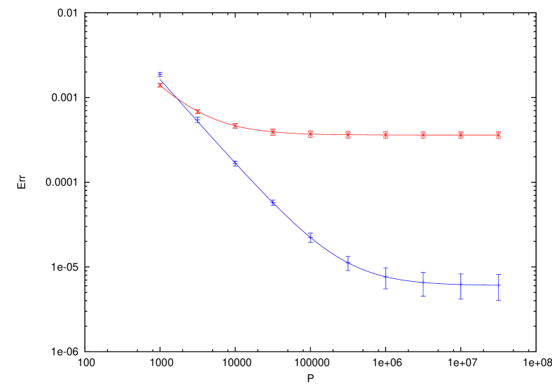
These results on the mean field relation between $C$ and $D$ can be used for the inverse problem. Given $P$ ‘patterns’, which are time sequences of length $t$ generated from the distribution (1), one can estimate for each $\tau=1,\dots,t$, the magnetizations $m_{i}(\tau)$, the equal time correlations $C_{ij}(\tau)$ and the time-delayed correlations $D_{ij}(\tau)$. The problem is to infer from these data the values of the couplings $J_{ij}(\tau)$ and of the local fields $H_{i}(\tau)$. Without loss of generality, we can use $\beta=1$ as it is absorbed in the strength of couplings and fields that we want to infer. We shall solve this problem using the mean field equations.

The problems corresponding to different times and sites decouple. So let us consider a fixed value of $i$ and $\tau$, and infer the $J_{ij}(\tau)$ for $j=1,\dots,N$, and $H_{i}(\tau)$. To lighten notation we drop the explicit indices $\tau$ and $i$, and we denote $H=H_{i}(\tau)$, $m_{j}=m_{j}(\tau)$, $m=m_{i}(\tau+1)$, $g=g_{i}(\tau)$, $\Delta=\Delta_{i}(\tau)$, $a=a_{i}(\tau)$. Following RoudiHertzPRL , one can obtain $J$ by inverting the relation (18). The first step is to invert the empirical $C$ matrix and compute:

$$b_{j}=\sum_{k}D_{ik}(\tau)C^{-1}_{kj}(\tau)\ .$$ (22)

If one knows the number $a=a_{i}(\tau)$ one can then infer the couplings from (18):

$$J_{ij}(\tau)=b_{j}/a\ .$$ (23)

Let us now see how $a$ can be computed. The mean field equation (5) for the magnetization reads:

$$m=\int Dx\;\tanh\left[H+g+x\sqrt{\Delta}\right]\ .$$ (24)

The equation (19) for $a$ is

$$a=\int Dx\left(1-\tanh^{2}\left[H+g+x\sqrt{\Delta}\right]\right)\ .$$ (25)

The link between $a$ and $\Delta$ is obtained from (4), which reads:

$$\Delta=\frac{1}{a^{2}}\sum_{j}b_{j}^{2}(1-m_{j}^{2})=\frac{\gamma}{a^{2}}\ .$$ (26)

To solve this system of equations, we propose the following iterative procedure. Using the empirical correlations and magnetizations estimated from the patterns, we first compute from (22) the $\{b_{j}\}$, $j\in\{1,\dots,N\}$, and $\gamma=\sum_{j}b_{j}^{2}(1-m_{j}^{2})$.

Then we use the following mapping to find $\Delta$.

• Start from a given value of $\Delta$.

• Using the empirical value of $m$ and the value of $\Delta$, compute $H+g$ by inverting (24). The right-hand side of this equation is an increasing function of $H+g$ so this inversion is easy.

• Using $H+g$ and $\Delta$, compute $a$ using (25)

• Compute the new value of $\Delta$, called $\hat{\Delta}$, using (26).

It is worth pointing out that in the thermodynamic limit, $N\to\infty$, the value of $\Delta$ becomes independent of $i$. So, if the system under consideration is large enough, the above iteration could be perfomed only once in order to reduce computation time.

This procedure defines a mapping from $\Delta$ to $\hat{\Delta}=f(\Delta)$, and we want to find a fixed point of this mapping. It turns out that a simple iterative procedure, starting from an arbitrary $\Delta_{0}$ (for instance $\Delta_{0}=1$) and using $\Delta_{n+1}=f(\Delta_{n})$, usuallly converges. More precisely, it can be shown that $f(0)=\frac{\gamma}{(1-m^{2})^{2}}$ and that the asymptotic form for the slope of $f$ for $\Delta\gg 1$ is $f^{\prime}\sim\frac{\pi}{2}\gamma\text{exp}(\hat{u}^{2})\Delta_{n}$, where $\hat{u}$ is such that $m=\text{erf}(\hat{u}/\sqrt{2})$. We have found numerically that when the number of patterns is large enough the slope verifies: $df/d\Delta\in]0,1[$. Therefore the mapping converges exponentially fast to the unique fixed point. This method therefore works when the number of patterns per spin $P/N$ is large enough. In the double limit $P,N\to\infty$ and $P/N$ large enough the above procedure thus allows to get the exact result for $\Delta$; and therefore to find the couplings $J_{ij}(\tau)=b_{j}/a$. Once the couplings have been found, one can easily compute $g=\sum_{j}J_{ij}(\tau)m_{j}(\tau)$, and therefore get the local field $H(\tau)$. The number of operations needed for the full inference of the couplings and fields is dominated by the inversion of the correlation matrix $C$, a time which is typically at most of order $N^{3}$. If the number of patterns is too small, it may happen that there is no solution to the fixed point equation $f(\Delta)=\Delta$. Then one can decide to use $\Delta=f(0)$, which is nothing but the nMF estimate for $a_{i}(\tau)$.

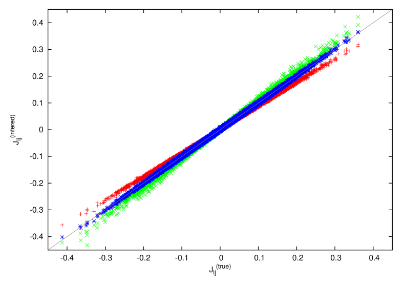
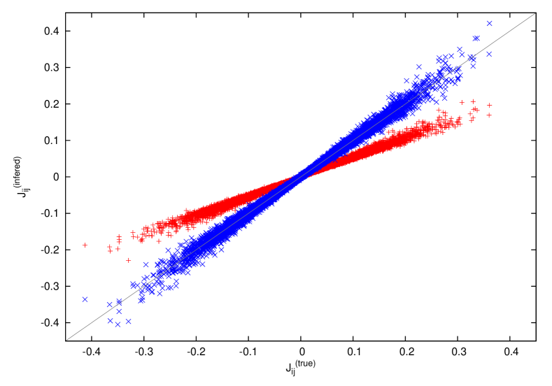
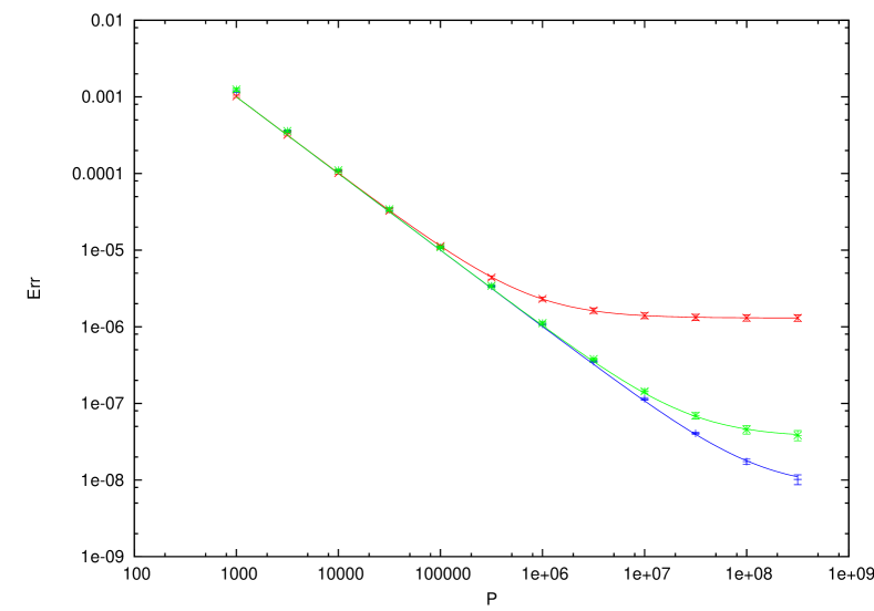
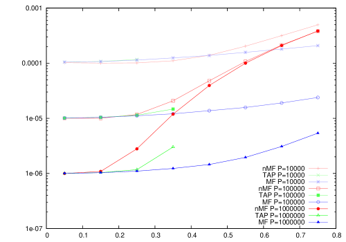
We have tested our mean field inference method on the asymmetric SK problem, where the couplings $J_{ij}$ are time-independent, gaussian distributed with variance $\beta^{2}$ and the fields are time independent, uniformly distributed on $[-\beta,\beta]$ . Fig.(2) shows a scatter plot of the result on one given instance at $\beta=.4$ and $\beta=1.4$, and compares it to the inference method of RoudiHertzPRL using nMF and ‘TAP’ (the ‘TAP’ inference is limited to small values of $\beta$: at large $\beta$ it fails). Figs. 3 and 4 show a statistical analysis of the performance of MF inference. It accurately infers the couplings and fields even in the strong coupling regime.

Figure 4: Mean square error of the reconstructed couplings versus $\beta$, averaged over $10$ systems with $100$ spins, using the three inference methods nMF, ‘TAP’ and MF, with a number of patterns $P=10000$, $P=100000$ and $P=1000000$. All three methods agree at small $\beta$. The nMF error can increase by several orders of magnitude at large $\beta$. The ‘TAP’ method fails to provide results above $\beta\approx 0.4$. The MF inference method gives good results in the whole range of $\beta$.

Figure 5: Mean field inference of a finite connectivity model. The couplings found by MF (blue) and nMF (red) are plotted versus the real couplings used to generate the data for a $N=200$ model on an asymmetric random regular graph with connectivity $c=6$ (average in-degree=$3$) , given $P=100000$ patterns generated at inverse temperature $\beta=.6$.

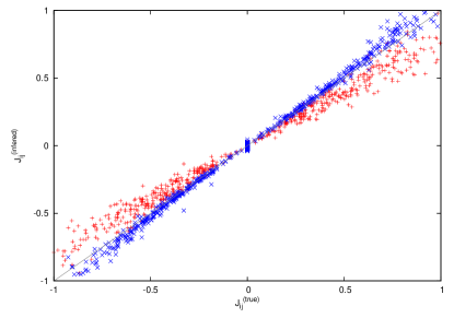
The method that we propose is exact and allows for a very precise inference of the couplings when applied to the fully asymmetric SK spin glass, at any temperature, if the number of patterns is large enough. At the same time, it is an easy and versatile method which can be used as an approximate inference method when the number of patterns is not very large (although one should at least have $P>N$ in order for $C$ to be invertible), or when the underlying model is not of the SK type. As an example showing the possible use of the method, we have applied it to a sample where the $J_{ij}$ matrix is sparse, generated as follows. We first generate a regular graph with $200$ vertices and degree $6$ on each vertex. For each edge $ij$ of this graph we choose randomly with probability $1/2$ an orientation, say $i\to j$. Then we take $J_{ji}=0$ and $J_{ij}$ is drawn randomly from the probability density $(|x|/2)e^{-x^{2}/2}$. All the other couplings corresponding to pairs of sites $kl$ which are not in the graph are set to $0$. One then iterates the dynamics (1) 100000 times at $\beta=.6$, and uses this data to reconstruct the couplings. Fig. 5 shows the resulting couplings as a scatter plot. The topology of the underlying interaction graph can be reconstructed basically exactly, both by nMF and MF by using a threshold, deciding that all reconstructed couplings with $|J_{ij}|<.04$ vanish. The non-zero couplings are found accurately by the MF inference method.

To summarize, we have introduced a simple mean field method which can be applied on a single instance of a dynamical fully asymmetric Ising model. In the case of the asymmetric SK model this MF method gives the exact values of the local magnetizations and the exact relation between equal-time and time-delayed correlations. This method can be used to solve efficiently the inverse problem, i.e. determine the couplings and local fields from a set of patterns. Again this inference method is exact in the limit of large sizes and large number of patterns, in the asymmetric SK case. It can also be used in cases where the underlying model is different, for instance for diluted models. This could be quite useful for many applications.

We thank Lenka Zdeborová for useful discussions.This work has been supported in part by the EC grant ’STAMINA’, No 265496.

References

- [1] David H. Ackley, Geoffrey E. Hinton, and Terrence J. Sejnowski. A learning algorithm for Boltzmann machines. Cognitive Science, 9(1):147–169, 1985.
- [2] E. Aurell, C. Ollion, and Y. Roudi. Dynamics and performance of susceptibility propagation on synthetic data. The European Physical Journal B - Condensed Matter and Complex Systems, 77:587–595, 2010. 10.1140/epjb/e2010-00277-0.
- [3] A Braunstein, A Pagnani, M Weigt, and R Zecchina. Gene-network inference by message passing. Journal of Physics: Conference Series, 95(1):012016, 2008.
- [4] Simona Cocco, Stanislas Leibler, and Rémi Monasson. Neuronal couplings between retinal ganglion cells inferred by efficient inverse statistical physics methods. Proceedings of the National Academy of Sciences, 106(33):14058–14062, 2009.
- [5] B. Derrida. Dynamical phase transition in non-symmetric spin glasses. J. Phys. A, 20:L721–L725, 1987.
- [6] B. Derrida, E. Garner, and A. Zippelius. An exactly solvable asymmetric neural network model. Europhys. Lett., 4:167–173, 1987.
- [7] H. Gutfreund and M. Mézard. Processing of temporal sequences in neural networks. Phys. Rev. Lett., 61:235–238, 1988.
- [8] J. Hertz, G. Grinstein, and S. Solla. Irreversible spin glasses and neural networks. In J. van Hemmen and I. Morgenstern, editors, Heidelberg Colloquium on Glassy Dynamics, volume 275 of Lecture Notes in Physics, pages 538–546. Springer Berlin / Heidelberg, 1987. 10.1007/BFb0057533.
- [9] John Hertz, Yasser Roudi, Andreas Thorning, Joanna Tyrcha, Erik Aurell, and Hong-Li Zeng. Inferring network connectivity using kinetic ising models. BMC Neuroscience, 11(Suppl 1):P51, 2010.
- [10] Geoffrey E. Hinton. Deterministic boltzmann learning performs steepest descent in weight-space. Neural Computation, 1(1):143–150, 1989.
- [11] Haiping Huang. Message passing algorithms for the hopfield network reconstruction: Threshold behavior and limitation. Phys. Rev. E, 82(5):056111, Nov 2010.
- [12] Haiping Huang. Reconstructing the hopfield network as an inverse ising problem. Phys. Rev. E, 81(3):036104, Mar 2010.
- [13] H. J. Kappen and F. B. Rodríguez. Efficient learning in boltzmann machines using linear response theory. Neural Computation, 10(5):1137–1156, 1998.
- [14] H. J. Kappen and J. J. Spanjers. Mean field theory for asymmetric neural networks. Phys. Rev. E, 61(5):5658–5663, May 2000.
- [15] Enzo Marinari and Valery Van Kerrebroeck. Intrinsic limitations of the susceptibility propagation inverse inference for the mean field ising spin glass. Journal of Statistical Mechanics: Theory and Experiment, 2010(02):P02008, 2010.
- [16] Marc Mézard and Thierry Mora. Constraint satisfaction problems and neural networks: A statistical physics perspective. Journal of Physiology-Paris, 103(1-2):107 – 113, 2009. Neuromathematics of Vision.
- [17] G. Parisi. Asymmetric neural networks and the process of learning. Journal of Physics A Mathematical General, 19:L675–L680, August 1986.
- [18] P. Ravikumar, M. J. Wainwright, and J. D. Lafferty. High-dimensional Ising model selection using $ell_1$-regularized logistic regression. ArXiv e-prints, October 2010.
- [19] Yasser Roudi, Erik Aurell, and John Hertz. Statistical physics of pairwise probability models. ArXiv e-prints, 2009.
- [20] Yasser Roudi and John Hertz. Dynamical tap equations for non-equilibrium ising spin glasses. ArXiv e-prints, 2011.
- [21] Yasser Roudi and John Hertz. Mean field theory for nonequilibrium network reconstruction. Phys. Rev. Lett., 106(4):048702, Jan 2011.
- [22] Elad Schneidman, Michael J. Berry, Ronen Segev, and William Bialek. Weak pairwise correlations imply strongly correlated network states in a neural population. Nature, 440(7087):1007–1012, April 2006.
- [23] Vitor Sessak and Rémi Monasson. Small-correlation expansions for the inverse ising problem. ArXiv e-prints, 2008.
- [24] David Sherrington and Scott Kirkpatrick. Solvable model of a spin-glass. Phys. Rev. Lett., 35(26):1792–1796, Dec 1975.
- [25] Jonathon Shlens, Greg D. Field, Jeffrey L. Gauthier, Matthew I. Grivich, Dumitru Petrusca, Alexander Sher, Alan M. Litke, and E. J. Chichilnisky. The structure of multi-neuron firing patterns in primate retina. The Journal of Neuroscience, 26(32):8254–8266, 2006.
- [26] Toshiyuki Tanaka. Mean-field theory of boltzmann machine learning. Phys. Rev. E, 58(2):2302–2310, Aug 1998.
- [27] D. J. Thouless, P. W. Anderson, and R. G. Palmer. Solution of ’solvable model of a spin glass’. Philosophical Magazine, 35:593–601, 1977.
- [28] Martin Weigt, Robert A. White, Hendrik Szurmant, James A. Hoch, and Terence Hwa. Identification of direct residue contacts in protein–protein interaction by message passing. Proceedings of the National Academy of Sciences, 106(1):67–72, 2009.
- [29] H.-L. Zeng, E. Aurell, M. Alava, and H. Mahmoudi. Network inference using asynchronously updated kinetic Ising Model. ArXiv e-prints, November 2010.