Conserved Density Fluctuation and Temporal Correlation Function in HTL Perturbation Theory

Abstract

Considering recently developed Hard Thermal Loop perturbation theory that takes into account the effect of the variation of the external field through the fluctuations of a conserved quantity we calculate the temporal component of the Euclidian correlation function in the vector channel. The results are found to be in good agreement with the very recent results obtained within the quenched approximation of QCD and small values of the quark mass ($\sim 0.1T$) on improved lattices of size $128^{3}\times N_{\tau}$ at ($N_{\tau}=40,\ T=1.2T_{C}$), ($N_{\tau}=48,\ T=1.45T_{C}$), and ($N_{\tau}=16,\ T=2.98T_{C}$), where $N_{\tau}$ is the temporal extent of the lattice. This suggests that the results from lattice QCD and Hard Thermal Loop perturbation theory are in close proximity for a quantity associated with the conserved density fluctuation.

I Introduction

Dynamical properties of many particle system can generally be studied by employing an external perturbation, which disturbs the system only slightly from its equilibrium state, and thus measuring the spontaneous response/fluctuations of the system to this external perturbation. In general, the fluctuations are related to the correlation function through the symmetry of the system, which provides important inputs for quantitative calculations of complicated many-body system. Also, many of the properties of the deconfined strongly interacting matter are reflected in the structure of the correlation and the spectral functions hasimoto of the vector current.

The static thermal dilepton rate describing the production of lepton pairs is related to the spectral function in the vector current munshi1 ; karsch . Within the Hard thermal loop perturbation theory (HTLpt) the vector spectral function has been obtained munshi1 ; beradau ; moore , which is found to diverge due to its spatial part at the low energy regime. This is due to the fact that the HTL quark-photon vertex is inversely proportional to the photon energy and it sharply rises at zero photon energy. On the other hand, the fluctuations of conserved quantities, such as baryon number and electric charge, are considered to be a signal expt ; stephanov for quark-gluon plasma (QGP) formation in heavy-ion experiments. These conserved density fluctuations are closely related to the temporal correlation function in the vector channel through derivatives of a thermodynamic quantity associated with the symmetry, known as the thermodynamic sum rule calen . It is expected that the temporal part of the spectral function associated with the symmetry should be a finite quantity and would not encounter any such infrared divergence unlike the spatial part at low energy. A very recent lattice calculation karsch2 in quenched approximation has obtained the temporal part of the Euclidian correlation function associated with the response of the conserved density fluctuations, which is found to be a finite quantity. In view of this we would like to compute the temporal correlation function in the vector channel from the quark number susceptibility associated with the quark number density fluctuations within the HTLpt munshi2 and to compare it with recent lattice data karsch2 in quenched approximation.

The temporal correlator follows from the QCD polarization diagram. To lowest order perturbation theory it is given by the one-loop diagram containing bare quark propagators. The HTL resummation technique provides a consistent perturbative expansion for gauge theories at finite temperature by using HTL resummed propagators and vertices braaten . As in usual perturbation theory it is strictly applicable only in the weak coupling limit but takes into account all dynamical effects. Going beyond the lowest order perturbation theory in the case of the temporal correlator, we use HTL resummed quark propagators and quark-gluon vertices in the polarization diagram (see munshi2 ; munshi ). The HTL resummed quark propagators correspond to static external quarks (valence quarks). Within this approximation no internal quark-loops appear. In this sense our approximation can be compared to results from quenched lattice QCD. The inclusion of dynamical quark-loops requires to consider higher-order diagrams within the HTL resummed perturbation theory in which HTL resummed gluon propagators will show up. However, we do not expect a significant change in the result as higher contributions give less than 5% corrections in the case of thermodynamic quantities such as pressure andersen1 . Of course, close to the transition temperature higher order effects may become important andersen2 .

The paper is organised as follows. In sec.II we briefly discuss some generalities on correlation functions, fluctuation and its response (susceptibility) associated with conserved charges. In sec.III we obtain the relation between the response of the density fluctuation of the conserved charge and the corresponding temporal part of the Euclidian correlation function in the vector current. Next we compute them in HTLpt munshi2 and compare with lattice data. Finally, we conclude in sec.VI.

II Generalities

In this section we summarize some of the basic relations and also describe in details their important features relevant as well as required for our purpose.

II.1 Correlation Functions

The two-point correlation function hasimoto ; munshi1 ; karsch of the vector current, $J_{\mu}={\bar{\psi}}(\tau,{\vec{\mathbf{x}}})\Gamma_{\mu}\psi(\tau,{\vec{\mathbf{x}}})$ with three point function $\Gamma_{\mu}$, is defined at fixed momentum ${\vec{\mathbf{p}}}$ as

$$G_{\mu\nu}(\tau,{\vec{\mathbf{p}}})=\int d^{3}x\ \langle J_{\mu}(\tau,{\vec{\mathbf{x}}})J_{\nu}^{\dagger}(0,{\vec{\mathbf{0}}})\rangle\ e^{i{\vec{\mathbf{p}}}\cdot{\vec{\mathbf{x}}}}\ ,$$ (1)

where the Euclidian time $\tau$ is restricted to the interval $[0,\beta=1/T]$. The thermal two-point vector correlation function in coordinate space, $G_{\mu\nu}(\tau,{\vec{\mathbf{x}}})$, can be written as

$$G_{\mu\nu}(\tau,{\vec{\mathbf{x}}})=\langle J_{\mu}(\tau,{\vec{\mathbf{x}}})J_{\nu}^{\dagger}(0,{\vec{\mathbf{0}}})\rangle=T\sum_{n=-\infty}^{\infty}\int\frac{d^{3}p}{(2\pi)^{3}}\ e^{-i(w_{n}\tau+{\vec{\mathbf{p}}}\cdot{\vec{\mathbf{x}}})}\ G_{\mu\nu}(w_{n},{\vec{\mathbf{p}}})\ ,$$ (2)

where the Fourier transformed correlation function $G_{\mu\nu}(w_{n},{\vec{\mathbf{p}}})$ is given at the discrete Matsubara modes, $w_{n}=2\pi nT$. The imaginary part of the momentum space correlator gives the spectral function $\sigma(\omega,{\vec{\mathbf{p}}})$ as

$$G_{H}(w_{n},{\vec{\mathbf{p}}}) = -\int_{-\infty}^{\infty}d\omega\frac{\sigma_{H}(\omega,{\vec{\mathbf{p}}})}{iw_{n}-\omega+i\epsilon}$$

$$\ \Rightarrow\ \sigma_{H}(\omega,{\vec{\mathbf{p}}}) = \frac{1}{\pi}{\mbox{Im}}\ G_{H}(\omega,{\vec{\mathbf{p}}})\ ,$$ (3)

where $H=(00,ii,V)$ denotes (temporal, spatial, vector). We have also introduced the vector spectral function as $\sigma_{V}=\sigma_{00}+\sigma_{ii}$, where $\sigma_{ii}$ is the sum over the three space-space components and $\sigma_{00}$ is the time-time component of $\sigma_{\mu\nu}$.

Using (2) and (3) in (1) the spectral representation of the thermal correlation functions at fixed momentum can be obtained munshi1 as

$$G_{H}(\tau,{\vec{\mathbf{p}}})=\int_{0}^{\infty}\ d\omega\ \sigma_{H}(\omega,{\vec{\mathbf{p}}})\ \frac{\cosh[\omega(\tau-\beta/2)]}{\sinh[\omega\beta/2]}\ .$$ (4)

We note that the Euclidian correlation function is usually restricted to vanishing three momentum, $\vec{\mathbf{p}}=0$, in the analysis of lattice gauge theory and one can write $G_{H}(\tau T)=G_{H}(\tau,{\vec{\mathbf{0}}})$.

A finite temperature lattice gauge theory calculation is performed on lattices with finite temporal extent $N_{\tau}$, which provides information on the Euclidian correlation function, $G_{H}(\tau T)$, only for a discrete and finite set of Euclidian times $\tau=k/(N_{\tau}T),\ \ k=1,\cdots\ N_{\tau}$. The vector correlation function, $G_{V}(\tau T)$, had been computed karsch within the quenched approximation of QCD using non-perturbative improved clover fermions clov through a probabilistic application based on the maximum entropy method (MEM) mem for temporal extent $N_{\tau}=16$ and spatial extent $N_{\sigma}=64$. Then by inverting the integral in (4), the spectral function was reconstructed karsch ; aarts in lattice QCD. The vector spectral functions above the deconfinement temperature (viz., $T=1.5T_{c}\ {\mbox{and}}\ 3T_{c}$) show an oscillatory behaviour compared to the free one. In the high energy regime, $\omega/T\geq 4$ the vector spectral function, $\sigma_{V}(\omega,{\vec{\mathbf{0}}})$ agreed with that of the HTLpt munshi1 ; carsten . On the other hand, the lattice spectral functions and dilepton rates karsch were found to fall off very fast and became vanishingly small for $\omega/T\leq 4$ due to the sharp cut-off used in the reconstruction.

In a very recent lattice analysis karsch2 the low energy behaviour (viz., downward slope) of the spatial and vector spectral functions has been improved substantially on lattices up to size $128^{3}\times 48$ by changing the slope upward through a fit to the free plus Breit-Wigner (BW) spectral functions at lower energy limit. This upward slope in the vector spectral functions in lattice gauge theory karsch2 resembles up to some extent that of the HTLpt spectral function munshi1 ; beradau and dilepton rate moore ; carsten at low energy regime despite the infrared problem of HTLpt at vanishing energy. Nonetheless, the existence of the van Hove peaks in the vector spectral function in HTLpt munshi1 ; yaun ; markus ; wong has not been realized yet in the improved lattice analysis karsch2 , probably due to the ansatz that the lattice spectral function is proportional to that of the free plus BW one in the low energy regime. The existence of van Hove peaks cannot yet be ruled out, which are general features of massless fermions yaun ; markus ; wong in a relativistic plasma in the low energy regime. Also, the high energy behaviour of the spectral function agrees well with those of free and HTLpt results, respectively, and are in conformity with its earlier analysis on the lattice karsch . On the other hand, the temporal component of spectral and correlation functions associated with the symmetry of the system are finite and do not encounter any infrared problem unlike their spatial part. Now, it would be interesting to analyse the temporal correlation and spectral functions, associated with the symmetry, within HTLpt and compare them with those of lattice gauge theory karsch2 .

II.2 Density Fluctuation and its Response

Let ${\cal O}_{\alpha}$ be a Heisenberg operator where $\alpha$ may be associated with a degree of freedom in the system. In a static and uniform external field ${\cal F}_{\alpha}$, the (induced) expectation value of the operator ${\cal O}_{\alpha}\left(0,\overrightarrow{\mathbf{x}}\right)$ is written calen ; kunihiro as

$$\phi_{\alpha}\equiv\left\langle{\cal O}_{\alpha}\left(0,\overrightarrow{\mathbf{x}}\right)\right\rangle_{\cal F}=\frac{{\rm Tr}\left[{\cal O}_{\alpha}\left(0,\overrightarrow{\mathbf{x}}\right)e^{-\beta\left({\cal H}+{\cal H}_{ex}\right)}\right]}{{\rm Tr}\left[e^{-\beta\left({\cal H}+{\cal H}_{ex}\right)}\right]}=\frac{1}{V}\int d^{3}x\,\left\langle{\cal O}_{\alpha}\left(0,\overrightarrow{\mathbf{x}}\right)\right\rangle\>,$$ (5)

where translational invariance is assumed, $V$ is the volume of the system and ${\cal H}_{ex}$ is given by

$${\cal H}_{ex}=-\sum_{\alpha}\int d^{3}x\,{\cal O}_{\alpha}\left(0,\overrightarrow{\mathbf{x}}\right){\cal F}_{\alpha}\>.$$ (6)

The (static) susceptibility $\chi_{\alpha\sigma}$ is defined as the rate with which the expectation value changes in response to that external field,

$$\chi_{\alpha\sigma}(T) = \left.\frac{\partial\phi_{\alpha}}{\partial{\cal F}_{\sigma}}\right|_{{\cal F}=0}=\beta\int d^{3}x\,\left\langle{\cal O}_{\alpha}\left(0,\overrightarrow{\mathbf{x}}\right){\cal O}_{\sigma}(0,\overrightarrow{\mathbf{0}})\right\rangle\>,$$ (7)

where $\langle{\cal O}_{\alpha}(0,{\vec{\mathbf{x}}}){\cal O}_{\sigma}(0,{\vec{\mathbf{0}}})\rangle$ is the two point correlation function with operators evaluated at equal times. There is no broken symmetry as

$$\left.\left\langle{\cal O}_{\alpha}\left(0,\overrightarrow{\mathbf{x}}\right)\right\rangle\right|_{{\mathcal{F}}\rightarrow 0}=\left.\left\langle{\cal O}_{\sigma}(0,\overrightarrow{\mathbf{0}})\right\rangle\right|_{{\mathcal{F}}\rightarrow 0}=0\ .$$ (8)

III Quark Number Susceptibility (QNS) and Temporal Euclidian Correlation Function:

The QNS is a measure of the response of the quark number density with infinitesimal change in the quark chemical potential, $\mu+\delta\mu$. Under such a situation the external field, ${\cal F}_{\alpha}$, in (6) can be identified as the quark chemical potential and the operator ${\cal O}_{\alpha}$ as the temporal component ($J_{0}$) of the vector current, $J_{\sigma}(t,{\vec{\mathbf{x}}})=\overline{\psi}\Gamma_{\sigma}\psi$, where $\Gamma^{\sigma}$ is in general a three point function. Then the QNS for a given quark flavour follows from (7) as

$$\chi_{q}(T) = \left.\frac{\partial\rho}{\partial\mu}\right|_{\mu=0}=\left.\frac{\partial^{2}{\cal P}}{\partial\mu^{2}}\right|_{\mu=0}=\int\ d^{4}x\ \left\langle J_{0}(0,{\vec{\mathbf{x}}})J_{0}(0,{\vec{\mathbf{0}}})\right\rangle\ =-{\lim_{\vec{\mathbf{p}}\rightarrow 0}}{\mbox{Re}}\ G_{00}^{R}(0,{\vec{\mathbf{p}}}),$$ (9)

where $G_{00}^{R}$ is the retarded correlation function. To obtain (9) in concise form, we have used the fluctuation-dissipation theorem given as

$$G_{00}(\omega,{\vec{\mathbf{p}}})=-\frac{2}{1-e^{-\omega/T}}{\mbox{Im}}G_{00}^{R}(\omega,{\vec{\mathbf{p}}}),$$ (10)

and the Kramers-Kronig dispersion relation

$${\mbox{Re}}G_{00}^{R}(\omega,{\vec{\mathbf{p}}})=\int_{-\infty}^{\infty}\frac{d\omega^{\prime}}{2\pi}\frac{{\mbox{Im}}G_{00}^{R}(\omega,{\vec{\mathbf{p}}})}{\omega^{\prime}-\omega},$$ (11)

where $\lim_{\vec{\mathbf{p}}\rightarrow 0}{\mbox{Im}}G_{00}^{R}(\omega,{\vec{\mathbf{p}}})$ is proportional to $\delta(\omega)$ due to the quark number conservation calen ; kunihiro . Also the number density for a given quark flavour can be written as

$$\rho=\frac{1}{V}\frac{{\rm{Tr}}\left[{\cal N}e^{-\beta\left({\cal H}-\mu{\cal N}\right)}\right]}{{\rm{Tr}}\left[e^{-\beta\left({\cal H}-\mu{\cal N}\right)}\right]}\frac{\langle{\cal N}\rangle}{V}=\frac{\partial{\cal P}}{\partial\mu}\ ,$$ (12)

with the quark number operator, ${\cal N}=\int J_{0}(t,{\vec{x}})\ d^{3}x=\int{\bar{\psi}}(x)\Gamma_{0}\psi(x)d^{3}x$, and ${\cal P}=\frac{T}{V}\ln{\mathcal{Z}}$ is the pressure and ${\mathcal{Z}}$ is the partition function of a quark-antiquark gas. The quark number density vanishes if $\mu\rightarrow 0$, i.e., there is no broken CP symmetry. Now, (7) or (9) indicates that the thermodynamic derivatives with respect to the external source are related to the temporal component of the static correlation function associated with the number conservation of the system. This relation in (9) is known as the thermodynamic sum rule calen .

Owing to the quark number conservation the temporal spectral function $\sigma_{00}(\omega,{\vec{\mathbf{0}}})$ in (3) becomes

$$\sigma_{00}(\omega,{\vec{\mathbf{0}}})=\frac{1}{\pi}{\mbox{Im}}G_{00}^{R}(\omega,{\vec{\mathbf{0}}})=-\omega\delta(\omega)\chi_{q}(T)\,.$$ (13)

Using (13) in (4), it is straight forward to obtain the temporal correlation function as

$$G_{00}(\tau T)=-T\chi_{q}(T),$$ (14)

which is proportional to the QNS $\chi_{q}$ and $T$, but independent of $\tau$. The QNS has been calculated within the framework of lattice gauge theory lat1 ; lat3 ; peter ; bazavov ; milc ; lat2 ; qmass ; peter1 , perturbative QCD vuorinen , Nambu-Jona-Lasinio (NJL) Model kunihiro ; fuji , Polyakov-Nambu-Jona-Lasinio (PNJL) Model ghosh , Ads/CFT correspondence and Holographic QCD kim , Renormalisation Group approach schaefer , two loop approximately self-consistent $\Phi$-derivable HTL resummation blaizot and HTLpt munshi2 ; munshi ; jiang . We note that in a resummed perturbation theory pisarski ; braaten , the higher order loops contribute to the lower order due to the fact that the loop expansion and the coupling expansion are not symmetric. So, unlike conventional perturbation theory kapusta one needs to take a proper measure in order to calculate a quantity in a given order of $\alpha_{s}$ correctly using HTLpt. We further note that various HTL approaches blaizot ; munshi ; jiang ; andersen ; blaizot1 have been used for calculating LO thermodynamic quantities and QNS in the literatures, which led to different results within the same approximation. Recently, we have developed a resummed HTLpt munshi2 by employing a variation of an external probe that disturbs the system only slightly from its equilibrium positions. In this way the effect of higher order variations of the external source is taken into account, which are essential to get the LO quantities correct. Once this is done the LO quantities in HTLpt munshi2 agree with the HTL approaches of Ref. blaizot ; blaizot1 . Here we would like to exploit the LO QNS in HTLpt obtained in Ref. munshi2 for our purpose.

Because of the structure of the HTL propagator pisarski ; braaten the LO QNS in HTLpt contains quasiparticle (QP) contributions due to the poles of the HTL quark propagator and Landau damping (LD) contributions due to the space like part of the HTL quark propagator. The QNS can be decomposed as

$$\chi_{q}^{HTL}(T)=\chi_{q}^{QP}+\chi_{q}^{LD}.$$ (15)

The LO QNS in HTLpt due to QP is obtained munshi2 as

$$\chi_{q}^{QP}(T) = 4N_{c}N_{f}\beta\int\frac{d^{3}k}{(2\pi)^{3}}\left[n(\omega_{+})\left(1-n(\omega_{+})\right)\ +\ n(\omega_{-})\left(1-n(\omega_{-})\right)\right.$$ (16)

$$\left.\ \ \ \ \ \ \ \ \ \ \ \ \ \ \ \ \ \ \ \ \ \ \ \ \ -\ n(k)\left(1-n(k)\right)\right]\ ,$$

and the LD part is obtained munshi2 as

$$\chi_{q}^{LD}(T)=2N_{c}N_{f}\beta\int\frac{d^{3}k}{(2\pi)^{3}}\int\limits_{-k}^{k}d\omega\left(\frac{2m_{q}^{2}}{\omega^{2}-k^{2}}\right)\ \beta_{+}(\omega,k)\ n(\omega)\left(1-n(\omega)\right)\ ,$$ (17)

where $n(y)$ is the Fermi-Dirac distribution, $\omega_{+}$ corresponds to the energy of a quasiparticle having chirality to helicity ratio $+1$, $\omega_{-}$ is the energy of a mode called plasmino having chirality to helicity ratio $-1$, and $\beta_{\pm}$ are the cut spectral functions of the HTL quark propagator. The QP part results in (16) is identical to that of the $2$-loop approximately self-consistent $\Phi$-derivable HTL resummation approach of Blaizot et al  blaizot . The LD part (17) cannot be compared directly to the LD part of Ref. blaizot as no closed expression is given there. However, numerical results of the both QNS agree very well. We also note that Jiang et al jiang used HTLpt but did not take into account properly the effect of the variation of the external field to the density fluctuation, which resulted in an overcounting in the LO QNS. Moreover, in their approach an ad hoc separation scale is required to distinguish between soft and hard momenta and the thermodynamic sum rule is violated. In the HTLpt approach in Ref. munshi the HTL N-point functions were used uniformly for all momenta scale, i.e., both soft and hard momenta, which resulted in an overcounting within the LO contribution blaizot . The reason is that the HTL action is accurate only for soft momenta and for hard ones only in the vicinity of light cone.

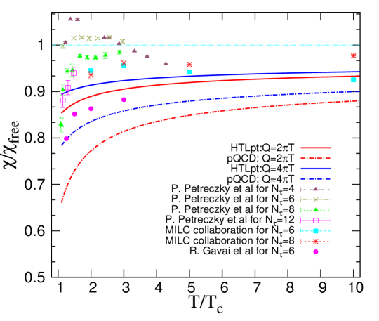
Figure 1: (Color online) The 2-flavour scaled QNS with that of free one as a function of $T/T_{C}$. The solid lines are for LO in HTLpt whereas the dashed lines are for LO (proportional to $g^{2}$) in pQCD blaizot ; toimela ; kapusta . The different choices of the renormalisation scale are $Q=2\pi T\ {\mbox{(red)}},\ \ {\mbox{and}}\ \ 4\pi T\ {\mbox{(blue)}}$. The symbols represent the various lattice data lat3 ; peter ; bazavov ; milc ; lat2 . The violet triangles (with $T_{c}=204\pm 2$ MeV), brown crosses (with $T_{c}196\pm 3$ MeV), green triangles (with $T_{c}=191\pm 2$ MeV) and purple squares (with $T_{c}=185\pm 5$ MeV) represent $p4$ lattice QCD data peter ; bazavov . The squares (cyan) and stars (saffron) are from asqtad lattice QCD data milc . The solid circles (purple) represent quenched QCD data lat2 for $T_{c}=0.49\Lambda_{\overline{MS}}$. The quark mass ranges between (0.1 to 0.2)$m_{s}$, where $m_{s}$ is the strange quark mass near its physical value. Note that further lowering the quark mass to its physical value seems to have a small effect qmass for $T>200$ MeV. The details of these lattice results are also summarised in Ref. peter1 .

Now we display in Fig. 1 the 2-flavour scaled QNS in LO with that of free gas as a function of temperature that shows significant improvement over pQCD results of order $g^{2}$  blaizot ; toimela ; kapusta . Moreover, it also shows the same trend as the available lattice results lat2 ; lat3 ; peter ; bazavov ; milc ; qmass ; peter1 , though there is a large variation among the various lattice results within the improved lattice (asqtad and p4) actions peter ; milc due to the higher order discretisation of the relevant operator associated with the thermodynamic derivatives. A detailed analysis on uncertainties of the ingredients in the lattice QCD calculations is presented in Refs. bazavov ; qmass . This calls for further investigation both on the analytic side by improving the HTL resummation schemes and on the lattice side by refining the various lattice ingredients.

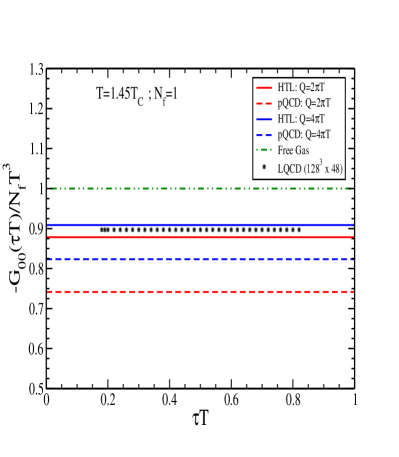
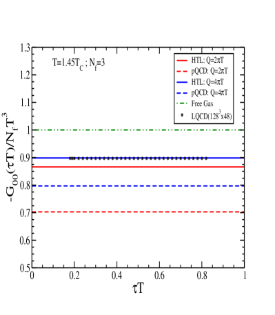
Figure 2: (Color online) The scaled temporal correlation function with $T^{3}$ for $N_{f}=1$ (left panel) and $N_{f}=3$ (right panel) at $T=1.45T_{C}$ for $Q=2\pi T$ (red) and $4\pi T$ (blue) as a function of scaled Euclidian time, $\tau T$. The symbols represent the recent lattice data karsch2 on lattices of size $128^{3}\times 48$ for quark mass $0.1T$ in quenched QCD.

Recently, an improved lattice calculation karsch2 has been performed within the quenched approximation of QCD where the temporal correlation function is determined to better than $1\%$ accuracy. Using the LO HTLpt QNS in (15) we now obtain the temporal correlation function in (14) and compare with the recent lattice data karsch2 . In Fig. 2 the scaled temporal correlation function with $T^{3}$ is shown for $N_{f}=1$ (left panel) and $N_{f}=3$ (right panel) at $T=1.45T_{c}$. We first note that the correlation functions both in HTLpt and pQCD have weak flavour dependence due to the temperature dependent coupling, $\alpha_{s}$ as discussed before. The LO HTLpt result indicates an improvement over that of the pQCD one blaizot ; toimela ; kapusta for different choices of the renormalisation scale as shown in Fig. 2. Also, the HTLpt result shows a good agreement to that of recent lattice gauge theory calculation karsch2 performed on lattices up to size $128^{3}\times 48$ in quenched approximation for a quark mass $\sim 0.1T$. We also note that unlike the dynamical spatial part of the correlation function in the vector channel the temporal part does not encounter any infrared problem in the low energy part as it is related to the static quantity through the thermodynamic sum rule associated with the corresponding symmetry, viz., the number conservation of the system. We also presented two extreme cases of HTLpt temporal correlation function at $T=1.2T_{C}$ in Fig. 3 and at $T\sim 3T_{C}$ in Fig. 4, respectively, for two different flavours and compare with the corresponding preliminary lattice data karsch3 , which are also found to be in good agreement. Finally, we also note that even if one compares improved lattice action (asqtad) data milc and recent quenched data karsch2 for QNS, the quantitative difference is within $5\%$ in the temperature domain $T_{C}\leq T\leq 3T_{C}$.

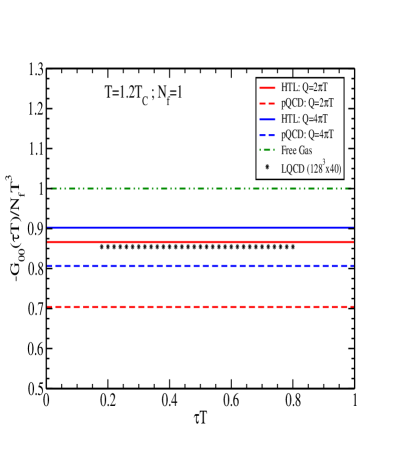
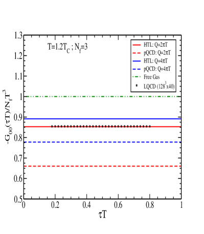
Figure 3: (Color online) Same as Fig. 2 but at $T=1.2T_{C}$ and the corresponding lattice data are preliminary karsch3 with lattice size $148^{3}\times 40$.

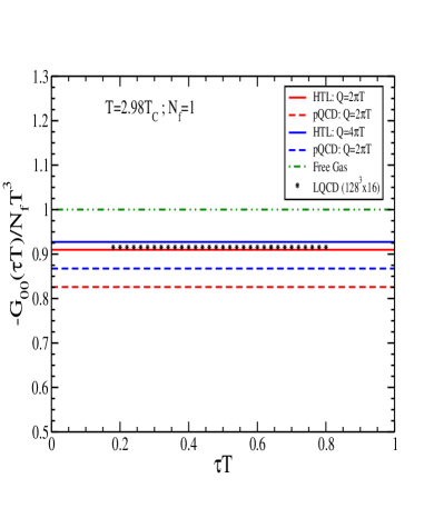
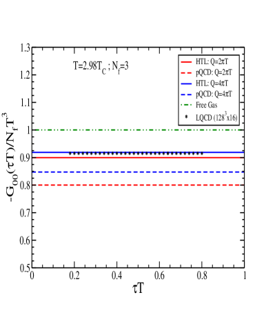
Figure 4: (Color online) Same as Fig. 2 but at $T=2.98T_{C}$ and the corresponding lattice data are preliminary karsch3 with lattice size $148^{3}\times 16$.

IV Conclusion

The LO QNS as a response of the conserved density fluctuation in HTLpt when compared with the available lattice data with improved lattice actions lat3 ; peter ; bazavov ; milc ; lat2 in the literature within their wide variation shows the same trend but deviates from those in certain extent. The same HTL QNS is used to compute the temporal part of the Euclidian correlation in the vector current which agrees quite well with that of improved lattice gauge theory calculations karsch2 ; karsch3 recently performed within the quenched approximation on lattices up to size $128^{3}\times 48$ for a quark mass $\sim 0.1T$. It is also interesting to note that the quantitative difference between the recent quenched approximation data karsch2 ; karsch3 and the full QCD data with improved (asqtad) lattice action milc for QNS is within $5\%$ in the temperature range $T_{c}\leq T\leq 3T_{c}$. Leaving aside the difference in ingredients in various lattice calculations, one can expect that the HTLpt and lattice calculations are in close proximity for quantities associated with the conserved density fluctuation.

- (1) T. Hashimoto, A. Nakamura, and I. O. Stamatescu, Nucl. Phys. B400, 267 (1993); G. Boyd, S. Gupta, F. Karsch, and E. Laermann, Z. Phys. C64, 331 (1991).
- (2) F. Karsch, M. G. Mustafa, and M. H. Thoma, Phys. Lett. B497, 249 (2001).
- (3) F. Karsch et al., Phys. Lett. B 530, 147 (2002).
- (4) W. M. Alberico, A. Beraudo, P. Czerski, and A Molinari, Nucl. Phys. A 775, 188 (2006); P. Czerski, Nucl. Phys. A 807, 11 (2008).
- (5) P. B. Arnold, G. D. Moore, and L. G. Yaffe, JHEP 0011, 001 (2000); JHEP 0112, 009 (2001); JHEP 0305, 051 (2003); P. Aurenche, F. Gelis, G. D. Moore, and H. Zaraket, JHEP 0212, 006 (2002).
- (6) NA49 Collaboration, M. Roland et al., Nucl. Phys. A638, 91c (1998); NA49 Collaboration, A. Appelshäser et al., Phys. Lett. B 459, 676 (1999); NA49 Collaboration, J. G. Reid et al., Nucl. Phys. A661, 407c (1999).
- (7) M. A. Stephanov, K. Rajagopal, and E. Shuryak, Phys. Rev. Lett. 81, 4816 (1998); Phys. Rev. D. 60, 114028 (1999); M. A. Stephanov, Phys. Rev. Lett. 102, 032301 (2009); M. Asakawa, U. Heinz, and B. Müller, Phys. Rev. Lett. 85, 2072 (2000); S. Jeon and V. Koch, Phys. Rev. Lett. 85, 2076 (2000).
- (8) D. Forster, Hydrodynamics Fluctuation, Broken Symmetry and Correlation Function (Benjamin/Cummings, Menlo Park, CA, 1975); H. B. Callen and T. A. Welton, Phys. Rev. 122, 34 (1961); R. Kubo, J. Phys. Soc. Jpn. 12, 570 (1957).
- (9) H.-T Ding, A. Francis, O. Kaczmarek, F. Karsch, E. Laermann, and W. Soeldner, Phys. Rev. D83, 034504 (2011).
- (10) N. Haque and M. G. Mustafa, arXiv:1007.2076[hep-ph].
- (11) E. Braaten and R. D. Pisarski, Nucl. Phys. B337, 569 (1990); Phys. Rev. Lett. 64, 1338 (1990).
- (12) P. Chakraborty, M. G. Mustafa, and M. H. Thoma, Eur. Phys. J. C. 23, 591 (2002); Phys. Rev. D 68, 085012 (2003).
- (13) J. O. Andersen, E. Braaten, E. Petitgirard, and M. Strickland, Phys. Rev. D66 (2002) 085016.
- (14) J. O. Andersen, M. Strickland, N. Su, Phys. Rev. Lett. 104, 122003 (2010); J. O. Andersen, M. Strickland, N. Su, JHEP 1008, 113 (2010); J. O. Andersen, L. E. Leganger, M. Strickland, N. Su, Phys. Lett. B696, 468 (2011); J. O. Andersen, L. E. Leganger, M. Strickland, N. Su, [arXiv:1103.2528 [hep-ph]].
- (15) B. Sheikholeslami and R. Wohlert, Nucl. Phys. B259, 572 (1985); M. Lüster et al., Nucl. Phys. B491, 344 (1997).
- (16) Y. Nakahara, M. Asakawa, and T. Hatsuda, Phys. Rev. D60, 091503 (1999); M. Asakawa, T. Hatsuda, and Y. Nakahara, Prog. Part. Nucl. Phys. 46, 459 (2001); I. Wetzorke, F. Karsch, in: C. P. Korthals-Altes (Ed.), Proceedings of the International Workshop on Strong and Electroweak Matter, World Scientific, 2001, p.193.
- (17) G. Aarts, C. Allton, J. Foley, S. Hands, and S. Kim, Phys. Rev. Lett. 99, 022002 (2007).
- (18) C. Greiner, N. Haque, M. G. Mustafa, and M. H. Thoma, Phys. Rev. C83, 014908 (2011), arXiv:1010.2169[hep-ph].
- (19) E. Braaten, R. D. Pisarski, and T. C. Yuan, Phys. Rev. Lett. 64, 2242 (1990).
- (20) M. H. Thoma, Nucl. Phys. (Proc. Suppl.) B92, 162 (2001); M. G. Mustafa and M. H. Thoma, Pramana 60, 711 (2003); A. Peshier and M. H. Thoma, Phys. Rev. Lett. 84, 841 (2000); M. G. Mustafa, A. Schäfer and M. H. Thoma, Phys. Rev. C61, 024902 (1999); Nucl. Phys. A 661, 653 (1999); P. Chakraborty, M. G. Mustafa, and M. H. Thoma, Phys. Rev. D 67, 114004 (2003).
- (21) S. M. H. Wong, Z. Phys. C53, 465 (1992).
- (22) T. Hatsuda and T. Kunihiro, Phys. Rep. 247, 221 (1994); T. Kunihiro, Phys. Lett. B 271, 395 (1991).
- (23) S. Gottlieb et al., Phys. Rev. Lett. 59, 2247 (1987); Phys. Rev. D 38, 2888 (1988); R. Gavai, J. Potvin, and S. Sanielevici, ibid. 40, R2743 (1989).
- (24) C. R. Allton et al., Phys. Rev. D 71, 054508 (2005).
- (25) P. Petreczky, P. Hegde, and A. Velytsky, PoS LAT2009:159, 2009, arXive:0911.0196 [hep-lat].
- (26) A. Bazavov et al., Phys. Rev. D80, 014504 (2009).
- (27) MILC Collaboration, C. Bernard et al., Phys. Rev. D71, 034504 (2005).
- (28) R. Gavai and S. Gupta, Phys. Rev. D 64, 074506 (2001); ibid. 65, 094515 (2002); R. Gavai, S. Gupta, and P. Majumdar, ibid. 65, 054506 (2002).
- (29) M. Cheng et al., Phys. Rev. D81, 054504 (2010).
- (30) P. Petreczky, Nucl. Phys. A830, 11c (2009).
- (31) L. McLerran, Phys. Rev. D 36, 3291 (1987); A. Vuorinen, ibid. 67, 074032 (2003); S. K. Ghosh, T. K. Mukherjee, and S. Raha, Mod. Phys. Lett. A21, 2067(2006).
- (32) Y. Hatta and T. Ikeda, Phys. Rev. D 67, 014028 (2003); C. Sasaki, B. Friman, and K. Redlich, ibid. 75, 054026 (2007); C. Ratti et al., Phys. Lett. B 649, 57 (2007).
- (33) S. K. Ghosh, T. K. Mukherjee, M. G. Mustafa, and R. Ray, Phys. Rev. D73, 114007 (2006); S. Mukherjee, M. G. Mustafa, and R. Ray, Phys. Rev. D75, 094015 (2007); S. K. Ghosh, T. K. Mukherjee, M. G. Mustafa, and R. Ray, Phys. Rev. D77, 094024 (2008); A. Bhattacharyya et al., Phys. Rev. D82, 014021 (2010); Phys. Rev. D 82, 114028 (2010); Phys. Rev. D 83, 014011 (2011).
- (34) K. Jo, Y. Kim, H. K. Lee, and S.-J. Sin, JHEP 0811, 040 (2008); Y. Kim et al., JHEP 1005, 038 (2010); K. Kim, Y. Kim, S. Takeuchi, and T. Tsukioka, [arXiv:1012.2667[hep-ph]].
- (35) B.-J. Schäfer and J. Wambach, Phys. Rev. D75, 085015 (2007); B.-J. Schäfer, M. Wagner, and J. Wambach, Phys. Rev. D81, 074013 (2010).
- (36) J.-P. Blaizot, E. Iancu, and A. Rebhan, Phys. Lett. B 523, 143 (2001); Eur. Phys. J. C 27, 433 (2003).
- (37) Y. Jiang, H.-x. Zhu, W.-m Sun, and H.-s. Zong, J. Phys. G 37, 055001 (2010).
- (38) E. Braaten and R. D. Pisarski, Phys. Rev. D 45, R1827 (1992).
- (39) J. I. Kapusta and C. Gale, Finite Temperature Field Theory Principle and Applications (Cambridge University Press, Cambridge, 1996), 2nd ed.
- (40) T. Toimela, Int. J. Theor. Phys. 24, 901 (1985).
- (41) J. O. Andersen, E. Braaten, and M. Strickland, Phys. Rev. Lett. 83, 2139 (1999); J. O. Andersen, E. Braaten, and M. Strickland, Phys. Rev. D 61, 014017 (1999); ibid. 61, 074016 (2000).
- (42) J. P. Blaizot, E. Iancu, and A. Rebhan, Phys. Rev. Lett. 83, 2906 (1999); Phys. Lett. B 470, 181 (1999); Phys. Rev. D 63, 065003 (2001).
- (43) F. Karsch, private communication.