Index Information Algorithm with Local Tuning for Solving Multidimensional Global Optimization Problems with Multiextremal Constraints

Abstract

Multidimensional optimization problems where the objective function and the constraints are multiextremal non-differentiable Lipschitz functions (with unknown Lipschitz constants) and the feasible region is a finite collection of robust nonconvex subregions are considered. Both the objective function and the constraints may be partially defined. To solve such problems an algorithm is proposed, that uses Peano space-filling curves and the index scheme to reduce the original problem to a Hölder one-dimensional one. Local tuning on the behaviour of the objective function and constraints is used during the work of the global optimization procedure in order to accelerate the search. The method neither uses penalty coefficients nor additional variables. Convergence conditions are established. Numerical experiments confirm the good performance of the technique.

Key Words:Global optimization, multiextremal constraints, local tuning, index approach.

1 Introduction

In the last decades there has been a growing interest in approaching Global Optimization problems by different numerical techniques (see, for example, [4]–[11], [15]–[20], [25, 27], [42]–[46] and references given therein). Such an interest is motivated by a large number of real-life applications where such problems arise (see, for example, [1]–[3], [6, 7, 8, 10, 15, 21, 22, 23, 25, 28, 30, 34, 36]). These problems often lead to deal with multiextremal non-differentiable objective function and constraints. In such a context the Lipschitz condition becomes the unique information about the problem.

It has been proved by Stephens and Baritompa [37] that if the only information about the objective function $\varphi(y)$ is that it belongs to the class of Lipschitz functions and the Lipschitz constant is unknown, there does not exist any deterministic or stochastic algorithm that, after a finite number of evaluations of $\varphi(y)$, is able to provide an underestimate of the global minimum $\varphi(y^{*})$. Of course, this result is very discouraging because usually in practice it is difficult to know the constant. Nevertheless, the necessity to solve practical problems remains. That is why in such problems instead of the statement (S1) ‘Find an algorithm able to stop in a given time and provide an $\varepsilon$-approximation of the global optimum $\varphi(y^{*})$’ the statement (S2) ‘Find an algorithm able to stop in a given time and return the lowest value of $\varphi(y)$ obtained by the algorithm’ is used. Under this statement, either the computed solution (possibly improved by a local analysis) is accepted by final users (engineers, physicists, chemists, etc.) or the global search is repeated with changed parameters of the algorithm.

Theoretical analysis of algorithms (depending on parameters) for solving problems (S2) is similar to analysis of penalty methods. It is proved for global optimization algorithms that for a fixed problem there exists a parameter $P^{*}$ such that parameters $P\geq P^{*}$ allow to solve the problem (obviously, the parameter $P^{*}$ is problem-dependent). The problem ‘How to determine $P^{*}$?’ is not discussed in such an analysis, and in every concrete case it is solved using additional information about the problem. For example, in methods using a given Lipschitz constant (see survey [12]) $P^{*}$ is the Lipschitz constant and it is not discussed how to obtain it. Other examples are diagonal methods (see [25]) and information algorithms (see [31, 38]) using similar parameters. For all those methods it is possible to prove that if a value $P\geq P^{*}$ is used as the parameter, then they converge only to global minimizers. An alternative approach is represented by methods converging to every point in the search domain (see [16, 44]).

In this paper a constrained Lipschitz global minimization problem is considered. In an informal way it can be stated as follows:

1. The objective function is multiextremal, non-differentiable, ’black box’, and requires a high time to be evaluated;

2. Constraints are non-convex (or even multiextremal) and non-differentiable, leading to a complex feasible region consisting of disjoint, non-convex sub-regions;

3. Both the objective function and constraints are Lipschitz functions with unknown Lipschitz constants;

4. Both the objective function and constraints may be partially defined, i.e., if a constraint is not satisfied at a point, the rest of constraints and the objective function may be not defined at that point.

It can be seen from this statement that the problem belongs to the class of problems considered in [37], thus statement (S2) will be used hereinafter. One promising way to face problem (i)–(iv) is the information approach introduced by Strongin in [38, 39, 40]. It uses Peano type space-filling curves (see [2, 5, 26, 38, 42] for examples of usage of space-filling curves in mathematical programming) to reduce the original Lipschitz multi-dimensional problem to a Hölder univariate one (a comprehensive presentation of this approach can be found in [42]). Global optimization of Hölder functions (see [9, 19, 45]) has given new tools for solving the reduced one-dimensional problem. Peano curves avoid constructions of support (or auxiliary) functions usually used in the multi-dimensional Lipschitz optimization (see, for example, [15, 17, 18, 25, 27, 42] and references given therein). Of course, if the user knows that the objective function is differentiable and/or the problem is convex, there is no sense to work with Peano curves and specific methods explicitly using information about differentiability or convexity can be applied. In contrast, when you deal with non-differentiable ’black box’ multiextremal problems, it is not possible to work with sophisticated techniques using derivatives (or other strong a priori suppositions) and such a reduction to one dimension can help significantly.

In this paper, a novel algorithm belonging to the family of information methods is proposed. It uses two powerful ideas for solving problem (i)–(iv). The first one is the index scheme (see [35, 38, 39, 41, 42]), allowing to solve Lipschitz problems where both the objective function $\varphi(y)$ and constraints $G_{i}(y),\,1\leq i\leq m,$ may be multiextremal and partially defined. Its importance increases in this case because it is not clear how to solve such problems by using, for example, the penalty approach. In fact, the latter requires that $\varphi(y)$ and $G_{i}(y),\,1\leq i\leq m,$ are defined over the whole search domain. It seems that missing values can be simply filled in with either a big number or the function value at the nearest feasible point. Unfortunately, in the context of Lipschitz algorithms, incorporating such ideas can lead to infinitely high Lipschitz constants, causing degeneration of the methods and non-applicability of the penalty approach. Thus, for problems where the Lipschitz condition is almost a unique additional information, the ability of the index scheme to work with partially defined problems becomes crucial. Moreover, the index scheme does not introduce any additional parameter and/or variable, whereas the penalty approach requiring determination of the penalty coefficient.

The second idea being at the basis of the new method is the local tuning on the behaviour of the objective function and constraints (see [31, 32, 34, 35]). Original information methods work with global adaptive estimates of the Lipschitz constants, i.e., the same estimates are used over the whole search region for $\varphi(y)$ and functions $G_{i}(y),\,1\leq i\leq m$. However, global estimates (adaptive or given a priori) of the Lipschitz constants may provide a poor information about the behavior of the objective function over every small sub-region of $D$. It has been shown in [25, 31, 32, 34, 35], for different classes of global optimization problems, that local estimates for different sub-regions of $D$ can accelerate the search significantly. Of course, it is necessary to balance global and local information about $\varphi(y)$ obtained by the method during the search. Such a balancing is very important because using only the local information can lead to missing the global solution (see [33, 37]).

The next section contains a formal statement of the problem (i)–(iv) and presents the new algorithm. Convergence conditions of the new method are established in Section 3. Numerical experiments collected in Section 4 show a satisfactory performance of the new algorithm in comparison with two global optimization techniques. Finally, Section 5 gives concluding remarks.

2 Theoretical background and the index information
algorithm with local tuning

We start by formulating the Lipschitz optimization problem satisfying requirements (i)–(iii). Find the constrained global minimum $\varphi^{*}$ and at least one minimizer $y^{*}$ such that

$$\varphi^{*}=\varphi(y^{*})=\min\{\varphi(y):y\in S,\quad G_{i}(y)\leq 0,\quad 1\leq i\leq m\},$$ (1)

where the search domain is the hyperinterval

$$S=\{y\in\mathbb{R}^{N}:a_{j}\leq y_{j}\leq b_{j},\quad 1\leq j\leq N\},$$

$\mathbb{R}^{N}$ is the $N$-dimensional Euclidean space, and the objective function $\varphi(y)$ (henceforth denoted as $G_{m+1}(y)$) and the functions $G_{i}(y),\,1\leq i\leq m$, of the constraints can be multiextremal and non-differentiable, satisfying the Lipschitz condition with unknown constants $0<\widehat{L}_{i}<\infty,\,1\leq i\leq m+1$, i.e.,

$$|G_{i}(y^{\prime})-G_{i}(y^{\prime\prime})|\leq\widehat{L}_{i}\,||y^{\prime}-y^{\prime\prime}||,\quad 1\leq i\leq m+1,\quad y^{\prime},y^{\prime\prime}\in S.$$ (2)

Without loss of generality, we shall consider the search domain $S=D$, where

$$D=\{y\in\mathbb{R}^{N}:-2^{-1}\leq y_{j}\leq 2^{-1},\quad 1\leq j\leq N\}.$$ (3)

Formulation (1)–(3) assumes that all the functions $G_{i}(y),\,1\leq i\leq m+1,$ can be evaluated in the whole region $D$. In order to incorporate requirement (iv), we shall assume that each function $G_{i}(y)$ is defined and computable only in the corresponding subset $Q_{i}\subset D$, where

$$Q_{1}=D,\quad Q_{i+1}=\{y\in Q_{i}:G_{i}(y)\leq 0\},\quad 1\leq i\leq m.$$ (4)

The above assumption also imposes the order in which the functions $G_{i}(y),1\leq i\leq m$, are evaluated. In many applications this order is determined by the nature of the problem. In other cases the user introduces a specific order suit for some reasons (for example, first verify easier computable constraints). In view of (4), the initial problem (1)–(3) is rewritten as

$$\varphi(y^{*})=\min\{G_{m+1}(y):y\in Q_{m+1}\},$$ (5)

$$|G_{i}(y^{\prime})-G_{i}(y^{\prime\prime})|\leq L_{i}\,||y^{\prime}-y^{\prime\prime}||,\quad y^{\prime},y^{\prime\prime}\in Q_{i},\quad 1\leq i\leq m+1,$$ (6)

where $L_{i}\leq\widehat{L}_{i}$.

In order to start the description of the method it is necessary to remind the idea of the space-filling curves. Such curves were first introduced by Peano in [24] and Hilbert in [13] and are fractal objects constructed on the principle of self-similarity. They possess the property ‘to fill’ any cube $D$ in $\mathbb{R}^{N}$, i.e., they pass through every point of $D$. An example of construction of such a curve (see  [29, 42] for details) is given in Fig. 1. Naturally, in numerical algorithms, approximations of the curve are used (Fig. 1 presents approximations of levels one to four).

Figure 1: Approximations of levels one to four to the Peano (Hilbert) curve in two dimensions.

It has been shown in [5, 38, 40] (see also [42]) that the multi-dimensional problem

$$\varphi^{*}=\varphi(y^{*})=\min\{\varphi(y):\;y\in D\},$$ (7)

where $\varphi(y)$ is a Lipschitz function with constant $L$, $0<L<\infty,$ can be reduced by a Peano-type space-filling curve $y(x)$ to the one-dimensional problem

$$f^{*}=f(x^{*})=\min\{f(x),\;x\in[0,1]\},$$ (8)

where the notation $f(x)=\varphi(y(x))$ is used for the obtained reduced one-dimensional function. Moreover, (see Theorem 8.1 in [42]), the function $f(x)$ satisfies the Hölder condition

$$|f(x^{\prime})-f(x^{\prime\prime})|\leq H\,|x^{\prime}-x^{\prime\prime}|^{1/N},\,\quad x^{\prime},x^{\prime\prime}\in[0,1],$$ (9)

in the Hölder metric

$$\rho(x^{\prime},x^{\prime\prime})=|x^{\prime}-x^{\prime\prime}|^{1/N},$$ (10)

where $N$ is from (3) and $H=2\,L\,\sqrt{N+3}$.

By applying the same curve $y(x)$ to the functions $G_{i}(y),\;1\leq i\leq m+1$, and using designations $g_{i}(x)=G_{i}(y(x))$, the multi-dimensional problem (5)–(6) is reduced to the following constrained one-dimensional problem (11)–(13):

$$g_{m+1}^{*}=g_{m+1}(x^{*})=\min\{g_{m+1}(x):x\in q_{m+1}\},$$ (11)

where the region $q_{m+1}$ is defined by the relations

$$q_{1}=[0,1],\quad q_{i+1}=\{x\in q_{i}:g_{i}(x)\leq 0\},\quad 1\leq i\leq m.$$ (12)

and the reduced functions $g_{i}(x),1\leq i\leq m+1$, satisfy the corresponding Hölder conditions

$$|g_{i}(x^{\prime})-g_{i}(x^{\prime\prime})|\leq H_{i}\,|x^{\prime}-x^{\prime\prime}|^{1/N},\quad x^{\prime},x^{\prime\prime}\in q_{i},\quad 1\leq i\leq m+1,$$ (13)

with the constants $H_{i}=2\,L_{i}\,\sqrt{N+3}$, where $L_{i},1\leq i\leq m+1$, are from (6). Note that for the regions $Q_{i}$ from (4) and $q_{i}$ from (12) the following relation holds:

$$Q_{i}=\{y(x):x\in q_{i}\},\quad 1\leq i\leq m+1.$$

This problem may be rewritten by using the index scheme proposed in [39, 41] (see also [40]). The scheme is an alternative to traditional penalty methods. Instead of combining the objective and constraint functions into a penalty one (and the need to define in a proper way penalty coefficients), the scheme does not introduce any additional parameter or variable and evaluates constraints one at a time at every point where it has been decided to try to evaluate $g_{m+1}(x)$. The function $g_{i}(x)$ is calculated only if all inequalities

$$g_{j}(x)\leq 0,\quad 1\leq j<i,$$

have been satisfied. In its turn, the objective function $g_{m+1}(x)$ is evaluated only for those points where all the constraints have been satisfied.

The index scheme juxtaposes to every point of the interval $[0,1]$ an index

$$\nu=\nu(x),\quad 1\leq\nu\leq m+1,$$

which is defined by the conditions

$$g_{j}(x)\leq 0,\quad 1\leq j\leq\nu-1,\quad g_{\nu}(x)>0,$$ (14)

where for $\nu=m+1$ the last inequality is omitted. Thus, $\nu(x)$ represents the number of the first constraint not satisfied at $x$ when $\nu(x)<m+1$. Then $\nu(x)=m+1$ means that all constraints were satisfied at $x$ and the objective function $g_{m+1}(x)$ may be evaluated at this point.

Let us now define an auxiliary function $\Phi(x)$ as follows

$$\Phi(x)=g_{\nu}(x)-\left\{\begin{array}[]{ll}0,&\nu(x)<m+1,\\[5.0pt] g^{*}_{m+1},&\nu(x)=m+1,\end{array}\right.$$ (15)

where $g^{*}_{m+1}$ is the solution of the problem (11)–(13). Due to (14) and (15), the function $\Phi(x)$ has the following properties:

• $\Phi(x)>0$, when $\nu(x)<m+1$;

• $\Phi(x)\geq 0$, when $\nu(x)=m+1$;

• $\Phi(x)=0$, when $\nu(x)=m+1$ and $g_{m+1}(x)=g^{*}_{m+1}$;

• $\Phi(x)$ is not continuous at the a priori unknown boundary points of the sets $q_{i},2\leq i\leq m+1$.

Thus, the global minimizer of the constrained problem (11)–(13) coincides with the solution $x^{*}$ of the following unconstrained problem

$$\Phi(x^{*})=\min\{\Phi(x):x\in[0,1]\}.$$ (16)

Of course, instead of the fractal Peano curve $y(x)$ its $d$-level approximation $y_{d}(x)$ is used for evaluation of $\Phi(x)$ (approximations of levels one to four are shown in Fig. 1, from where it can be seen how a $d$-level approximation is obtained).

The new index information global optimization algorithm with local tuning presented below generalizes and evolves two methods. On the one hand, the information global optimization algorithm with local tuning proposed in [31] for solving the problem (7) and, consequently, the problem (8)–(9). On the other hand, the index algorithm with local tuning proposed in [35] for solving the one-dimensional problem

$$\min\{f(x):x\in[a,b],\;g_{i}(x)\leq 0,\;1\leq i\leq m\}$$

where both $f(x)$ and $g_{i}(x),1\leq i\leq m,$ are Lipschitz continuous functions.

During every iteration of the algorithm a point $x\in[0,1]$ is chosen and the value $\Phi(x)$ is evaluated (hereinafter such an evaluation will be called a trial and the corresponding point $x$ a trial point). Suppose now that $k$ iterations of the algorithm have already been executed (two initial trials are done at the end points $x^{0}=0$ and $x^{1}=1$). The point $x^{k+1},k\geq 1$, is determined by the following algorithm.

Step 1.

The points $x^{0},\ldots,x^{k}$ of the previous iterations are renumbered by subscripts as follows

$$0=x_{0}<x_{1}<\cdots<x_{i}<\cdots<x_{k}=1.$$

Step 2.

To each point $x_{i}$ associate the index $\nu_{i}=\nu(x_{i})$, and the value

$$z_{i}=g_{\nu_{i}}(x_{i})-\left\{\begin{array}[]{ll}0,&\nu_{i}<m+1,\\[5.0pt] z_{k}^{*},&\nu_{i}=m+1,\par\end{array}\right.$$

where

$$z_{k}^{*}=\min\{g_{m+1}(x_{i}):0\leq i\leq k,\nu(x_{i})=m+1\}.$$ (17)

The value $z_{k}^{*}$ estimates the unknown value $g^{*}_{m+1}$ from (15) on the basis of the available data.

Step 3.

Calculate lower bounds $\mu_{j}$ for the global Hölder constants $H_{j}$ of the functions $g_{j}(x),1\leq j\leq m+1,$ as follows

$$\mu_{j}=\max\Big{\{}\frac{|z_{p}-z_{q}|}{(x_{p}-x_{q})^{1/N}}:0\leq q<p\leq k,\nu_{p}=\nu_{q}=j\Big{\}}.$$ (18)

Whenever $\mu_{j}$ can not be calculated, set $\mu_{j}=0$.

Step 4.

For each interval $[x_{i-1},x_{i}],i=1,\ldots,k$, calculate the values

$$M_{i}=\max\{\lambda_{i},\gamma_{i},\xi\}$$ (19)

that estimate the local Hölder constant over the interval $[x_{i-1},x_{i}]$. The values $\lambda_{i}$ and $\gamma_{i}$ reflect the influence on $M_{i}$ of the local and global information obtained during the previous $k$ iterations, $\xi$ is a small number - parameter of the method. The values $\lambda_{i}$ and $\gamma_{i}$ are defined by

$$\lambda_{i}=\max\{l_{i},c_{i},r_{i}\},$$ (20)

where

$$\begin{array}[]{ll}c_{i}&=\left\{\!\!\!\begin{array}[]{cl}\displaystyle{\frac{|z_{i}-z_{i-1}|}{(x_{i}-x_{i-1})^{1/N}}},&\mbox{if}\;\nu_{i}=\nu_{i-1}\\[15.0pt] 0,&$ otherwise$\end{array}\right.\\[25.0pt] l_{i}&=\left\{\!\!\!\begin{array}[]{cl}\displaystyle{\frac{|z_{i-1}-z_{i-2}|}{(x_{i-1}-x_{i-2})^{1/N}}},&\mbox{if}\;i\geq 2,\quad\nu_{i-2}=\nu_{i-1},\nu_{i-1}\geq\nu_{i}\\[15.0pt] 0,&\mbox{otherwise}\end{array}\right.\\[25.0pt] r_{i}&=\left\{\!\!\!\begin{array}[]{cl}\displaystyle{\frac{|z_{i+1}-z_{i}|}{(x_{i+1}-x_{i})^{1/N}}},&\mbox{if}\;i\leq k-1,\quad\nu_{i+1}=\nu_{i},\nu_{i}\geq\nu_{i-1}\\[15.0pt] 0,&$ otherwise$\end{array}\right.\end{array}$$

and

$$\gamma_{i}=\frac{\mu_{j}(x_{i}-x_{i-1})^{1/N}}{X^{\rm max}_{j}},\hskip 17.07164ptj=\max\{\nu_{i},\nu_{i-1}\},$$ (21)

where $X^{\rm max}_{j}=\!\max\{(x_{i}-x_{i-1})^{1/N}:\;\max\{\nu_{i},\nu_{i-1}\}=j,\quad 1\leq i\leq k\}$.

Step 5.

For each interval $[x_{i-1},x_{i}],i=1,\ldots,k$, calculate the characteristic of the interval

$$R_{i}=\left\{\begin{array}[]{ll}\Delta_{i}+\,\displaystyle{\frac{(z_{i}-z_{i-1})^{2}}{(rM_{i})^{2}\Delta_{i}}-\,\frac{2\,(z_{i}+z_{i-1})}{rM_{i}}},&\nu_{i}=\nu_{i-1}\\[10.0pt] 2\,\Delta_{i}-\,\displaystyle{\frac{4\,z_{i}}{rM_{i}}},&\nu_{i}>\nu_{i-1}\\[10.0pt] 2\,\Delta_{i}-\,\displaystyle{\frac{4\,z_{i-1}}{rM_{i}}},&\nu_{i-1}>\nu_{i}\end{array}\right.$$ (22)

where $\Delta_{i}=(x_{i}-x_{i-1})^{1/N}$ and $r>1$ is a real value – the reliability parameter of the method.

Step 6.

Choose the interval $[x_{t-1},x_{t}]$ having the maximal characteristic as follows

$$t=\min\{\arg\max\{R_{i}:1\leq i\leq k\}\}.$$ (23)

Step 7.

If the interval $[x_{t-1},x_{t}]$ is such that

$$(x_{t}-x_{t-1})^{1/N}>\delta,$$

where $\delta$ is a given tolerance, go to Step 8. Otherwise Stop.

Step 8.

Execute the $(k+1)$-th iteration at the point

$$x^{k+1}\!=\frac{x_{t}+x_{t-1}}{2}-\frac{{\rm sign}(z_{t}-z_{t-1})|z_{t}-z_{t-1}|^{N}}{2\,r\,M_{t}^{N}},$$ (24)

if $\nu_{t}=\nu_{t-1}$. In all other cases do it at the point

$$x^{k+1}\!=(x_{t}+x_{t-1})/2.$$ (25)

Set $k=k+1$ and go to Step 1.

If trial points with the index $m+1$ have been generated by the algorithm then the value $z_{k}^{*}$ from (17) can be taken as an estimate of the global minimum $\varphi^{*}$ from (1) and the corresponding point $y_{d}(x_{k}^{*})$ such that $z_{k}^{*}=g_{m+1}(x_{k}^{*})$ as an estimate of the point $y^{*}$. If no points with the index $m+1$ have been generated by the algorithm then it is necessary to continue the search with changed parameters of the method.

Let us give a few remarks on the algorithm introduced above. The information algorithms are derived as optimal statistical decision functions within the framework of a stochastic model representing the function to be optimized as a sample of a random function. The characteristic $R_{i}$ in terms of the information approach (see [38, 42]) may be interpreted (after normalization) as the probability of finding a global minimizer within the interval $[x_{i-1},x_{i}]$ based on the data available during the current iteration. The method uses in its work four parameters: $d,r,\xi,$ and $\delta$. Their choice will be discussed in Section 4 while presenting the numerical experiments.

For every sub-interval $[x_{i-1},x_{i}],1\leq i\leq k$, global estimates $\mu_{j}$ of the global Hölder constants $H_{j},1\leq j\leq m+1$, from (13) are not used. In contrast, local estimates $M_{i},1\leq i\leq k$, from (19) are adaptively determined. The values $\lambda_{i}$ and $\gamma_{i}$ reflect the influence on $M_{i}$ of the local and global information obtained during the previous $k$ iterations. When the interval $[x_{i-1},x_{i}]$ is small, then $\gamma_{i}$ is small too (see (21)) and, due to (19), the local information represented by $\lambda_{i}$ has major importance. The value $\lambda_{i}$ is calculated by considering the intervals $[x_{i-2},x_{i-1}],\;[x_{i-1},x_{i}],$ and $[x_{i},x_{i+1}]$ (see (20)) as those which have the strongest influence on the local estimate. When the interval $[x_{i-1},x_{i}]$ is very wide, the local information is not reliable and the global information represented by $\gamma_{i}$ is used. Thus, local and global information are balanced in the values $M_{i},1\leq i\leq k$. Note that the method uses the local information over the whole search region $[0,1]$ (and, consequently, over the whole multi-dimensional domain $D$) during the global search both for the objective function and constraints (being present in a implicit form in the auxiliary function $\Phi(x)$).

3 Convergence conditions

In the further theoretical consideration it is assumed that each region $Q_{i},2\leq i\leq m+1,$ from (4) is a union of $T_{i}$ disjoint sub-regions $Q_{i}^{j},\;1\leq j\leq T_{i},$ having positive volume (in general, the numbers $T_{i}$ are unknown to the user) where each sub-region $Q_{i}^{j},1\leq j\leq T_{i},2\leq i\leq m+1,$ is robust and can be non-convex. It is assumed that the feasible region $Q_{m+1}$ is nonempty. Recall that a set $B$ is robust if for each point $\beta$ belonging to the boundary of $B$ and for any $\varepsilon>0$ there exists an $\varepsilon$-neighborhood $\varepsilon(\beta)$ such that $\varepsilon(\beta)\bigcap B$ has a positive volume. Supposition about robustness of the sets $Q_{i}^{j}$ is quite natural in engineering applications (for example, in optimal control) where the optimal solution must have an admissible neighborhood of positive volume. This requirement is a consequence of the inevitable inaccuracy of the physical systems, and ensures that small changes of the parameters of the system will not lead the solution to leave the feasible region.

Theoretical results presented in this section have the spirit of existence theorems. They show (similarly to the penalty approach) that for a given problem there exist parameters of the method allowing to solve this fixed problem. Recall that (see [37]) the information available from the statement (5)–(6) is not sufficient for establishing concrete values of the parameters. These should be chosen from an additional information about the nature of the practical problem under consideration (see the next section).

The first result links solutions of the original multi-dimensional problem (5)–(6) to the solutions of the corresponding one-dimensional problem (11)–(13) reduced via the curve $y_{d}(x)$. It shows that for any given $\varepsilon>0$ there exists a level $d$ such that the approximation $y_{d}(x)$ passes through the $\varepsilon$-neighborhood of the global solution $y^{*}$ of the problem (5)–(6). Moreover, the global solution $y_{d}^{*}$ of the reduced problem (11)–(13) will also belong to the same $\varepsilon$-neighborhood.

Theorem 1

For every problem (5)–(6) having the unique solution $y^{*}$, and a given accuracy $\varepsilon>0$, there exists a subdivision level $d$ such that in the $\varepsilon$-neighborhood $\varepsilon(y^{*})$ of the global minimizer $y^{*}$ there exists a segment $h$ of the level-$d$ approximating curve $y_{d}(x)$ with the following properties:

1. the segment $h$ belongs to $Q_{m+1}\cap\varepsilon(y^{*})$ and has a finite positive length;

2. the segment $h$ contains the global minimizer $y_{d}^{*}$ of the problem

   $$\varphi(y_{d}^{*})=\min\{G_{m+1}(y_{d}(x)):\;y_{d}(x)\in Q_{m+1},x\in[0,1]\}.$$ (26)

Proof. We have assumed that the feasible region $Q_{m+1}$ is the union of $T_{m+1}$ robust subregions $Q_{m+1}^{j},\;1\leq j\leq T_{m+1}$. Suppose that $y^{*}\in Q_{m+1}^{p}$, where $Q_{m+1}^{p}$ is one of those subregions. Then $Q_{m+1}^{p}\cap\varepsilon(y^{*})$ is a robust set with a nonzero volume. This means that by increasing the accuracy of approximation it is possible to find an approximation level $d$ such that the curve $y_{d}(x)$ will have a segment $h\subset Q_{m+1}^{p}\cap\varepsilon(y^{*})$ with the required properties.

An illustration to Theorem 1 is given in Fig. 2, where a region $Q_{m+1}^{p}$ is shown in grey color. Analogously, if problem (5)–(6) has more than one solution, an approximation level $d$ providing existence of such intervals having finite positive lengths can be found for each of global minimizers. Of course, (26) may be satisfied only for one interval but, anyway, all these intervals will contain $\varepsilon$-approximations of the global solution. Thus, Theorem 1 allows us to concentrate the further theoretical investigation on the behaviour of the method during the solution of problem (16).

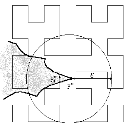
Figure 2: Illustration of existence of a subdivision level $d$ allowing an $\varepsilon$-approximation $y_{d}^{*}$ of the global solution $y^{*}$ such that the point $y_{d}^{*}$ is the global minimizer of the objective function $G_{m+1}(y_{d}(x))$ on $Q_{m+1}\cap y_{d}(x)$.

Lemma 1

Let $\bar{x}$ be a limit point of the infinite sequence $\{x^{k}\}$ generated by the algorithm and let $i=i(k)$ be the number of an interval $[x_{i-1},x_{i}]$ containing this point during the $k$-th iteration. Then

$$\lim_{k\rightarrow\infty}(x_{i(k)}-x_{i(k)-1})^{1/N}=0,$$ (27)

and for every $\sigma>0$ there exists an iteration number $n(\sigma)$, such that the inequality

$$R_{i(k)}<\sigma$$ (28)

holds for all $k\geq n(\sigma)$.

Proof. The new trial point $x^{k+1}$ from (24) or (25) falls into an interval $[x_{i-1},x_{i}]$ (where $i(k)=t(k)$ is determined by (23)), and divides this one into two sub-intervals

$$[x_{i-1},x^{k+1}],\quad[x^{k+1},x_{i}].$$

Let us show that there exists a number $\alpha$, independent of the iteration number $k$, such that

$$\max\{x_{i}-x^{k+1},x^{k+1}-x_{i-1}\}\leq\alpha(x_{i}-x_{i-1}),\quad 0.5\leq\alpha<1,$$ (29)

holds for these intervals. In the case $\nu_{t}\neq\nu_{t-1}$ the estimate (29) is obtained immediately from (25) by taking $\alpha_{1}=0.5$. In the opposite case, from (19)–(21) it follows that

$$\frac{\mid z_{t}-z_{t-1}\mid^{N}}{M_{t}^{N}}\leq x_{t}-x_{t-1},\quad\nu_{t}=\nu_{t-1}.$$ (30)

From this inequality, (24), and the fact that $r>1$ we can conclude that in the case $\nu_{t}=\nu_{t-1}$ (29) is true for $\alpha_{2}=(r+1)/(2r)$. Since $\alpha_{2}>\alpha_{1}$, (29) is proved by taking $\alpha=\alpha_{2}$.

Now, considering (29) together with the existence of a sequence converging to $\bar{x}$ (this point is a limit point of $\{x^{k}\}$), we can deduce that (27) holds. Note that in the case when two intervals containing the point $\bar{x}$ there exist (i.e., when $\bar{x}\in\{x^{k}\}$) the number $i=i(k)$ is juxtaposed to the interval for which (27) takes place.

Let us prove (28). From (22) and (30) we obtain, for intervals with indexes $\nu_{i}=\nu_{i-1}$,

$$R_{i}\leq(1+r^{-2})(x_{i}-x_{i-1})^{1/N}\leq 2(x_{i}-x_{i-1})^{1/N},$$

taking into account that $\Phi(x)\geq 0$ and $r>1$. The last estimate holds also for intervals with $\nu_{i}\neq\nu_{i-1}$. This inequality and (27) lead to (28).

Theorem 2

Let $x^{*}$ be any solution to the problem (16) and $j=j(k)$ be the number of an interval $[x_{j-1},x_{j}]$ containing this point during the $k$-th iteration. Then, if for $k\geq k^{*}$ the condition

$$rM_{j}>\left\{\begin{array}[]{ll}2^{1-1/N}C_{j}+\sqrt{2^{2-2/N}C_{j}^{2}-D_{j}^{2}},&\nu_{j-1}=\nu_{j},\\ 2C_{j},&\nu_{j-1}\neq\nu_{j},\end{array}\right.$$ (31)

holds, the point $x^{*}$ will be a limit point of $\{x^{k}\}$. The values $C_{j}$ and $D_{j}$ used in (31) are

$$C_{j}=\left\{\begin{array}[]{ll}z_{j-1}/(x^{*}-x_{j-1})^{1/N},&\nu_{j-1}>\nu_{j},\\ \max\{z_{j-1}/(x^{*}-x_{j-1})^{1/N},z_{j}/(x_{j}-x^{*})^{1/N}\},&\nu_{j-1}=\nu_{j},\\ z_{j}/(x_{j}-x^{*})^{1/N},&\nu_{j-1}<\nu_{j},\end{array}\right.$$ (32)

$$D_{j}=\left\{\begin{array}[]{ll}\mid z_{j}-z_{j-1}\mid/(x_{j}-x_{j-1})^{1/N},&\nu_{j-1}=\nu_{j},\\ 0,&\mbox{\rm otherwise}.\end{array}\right.$$ (33)

Proof. Consider the case $\nu_{j-1}=\nu_{j}$. Due to (32), we can write

$$z_{j-1}\leq C_{j}(x^{*}-x_{j-1})^{1/N},$$ (34)

$$z_{j}\leq C_{j}(x_{j}-x^{*})^{1/N}.$$ (35)

Now, by using (34), (35), and the designation

$$\beta=(x^{*}-x_{j-1})/(x_{j}-x_{j-1}),$$

we deduce

$$\begin{array}[]{ll}z_{j-1}+z_{j}&\leq C_{j}((x^{*}-x_{j-1})^{1/N}+(x_{j}-x^{*})^{1/N})\\ &=C_{j}(\beta^{1/N}+(1-\beta)^{1/N})(x_{j}-x_{j-1})^{1/N}\\ &\leq C_{j}(x_{j}-x_{j-1})^{1/N}\max\{\beta^{1/N}+(1-\beta)^{1/N}:0\leq\beta\leq 1\}\\ &=2^{1-1/N}C_{j}(x_{j}-x_{j-1})^{1/N}.\end{array}$$

By using this estimate and (31), (33), we obtain

$$\begin{array}[]{ll}R_{j(k)}&=(x_{j}-x_{j-1})^{1/N}+\displaystyle{\frac{(z_{j-1}\!-\!z_{j})^{2}}{(rM_{j})^{2}(x_{j}\!-\!x_{j-1})^{1/N}}-\frac{2(z_{j-1}\!+\!z_{j})}{rM_{j}}}\\ \\ &\geq(x_{j}\!-\!x_{j-1})^{1/N}(1\!+\!D^{2}_{j}(rM_{j})^{-2}\!-\!2^{2-1/N}C_{j}(rM_{j})^{-1}).\end{array}$$

Now, due to (31), we can conclude that

$$R_{j(k)}>0.$$ (36)

In the case $\nu_{j-1}>\nu_{j}$ the estimate (34) takes place due to (32). From (22) it follows that

$$R_{j(k)}\geq 2(x_{j}-x_{j-1})^{1/N}(1-2C_{j}(rM_{j})^{-1}),$$

and, consequently, by taking into consideration (31), the inequality (36) holds in this case also. Truth of (36) for $\nu_{j-1}<\nu_{j}$ is demonstrated by analogy.

Assume now that $x^{*}$ is not a limit point of the sequence $\{x^{k}\}$. Then, there exists a number $K_{s}$ such that for all $k\geq K_{s}$ the interval $[x_{j-1},x_{j}]$, $j=j(k)$, is not changed, i.e., new points will not fall into this interval.

Consider again the interval $[x_{i-1},x_{i}]$ from Lemma 1 containing a limit point $\bar{x}$. It follows from (28) that there exists a number $K_{p}$ such that

$$R_{i(k)}<R_{j(k)}$$

for all $k\geq k^{*}=\max\{K_{s},K_{p}\}$. This means that, starting from the iteration $k^{*}$, the characteristic of the interval $[x_{i-1},x_{i}],i=i(k),k\geq k^{*}$, is not maximal. Thus, a trial will fall into the interval $[x_{j-1},x_{j}]$. But this fact contradicts our assumption that $x^{*}$ is not a limit point.

Corollary 1

Given the conditions of Theorem 2, Theorem 1 ensures that trial points generated by the algorithm will fall in the feasible sub-region $Q_{m+1}\cap\varepsilon(y^{*})$.

Theorems 1, 2 generalize for the constrained case (11)–(13) results established in [31] for the Lipschitz global optimization problems with box constraints. Usually, Lipschitz global optimization algorithms need an overestimate (adaptive or a priori given) of the global Lipschitz constant for the whole search region (see, for example, survey [12] and references given therein). The new algorithm does not need knowledge of the precise Lipschitz constants for the functions $G_{i}(y),\,1\leq i\leq m+1,$ over the whole search region. In fact, the point $y^{*}$ (as all points in $D$) has up to $2^{N}$ images on the Peano curve. To obtain an $\varepsilon$-approximation of $y^{*}$ it is sufficient the fulfillment of the condition (31) (which is significantly weaker than the Lipschitz condition) for only one image of $y^{*}$ on a segment $h$ of the curve such that $h\subset Q_{m+1}\cap\varepsilon(y^{*})$. In the rest of the region $D$ the constants $L_{i},\,1\leq i\leq m+1,$ can be underestimated.

In the preceding it has been established that, if condition (31) is satisfied, the trial sequence $\{x^{k}\}$ generated by the algorithm converges to the global minimizer $x^{*}$ of the function $\Phi(y)$ and, consequently, the corresponding sequence $\{y_{d}(x^{k})\}$ converges to the global minimizer $y^{*}$ of the function $\varphi(y)$. In the following theorem it is proved that for any problem (5)–(6) there exists a continuum of values of $r$ satisfying (31).

Theorem 3

For any problem (5)–(6) a value $r^{*}$ exists such that, for all $r>r^{*}$, condition (31) is satisfied for all iteration numbers $k\geq 1$.

Proof. Let us choose

$$r^{*}=2^{3-1/N}\xi^{-1}\sqrt{N+3}\;\max\{L_{i}:\;1\leq i\leq m+1\},$$ (37)

and take a value $r>r^{*}$. Since, due to (13),

$$H_{i}=2\,\sqrt{N+3}\;L_{i},\quad 1\leq i\leq m+1,$$

the value $r^{*}$ from (37) can be rewritten as

$$\begin{array}[]{ll}r^{*}&=2^{2-1/N}\xi^{-1}H,\\[5.0pt] H&=\max\{H_{i}:1\leq i\leq m+1\}.\end{array}$$

For all $k\geq 1$, for the estimates $M_{j(k)}$ and the values $C_{j(k)}$ from (32) the inequalities

$$\xi\leq M_{j(k)},\hskip 14.22636ptC_{j(k)}\leq H,$$

hold. Then, when the interval $[x_{j-1},x_{j}]$ has $\nu_{j}=\nu_{j-1}$, it follows from (37) that

$$\begin{array}[]{lll}rM_{j(k)}&>r^{*}M_{j(k)}&\geq r^{*}\xi=2^{2-1/N}H\\[5.0pt] &>2^{2-1/N}C_{j}&\geq 2^{1-1/N}C_{j}+\sqrt{2^{2-2/N}C_{j}^{2}-D_{j}^{2}}.\end{array}$$

To complete the proof it is sufficient to note that in the case $\nu_{j}\neq\nu_{j-1}$ the last estimate can be substituted by

$$2^{2-1/N}C_{j}>2\,C_{j},$$

because $N\geq 2$. Thus, for the chosen $r>r^{*}$, condition (31) is satisfied.

Theorem 2 establishes sufficient convergence conditions for the method. Theorem 3 ensures that there exists a continuum of values of the parameter $r$ satisfying these conditions. However, these theorems just prove existence of such values and can not be considered as an instrument for determining the value $r^{*}$. This value is problem-dependent and can not be found without additional information about the objective function and constraints. In presence of such information it is possible to solve the problem (S1), otherwise only the problem (S2) can be faced.

Condition (31) gives us a suggestion how to choose a reasonable value of $r$ to start optimization in the case (S2). Note that the value $D_{j}$ from (34) can be equal to zero. The role of $M_{j}$ is to estimate $C_{j}$. Thus, if $D_{j}=0$ and $M_{j}=C_{j}$, it follows from (31) that $r$ should be greater than $2^{2-1/N}$. Some practical advises for the choice of the method parameters will be given in the next section.

4 Numerical experiments

This section presents numerical experiments that investigate the performance of the proposed algorithm in solving some test problems. The first three problems are taken from the literature; the other problems are proposed by the authors. All the methods have been implemented in MATLAB [43] and the experiments have been executed at a PC with Pentium III $733$MHz processor.

Experiment 1. In the first experiment the new algorithm is compared with two methods: (i) the information algorithm for solving problems with box constraints proposed in [39], combined with the penalty approach; (ii) the original index information algorithm proposed by Strongin and Markin in [39]–[41], that does not use the local tuning. These methods have been chosen for comparison because all of them have similar computational cost for a single iteration (of course, if the cost required for the search of the penalty coefficient allowing to solve the problem is not taken in consideration for the method (i)), they use Peano curves, and have the same stopping rule. Since the penalty approach needs the objective function and constraints defined over the whole search region, test problems enjoying this property have been chosen.

Problem 1. The first problem (see [41]) is to minimize the function

$$\begin{array}[]{ll}\varphi(y)=&-1.5\,y_{1}^{2}\exp(1-y_{1}^{2}-20.25\,(y_{1}-y_{2})^{2})\\[3.0pt] &-\,(0.5\,(y_{1}-1)(y_{2}-1))^{4}\exp(2-(0.5\,(y_{1}-1))^{4}-(y_{2}-1)^{4})\end{array}$$ (38)

over the rectangle $D=[0,4]\times[-1,3]$, under the constraints

$$\begin{array}[]{l}G_{1}(y)=0.01\,((y_{1}-2.2)^{2}+(y_{2}-1.2)^{2}-2.25)\leq 0,\\[3.0pt] G_{2}(y)=100\,(1-(y_{1}-2)^{2}/1.44-(0.5\,y_{2})^{2})\leq 0,\\[3.0pt] G_{3}(y)=10\,(y_{2}-1.5-1.5\sin(6.283\,(y_{1}-1.75)))\leq 0.\end{array}$$

The feasible region (see Fig. 5) is the intersection of the areas inside the circle $G_{1}(y)=0$, outside the ellipses $G_{2}(y)=0$, and below the sinusoide $G_{3}(y)=0$. It consists of three disjoint and non-convex pieces with non-smooth boundaries shown in Fig. 5 by the gray color. Here the solution is $y^{*}=(0.942,0.944)$, giving the value $\varphi(y^{*})=-1.489$ [42].

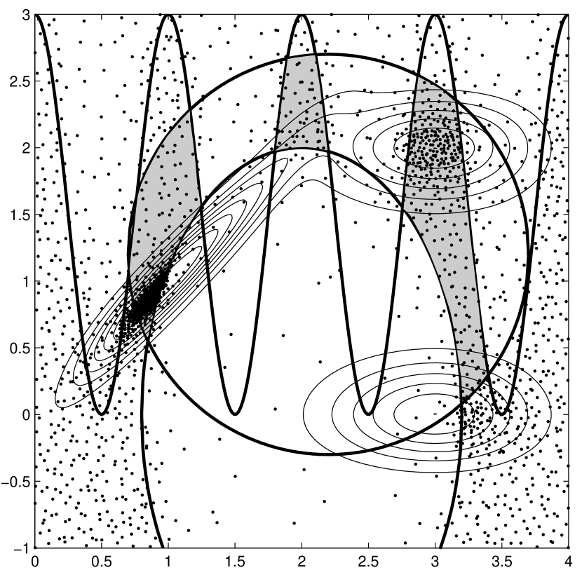
Figure 3: Trial points generated by the information algorithm combined with the penalty approach with $\delta=10^{-3}$ for Problem 1

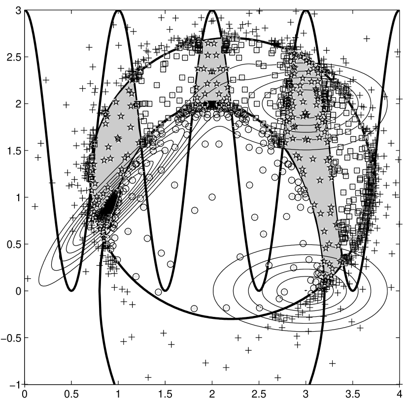
Figure 4: Trial points generated by the Strongin-Markin algorithm with $\delta=10^{-3}$ for Problem 1

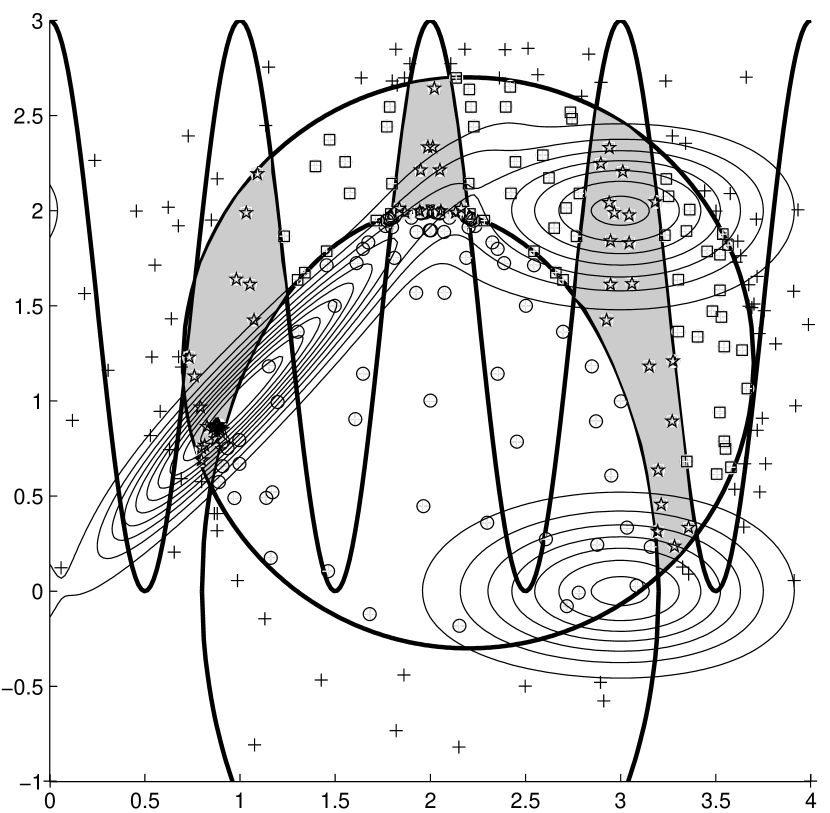
Figure 5: Trial points generated by the new algorithm with $\delta=10^{-3}$ for Problem 1

Problem 2. In this problem (see [40]) the same function as in the first experiment, over the same domain $D$, is minimized subject to the constraints

$$\begin{array}[]{l}G_{1}(y)=-(y_{1}-2.2)^{2}-(y_{2}-1.2)^{2}\leq-1.21,\\[3.0pt] G_{2}(y)=(y_{1}-2.2)^{2}+(y_{2}-1.2)^{2}\leq 1.25,\end{array}$$ (39)

that define a narrow annulus centered at the point $C\equiv(2.2,1.2)$. Here the solution is $y^{*}=(1.088,1.088)$, giving the value $\varphi(y^{*})=-1.477$ [42].

Problem 3. This is a minimization problem with four constraints (see Section 9.2 in [14]); the expression of the objective function is reported in the appendix; the search region is $D=[0,80]\times[0,80]$ and the constraints are

$$\begin{array}[]{l}G_{1}(y)=450-y_{1}y_{2}\leq 0,\\[3.0pt] G_{2}(y)=(0.1\,y_{1}-1)^{2}-y_{2}\leq 0,\\[3.0pt] G_{3}(y)=8\,(y_{1}-40)-(y_{2}-30)(y_{2}-55)\leq 0,\\[3.0pt] G_{4}(y)=(y_{1}-35)(y_{1}-30)/125+y_{2}-80\leq 0.\end{array}$$ (40)

The feasible region for this problem is connected but not convex and has a non-smooth boundary. The solution is the point $y^{*}=(77.19,64.06)$, and the value of the function at this point is $\varphi(y^{*})=-59.59$ [42].

Problem 4. The fourth test problem, proposed by the authors, is defined by the search domain $D=[0,2\,\pi]\times[0,2\,\pi]$, the non-smooth objective function

$$\varphi(y)=-|\sin(y_{1})\sin(2\,y_{2})|+0.01\,(y_{1}\,y_{2}+(y_{1}-\pi)^{2}+3\,(y_{2}-\pi)^{2})\,,$$ (41)

and the non-smooth constraints

$$\begin{array}[]{l}G_{1}(y)=1-y_{2}+\pi/2-|\sin(2\,y_{1})|+y_{1}/3\leq 0,\\[3.0pt] G_{2}(y)=y_{2}-3\,\pi/2+4\,|(\sin(y_{1}+\pi)|+y_{1}/3-1.9\leq 0.\end{array}$$

The feasible region is made of two disjoint pieces, each of which is non-convex and has a non-smooth boundary. The best solution, found by a fine grid over the search region, is $y^{*}=(1.247,2.392)$, yielding $\varphi(y^{*})=-0.864$.

Table 1: Results for Experiment 1 with $\delta=10^{-3}$

	Strongin-Markin method						New method
Problem	$n_{1}$	$n_{2}$	$n_{3}$	$n_{4}$	$n_{\varphi}$	$\varphi_{c}$	$n_{1}$	$n_{2}$	$n_{3}$	$n_{4}$	$n_{\varphi}$	$\varphi_{c}$
1	1712	953	673	-	279	-1.489	289	201	119	-	60	-1.455
2	1631	672	-	-	246	-1.477	316	142	-	-	31	-1.438
3	351	348	316	140	88	-59.59	106	103	90	65	36	-59.34
4	771	359	-	-	163	-0.864	115	60	-	-	29	-0.863

Table 2: Results for Experiments 1 with $\delta=10^{-4}$

	Strongin-Markin algorithm						New method
Problem	$n_{1}$	$n_{2}$	$n_{3}$	$n_{4}$	$n_{\varphi}$	$\varphi_{c}$	$n_{1}$	$n_{2}$	$n_{3}$	$n_{4}$	$n_{\varphi}$	$\varphi_{c}$
1	4494	2636	1487	-	826	-1.489	362	274	162	-	102	-1.489
2	4926	1941	-	-	781	-1.478	376	170	-	-	44	-1.439
3	1073	1070	1032	655	359	-59.59	115	112	99	74	45	-59.34
4	1867	787	-	-	355	-0.864	135	72	-	-	40	-0.863

In all the experiments the maximum number of iterations was set to 5000, the level of approximation of the Peano curve to $d=10$, the value $\xi$ from Step 4 to $\xi=10^{-8}$, and the value of the reliability parameter to $r=2.2$. Only the points $0$ and $1$ have been used as starting points.

In the experiments with the penalty approach the constrained problems were reduced to the unconstrained ones as follows

$$\varphi_{P}(y)=\varphi(y)+P\cdot\max\left\{G_{1}(y),G_{2}(y),\dots,G_{m}(y),0\right\},y\in D.$$

The coefficient $P$ has been computed by the rules:

– the coefficient $P$ has been chosen equal to $0.1$ for all the problems and it has been checked whether the found solution for each problem belongs or not to the feasible subregions;

– if it does not belong to the feasible subregions, the coefficient $P^{*}$ has been iteratively increased by $0.1$ until a feasible solution has been found.

Figures 3–5 present trial points generated by the three methods during Experiment 1 with $\delta=10^{-3}$. Figure 3 shows the trial points generated by the penalty approach. Remind that both the objective function and all the constraints have been evaluated at every point. Figures 4 and 5 show the points where the algorithms using the index approach have chosen to evaluate the constraints and eventually the target function. Points where the target function has been computed are denoted by stars; those where only the first constraint has been evaluated (and found violated) are denoted by crosses; circles denote points where the first constraint was satisfied and the second was not; squares denote points were the first two constraints were satisfied and the third was not.

Table 3: Results obtained by the information algorithm combined with the penalty approach Experiment 1

Test Problem	$P^{*}$	$\delta=10^{-3}$		$\delta=10^{-4}$
		$n$	$\varphi_{c}$	$n$	$\varphi_{c}$
1	$0.1$	$2298$	$-1.489$	${\bf 5000}$	$-1.489$
2	$0.3$	$428$	$-1.478$	$1621$	$-1.478$
3	$0.8$	${\bf 5000}$	$-59.59$	${\bf 5000}$	$-59.59$
4	$0.5$	$283$	$-0.864$	$789$	$-0.864$

Table 4: Speed-up obtained in Experiment 1 for Problems 1–4

Problem	1	2	3	4	1	2	3	4
	$\delta=10^{-3}$				$\delta=10^{-4}$
$S_{1}$	4.29	5.13	3.74	4.03	12.25	10.84	14.68	8.83
$S_{2}$	4.65	7.94	2.44	5.62	8.10	17.75	7.98	8.88
$S_{3}$	5.41	5.21	3.11	6.34	10.49	12.96	9.41	11.27
$\hat{S}_{1}$	7.95	1.35	47.17	2.46	13.81	4.31	43.48	5.84
$\hat{S}_{2}$	38.30	13.81	138.89	9.76	49.02	36.84	111.11	19.73
$\hat{S}_{3}$	13.74	2.63	62.50	4.16	22.47	8.24	56.18	9.58

Table 1 compares performance of the proposed algorithm to the Strongin-Markin method for $\delta=10^{-3}$. The data reported are the computed solution $\varphi_{c}$, the number of evaluations of each constraint $n_{i}$, and of the target function $n_{\varphi}$. To investigate the sensitivity of both algorithms to the value of $\delta$ the tests have been repeated with $\delta=10^{-4}$; results are reported in Table 2. Finally, Table 3 presents results obtained by the information algorithm combined with the penalty approach on Problems $1-4$, where $n$ is the number of iterations executed by the algorithm. Cases where the algorithm was not able to stop in 5000 iterations are shown in bold.

Table 4 illustrates acceleration reached by the new algorithm in comparison with the two methods tested in Experiment 1. Three speed-up indexes have been used: the first index is the ratio $S_{1}$ of iterations $n_{1}$ of the Strongin-Markin method over the new one; the second is the ratio $S_{2}$ of $n_{\varphi}$ of the objective function evaluations; finally, $S_{3}$ is the ratio of the sums $n_{\varphi}+\sum_{k=1}^{m}n_{k}$, being the number of summary evaluations of the objective function and constraints. The same quantities for the penalty approach are indicated by $\hat{S}_{i},1\leq i\leq 3$. It can be seen from Table 4 that the new method significantly outperforms both methods tested. Moreover, the computational burden increases very slowly for decreasing $\delta$ for it, while the Strongin-Markin algorithm and the penalty approach show a fast increase of iterations when a better accuracy is required.

Since Table 4 shows an evident superiority of the new method over the penalty algorithm, the latter is not used in the further experiments (also because it is difficult to determine the correct penalty coefficients for problems used in these experiments).

Experiment 2. This experiment aims at investigating the sensitivity of both algorithms to the value of the reliability parameter $r$. We have generated twenty pairs of random numbers in the range $(-1,1)$, and have added any of them to the center $C\equiv(2.2,1.2)$ of the annulus of Problem 2, thus obtaining twenty new problems, whose solutions have been found with a fine grid over the domain $D$.

They have been solved with both methods for either $r=2.5$ and $r=3$. With $r=2.5$ the proposed algorithm has found the solution in 18 cases out of 20, the Strongin-Markin algorithm was successful in 19 cases out of 20. Note that the proposed algorithm has found the solution in the case the Strongin-Markin algorithm has failed. With $r=3$, both algorithms have found the solution in all cases. The results (number of successes, average number of computation of the constraints and of the objective function) are reported in Table 5. With $r=3$, in one case the Strongin-Markin algorithm has reached the maximum number of iterations, but anyway it has found a good approximation to the solution. It can be seen from Table 5 that the computational burden increases very slowly for increasing $r$ for the proposed algorithm, while the Strongin-Markin algorithm shows a fast increase of iterations.

Table 5: Results for Experiment 2

	$r=2.5$		$r=3$
	Strongin-Markin method	New method	Strongin-Markin method	New method
Successes	$19/20$	$18/20$	$20/20$	$20/20$
$n_{1}$ average	$2177$	$359$	$2939$	$651$
$n_{2}$ average	$874$	$179$	$1150$	$330$
$n_{\varphi}$ average	$282$	$46$	$312$	$88$
$S_{1}$	–	6.06	–	4.51
$S_{2}$	–	6.13	–	3.55
$S_{3}$	–	5.71	–	4.12

Experiment 3. The last experiment involves a problem having changeable dimension $N$ and three constraints. The objective function is

$$\varphi_{N}(y)=y_{1}+e^{\rho_{N}-|\rho_{N}^{2}-5\,\rho_{N}+4|},\hskip 14.22636pt\rho_{N}=(\sum_{i=1}^{N}y_{i}^{2})^{\frac{1}{2}}.$$ (42)

The search region is $D=[-2,8]\times[-6,4]\times\ldots\times[-6,4]$ and the constraints are

$$\begin{array}[]{l}G_{1}(y)=(y_{1}-2.5)^{2}-6.25+\sum_{i=2}^{N}y_{i}^{2}\leq 0,\\[3.0pt] G_{2}(y)=-(y_{1}-2)^{2}+2.25-\sum_{i=2}^{N}y_{i}^{2}\leq 0,\\[3.0pt] G_{3}(y)=y_{2}-3\,\pi/2+4\,|(\sin(y_{1}+\pi)|+y_{1}/3+0.8\leq 0.\\[3.0pt] \end{array}$$

Numerical experiments have been executed with $2\leq N\leq 6$ with different values of $r$ and $\delta$. The level of approximation of the Peano curve was set to $d=10$ for $2\leq N\leq 5$ and to $d=8$ for $N=6$, the value $\xi=10^{-8}$. In all the experiments the maximum number of iterations was set to $40000$. The global solution is $y^{*}=(0,\ldots,0)$, yielding $\varphi_{N}(y^{*})=\exp(-4)\simeq 0.0183$.

The obtained results are shown in Tables 6 and 7. In all the experiments the new algorithm is significantly faster. It can be seen from the Table 7 that starting from dimension $N=3$ the Strongin-Markin algorithm was not able to stop in less than $40000$ iterations.

Let us comment the choice of parameters of the new method. As it has been mentioned in the Introduction, the statement of the problem does not allow to create any deterministic or stochastic algorithm that, after a finite number of evaluations of $\varphi(y)$, is able to provide an underestimate of the global minimum $\varphi(y^{*})$. These means that it is impossible to say without some additional information about the problem which values of parameters ensure that the method finds the global minimizer. However, the executed experiments can advice some recommendations.

First of all, the parameters $d$ and $\xi$ are quite technical and can be chosen easily. To have a better accuracy of the solution it is necessary to have a better approximation of the Peano curve determined by $d$. Since two points in the multidimensional space have two images at the interval $[0,1]$, then in a computer realization (see, for example, [42]) for a correct work of the method these images should be represented by two different numbers. The mapping is such that for a dimension $N$ and a level $d$ two numbers $a,b\in[0,1]$ will be considered different if $|a-b|>2^{-dN}$. For example, in double precision the minimal representable number is $2^{-52}$. Thus, if one works with a simple realization of the Peano curve using double precision, the product $dN$ should be less than $52$. Of course, more sophisticated implementations of the Peano curve realizing numbers with more digits allow to increase this number.

The second parameter is $\xi$ and it is chosen equal to a small number (see experiments). It has been introduced in the method to ensure that it works correctly in the case $l_{i}=c_{i}=r_{i}=0$ where $l_{i},c_{i},r_{i}$ are from (20). The case when the real Hölder constants are less than $\xi$ is degenerous for the method because the local tuning is not used and the method works slower.

The parameters $r$ and $\delta$ are chosen by the user on the basis of additional information about the problem or just by increasing $r$ and decreasing $\delta$ (see Table 6) trying to obtain a satisfactory result (see statement (S2) in Introduction). It can be also seen from Table 6 that by increasing dimension of the problem it is necessary to change $r$ and $\delta$ in the same way. This happens because, in spite of increasing dimension, the reduced problem is always determined over the interval $[0,1]$ independently on the dimension $N$. As a consequence, the reduced problem has more local minima, and to find the global one it is necessary to increase reliability of the method (by increasing $r$) and to make the search more accurate (by decreasing $\delta$).

Table 6: Results for the new method on Problems (42) with dimension two to six

$r$	$\delta$	$y_{1}$	$y_{2}$	$y_{3}$	$y_{4}$	$y_{5}$	$y_{6}$	$n_{1}$	$n_{2}$	$n_{3}$	$n_{\varphi}$	$\varphi_{c}$
2.35	$10^{-3}$	0.0034	0.0596	-	-	-	-	130	51	41	36	0.0295
2.35	$10^{-4}$	0.0007	0.0596	-	-	-	-	147	57	47	42	0.0268
2.45	$10^{-3}$	0.0068	0.1185	0.1182	-	-	-	819	470	377	249	0.0555
2.45	$10^{-4}$	0.0052	-0.0088	0.0107	-	-	-	5847	4723	3975	3313	0.0252
2.7	$10^{-3}$	0.2540	-0.1553	-0.0674	0.4600	-	-	708	533	364	249	0.6247
2.7	$10^{-4}$	0.0264	-0.0771	0.0400	-0.0679	-	-	14441	12485	10081	7410	0.0621
3.3	$10^{-3}$	0.5146	-0.1650	-0.0771	-0.0924	-0.3799	-	620	206	164	111	1.1704
3.3	$10^{-4}$	0.0654	0.0303	-0.2920	0.0596	-0.0692	-	18535	12289	10761	7344	0.1748
3.35	$10^{-3}$	0.5977	-0.1992	-0.0039	-0.3298	1.0898	-0.6289	445	39	35	25	1.9579
3.35	$10^{-4}$	0.3193	0.1523	-0.3945	0.1523	0.3477	0.1523	6610	2486	2292	1534	0.9688
3.35	$5\cdot 10^{-5}$	0.0508	-0.0430	0.0742	-0.0430	-0.1992	0.0504	19105	9871	8989	6233	0.1208

Table 7: Results for the Strongin-Markin algorithm on Problems (42) with dimension two to six

$r$	$\delta$	$y_{1}$	$y_{2}$	$y_{3}$	$y_{4}$	$y_{5}$	$y_{6}$	$n_{1}$	$n_{2}$	$n_{3}$	$n_{\varphi}$	$\varphi_{c}$
2.35	$10^{-3}$	0.0025	0.0010	-	-	-	-	5071	3811	3314	3066	0.0211
2.35	$10^{-4}$	0.0000	0.0010	-	-	-	-	39883	33277	31108	30423	0.0185
2.45	$10^{-3}$	0.0388	0.0010	0.0498	-	-	-	11003	5734	4911	3736	0.0654
2.45	$10^{-4}$	0.0068	0.0400	-0.0351	-	-	-	40000	22591	19901	16023	0.0320
2.7	$10^{-3}$	0.1729	0.0693	-0.1162	-0.1860	-	-	5067	1833	1680	1037	0.2676
2.7	$10^{-4}$	0.0459	0.1210	-0.2139	0.0693	-	-	40000	17699	15402	10566	0.1271
3.3	$10^{-3}$	0.5635	0.3037	-0.0381	0.3916	0.0034	-	2661	432	381	220	1.5087
3.3	$10^{-4}$	0.1436	0.3330	-0.2627	-0.0869	0.0492	-	40000	10487	9661	6137	0.3763
3.35	$10^{-3}$	0.4756	-0.2920	-0.1846	-0.0186	-0.4482	-1.1709	650	23	22	18	1.9356
3.35	$10^{-4}$	0.3877	0.1377	0.4111	0.2061	-0.3115	-0.1260	40000	5413	5091	3251	1.1450
3.35	$5\cdot 10^{-5}$	0.3877	0.1377	0.4111	0.2061	-0.3115	-0.1260	40000	5413	5091	3251	1.1450

5 Conclusions

In this paper, a novel global optimization algorithm for solving multi-dimensional Lipschitz global optimization problems with multiextremal partially defined constraints and objective function has been presented. The new algorithm uses Peano type space-filling curves and the index scheme to reduce the original constrained problem to a Hölder one-dimensional problem. Local tuning on the behaviour of the objective function and constraints is executed during the work of the global optimization procedure in order to accelerate the search. The new method works without introducing any penalty coefficients and/or auxiliary variables. Convergence conditions of a new type have been established for the algorithm.

The new algorithm enjoys the following properties:

– in order to guarantee convergence to a global minimizer $y^{*}$ it is not necessary to know the precise Lipschitz constants for the objective function and constraints for the whole search region; on the contrary, only fulfillment of condition (31) for a segment of the Peano curve containing one of the images of $y^{*}$ is required;

– the usual problem of determining the moment to stop the global procedure in order to start a local search does not arise because local information is taken into consideration throughout the duration of the global search;

– local information is taken into account not only in the neighborhood of a global minimizer but also in the whole search region, thus permitting a significant acceleration of the search;

– thanks to usage of the index scheme, the new algorithm does not introduce any additional parameters and/or variables. Constraints are evaluated at every point one at a time until the first violation of one of them, after that the rest of constraints and the objective function are not evaluated at this point. In its turn, the objective function is evaluated only for that points where all the constraints have been satisfied.

The algorithm has been tested on a number of problems taken from literature. Numerical results show the good performance of the new technique in comparison with the two methods taken from literature.

Appendix

The target function for Problem 3 is

$$\begin{array}[]{ll}\varphi(y)=&-(B_{1}+B_{2}\,y_{1}+B_{3}\,y_{1}^{2}+B_{4}\,y_{1}^{3}+B_{5}\,y_{1}^{4}+B_{6}\,y_{2}+B_{7}\,y_{1}y_{2}+B_{8}\,y_{1}^{2}y_{2}\\[3.0pt] &+\,B_{9}\,y_{1}^{3}y_{2}+B_{10}\,y_{1}^{4}y_{2}+B_{11}\,y_{2}^{2}+B_{12}\,y_{2}^{3}+B_{13}\,y_{2}^{4}+B_{14}/(1+y_{2})\\[3.0pt] &+\,B_{15}\,y_{1}^{2}y_{2}^{2}+B_{16}\,y_{1}^{3}y_{2}^{2}+B_{17}\,y_{1}^{3}y_{2}^{3}+B_{18}\,y_{1}y_{2}^{2}+B_{19}\,y_{1}y_{2}^{3}\\[3.0pt] &+\,B_{20}\exp(0.0005\,y_{1}y_{2}))\end{array}$$

where coefficients $B_{1},\ldots,B_{20}$ are

$B_{1}=75.1963666677;B_{2}=-3.8112755343;B_{3}=0.1269366345;B_{4}=-0.0020567665;\\ B_{5}=0.0000103450;B_{6}=-6.8306567613;B_{7}=0.0302344793;B_{8}=-0.0012813448;\\ B_{9}=0.0000352559;B_{10}=-0.0000002266;B_{11}=0.2564581253;B_{12}=-0.0034604030;\\ B_{13}=0.0000135139;B_{14}=-28.1064434908;B_{15}=-0.0000052375;B_{16}=-0.0000000063;\\ B_{17}0=0.0000000007;B_{18}=0.0003405462;B_{19}=-0.0000016638;B_{20}=-2.8673112392.$

References

- [1] V. Balakrishnan and S. Boyd. Global optimization in control system analysis and design. In E. Leondes, editor, Control and Dynamic Systems, volume 53, pages 1–55. Academic Press, 1993.
- [2] D. Bertsimas and M. Grigni. Worst case examples for the spacefilling curve heuristic for the euclidean traveling salesman problem. Operations Research Letters, 8:241–244, 1989.
- [3] V. Blondel and J. N. Tsitsiklis. -hardness of some linear control design problems. SIAM J. Control Optim., 35:2118–2127, 1997.
- [4] I.M. Bomze, T. Csendes, R. Horst, and P.M. Pardalos. Developments in Global Optimization. Kluwer Academic Publishers, Dordrecht, 1997.
- [5] A.R. Butz. Space filling curves and mathematical programming. Information and Control, 12(4):313–330, 1968.
- [6] S. A. Crivelli, T. Head-Gordon, R. H. Byrd, E. Eskow, and R. B. Schnabel. A hierarchical approach for parallelization of a global optimization method for protein structure prediction. In Proc. of Euro-Par 1999, pages 578–585, Berlin, 1999. Springer Verlag.
- [7] D. Famularo, P. Pugliese, and Ya. D. Sergeyev. A global optimization technique for checking parametric robustness. Automatica, 35:1605–1611, 1999.
- [8] C. A. Floudas and P. M. Pardalos. Optimization in Computational Chemistry and Molecular Biology: Local and Global Approaches. Kluwer Academic Publishers, Dordrecht, 2000.
- [9] E. Gourdin, B. Jaumard, and R. Ellaia. Global optimization of Hölder functions. J. Global Optim., 8:323–348, 1996.
- [10] I. E. Grossman. Global Optimization in Engineering Design. Kluwer Academic Publishers, Dordrecht, 1996.
- [11] E. R. Hansen. Global Optimization Using Interval Analysis. Marcel Dekker, New York, 1992.
- [12] P. Hansen and B. Jaumard. Lipschitz optimization. In R. Horst and P.M. Pardalos, editors, Handbook of Global Optimization, pages 278–282. Kluwer Academic Publishers, Dordrecht, 1995.
- [13] D. Hilbert. Über die steitige abbildung einer linie auf ein flächenstück. Mathematische Annalen, 38:459–460, 1891.
- [14] D. M. Himmelblau. Applied Nonlinear Programming. McGraw-Hill, New York, 1972.
- [15] R. Horst and P. M. Pardalos. Handbook of Global Optimization. Kluwer Academic Publishers, Dordrecht, 1995.
- [16] D.R. Jones, C.D. Perttunen, and B.E. Stuckman. Lipschitzian optimization without the Lipschitz constant. J. Optimization Theory Appl., 79(1):157–181, 1993.
- [17] R. B. Kearfott. Rigorous Global Search: Continuous Problems. Kluwer Academic Publishers, Dordrecht, 1996.
- [18] C. T. Kelley. Iterative Methods for Optimization. SIAM, Philadelphia, 1999.
- [19] D. Lera and Ya. D. Sergeyev. Global minimization algorithms for Hölder functions. BIT, 42(1):119–133, 2002.
- [20] J. Mockus, W. Eddy, A. Mockus, L. Mockus, and G. Reklaitis. Bayesian Heuristic Approach to Discrete and Global Optimization: Algorithms, Visualization, Software, and Applications. Kluwer Academic Publishers, Dordrecht, 1996.
- [21] A. Nemirovskii. Several -hard problems arising in robust stability analysis. Math. Control Signal Systems, 6:99–105, 1993.
- [22] P. M. Pardalos, E. Romeijn, and H. Tuy. Recent developments and trends in global optimization. J. Comput. Appl. Math., 124(1–2):209–228, 2000.
- [23] P. M. Pardalos, D. Shalloway, and G. Xue. Global Minimization of Nonconvex Energy Functions: Molecular Conformation and Protein Folding. American Mathematical Society, DIMACS, AMS, 1996.
- [24] G. Peano. Sur une courbe, qui remplit toute une aire plane. Mathematische Annalen, 36:157–160, 1890.
- [25] J. Pintér. Global Optimization in Action (Continuous and Lipschitz Optimization: Algorithms, Implementations and Applications. Kluwer Academic Publishers, Dordrecht, 1996.
- [26] L. K. Platzman and J. J. Bartholdi III. Spacefilling curves and the planar travelling salesman problem. J. ACM, 36(4):719–737, 1989.
- [27] H. Ratschek and J. Rokne. New Computer Methods for Global Optimization. Ellis Horwood, Chichester, 1988.
- [28] K. Ritter. Average-Case Analysis of Numerical Problems. Springer Verlag, Berlin, 2000.
- [29] H. Sagan. Space-Filling Curves. Springer Verlag, Berlin, 1994.
- [30] M. K. Sen and P. L. Stoffa. Global Optimization Methods in Geophysical Inversion. Elsevier, Amsterdam, 1995.
- [31] Ya. D. Sergeyev. An information global optimization algorithm with local tuning. SIAM J. Optim., 5:858–870, 1995.
- [32] Ya. D. Sergeyev. Global one-dimensional optimization using smooth auxiliary functions. Mathematical Programming, 81(1):127–146, 1998.
- [33] Ya. D. Sergeyev. On convergence of ”divide the best” global optimization algorithms. Optimization, 44(3):303–325, 1998.
- [34] Ya. D. Sergeyev, P. Daponte, D. Grimaldi, and A. Molinaro. Two methods for solving optimization problems arising in electronic measurements and electrical engineering. SIAM J. Optim., 10(1):1–21, 1999.
- [35] Ya. D. Sergeyev and D. L. Markin. An algorithm for solving global optimization problems with nonlinear constraints. J. Global Optimiz., 7:407–419, 1995.
- [36] C.-S. Shao, R. Byrd, E. Eskow, and R. B. Schnabel. Global optimization for molecular clusters using a new smoothing approach. J. Global Optimiz., 16(2):167–196, 2000.
- [37] C. P. Stephens and W. P. Baritompa. Global optimization requires global information. J. Optimization Theory Appl., 96(3):575–588, 1998.
- [38] R. G. Strongin. Numerical Methods in Multi-Extremal Problems (Information-Statistical Algorithms). Nauka, Moscow, 1978, (In Russian).
- [39] R. G. Strongin. Numerical methods for multiextremal nonlinear programming problems with nonconvex constraints. In V.F. Demyanov and D. Pallaschke, editors, Lecture Notes in Economics and Mathematical Systems, volume 255, pages 278–282. Springer Verlag, Laxenburg, 1985.
- [40] R. G. Strongin. Algorithms for multi-extremal mathematical programming problems employing the set of joint space-filling curves. Journal of Global Optimization, 2:357–378, 1992.
- [41] R. G. Strongin and D. L. Markin. Minimization of multiextremal functions with nonconvex constraints. Cybernetics, 22:486–493, 1986.
- [42] R. G. Strongin and Ya. D. Sergeyev. Global Optimization with Non-Convex Constraints: Sequential and Parallel Algorithms. Kluwer Academic Publishers, Dordrecht, 2000.
- [43] The MathWorks, Inc. Using MATLAB. Natick, MA., 1996.
- [44] A. Törn and A. Z̆ilinskas. Global Optimization. Springer Verlag, Berlin, 1989.
- [45] R. J. Vanderbei. Extension of Piyavskii’s algorithm to continuous global optimization. J. Global Optimiz., 14:205 –216, 1999.
- [46] A. A. Zhigljavsky. Theory of Global Random Search. Kluwer Academic Publishers, Dordrecht, 1991.