Dynamics of two topologically entangled chains

Abstract

Starting from a given topological invariant, we argue that it is possible to construct a topological field theory with a finite number of Feynman diagrams and an amplitude of gauge invariant objects that is a function of that invariant. This is for example the case of the Gauss linking number and of the abelian BF models which has been already successfully applied in the statistical mechanics of polymers. In this work it is shown that a suitable generalization of the BF model can be applied also to polymer dynamics, where the polymer trajectories are not static, but change their shape during time.

I Introduction

There are many situations in which it is necessary to consider topological relations among one-dimensional objects that are homeomorphic to rings. The most significant examples are provided by long flexible polymers and biopolymers, whose trajectories may close themselves and form what in the polymer scientific literature are called catenanes wasser –ff . The latter are able to entangle themeselves giving rise to complex links involving two or more interlocked chains. Additionally, each catenanae may be in the configuration of a nontrivial knot. Two cases of polymer links are shown in Fig. 1.

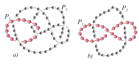
Figure 1: Entangled polymers rings $P_{1}$ and $P_{2}$ with linked trajectories $C_{1}$ and $C_{2}$. In a) polymer $P_{2}$ is in a nontrivial knot configuration, while in b) both trajectories are unknots.

Besides polymers, other examples in which topological relations among a system of one-dimensional objects become relevant can be found in condensed matter physics (paths around defects in melted crystals) chaikin ; pieranski or in particle physics (loops in quantum gravity and the so-called hopfions) ash ; smolin ; hopfions . In order to specify the topological states of a given system of this kind one uses knots or link invariants. In the following, we will be interested in the topological relations of a system of a linked rings without taking into account the fact that these rings could be also in a nontrivial knot configuration as for example in Fig. 1 a). For this reason, we will discuss here only link invariants.

It is well known that the correlation functions of the observables of a topological field theory are topological invariants. Moreover, the coefficients of the perturbative expansion of those correlation functions are topological invariants too. In practice, this means that to a finite set of Feynman diagrams it is possible to associate a given topological invariant. Our purpose is to solve the inverse problem. This means that, starting from a given topological invariant, we would like to obtain a topological field theory with a finite set of Feynman diagrams and a correlation function which is a function of that invariant. This is the program of topological engineering that has been stated in Ref. ffbookch . In the last few decades topological theories with the above characteristics have been extensively applied in the statistical mechanics of polymers, see for instance edwards –ferrariTFT and ffbookch ; leal . The most popular approach used in order to distinguish the different topological configurations of the one-dimensional objects is based on the Gauss linking number (GLN). The corresponding topological field theory is an abelian BF model discussed in Ref. blau . The goal of this work is to extend this approach based on the GLN to the case of polymer dynamics, in which the shape of the linked trajectories is not static, but changes in time.

II The topological engineering program

The program of topological engineering in the case of links may be summarized as follows:
Let $\cal{T}(\ell)$ be a link invariant, which describes the topological properties of a $N$–component link $\ell$. It is required that:

• the invariant $\cal{T}(\ell)$ is explicitly written as a functional of trajectories $C_{1},\ldots,C_{N}$ of knots composing the link.
  Given a link invariant of this kind, find a topological field theory with observables ${\cal{O}}_{1},\ldots,{\cal{O}}_{n}$ such that $\cal{T}(\ell)$, or equivalently a function $F[\cal{T}(\ell)]$ of it, can be expressed as the correlator of these observables

  $$F({\cal{T}})=\int\!{\cal{D}}\{\phi\}e^{-S(\{\phi\})}{\cal{O}}_{1}(\{\phi\}),\ldots,{\cal{O}}_{n}(\{\phi\})$$ (1)

  where $S(\{\phi\})$ is the action of a system and $\{\phi\}$ is a set of fields that can be scalars, vectors or higher order tensors.

The topological field theory and its observables should satisfy the following conditions:

• Each observable ${\cal{O}}_{i}$, $i=1,\ldots,n$, must depend on the trajectory of only one knot

• No further regularization should be necessary in order to compute the correlator $\langle{\cal O}_{1},\ldots,{\cal O}_{n}\rangle$, apart from the usual regularization schemes required by the possible presence of ultraviolet divergences.

An example of topological engineering is based on the GLN and the abelian BF field theory. The GLN is given by:

$$\chi(C_{1},C_{2})=\frac{1}{4\pi}\epsilon_{\mu\nu\rho}\oint_{C_{1}}\!dx_{1}^{\mu}(s_{1})\oint_{C_{2}}\!dx_{2}^{\nu}(s_{2})\frac{(x_{1}(s_{1})-x_{2}(s_{2}))^{\rho}}{|x_{1}(s_{1})-x_{2}(s_{2})|^{3}}$$ (2)

where $x_{1}(s_{1})^{\mu}$ and $x_{2}(s_{2})^{\nu}$ are spatial curves in three dimensions that represent respectively the closed trajectories $C_{1}$ and $C_{2}$ of two polymers $P_{1}$ and $P_{2}$. The Greek indexes $\mu,\nu,\rho=1,2,3$ denote the spatial components. Here $s_{1}$ and $s_{2}$ represent the arc-lengths on the curves $C_{1}$ and $C_{2}$. $s_{1}$ and $s_{2}$ are defined in a such a way that $0\leq s_{1}\leq L$ and $0\leq s_{2}\leq L$. To find a field theory which is associated to the invariant $\chi(C_{1},C_{2})$, we rewrite (2) as follows

$$\chi(C_{1},C_{2})=\int\!d^{3}x\int\!d^{3}y\xi_{1}^{\mu}(x)G_{\mu\nu}(x-y)\xi_{2}^{\nu}(y)$$ (3)

where

$$\xi_{1}^{\mu}(x)=\oint_{C_{1}}\!dx_{1}^{\mu}\delta(x-x_{1})\qquad\xi_{2}^{\nu}(x)=\kappa\oint_{C_{2}}\!dx_{2}^{\nu}\delta(x-x_{2})$$ (4)

are called the bond vectors densities and

$$G_{\mu\nu}(x-y)=\frac{1}{2\pi\kappa}\epsilon_{\mu\nu\rho}\frac{(x-y)^{\rho}}{|x-y|^{3}}$$ (5)

Let us note that $G_{\mu\nu}(x-y)$ coincides with the propagator of the abelian BF model discussed in Ref. blau . To make the connection with the BF model even more explicit, we have introduced a new parameter $\kappa$, which will play later the role of the coupling constant of that model. Clearly, the addition of this parameter is irrelevant. As a matter of fact, the right hand side of Eq. (3) does not depend on $\kappa$. Now the quantity

$$e^{i\chi(C_{1},C_{2})}=e^{i\int\!d^{3}x\int\!d^{3}y\xi_{1}^{\mu}(x)G_{\mu\nu}(x-y)\xi_{2}^{\nu}(y)}$$ (6)

can be regarded as the generating functional of a Gaussian field theory with propagator $G_{\mu\nu}(x-y)$ for the very special choice of currents (4). It is easy to recognize that the underlaying field theory is an Abelian BF model with action

$$S_{\mbox{\tiny BF}}=i\kappa\epsilon^{\mu\nu\rho}\int\!d^{3}xA_{\mu}\partial_{\nu}B_{\rho}$$ (7)

It is possible to show that the abelian version of the BF model is actually equivalent to two Abelian C-S field theories. If we quantize the above topological field theory using the Lorentz gauge fixing, in which both fields $A_{\mu}$ and $B_{\mu}$ are completely transverse, we obtain the following relation

$$e^{i\chi(C_{1},C_{2})}=\int\!{\cal D}A_{\mu}{\cal D}B_{\mu}e^{-S_{\mbox{\tiny BF}}}e^{i\int\!d^{3}x\xi_{1}^{\mu}A_{\mu}}e^{i\kappa\int\!d^{3}x\xi_{2}^{\mu}B_{\mu}}\delta(\partial^{\mu}A_{\mu})\delta(\partial^{\mu}B_{\mu})$$ (8)

The above equation is the analog of Eq. (1) in the present case. There are just two observables ${\cal O}_{1}$ and ${\cal O}_{2}$, namely the two Abelian Wilson loops given below:

$${\cal O}_{1}=e^{i\int\!d^{3}x\xi_{1}^{\mu}A_{\mu}}\qquad{\cal O}_{2}=e^{i\kappa\int\!d^{3}x\xi_{2}^{\mu}B_{\mu}}$$ (9)

III The case of dynamics

In this Section we would like to extend the program of topological engineering to the case of two trajectories whose configurations are changing during time. This problem is very important to study the dynamics of two entangled polymers. Once again, we choose the Gauss linking invariant in order to impose topological conditions on two closed trajectories $C_{1}$ and $C_{2}$. The only difference from the previous static example is that now the curves $x_{1}$ and $x_{2}$ depend on time, i.e. $x_{1}=x_{1}(t,s_{1})$ and $x_{2}=x_{2}(t,s_{2})$. The GLN can still be defined, but will be a time dependent quantities:

$$\chi(t,C_{1},C_{2})=\frac{1}{4\pi}\epsilon_{\mu\nu\rho}\oint_{C_{1}}\!dx_{1}^{\mu}(t,s_{1})\oint_{C_{2}}\!dx_{2}^{\nu}(t,s_{2})\frac{(x_{1}(t,s_{1})-x_{2}(t,s_{2}))^{\rho}}{|x_{1}(t,s_{1})-x_{2}(t,s_{2})|^{3}}$$ (10)

Of course, if the trajectories would be impenetrable, then $\chi$ would be a constant, since it is not possible to change the topological configuration of a system of knots if their trajectories are not allowed to cross themselves. However, in the absence of excluded volume interactions models of polymer physics are phantom, i.e. crossings are allowed. For this reason, we will require that only the time average of the GLN is fixed. As a consequence, we will consider a time averaged version of the GLN on the time interval $[0,t_{f}]$:

$$\langle\chi(t,C_{1},C_{2})\rangle=\int_{0}^{t_{f}}\frac{dt}{t_{f}}\chi(t,C_{1},C_{2})$$ (11)

Next, we generalize Eq. (6) to the case of dynamics. To this purpose, we introduce the following field theory

$$S=\frac{1}{t_{f}}\epsilon_{\mu\nu\rho}\int\!d\eta d^{3}xA^{\mu}(\eta,x)\partial_{x}^{\nu}B^{\rho}(\eta,x)$$ (12)

The above action differs from that of Eq. (7) by the addition of the fourth dimension represented by variable $\eta$, with $-\infty<\eta<+\infty$. Note that $S$ is not invariant under diffeomorphism on the whole dimensional space spanned by the coordinates $x^{1},x^{2},x^{3}$ and $\eta$, but only on its three dimensional spatial section. As a consequence, strictly speaking $S$ does not describe a topological field theory. The propagator corresponding to the action (12) in the Lorentz gauge is given by

$$G_{\mu\nu}(\eta,\eta^{\prime};x,x^{\prime})=\frac{t_{f}}{2\pi}\epsilon_{\mu\nu\rho}\frac{(x-x^{\prime})^{\rho}}{|x-x^{\prime}|^{3}}\delta(\eta-\eta^{\prime})$$ (13)

The analog of Eq. (6) is

$$e^{-i\lambda\chi(C_{1},C_{2})}=\int\!{\cal{D}}A_{\mu}{\cal{D}}B_{\nu}e^{-iS}e^{-i\int\!d\eta d^{3}x(J_{1}^{\mu}(\eta,x)A_{\mu}(\eta,x)+J_{2}^{\mu}(\eta,x)B_{\mu}(\eta,x))}$$ (14)

where

$$J_{1}^{\mu}(\eta,x)=\frac{1}{2t_{f}}\int_{0}^{t_{f}}\!\frac{dt}{t_{f}}\delta(\eta-t)\int_{0}^{L_{1}}\!ds_{1}\frac{\partial}{\partial s_{1}}x_{1}^{\mu}(t_{1},s_{1})\delta^{(3)}(x-x_{1}(t,s_{1}))$$ (15)

and

$$J_{2}^{\mu}(\eta,x)=\lambda\int_{0}^{t_{f}}\!\frac{dt}{t_{f}}\delta(\eta-t)\int_{0}^{L_{2}}\!ds_{2}\frac{\partial}{\partial s_{2}}x_{2}^{\mu}(t_{1},s_{2})\delta^{(3)}(x-x_{2}(t,s_{2}))$$ (16)

The right hand side of Eq. (14) can be seen as the amplitude of the two observables

$${\cal O}_{1}=e^{-i\int\!d\eta d^{3}xJ_{1}^{\mu}(\eta,x)A_{\mu}(\eta,x)}\qquad{\cal O}_{2}=e^{-i\int\!d\eta d^{3}xJ_{2}^{\mu}(\eta,x)B_{\mu}(\eta,x)}$$ (17)

To prove Eq. (14) it is sufficient to perform the Gaussian integration in the fields $A^{\mu}$ and $B^{\mu}$. The result of that operation is

$$e^{-i\int\!d\eta d^{3}x(J_{1}^{\mu}(\eta,x)A_{\mu}(\eta,x)+J_{2}^{\mu}(\eta,x)B_{\mu}(\eta,x))}=e^{-i\int\!d\eta d^{3}x\int\!d\eta^{\prime}d^{3}x^{\prime}J_{1}^{\mu}(\eta,x)G_{\mu\nu}(\eta,\eta^{\prime};x,x^{\prime})J_{2}^{\nu}(\eta^{\prime},x^{\prime})}$$ (18)

Using the explicit expression of the propagator $G_{\mu\nu}(\eta,\eta^{\prime};x,x^{\prime})$ given in Eq. (13) it is possible to verify Eq. (14) after eliminating the spurious variables $\eta,\eta^{\prime}$ and $x,x^{\prime}$:

$$e^{-i\int\!d\eta d^{3}x\int\!d\eta^{\prime}d^{3}x^{\prime}J_{1}^{\mu}(\eta,x)G_{\mu\nu}(\eta,\eta^{\prime};x,x^{\prime})J_{2}^{\nu}(\eta^{\prime},x^{\prime})}=$$ (19)

$$\!\!\!\!\!\!\exp{\left[-\frac{i\lambda}{4\pi}\int_{0}^{t_{f}}\!\frac{dt}{t_{f}}\int_{0}^{L_{1}}\!ds_{1}\int_{0}^{L_{2}}\!ds_{2}\epsilon_{\mu\nu\rho}\frac{\partial}{\partial s_{1}}x_{1}^{\mu}(t,s_{1})\frac{\partial}{\partial s_{2}}x_{2}^{\nu}(t,s_{2})\frac{(x_{1}(t,s_{1})-x_{2}(t,s_{2}))^{\rho}}{|(x_{1}(t,s_{1})-x_{2}(t,s_{2})|^{3}}\right]}$$

The right hand side of above equation coincides with $e^{-i\lambda\chi(C_{1},C_{2})}$. This completes our proof.

IV Concluding remarks

In this work the program of topological engineering has been extended to the case of the dynamics of two polymer chains. In particular, the Gauss linking invariant has been considered. It has been shown that a time average version of this topological invariant can be reproduced from an amplitude of a field theory in the form of Eq. (1). This amplitude is given in Eq. (14). Due to the fact that the conformations of the chains change during time, the underlying field theory is four dimensional and it is topological only with respect to diffeomorphisms of the spatial section of four dimensional space.

V Acknowledgments

One of us – M. Pia̧tek – would like to thank the University of Szczecin and the Faculty of Mathematics and Physics of that University for the kind hospitality.

References

- (1) E. Wasserman, Jour. Am. Chem. Soc. 82, 4433 (1960).
- (2) S.A. Wasserman and N.R. Cozzarelli, Science 232, 951 (1986).
- (3) N.C. Seeman et al., New J. Chem. 17, 739 (1993).
- (4) D.E. Adams, E.M. Shekhtman, E.L. Zechiedrich, M.B. Schmid and N.R. Cozzarelli, Cell 71, 277 (1992).
- (5) S.D. Levene, C. Donahue, T.C. Boles and N.R. Cozzarelli Biophys. J. 69 1036, (1995).
- (6) Molecular Catenanes, Rotaxanes and Knots: A Journey Through the World of Molecular Topology, J.-P. Sauvage and C. Dietrich-Buchecker (Eds.) (Wiley, 1999).
- (7) G. Ten Brinke and G. Haziioannou, Macromolecules 20, 480 (1987).
- (8) A. Vologodskii and V.V. Rybenkov, Phys. Chem. Chem. Phys. 11, 10543 (2009).
- (9) S.F. Edwards, Proc. Phys. Soc. 91, 513 (1967); J. Phys. A (Proc. Phys. Soc.) 1, 15 (1968).
- (10) M.G. Brereton and S. Shah, J. Phys. A:Math. Gen. 13, 2751 (1980); J. Phys. A:Math. Gen. 15, 985 (1982).
- (11) F. Tanaka, Prog. Theor. Phys. 68, 164 (1982); Prog. Theor. Phys. 68, 148 (1982).
- (12) M.G. Brereton and T.A. Vilgis, J. Phys. A: Math. Gen. 28, 1149 (1995).
- (13) M.G. Brereton, J. Phys. A: Math Gen. 34, 5131 (2001).
- (14) T.A. Vilgis and H.L. Frisch, Polymer Bulletin 21, 655 (1989).
- (15) M. Otto and T.A. Vilgis, Phys. Rev. Lett. 80, 881 (1998).
- (16) M. Otto, J. Phys. A: Math. Gen. 34, 2539 (2001); J. Phys. A: Math. Gen. 37, 2881 (2004).
- (17) F. Ferrari, Ann. Phys. (Leipzig) 11 4, 255 (2002); F. Ferrari and I. Lazzizzera Nucl. Phys. B 559 (3), 673 (1999).
- (18) F. Ferrari, H. Kleinert, and I. Lazzizzera, Int. Jour. Mod. Phys. B 14 (32), 3881 (2000); Phys. Lett. A 276, 31 (2000).
- (19) Principles of Condensed Matter Physics, P.M. Chaikin and T.C. Lubensky, (Cambridge, 1995).
- (20) P. Pierański, Eur. Phys. Lett. 81, 66001 (2008).
- (21) A. Ashtekar, Phys. Rev. Lett. 57 18, 2244 (1986).
- (22) C. Rovelli and L. Smolin, Phys. Rev. Lett. 61, 1155 (1988); Nucl. Phys. B331, 80 (1990).
- (23) L. D. Faddeev and A. J. Niemi, Knots and particles, Nature 387 (58) (1997), [arXiv:hep-th/9610193].
- (24) F. Ferrari, Topological field theories with non-semisimple gauge group of symmetry and engineering of topological invariants, in Trends in Field Theory Research, O. Kovras (Ed.) (Nova Science Publisher 2004).
- (25) L. Leal and J. Pineda, Mod. Phys. Lett. A 23, 205 (2008).
- (26) M. Blau and G. Thompson, Ann. Phys. (NY) 205, 130 (1991).