$\Lambda$CDM , $\Lambda$DGP and extended phantom-like cosmologies

Abstract

In this paper we compare outcomes of some extended phantom-like cosmologies with each other and also with $\Lambda$CDM  and $\Lambda$DGP. We focus on the variation of the luminosity distances, the age of the universe and the deceleration parameter versus the redshift in these scenarios. In a dynamical system approach, we show that the accelerating phase of the universe in the $f(R)$-DGP scenario is stable if one consider the curvature fluid as a phantom scalar field in the equivalent scalar-tensor theory, otherwise it is a transient and unstable phenomenon. Up to the parameters values adopted in this paper, the extended $F(R,\varphi)$-DGP scenario is closer to the $\Lambda$CDM scenario than other proposed models. All of these scenarios explain the late-time cosmic speed-up in their normal DGP branches, but the redshift at which transition to the accelerating phase occurs are different: while the $\Lambda$DGP model transits to the accelerating phase much earlier, the $F(R,\varphi)$-DGP model transits to this phase much later than other scenarios. Also, within the parameter spaces adopted in this paper, the age of the universe in the $f(R)$-DGP model is larger than $\Lambda$CDM, but this age in $F(G,\varphi)$-DGP is smaller than $\Lambda$CDM.

1 Introduction

One of the most remarkable discoveries of the past decade is that the universe is currently in an accelerating phase, which means that expanding velocity of the universe is increasing. This phenomenon is supported by data related to the luminosity measurements of high red shift supernovae (Perlmutter, 1999; Riess, 1998; Astier et al., 2006; Wood-Vasey et al., 2007), measurement of degree-scale anisotropies in the cosmic microwave background (CMB) (Miller et al., 1999; Hanany, 2000; Spergel et al., 2003) and large scale structure (LSS) (Colless et al., 2001; Tegmark et al., 2004; Cole et al., 2005; Springel et al., 2006). The rigorous treatment of this phenomenon can be provided in the framework of general relativity. In the expression of general relativity, late time acceleration can be explained either by an exotic fluid with large negative pressure that is dubbed as dark energy in literature, or by modifying the gravity itself which is dubbed as dark geometry or dark gravity proposal. The first and simplest candidate of dark energy is the cosmological constant, $\Lambda$ (Sahni & Wang, 2000; Padmanabhan, 2003; Copeland et al., 2006). But there are theoretical problems associated with it, such as its unusual small numerical value ( the fine tuning problem), no dynamical behavior and its unknown origin (Weinberg, 1989; Carroll, 2001; Caldwell et al., 1999). These problems have forced cosmologists to introduce alternatives in which dark energy evolves during the universe evolution. Scalar field models with their specific features provide an interesting alternative for cosmological constant and can reduce the fine tuning and coincidence problems. In this respect, several candidate models have been proposed: ”quintessence” scalar field (Ratra & Peebles, 1988; Saini et al., 2000; Brax & Martin, 2000; Barreiro et al., 2000; Sahni & Wang, 2000; Sahni et al., 2002; Sami & Padmanabhan, 2003), phantom fields (Caldwell, 2002; Tsujikawa & Sami, 2004; Caldwell & Linder, 2005; Cai et al., 2010; Moyassari & Setare, 2009) and chaplygin gas (Kamenshchik et al., 2001; Dev et al., 2003; Amendola et al., 2003; Roos, 2007; Bouhmadi-López & Lazkoz, 2007; Zhang et al., 2006a; Zhang & Zhu, 2006b; Bertolami et al., 2004; Biesiada et al., 2005; Heydari-Fard & Sepangi, 2008; Roos, 2008a, b; Zhang et al., 2009; Setare, 2009) are among these candidates.

As an alternative for dark energy, modification of gravity can be accounted for the late time acceleration. Among the most popular modified gravity scenarios which may successfully describe the cosmic speed-up, is $f(R)$ gravity (Capozziello, 2003; Sotiriou, 2010; Nojiri & Odintsov, 2003, 2004, 2005, 2006; Nojiri et al., 2007; Nojiri & Odintsov, 2008; Bamba et al., 2008; Carroll et al., 2004; Amendola et al., 2007; Nozari, 2008a; Atazadeh et al, 2008; Saavedra & Vasquez, 2009; Setare, 2008). Modified gravity also can be achieved by extra-dimensional theory in which the observable universe is a 4-dimensional brane embedded in a five-dimensional bulk. Dvali- Gabadadze-Porrati (DGP) model is one of the extra-dimensional models that can describe late-time acceleration of the universe in its self-accelerating branch due to leakage of gravity to the extra dimension (Dvali et al., 2000a, b; Dvali & Gabadadze, 2001; Dvali et al., 2002; Deffayet, 2001; Lue, 2006).

Recent observations constrain the equation of state parameter of the dark energy to be $\omega_{X}\approx-1$ and even $\omega_{X}<-1$ (Melchiorri et al., 2003; Riess et al., 2004; Komatsu et al., 2009). One of the candidates for dark energy of this kind is the phantom scalar field. This component has the capability to create the mentioned acceleration and its behavior is extremely fitted to observations. But it suffers from problems; it violates the null energy condition and its energy density increases with expansion of the universe which is an unphysical behavior. Also it causes the quantum vacuum instabilities. So, cosmologists have tried to realize a kind of phantom-like behavior in the cosmological models without introduction of phantom fields (Sahni & Shtanov, 2003; Sahni, 2004; Shtanov, 2000; Lue & Starkman, 2004). With phantom mimicry ( the phantom-like behavior), effective equation of state parameter of dark component remains less than $-1$ and effective energy density of the unverse increases with cosmic expansion. In the framework of general relativity these two expressions are equivalent. However, in the effective picture of cosmological models, in order to satisfy phantom-like behavior, the mentioned two expressions must be investigated separately. The phantom mimicry discussed in this study has a geometric origin. In this paper, we discuss briefly DGP-inspired theoretical models that realize phantom-like behavior. We present cosmological dynamics in each proposed model and then we compare these models with $\Lambda$CDM and also with each other through investigation of their expansion histories. Within a dynamical system ( phase space) approach, we show that the accelerating phase of the universe in the $f(R)$-DGP scenario is stable if one consider the curvature fluid as a phantom scalar field in the equivalent scalar-tensor theory, otherwise it is a transient and unstable phenomenon. As another important probe, we study the age of the universe in each model. We show that some of these models account for a transient accelerated phase.

2 The phantom-like evolution

As we have pointed out in the introduction, the observational evidences show that the equation of state parameter of dark energy in the universe can be less than $-1$. Many attempts have been made to find dark energy models that allow the so-called phantom dark energy: a dark energy component with large negative pressure and negative kinetic energy with equation of state parameter less than $-1$. A phantom field is described by the following action

$$S=\int\Big{[}\frac{1}{2}g^{\mu\nu}\partial_{\mu}\varphi\partial_{\nu}\varphi-V(\varphi)\Big{]}\sqrt{-g}d^{4}x\,,$$ (1)

The kinetic energy term of the phantom field in the corresponding lagrangian enters with opposite sign in contrast to the ordinary matter and this distinguishes phantom field from ordinary (canonical) fields. But this distinctive property of the phantom field causes a series of quantum vacuum instabilities. Also, due to characteristic $p<-\rho$ feature of this kind of matter, it violates the null energy condition. On the other hand, dark energy with $\omega<-1$ (phantom energy) is beset with a host of undesirable properties which makes this model of dark energy to be unattractive. So, cosmologists attempted to find a way which removes these problems. They are forced to consider models that realize phantom-like behavior without introducing any phantom matter. In the language of general relativity, phantom-like behavior means that the equation of state parameter of dark energy is less than $-1$ or its energy density increases with expansion of the universe. In the cosmological models that there is no phantom matter, two mentioned expressions for the phantom-like behavior are not equivalent and should be investigated separately.

3 Phantom mimicry: extended models

3.1 $\Lambda$CDM vs $\Lambda$DGP

A cosmological model which has the capability to realize the phantom-like behavior without introducing any phantom matter, is the $\Lambda$DGP model. Firstly, we introduce briefly the $\Lambda$DGP model. The DGP model, as a modified theory of gravity that modifies the geometric sector of the Einstein field equations, has a modified Friedmann equation as follows (Dvali et al., 2000a; Deffayet, 2001; Lue, 2006)

$$H^{2}\pm\frac{H}{r_{c}}=\frac{8\pi G}{3}\rho(t)\,,$$ (2)

where $H(t)=\frac{\dot{a}}{a}$ is the Hubble parameter. This model, in its self-accelerating branch (corresponding to the negative sign of equation (2)), explains late-time accelerated expansion of the universe. But, the normal branch (positive sign), has no self-accelerating behavior. Nevertheless, the self-accelerating branch has beset with ghost problem. The most trivial extended-DGP model which can create the accelerated phase in the normal branch is the $\Lambda$DGP model. In this model a cosmological constant which plays the role of dark energy, lies on the brane. This scenario based on the so-called dynamical screening of the brane cosmological constant, has the capacity to realize a phantom-like behavior without introducing any phantom matter neither on the brane nor in the bulk. In this case, brane cosmological constant as a dark energy component is screened due to curvature modification at late-time (Sahni & Shtanov, 2003; Sahni, 2004; Shtanov, 2000; Lue & Starkman, 2004). The action of this model is

$${\cal{S}}=\frac{1}{2}M_{5}^{3}\int d^{5}x\sqrt{-g}{\cal{R}}+\frac{1}{2}m_{p}^{2}\int d^{4}x\sqrt{-q}R+\int d^{4}x\sqrt{-q}{\cal{L}}_{m}\,,$$ (3)

where $M_{5}$ is the five-dimensional fundamental scale. The first term in ${\cal{S}}$ is the Einstein-Hilbert action in five dimensions for a five-dimensional metric $g_{AB}$ with Ricci scalar ${\cal{R}}$. The metric $q_{\mu\nu}$ is the induced (four-dimensional) metric on the brane, and $q$ is its determinant. The second integral contains an induced curvature effect that appears in DGP setup due to quantum corrections via interaction of the bulk graviton with matter on the brane. To apply correct boundary conditions, the Gibbons-Hawking term containing the extrinsic curvature of the brane should be added to the brane part of the action. The crossover distance, that gravity in the scales larger than it appears to be $5$-dimensional, is defined as follows

$$r_{c}=\frac{m_{p}^{2}}{2M_{5}^{3}}$$ (4)

The cosmology on the brane for a spatially-flat universe follows Deffayet’s modified Friedmann equation (Dvali et al., 2000a; Deffayet, 2001; Lue, 2006)

$$H^{2}\pm\frac{H}{r_{c}}=\frac{8\pi G}{3}(\rho_{m}+\rho_{\Lambda})\,.$$ (5)

The negative and positive signs in this equation represent the self-accelerating and normal branches respectively. In which follows, we focus on the normal branch, because this branch has the key property that brane is extrinsically curved so that shortcuts through the bulk allow gravity to screen the effect of the brane energy-momentum contents at Hubble parameter $H\sim r_{c}^{-1}$ and there is no ghost instability in this branch (Sahni & Shtanov, 2003; Sahni, 2004; Shtanov, 2000; Lue & Starkman, 2004)

$$H^{2}+\frac{H}{r_{c}}=\frac{8\pi G}{3}\Big{(}\rho_{m}+\rho_{\Lambda}\Big{)}.$$ (6)

Comparing this equation and the standard Friedmann equation in a spatially flat universe

$$H^{2}=\frac{8\pi G}{3}(\rho_{m}+\rho_{DE})\,,$$ (7)

one can find an effective dark energy component as follow (Melchiorri et al., 2003; Riess et al., 2004; Komatsu et al., 2009)

$$\frac{8\pi G}{3}\rho_{DE}^{eff}=\Lambda-\frac{H}{r_{c}}.$$ (8)

Since in this case $H(t)$ is a decreasing function of the cosmic time, the effective dark energy component increases with time, and therefore we realize a phantom-like behavior without introducing any phantom matter that violets the null energy condition and suffers from several theoretical problems. We can define a $w_{eff}$ by using $\rho_{eff}=\rho_{0}(1+z)^{3(1+w_{eff})}$ and comprehend that in a red-shift such as $z^{*}$ which $H(z^{*})<\Lambda r_{c}$ ( during the epoch which dark energy is dominated ), $w_{eff}$ is less than $-1$ (Lazkoz et al., 2006; Maartens & Majerotto, 2006; Alam & Sahni, 2006; Lazkoz & Majerotto, 2007). In other words, in the mentioned red-shift, two expressions of the phantom-like behavior are equivalently applicable. Also, existence of $\frac{H}{r_{c}}$ term causes the cosmological constant $\Lambda$ to be screened, and to be appeared less than its actual value. This case is called the gravitational screening effect and as we have pointed out, one can realize phantom-like behavior based on this effect (Sahni & Shtanov, 2003; Sahni, 2004; Shtanov, 2000; Lue & Starkman, 2004). The $\Lambda$DGP model is an alternative for $\Lambda CDM$ ( the cosmological constant $\Lambda$ plus the cold dark matter ). It has been shown recently that $\Lambda$DGP in some respects gives even better fit to observations than other dark energy scenarios, albeit with one more parameter (Sollerman et al., 2009). To investigate expansion history of $\Lambda$DGP and comparing it with constant-$w$ dark energy models (such as the $\Lambda$CDM), we study variation of luminosity distances versus the redshift in these scenarios. By rewriting the Friedmann equation (6) in the more phenomenological form, we find

$$\frac{H(z)}{H_{0}}=\sqrt{\Omega_{m}(1+z)^{3}+\Omega_{\Lambda}+\Omega_{r_{c}}}-\sqrt{\Omega_{r_{c}}}$$ (9)

Where

$$\Omega_{m}=\frac{8\pi G}{3H_{0}^{2}}\rho_{0m},\ \quad\Omega_{\Lambda}=\frac{\Lambda}{3H_{0}^{2}},\ \quad\Omega_{r_{c}}=\frac{1}{4r_{c}^{2}H_{0}^{2}}\,.$$ (10)

Also, by using this dimensionless equation, one can imply a constrain on the parameters of the model as follows

$$\Omega_{m}+\Omega_{\Lambda}=1+2\sqrt{\Omega_{r_{c}}}\,.$$ (11)

This constraint means that a flat $\Lambda DGP$ model mimics a closed $\Lambda CDM$ model in the $(\Omega_{m},\Omega_{\Lambda})$ plane (Lazkoz et al., 2006; Maartens & Majerotto, 2006; Alam & Sahni, 2006; Lazkoz & Majerotto, 2007). Friedmann equation in the $\Lambda CDM$ model ( constant-$w$ model with $w=-1$ ) is phenomenologically written as follows

$$\frac{H(z)}{H_{0}}=\sqrt{\Omega_{m}(1+z)^{3}+(1-\Omega_{m})(1+z)^{3(1+w)}}.$$ (12)

By considering luminosity-distance in the standard form in spatially flat cosmology

$$d_{L}(z)=(1+z)\int_{0}^{z}\frac{H_{0}}{H(z)}dz\,,$$ (13)

we can compare $d_{L}(z)$ calculated in $\Lambda$DGP and $\Lambda$CDM frameworks. This comparison is shown in figure $3$. Up to parameters values used to plot this figure, the luminosity distance calculated in the $\Lambda DGP$ is larger than that of the $\Lambda CDM$ for a given redshift.

4 $f(R)$-DGP scenario

As an extension of the previous subsection, here we consider possible modification of the induced gravity on the brane in the spirit of $f(R)$ theories (Nozari, 2008a; Atazadeh et al, 2008; Saavedra & Vasquez, 2009; Nozari, 2009a, b, d, c; Bouhmadi-Lopez, 2009; Atazadeh & Sepangi, 2006, 2007, 2009). We assume that induced gravity on the brane can be modified by a general $f(R)$ term. It has been shown that $4D$ $f(R)$ theories can follow closely the expansion history of the $\Lambda$CDM universe (Hu & Sawicki, 2007; Martinelli et al., 2009). Here we study an extension of $f(R)$ theories to a DGP braneworld setup. By focusing on the luminosity distance-redshift relation, we compare expansion history of this type of model with other alternative scenarios. The action of this model can be written as follows

$${\cal{S}}=\frac{M_{5}^{3}}{2}\int d^{5}x\sqrt{-g}{\cal{R}}+\int d^{4}x\sqrt{-q}\Big{(}M_{5}^{3}\overline{K}+{\cal{L}}\Big{)}\,,$$ (14)

where by definition

$${\cal{L}}=\frac{m_{p}^{2}}{2}f(R)+{\cal{L}}_{m}\,.$$ (15)

By calculating the bulk-brane Einstein’s equations and using a spatially flat FRW line element, the following modified Friedmann equation is obtained (Nozari, 2009a, b, c, d; Atazadeh & Sepangi, 2006, 2007, 2009; Bouhmadi-Lopez, 2009)

$$H^{2}=\frac{8\pi G}{3}(\rho^{m}+\rho^{(curv)})\pm\frac{H}{\bar{r}_{c}}$$ (16)

where

$$\rho^{(curv)}=m_{p}^{2}\bigg{(}\frac{1}{2}\Big{[}f(R)-Rf^{\prime}(R)\Big{]}-3\dot{R}Hf^{\prime\prime}(R)\bigg{)}\,,$$ (17)

is energy density corresponding to the curvature part of the theory. This energy density can be dubbed as dark curvature energy density. $\bar{r}_{c}$ is the re-scaled crossover distance that is defined as $\bar{r}_{c}=r_{c}f^{\prime}(R)$ and a prime marks differentiation with respect to the Ricci scalar, $R$. We note that in this scenario there is an effective gravitational constant, which is re-scaled by $f^{\prime}(R)$ so that $G=G_{eff}\equiv\frac{1}{8\pi m_{p}^{2}f^{\prime}(R)}$ (Nozari, 2009a). In order to compare this model with other alternative scenarios, it is more suitable to rewrite the normal branch of the Friedmann equation (16) in the following form

$$\frac{H(z)}{H_{0}}=\sqrt{\Omega_{m}(1+z)^{3}+\Omega_{curv}(1+z)^{3(1+\omega_{curv})}+\Omega_{r_{c}}}-\sqrt{\Omega_{r_{c}}}\,,$$ (18)

where by definition

$$\Omega_{curv}=\frac{8\pi G}{3H_{0}^{2}}\rho_{0}^{(curv)}\,\,,\quad\quad\Omega_{r_{c}}=\frac{1}{4[r_{c}f_{0}^{\prime}(R)]^{2}H_{0}^{2}}\,,$$

and also

$$w_{curv}=-1+\frac{\ddot{R}f^{\prime\prime}(R)+\dot{R}\Big{[}\dot{R}f^{\prime\prime\prime}(R)-Hf^{\prime\prime}(R)\Big{]}}{\frac{1}{2}[f(R)-Rf^{\prime}(R)]-3H\dot{R}f^{\prime\prime}(R)}\,.$$ (19)

We note that equation of state parameter of the curvature fluid is not a constant; it varies actually with redshift. To proceed further, in which follows we consider the Hu-Sawicki $f(R)$ model (Hu & Sawicki, 2007; Martinelli et al., 2009) given by

$$f(R)=R-m^{2}\,\frac{c_{1}(\frac{R}{m^{2}})^{n}}{c_{2}(\frac{R}{m^{2}})^{n}+1},$$ (20)

where $m^{2}$, $c_{1}$, $c_{2}$ and $n$ are free positive parameters that can be expressed as functions of density parameters (Hu & Sawicki, 2007; Martinelli et al., 2009). Here we explore the dependence of these parameters on density parameters defined in our setup. To do this end, we follow the procedure presented in Ref. (Hu & Sawicki, 2007). Variation of the action (14) with respect to the metric yields the induced modified Einstein equations on the brane

$$G_{\alpha\beta}=\frac{1}{M_{5}^{6}}{\cal{S}}_{\alpha\beta}-{\cal{E}}_{\alpha\beta}\,,$$ (21)

where ${\cal{E}}_{\alpha\beta}$, the projection of the bulk Weyl tensor on the brane is given by

$${\cal{E}}_{\alpha\beta}=^{(5)}C_{RNS}^{M}n_{M}n^{R}g_{\alpha}^{N}g_{\beta}^{S}$$ (22)

and ${\cal{S}}_{\alpha\beta}$ as the quadratic energy-momentum correction into Einstein field equations is defined as follows

$${\cal{S}}_{\alpha\beta}=-\frac{1}{4}\tau_{\alpha\mu}\tau^{\mu}_{\beta}+\frac{1}{12}\tau\tau_{\alpha\beta}+\frac{1}{8}g_{\alpha\beta}\tau_{\mu\nu}\tau^{\mu\nu}-\frac{1}{24}g_{\alpha\beta}\tau^{2}\,.$$ (23)

$\tau_{\alpha\beta}$ as the effective energy-momentum tensor localized on the brane is defined as (Nozari, 2008a; Atazadeh et al, 2008; Saavedra & Vasquez, 2009)

$$\tau_{\alpha\beta}=-m_{p}^{2}f^{\prime}(R)G_{\alpha\beta}+\frac{m_{p}^{2}}{2}\Big{[}f(R)-Rf^{\prime}(R)\Big{]}g_{\alpha\beta}+T_{\alpha\beta}+m_{p}^{2}\Big{[}\nabla_{\alpha}\nabla_{\beta}f^{\prime}(R)-g_{\alpha\beta}\Box f^{\prime}(R)\Big{]}\,.$$ (24)

The trace of Eq. (21), which can be interpreted as the equation of motion for $f^{\prime}(R)$ , is obtained as

$$R=\frac{11}{6M_{5}^{6}}\tau^{2}\,.$$ (25)

$\tau$, the trace of the effective energy-momentum tensor localized on the brane is expressed as

$$\tau=m_{p}^{2}\Big{[}2f(R)-Rf^{\prime}(R)-3\Box f^{\prime}(R)\Big{]}-\rho_{m}\,,$$ (26)

To highlight the DGP character of this generalized setup, we express the results in terms of the DGP crossover scale defined as $r_{c}=\frac{m_{p}^{2}}{2M_{5}^{3}}$. So the equation of motion for $f^{\prime}(R)$ is rewritten as follows

$$\frac{11}{6}r_{c}^{2}\Bigg{(}\Big{[}2f(R)-Rf^{\prime}(R)\Big{]}^{2}+9\Big{(}\Box f^{\prime}(R)\Big{)}^{2}+6Rf^{\prime}(R)\Box f^{\prime}(R)-12f(R)\Box f^{\prime}(R)\Bigg{)}$$

$$+\frac{11}{3}\frac{r_{c}}{M_{5}^{3}}\Big{[}Rf^{\prime}(R)-2f(R)+3\Box f^{\prime}(R)\Big{]}\rho_{m}+\frac{11}{6M_{5}^{6}}\rho_{m}^{2}-R=0\,,$$ (27)

In the next stage, we solve this equation for $\Box f^{\prime}(R)$ to obtain the following solution

$$\Box f^{\prime}(R)=-\Bigg{[}\frac{1}{2}\Big{(}6Rf^{\prime}(R)-12f(R)\Big{)}+\frac{3\rho_{m}}{M_{5}^{3}\,r_{c}}\Bigg{]}\pm\sqrt{\Bigg{[}\frac{1}{2}\Big{(}6Rf^{\prime}(R)-12f(R)\Big{)}+\frac{3\rho_{m}}{M_{5}^{3}\,r_{c}}\Bigg{]}^{2}-\Theta}\,,$$ (28)

where $\Theta$ is defined as

$$\Theta=\Bigg{[}\Big{(}2f(R)-Rf^{\prime}(R)\Big{)}-\frac{1}{M_{5}^{3}\,r_{c}}\rho_{m}\Bigg{]}^{2}-\frac{6}{11r_{c}^{2}}R\,.$$ (29)

Now we introduce an effective potential $V_{eff}$, which satisfies the following equation

$$\Box f^{\prime}(R)=\frac{\partial V_{eff}}{\partial f^{\prime}(R)}\,,$$ (30)

This effective potential has an extremum at $\Theta=0$

$$\Big{[}2f(R)-Rf^{\prime}(R)\Big{]}-\frac{1}{M_{5}^{3}\,r_{c}}\rho_{m}=\pm\frac{1}{r_{c}}\sqrt{\frac{6}{11}R}\,,$$ (31)

In the high-curvature regime, where $f^{\prime}(R)\simeq 1$ and $\frac{f(R)}{R}\simeq 1$ , we recover the standard DGP result (one can compare this result with corresponding result in Ref. (Hu & Sawicki, 2007) to see the differences in this extended braneworld scenario)

$$R\pm\frac{1}{r_{c}}\sqrt{\frac{6}{11}R}=\frac{2}{m_{p}^{2}}\,\rho_{m}\,.$$ (32)

The negative and positive sign in this equation is corresponding to the DGP self-accelerating and normal branch respectively. In which follows, we adopt the positive sign corresponding to the normal branch of the scenario. To investigate the expansion history of the universe in our model, we restrict ourselves to those values of the model parameters that yield expansion histories which are observationally viable. We note that the Hu-Sawicki $f(R)$ function, introduced in Ref. (Hu & Sawicki, 2007; Martinelli et al., 2009), was interpreted as a cosmological constant in the high-curvature regime. The motivation for that interpretation was to obtain a $\Lambda$CDM behavior in the high curvature (in comparison with $m^{2}$) regime. Here we would like to investigate $f(R)$ models that mimic the phantom-like behavior on the brane in the mentioned regime. As we have pointed out previously, the phantom-like behavior can be realized from the dynamical screening of the brane cosmological constant. In this respect, we apply the same strategy to our model, so that the second term in the Hu-Sawichi $f(R)$ function ( that is, second term in the right hand side of equation (20)) mimics the role of an effective cosmological constant on the DGP brane. Then this term will be screened by $\frac{H}{\overline{r}_{c}}$ term in the late time (see the normal branch of Eq. (16)).

In the case in which $R\gg m^{2}$ , one can approximate Eq. (20) as follows

$$\lim_{m^{2}/R\rightarrow 0}f(R)\approx R-\frac{c_{1}}{c_{2}}m^{2}+\frac{c_{1}}{c_{2}^{2}}m^{2}\Big{(}\frac{R}{m^{2}}\Big{)}^{n}.$$ (33)

During the late-time acceleration epoch, $f^{\prime}_{0}(R)\simeq 1$ or equivalently $R_{0}\gg m^{2}$ and we can apply the above approximation. Also the curvature field is always near the minimum of the effective potential. So, based on Eq. (31), we have

$$R+\frac{1}{r_{c}}\sqrt{\frac{6}{11}R}=\frac{2}{m_{p}^{2}}\,\rho_{m}+2\frac{c_{1}}{c_{2}}m^{2}\,.$$ (34)

Since $R$ in the $f(R)$ function is induced Ricci scalar on the brane, we except crossover scale to affect on the constant parameters $c_{1}$ , $c_{2}$ and $m^{2}$. In Ref. (Hu & Sawicki, 2007) they obtained $3m^{2}\equiv R_{c}=\frac{\rho_{{}_{0}m}}{m_{p}^{2}}$ that $\rho_{{}_{0}m}$ is the present value of the matter density, But in our setup the present value of the matter density (see Eq. (32)) is given by

$$R_{c}+\frac{\sqrt{R_{c}}}{r_{c}}\sqrt{\frac{6}{11}}=\frac{2}{m_{p}^{2}}\,\rho_{{}_{0}m}\,.$$ (35)

If we solve this equation for $R_{c}$, we find

$$3m^{2}\equiv R_{c}=1.1\Omega_{r_{c}}+6\Omega_{m}\pm\sqrt{0.55\Omega_{r_{c}}\Big{(}0.55\Omega_{r_{c}}+6\Omega_{m}\Big{)}}\,.$$ (36)

Therefore, the DGP character of this extended modified gravity scenario is addressed through $m^{2}$. As we have argued, at the curvatures high compared with $m^{2}$, the second term on the right hand side of equation (20) mimics the role of an effective cosmological constant on the brane. In this respect, the second term in the right hand side of equation (33) also mimics the role of a cosmological constant on the brane in the high curvature regime. With this motivation, we find

$$\frac{c_{1}}{c_{2}}\approx\frac{18\Omega_{\Lambda}}{1.1\Omega_{r_{c}}+6\Omega_{m}\pm\sqrt{0.55\Omega_{r_{c}}\Big{(}0.55\Omega_{r_{c}}+6\Omega_{m}\Big{)}}}\,.$$ (37)

There is also a relation for $\frac{c_{1}}{c_{2}^{2}}$ as follows

$$\frac{c_{1}}{c_{2}^{2}}=\frac{1-f_{0}^{\prime}(R)}{n}\bigg{(}\frac{R_{0}}{m^{2}}\bigg{)}^{n+1}\,,$$ (38)

where $\frac{R_{0}}{m^{2}}$ in our setup can be calculated as follows: firstly, by using Eqs. (34) and (37), we find

$$R+\frac{\sqrt{\frac{6}{11}R}}{r_{c}}=\frac{2}{m_{p}^{2}}\,\rho_{{}_{0}m}a^{-3}+12\Omega_{\Lambda}\,,$$ (39)

where $\rho_{{}_{0}m}$ can be omitted through Eq. (26) to obtain

$$R+\frac{\sqrt{\frac{6}{11}R}}{r_{c}}=\bigg{(}3m^{2}+\frac{m}{r_{c}}\sqrt{\frac{18}{11}}\bigg{)}a^{-3}+12\Omega_{\Lambda}\,.$$ (40)

Finally, if we solve this equation for $\sqrt{R}$ , we find the following relation for $\frac{R_{0}}{m^{2}}$

$$\frac{R_{0}}{m^{2}}\approx\Bigg{(}-\frac{3\Omega_{r_{c}}}{4m}+\Bigg{[}\Big{(}\frac{3\sqrt{\Omega_{r_{c}}}}{4m}\Big{)}^{2}+3\Big{(}1+\frac{4\Omega_{\Lambda}}{m^{2}}\Big{)}+\frac{5\sqrt{\Omega_{r_{c}}}}{2m}\Bigg{]}^{1/2}\Bigg{)}^{2}\,.$$ (41)

where $m$ is given by Eq. (36). Note that we have set $H_{0}$ and $a(t_{0})$ equal to unity. These relations tell us that the free parameters of this model are $n$, $\Omega_{m}$, $\Omega_{r_{c}}$ and $f_{0}^{\prime}(R)$, whereas the latter one is constrained by Solar-System tests. In fact, experimental data show that $f^{\prime}(R)-1~{}<10^{-6}$ , when $f^{\prime}(R)$ is parameterized to be exactly  $1$  in the far past. To analyze the behavior of $w_{curv}$ , we need to specify an ansatz for the scale factor. Here we use the following form

$$a(t)=(t^{2}+\frac{t_{0}}{1-\nu})^{\frac{1}{1-\nu}}$$ (42)

$\nu\neq 1$ is a free parameter (Cai et al., 2007). By noting that the Ricci scalar is $R=6(\frac{\ddot{a}}{a}+(\frac{\dot{a}}{a})^{2})$, one can express the function $f(R)$ of equation (20) in terms of the redshift $z$. Figure $1$ shows the variation of the effective equation of state parameter versus the redshift. As we see in this figure, in this class of models the curvature fluid has an effective phantom equation of state, $w_{curv}<-1$ at high redshifts and then approaches the phantom divide ($w_{curv}=-1$) at a redshift that decreases by decreasing $n$. The main point here is that a modified induced gravity of the Hu-Sawicki type in DGP framework, gives a phantom effective equation of state parameter for all values of $n$. Note that all of these models reach asymptotically to the de Sitter phase ($w_{curv}=-1$). As we will show via a dynamical system approach, this de Sitter phase is a stable phase.

Now using equation (13) we plot the luminosity distance versus the redshift in this setup. The result is shown in figure $3$ in comparison with other alternative models. Up to the parameter values adopted here, the $\Lambda$DGP model has the potential to give a better fit with $\Lambda$CDM than the $f(R)$-DGP model.

As we have mentioned previously, $w_{curv}$ varies with redshift and is less than $-1$ which indicates that the curvature fluid plays the role of a phantom scalar field in the equivalent scalar-tensor theory. As we will show in the next section, in a dynamical system approach the accelerating phase of the universe ($q<0$) for this DGP-inspired $f(R)$ model is stable if we consider the curvature fluid to be equivalent to a phantom scalar field ( this means that we set $w_{curv}<-1$ ), while if we set $-1<w_{curv}<-\frac{1}{3}$ (equivalent to a quintessence scalar field ), we find that current acceleration in the mentioned universe is a transient phenomenon.

4.1 The phase space of $f(R)$-DGP models

To investigate stability of the solutions presented in the previous subsection, here we express the cosmological equations of $f(R)$-DGP scenario in the form of an autonomous dynamical system. For this purpose, we define the following normalized expansion variables

$$s=\frac{\sqrt{\Omega_{m}}}{a^{3/2}E}\,,\quad\quad p=\frac{\sqrt{\Omega_{curv}}}{a^{3(1+w_{curv})/2}E}\,,\quad\quad u=\frac{\sqrt{\Omega_{r_{c}}}}{E}\,.$$ (43)

In this way, equation (16) with minus sign and in a dimensionless form is written as follows

$$1+2u=s^{2}+p^{2}\,.$$ (44)

This constrain means that the phase space of this scenario in the ($s$ - $p$) plane is outside of a circle with radius $1$ which is defined as $s^{2}+p^{2}\geq 1$ . The autonomous system is obtained as follows

$$s^{\prime}=\frac{3s[s^{2}+(1+2w_{curv})p^{2}-1]}{2(s^{2}+p^{2}+1)}\,,$$ (45)

$$p^{\prime}=\frac{3p[2s^{2}+(1+w_{curv})(p^{2}-s^{2}-1)]}{2(s^{2}+p^{2}+1)}\,.$$ (46)

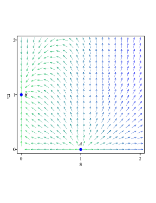
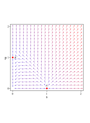
Figure 2: The phase space of the normal branch of DGP inspired $f(R)$ models in which curvature fluid plays the role of a phantom scalar field (left) and the quintessence scalar field (right) in the equivalent scalar-tensor theories. Point $A$ in these two cases is the matter dominated phase and it is a repeller, unstable point. Whereas, point $B$ that represents the de Sitter phase, is an attractor point in the first case and a saddle point in the second case.

To achieve the critical points of this system one should set $s^{\prime}=0$ and $p^{\prime}=0$ . Note that the critical points and their stability depend on the value of $w_{curv}$ . Here we investigate the stability of critical points in two different subspaces of the model parameter space where EoS of the curvature fluid has either a phantom or a quintessence character. In table 1, we see that the current accelerating phase of the universe expansion is unstable if the curvature fluid is considered to be a quintessence scalar field ($-1<w_{curv}$) and stable if it is considered to be a phantom field ($w_{curv}<-1$) in the equivalent scalar-tensor theory. This result is compatible with evolution of the deceleration parameter versus the redshift as has been shown in figure $4$. When $z\rightarrow-1$, the accelerating phase (with $q<0$) is stable for $w_{curv}<-1$. It is necessary to mention that whenever $w_{curv}=-1$, the phase space is 1D (here the curvature fluid plays the role of a cosmological constant, the same as $\Lambda DGP$ model. For more details see Ref. (Chimento et al., 2006)). Figure 2 shows the phase space trajectories of the model.

4.2 $F(R,\varphi)$-DGP model

Now we extend the previous model to an even more general case that the modified induced gravity is non-minimally coupled to a canonical scalar field on the brane. This extension allows us to see the role played by the non-minimal coupling of gravity and scalar degrees of freedom in the cosmological dynamics on the brane. We consider a general coupling between gravity and scalar degrees of freedom on the brane (see for instance Nozari, 2008a; Atazadeh et al, 2008; Saavedra & Vasquez, 2009; Nozari, 2008b; Faraoni, 2000; Nozari, 2007a; Barenboim & Lykken, 2008; Bamba et al., 2009). In fact, inclusion of this field brings the theory to realize a smooth crossing of the phantom divide line in a fascinating manner .

The action of this general model is given as follows (Nozari, 2009b)

$$S=\frac{M_{5}^{3}}{2}\int d^{5}x\sqrt{-g}{\cal{R}}+\int d^{4}x\sqrt{-q}\Big{(}\frac{m_{p}^{2}}{2}F(R,\phi)-\frac{1}{2}q^{\mu\nu}\nabla_{\mu}\phi\nabla_{\nu}\phi-V(\phi)+M_{5}^{3}\overline{K}+{\cal{L}}_{m}\Big{)},$$ (47)

where the first term shows the usual Einstein-Hilbert action in the 5D bulk. The second term on the right hand side is a generalization of the Einstein-Hilbert action induced on the brane. This is an extension of the scalar-tensor theories in one side and a generalization of $f(R)$-gravity on the other side. $\overline{K}$ is the trace of the mean extrinsic curvature on the brane in the higher dimensional bulk, corresponding to the York-Gibbons-Hawking boundary term. We call this model as $F(R,\phi)$-DGP scenario. Note that from the above action, the crossover scale takes the following form (Nozari, 2009a)

$$l_{F}=\frac{m_{p}^{2}}{2M_{5}^{3}}F^{\prime}(R,\varphi)=r_{c}\,\,F^{\prime}(R,\varphi)\,,$$ (48)

where as usual $r_{c}=\frac{m_{p}^{2}}{2M_{5}^{3}}$ , and a prime denotes a differentiation with respect to $R$. Since DGP scenario accounts for embedding of the FRW cosmology at any distance scale (Nozari, 2007b), we start with the following line-element

$$ds^{2}=q_{\mu\nu}dx^{\mu}dx^{\nu}+b^{2}(y,t)dy^{2}=-n^{2}(y,t)dt^{2}+a^{2}(y,t)\gamma_{ij}dx^{i}dx^{j}+b^{2}(y,t)dy^{2}\,,$$ (49)

where $\gamma_{ij}$ is a maximally symmetric $3$-dimensional metric defined as $\gamma_{ij}=\delta_{ij}+k\frac{x_{i}x_{j}}{1-kr^{2}}$. Also $k=-1,0,1$ parameterizes the spatial curvature and $r^{2}=x_{i}x^{i}$. We choose the gauge $b^{2}(y,t)=1$ in the normal Gaussian coordinates. The cosmological dynamics on the brane in this model can be described by the following Friedmann equation (see Nozari, 2008a; Atazadeh et al, 2008; Saavedra & Vasquez, 2009; Nozari, 2009a)

$$H^{2}+\frac{k}{a^{2}}=\frac{1}{3m_{p}^{2}F^{\prime}(R,\varphi)}\Bigg{[}\rho^{tot}+\varrho\Big{(}1+\epsilon\sqrt{1+\frac{2}{\varrho}\Big{[}\rho^{tot}-\frac{m_{p}^{2}F^{\prime}(R,\varphi)}{a^{4}}{\cal{E}}_{0}\Big{]}}\Big{)}\Bigg{]}$$ (50)

where $\epsilon=\pm 1$ shows two different embedding of the brane in the bulk,  $\varrho\equiv\frac{6M_{5}^{6}}{m_{p}^{2}F^{\prime}(R,\phi)}$  and  ${\cal{E}}_{0}=3\Big{(}\frac{\dot{a}^{2}}{n^{2}}-a^{\prime 2}+k\Big{)}a^{2}$  is a constant with respect to $y$ ( with $a^{\prime}\equiv\frac{da}{dy}$), see (Dick, 2001) for more detailed discussion on the constancy of this quantity. Total energy density and pressure are defined as  $\rho^{(tot)}=\rho_{m}+\rho_{\phi}+\rho^{(curv)}+\rho_{\Lambda}$  and   $p^{(tot)}=p_{m}+p_{\phi}+p^{(curv)}+p_{\Lambda}$  respectively. The ordinary matter on the brane has a perfect fluid form with energy density $\rho_{m}$ and pressure $p_{m}$, while the energy density and pressure corresponding to non-minimally coupled quintessence scalar field and also those related to curvature fluid are given respectively as follows

$$\rho_{\varphi}=\bigg{[}\frac{1}{2}\dot{\phi}^{2}+n^{2}V(\phi)-6\frac{dF}{d\phi}H\dot{\phi}\bigg{]}_{y=0},$$ (51)

$$p_{\phi}=\bigg{[}\frac{1}{2n^{2}}\dot{\phi}^{2}-V(\phi)+\frac{2}{n^{2}}\frac{dF}{d\phi}(\ddot{\phi}-\frac{\dot{n}}{n}\dot{\phi})+4\frac{dF}{d\phi}\frac{H}{n^{2}}\dot{\phi}+\frac{2}{n^{2}}\frac{d^{2}F}{d\phi^{2}}\dot{\phi}^{2}\bigg{]}_{y=0}\,,$$ (52)

$$\rho^{(curv)}=m_{p}^{2}\bigg{(}\frac{1}{2}\bigg{[}F(R,\phi)-RF^{\prime}(R,\phi)\bigg{]}-3\dot{R}HF^{\prime\prime}(R,\phi)\bigg{)}\,,$$ (53)

$$p^{(curv)}=m_{p}^{2}\bigg{(}{2\dot{R}HF^{\prime\prime}(R,\phi)+\ddot{R}F^{\prime\prime}(R,\phi)+\dot{R}^{2}F^{\prime\prime\prime}(R,\phi)-\frac{1}{2}\Big{[}F(R,\phi)-RF^{\prime}(R,\phi)\Big{]}}\bigg{)}.$$ (54)

Also by definition $\rho_{\Lambda}\equiv\frac{\Lambda}{8\pi G}$. Ricci scalar on the brane is given by

$$R=3\frac{k}{a^{2}}+\frac{1}{n^{2}}\bigg{[}6\frac{\ddot{a}}{a}+6\Big{(}\frac{\dot{a}}{a}\Big{)}^{2}-6\frac{\dot{a}}{a}\frac{\dot{n}}{n}\bigg{]}.$$

We set $n(0,t)=1$ where $y=0$ is chosen to be the location of the brane. By neglecting the dark radiation term in equation (23), we find

$$H^{2}=\frac{8\pi G}{3}(\rho_{m}+\rho_{\varphi}+\rho^{(curv)})+\frac{\Lambda}{3}+\frac{1}{2l_{F}^{2}}+\epsilon\sqrt{\frac{1}{4l_{F}^{4}}+\frac{1}{2l_{F}^{2}}\Big{[}\frac{8\pi G}{3}(\rho_{m}+\rho_{\varphi}+\rho^{(curv)})+\frac{\Lambda}{3}\Big{]}}\,,$$ (55)

where $G=G_{eff}\equiv\frac{1}{8\pi m_{p}^{2}F^{\prime}(R,\varphi)}$. By adopting the negative sign, we have

$$H^{2}=\frac{8\pi G}{3}(\rho_{m}+\rho_{\varphi}+\rho^{(curv)})+\frac{\Lambda}{3}-\frac{H}{r_{c}F^{\prime}(R,\varphi)}\,.$$ (56)

Comparing this equation with the following Friedmann equation

$$H^{2}=\frac{8\pi G}{3}(\rho_{m}+\rho_{\varphi}+\rho^{(curv)})+\rho_{DE}^{eff}\,,$$ (57)

we are led to conclude that the screening effect on the cosmological constant is modified by $F^{\prime}(R,\varphi)$ as follows

$$\frac{8\pi G}{3}\rho_{DE}^{eff}=\frac{\Lambda}{3}-\frac{H}{r_{c}F^{\prime}(R,\varphi)}\,.$$ (58)

To see how this model works, we consider an explicit form of $F(R,\varphi)$ as $F(R,\varphi)=\frac{1}{2}(1-\xi\phi^{2})[R-(1-n)\zeta^{2}(R/\zeta^{2})^{n}]$ where $\zeta$ is a suitably chosen parameter (see for instance Capozziello, 2003; Sotiriou, 2010; Nojiri & Odintsov, 2003, 2004, 2005, 2006; Nojiri et al., 2007; Nojiri & Odintsov, 2008; Bamba et al., 2008; Carroll et al., 2004; Amendola et al., 2007; Starobinsky, 2007) and (Capozziello et al., 2008, 2010). For a spatially flat FRW geometry, the Ricci scalar is given by $R=6\frac{\ddot{a}}{a}+6(\frac{\dot{a}}{a})^{2}.$ One can investigate variation of the effective dark energy density with respect to parameters $\xi$, $t$ and $n$ to see the status of phantom mimicry in this model. As has been shown in Ref. (Nozari, 2009a), this model accounts for, and modifies the phantom like behavior on the brane. Using the conservation equation $\dot{\rho}_{eff}+3H(1+\omega_{eff})\rho_{eff}=0$, fulfillment of the condition $w_{eff}<-1$  requires the constraint $\frac{\dot{H}}{H}<\frac{\dot{F}^{\prime}(R,\phi)}{F^{\prime}(R,\phi)}$ (Nozari, 2009a). In this situation, this model has the potential to realize the phantom-like behavior and smooth crossing of the phantom divide line by the effective equation of state parameter. Now, in order to compare the $F(R,\varphi)$-DGP model with $\Lambda$CDM and also with other alternative models, we study expansion histories of these models based on the variation of their luminosity distances versus the redshift. The evolution of the cosmic expansion in the normal branch of this F(R,$\varphi$)-DGP setup is given by

$$\frac{H^{2}(z)}{H_{0}^{2}}=\Omega_{m}(1+z)^{3}+\Omega_{\varphi}(1+z)^{3(1+\omega_{\varphi})}+\Omega_{curv}(1+z)^{3(1+\omega_{curv})}+\Omega_{\Lambda}+2\Omega_{r_{c}}$$

$$-2\sqrt{\Omega_{r_{c}}}\sqrt{\Omega_{m}(1+z)^{3}+\Omega_{\varphi}(1+z)^{3(1+\omega_{\varphi})}+\Omega_{curv}(1+z)^{3(1+\omega_{curv})}+\Omega_{\Lambda}+\Omega_{r_{c}}}\,\,.$$ (59)

Note that by definition, $\Omega_{r_{c}}=\frac{1}{4r_{c}^{2}H_{0}^{2}F^{\prime}(R,\varphi)}$ and we use the normalization $F^{\prime}(R,\varphi)|_{(z=0)}\simeq 1$. This model has the disadvantage that it contains more free parameters than $\Lambda$CDM and even $\Lambda$DGP. However, this larger parameter space provides, at least theoretically, more facilities to realize some interesting features. The parameter space of this model can be constraint at $z=0$ so that

$$1=\bigg{(}\sqrt{\Omega_{m}+\Omega_{\varphi}+\Omega_{curv}+\Omega_{\Lambda}+\Omega_{r_{c}}}-\sqrt{\Omega_{r_{c}}}\bigg{)}^{2}.$$ (60)

Since $\Omega_{r_{c}}$  and   $\Omega_{m}+\Omega_{\varphi}+\Omega_{curv}+\Omega_{\Lambda}+\Omega_{r_{c}}$   should be positive, there are two possibilities for constrains on the parameters of this model as follows (Sahni & Shtanov, 2003; Sahni, 2004; Shtanov, 2000; Lue & Starkman, 2004)

$$\Omega_{m}+\Omega_{\varphi}+\Omega_{curv}+\Omega_{\Lambda}-2\sqrt{\Omega_{r_{c}}}=1.$$ (61)

$$\Omega_{m}+\Omega_{\varphi}+\Omega_{curv}+\Omega_{\Lambda}+2\sqrt{\Omega_{r_{c}}}=1.$$ (62)

In our forthcoming analysis, we consider the first one of these constraints. Finally, using equation (13), we compare the luminosity distance - redshift relation of this model with other proposed scenarios. The results are shown in figure $3$. In comparison with $\Lambda$DGP and $f(R)$-DGP, the $F(R,\varphi)$-DGP scenario has the potential to have a better fit with $\Lambda$CDM. The parameters adopted in this model are $\Omega_{m}=0.27$ , $\Omega_{r_{c}}=0.01$ , $\Omega_{\varphi}=0.1$ , $\Omega_{curv}=0.13$ and $\Omega_{\Lambda}=0.7$.

4.3 $F(G,\varphi)$-DGP model

In the $F(G,\varphi)$-DGP setup, the curvature corrections are taken into account via incorporation of the Gauss-Bonnet invariant term in the brane part of the action. The Gauss-Bonnet invariant should be considered essentially in the bulk action. But, if there is a coupling between scalar degrees of freedom on the brane and the mentioned invariant term, then it is necessary to consider its contribution in the field equations on the brane too. This is the main reason for incorporating scalar field $\varphi$ in the $F(G,\varphi)$ setup. We start with the action of this scenario as follows (Nozari et al., 2009; Nojiri et al., 2007; Bamba et al., 2010)

$${\cal{S}}=\frac{M_{5}^{3}}{2}\int d^{5}x\sqrt{-g}{\cal{R}}+\int d^{4}x\sqrt{-q}\bigg{[}\frac{m_{p}^{2}}{2}R+M_{5}^{3}\overline{K}+F(G,\phi)+{\cal{L}}_{m}\bigg{]}.$$ (63)

The Scalar-Gauss-Bonnet term in this action is defined as (Nozari et al., 2009)

$$F(G,\phi)\equiv-\frac{1}{2}\partial_{\mu}\phi\partial^{\mu}\phi-V(\phi)+f(\phi)G(R).$$

By definition, the Gauss-Bonnet invariant $G(R)$ is given by

$$G(R)=R^{2}-4R_{\mu\nu}R^{\mu\nu}+R_{\mu\nu\alpha\beta}R^{\mu\nu\alpha\beta}.$$ (64)

In order to discuss about cosmological dynamics on the brane, one can achieve the generalized Friedmann equation as follows (Nozari et al., 2009)

$$H^{2}+\frac{k}{a^{2}}=\frac{\rho_{m}+\rho^{(GB)}}{3m_{p}^{2}}+\frac{1}{2r_{c}^{2}}+\varepsilon\sqrt{\frac{1}{4r_{c}^{4}}+\frac{1}{r_{c}^{2}}\Big{(}\frac{\rho_{m}+\rho^{GB}}{3m_{p}^{2}}\Big{)}}.$$ (65)

The energy density corresponding to the Gauss-Bonnet term is defined as

$$\rho^{(GB)}\equiv\frac{1}{2}\dot{\phi}^{2}+V(\phi)-24\dot{\phi}f^{\prime}(\phi)H^{3},$$ (66)

and the corresponding pressure is defined as

$$p^{(GB)}=\frac{1}{2}\dot{\phi}^{2}-V(\phi)+8\frac{\partial}{\partial t}\Big{(}H^{2}\dot{f}\Big{)}+16\dot{\phi}f^{\prime}(\phi)H^{3},$$ (67)

where a dot marks differentiation with respect to the cosmic time. One can express the Friedmann equation (65) for the normal branch of this DGP-inspired scenario and for an spatially flat brane in a dimensionless form as follows

$$\frac{H^{2}(z)}{H_{0}^{2}}=\Omega_{m}(1+z)^{3}+\Omega_{GB}(1+z)^{3(1+\omega_{GB})}+2\Omega_{r_{c}}$$

$$-2\sqrt{\Omega_{r_{c}}}\sqrt{\Omega_{m}(1+z)^{3}+\Omega_{GB}(1+z)^{3(1+\omega_{GB})}+\Omega_{r_{c}}}$$ (68)

where by definition $\Omega_{GB}=\frac{8\pi G}{3H_{0}^{2}}\rho_{0}^{(GB)}$. At the red-shift $z=0$, equation (68) can be expressed as

$$1=\bigg{(}\sqrt{\Omega_{m}+\Omega_{GB}+\Omega_{r_{c}}}-\sqrt{\Omega_{r_{c}}}\bigg{)}^{2}.$$ (69)

By choosing the positive sign of the square root, this constrain equation yields

$$\Omega_{m}+\Omega_{GB}-2\sqrt{\Omega_{r_{c}}}=1.$$ (70)

Note that the general relativistic limit can be recovered if we set $\Omega_{r_{c}}=0$ (or $M_{5}=0$). In this case equation (70) implies $\Omega_{m}+\Omega_{GB}=1$. Finally, the luminosity distance-redshift of this model is compared with other proposed alternatives in figure $3$.

5 Some other probes

To have more complete comparison between the proposed models, in this section we study some other features of these models. The current universe is accelerating and this can be realized by investigating the deceleration parameter. The deceleration parameter $q=-\frac{\ddot{a}}{\dot{a}^{2}}a$ can be expressed as

$$q(z)=\frac{H^{\prime}(z)}{H(z)}(1+z)-1\,,$$ (71)

where a prime marks differentiation with respect to $z$. We study variation of $q$ versus the redshift in each of the previously proposed models. For this purpose, we use $H(z)$ as given by equations (9),  (12),  (18),  (59) and (68). Figure $4$ compares the deceleration parameter in each of the proposed scenarios. All of these scenarios explain the late-time cosmic speed-up in their normal DGP branches, but the redshift at which transition to the accelerated phase occurs are different in these scenarios. The $\Lambda$DGP model transits to the accelerated phase at $z\simeq 0.8$ much sooner than other scenarios. The $F(R,\varphi)$-DGP model transits to the accelerated phase at $z\simeq 0.4$ much later than other alternatives. We note however that the exact value of the transit redshift depends on the choice of the parameters in each model. Within the parameters values adopted here, the result are shown in figure $4$. As another important result, we note that late-time acceleration in the $f(R)$-DGP universe is a stable phenomenon since we considered the curvature fluid to be a phantom scalar field. Also the acceleration phase is a transient phenomenon for $F(G,\varphi)$-DGP model if we set $w_{\varphi}>-1$. Our inspection shows that cosmological dynamics in the normal branch of $f(R)$-DGP scenario with a quintessence curvature fluid is very similar to cosmological dynamics in the normal branch of $F(G,\varphi)$-DGP scenario for $w_{GB}>-1$.

The next probe is the age of the universe in each of these scenarios. The age of the universe at a given cosmological red-shift is given as follow

$$t(z)=\int_{z}^{\infty}\frac{dz^{\prime}}{(1+z^{\prime})H(z^{\prime})}\,,$$ (72)

where $H(z)$ is given in each of the proposed scenarios. In figure $5$ the age of the universe is compared in five alternative scenarios. Within the parameter values adopted here, the age of the universe in $f(R)$-DGP is larger than $\Lambda$CDM, but this age in $F(G,\varphi)$-DGP is smaller than $\Lambda$CDM one.

6 Summary

In this paper, observational status of the $\Lambda$CDM , $\Lambda$DGP and some extended phantom-like cosmologies as alternatives for dark energy are studied. We compared these models with each other by comparing variation of their luminosity distances versus the redshift and also the age of the universe in each of these scenarios. The common feature of the mentioned DGP-inspired scenarios is possibility of realization of the phantom-like behavior in their normal DGP branches. In the extended scenarios, we focused on the role played by new ingredients such as the curvature effect, modification of the induced gravity on the brane and even the existence of a quintessence field non-minimally coupled to modified induced gravity on the brane. Since all of our analysis are preformed on the normal DGP branch of each scenario, there is no ghost instabilities in these setups. As an example and to have an intuition about stability of the solutions, we analyzed stability of cosmological phases of $f(R)$-DGP scenario within a dynamical system approach. We have analyzed the phase space of the normal branch of this model where curvature fluid plays the role of a phantom or quintessence scalar field in the equivalent scalar-tensor theory. We have shown that the matter dominated phase of this model is a repeller, unstable point. However, there is a de Sitter phase which is an attractor point if curvature fluid plays the role of a phantom scalar field in the equivalent scalar-tensor theory. For a quintessence field plying the role of the curvature fluid, the de Sitter phase is an unstable, saddle point. Up to the parameters values adopted in this paper, $F(R,\varphi)$-DGP scenario mimics the behavior of the $\Lambda$CDM scenario more than other proposed models. As another important outcome, all of these scenarios explain the late-time cosmic speed-up in their normal DGP branches, but the redshift at which transition to the accelerating phase occurs are different in these scenarios. For instance, the $\Lambda$DGP model transits to the accelerating phase at $z\simeq 0.8$, much sooner than other scenarios. However, the $F(R,\varphi)$-DGP model transits to the accelerated phase at $z\simeq 0.4$, much later than other alternatives. Nevertheless, the exact value of the transit redshift depends on the choice of the parameters in each model. Finally, we compared the age of the universe in each of the proposed scenarios. Within the parameter values adopted in this paper, the age of the universe in the $f(R)$-DGP model is larger than $\Lambda$CDM, but this age in $F(G,\varphi)$-DGP is smaller than $\Lambda$CDM one.

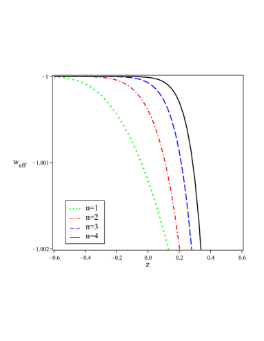
Figure 1: $w_{curv}$ versus the redshift for a DGP-inspired $f(R)$ model. The $f(R)$ is chosen to be the Hu-Sawicki model. The selected free parameters in plotting this figure are chosen to be $\Omega_{m}=0.27$ ,$\Omega_{\Lambda}=0.93$ ,$\Omega_{r_{c}}=0.01$ and $f_{0}^{\prime}(R)-1=10^{-6}$ . As this figure shows, in this class of models the curvature fluid has an effective phantom equation of state with $w_{curv}<-1$ at high redshifts. This effective equation of state parameter approaches the phantom divide line ($w_{curv}=-1$) at a redshift that decreases by decreasing the value of $n$.

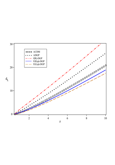
Figure 3: Luminosity distance versus the red-shift for five alternative scenarios proposed in this paper. In this figure we have set $(\Omega_{m},\Omega_{r_{c}})=(0.27,10^{-2})$ for all of the models and $(\Omega_{\varphi},\Omega_{\Lambda},\Omega_{curv})=(0.1,0.7,0.13)$ for the $F(R,\varphi)$-DGP setup, $\Omega_{\Lambda}=0.93$ for the $\Lambda$DGP, $\Omega_{curv}=0.93$ for the $f(R)$-DGP setup and $\Omega_{GB}=0.93$ . We calculated these quantities using the constraint equations attributed to each model. Up to the parameters values adopted here, $F(R,\varphi)$-DGP scenario is closer to the $\Lambda$CDM than other proposed models. We note however that this result depends strongly on the adapted parameters values.

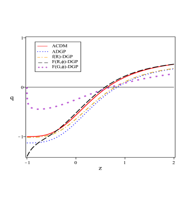
Figure 4: The deceleration parameter $q(z)$ versus the red-shift for five alternative scenarios discussed in this paper. The model parameters are the same as adopted in figure $3$ and $w_{curv}$ here is adopted quintessence like in the left and phantom like in the right. Note that current acceleration in the $f(R)$-DGP universe in which curvature fluid play role of a quintessence is a transient and unstable phenomenon but if it act as a phantom field, it result in a stable accelerated phase for the universe.

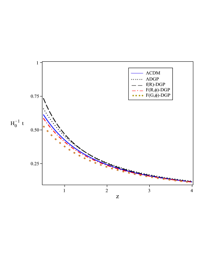
Figure 5: The age of the universe (in units of the inverse Hubble parameter) versus the red-shift for five alternative scenarios discussed in this paper. The model parameters are the same as adopted in figure 3. With proposed parameter values, the $f(R)$-DGP model has the largest and the $F(G,\varphi)$-DGP has the smallest age.

Table 1: Eigenvalues and the stability properties of the critical points.

points	$(s,p)$	eigenvalues	for $w_{curv}<-1$	for $(-1<w_{curv}<0)$
$A$	$(1,0)$	$(-\frac{3w_{curv}}{2},\frac{3}{2})$	unstable	unstable
$B$	$(0,1)$	$(\frac{3w_{curv}}{2},\frac{3(1+w_{curv})}{2})$	stable	unstable

References

- Perlmutter (1999) Perlmutter, S. et al 1999, AJ, 517, 565
- Riess (1998) Riess, A. G. 1998, AJ, 116, 1006
- Astier et al. (2006) Astier, P. et al., 2006, å, 447, 31
- Wood-Vasey et al. (2007) Wood-Vasey, W. M. et al., 2007, AJ, 666, 694
- Miller et al. (1999) Miller, A. D. et al., 1999, AJL, 524, L1
- Hanany (2000) Hanany, S. 2000, AJL, 545, L5
- Spergel et al. (2003) Spergel, D. N. et al., 2003, AJS, 148, 175
- Colless et al. (2001) Colless, M. et al., 2001, MNRAS, 328, 1039
- Tegmark et al. (2004) Tegmark, M et al., 2004, Phys. Rev. D, 69, 103501
- Cole et al. (2005) Cole, S. et al., 2005, MNRAS, 362, 505
- Springel et al. (2006) Springel, V., Frank, C. S., & White, S. M. D. 2006, Nature (London), 440, 1137
- Sahni & Starobinsky (2000) Sahni, V. & Starobinsky, A. A. 2000, Int. J. Mod. Phys. D, 9, 373
- Padmanabhan (2003) Padmanabhan, T. 2003, Phys. Rep, 380, 235
- Copeland et al. (2006) Copeland, E. J., Sami, M., & Tsujikawa, S. 2006, 15, 1753
- Weinberg (1989) Weinberg, S. 1989, Rev. Mod. Phys., 61, 1
- Carroll (2001) Carroll, S. M. 2001, Living Rev. Relativity, 4, 1
- Caldwell et al. (1999) Caldwell, R. R., Dave, R., & Steinhardt, P. 1999, Phys. Rev. D, 59, 504
- Ratra & Peebles (1988) Ratra, B., & Peebles, P. J. E. 1988, Phys. Rev. D, 37, 3406
- Sahni & Wang (2000) Sahni, V., & Wang, L. 2000, Phys. Rev. D, 62, 103517
- Saini et al. (2000) Saini, T. D., Raychaudhury, S., Sahni, V., & Starobinsky, A. A. 2000, Phys. Rev. Lett., 85, 1162
- Brax & Martin (2000) Brax, P., Martin, J. 2000, Phys. Rev. D, 61, 103502
- Barreiro et al. (2000) Barreiro, T., Copeland, E. J., & Nunes, N. J. 2000, Phys. Rev. D, 61, 127301
- Sahni et al. (2002) Sahni, V., Sami, M., & Souradeep, T. 2002, Phys. Rev. D, 65, 023518
- Sami et al. (2003) Sami, M., Dadhich, N., & Shiromizu, T. 2003, Phys. Lett. B, 568, 118
- Sami & Padmanabhan (2003) Sami, M., & Padmanabhan, T. 2003, Phys. Rev. D, 67, 083509
- Caldwell (2002) Caldwell, R. R. 2002, Phys. Lett. B, 545, 23
- Tsujikawa & Sami (2004) Tsujikawa, S., & Sami, M. 2004, Phys. Lett. B, 603, 113
- Caldwell & Linder (2005) Caldwell, R. R., & Linder, E. V. 2005, Phys. Rev. Lett., 95, 141301
- Cai et al. (2010) Cai, Y. -F., Saridakis, E. N., Setare, M. R., & Xia, J. -Q. 2010, Phys. Reports, 493, 1-60
- Moyassari & Setare (2009) Moyassari, P. & Setare, M. R., 2009, Phys. Lett. B, 674, 237
- Kamenshchik et al. (2001) Kamenshchik, A., Moschella, U., & Pasquier, V. 2001, Phys. Lett. B, 511, 265
- Dev et al. (2003) Dev, A., Alcaniz, J. S., & Jain, D. 2001, Phys. Rev. D, 67, 023515 37
- Amendola et al. (2003) Amendola, L., Finelli, F., Burigana, C., & Carturan, D. 2003, J. Cosmology Astropart. Phys, 0307, 005
- Bertolami et al. (2004) Bertolami, O., Sen, A. A., & Silva, P. T. 2004, MNRAS, 353, 329
- Biesiada et al. (2005) Biesiada, M., Godlowski, W., & Szydlowski, M. 2005, AJ, 622, 28
- Zhang et al. (2006a) Zhang, X., Wu, F. -Q., & Zhang, J. 2006a, J. Cosmology Astropart. Phys, 0601, 003
- Zhang & Zhu (2006b) Zhang, H., & Zhu, Z. -H. 2006b, Phys. Rev. D, 73, 043518
- Zhang et al. (2009) Zhang, H., Zhu, Z. -H., & Yang, L. 2009, Mod. Phys. Lett. A, 24, 541
- Heydari-Fard & Sepangi (2008) Heydari-Fard, M., & Sepangi, H. R. 2008, Phys. Rev. D, 78, 064007
- Roos (2007) Roos, M. 2007, [arXiv:0704.0882]
- Bouhmadi-López & Lazkoz (2007) Bouhmadi-López, M., & Lazkoz, R. 2007, Phys. Lett. B, 654, 51
- Roos (2008a) Roos, M. 2008a, [arXiv:0804.3297]
- Roos (2008b) Roos, M. 2008b, Phys. Lett. B, 666, 420
- Setare (2009) Setare, M. R. 2009, Int. J. Mod. Phys. D, 18, 419
- Capozziello (2003) Capozziello, S., V. F., Cardone, Carloni, S., & Troisi, A. 2003, Int. J. Mod. Phys. D, 12, 1969
- Sotiriou (2010) Sotiriou, T. P., & Faraoni, V. 2010, [ arXiv:/0805.1726]
- Nojiri & Odintsov (2007) Nojiri, S., & Odintsov, S. D. 2007, Int. J. Geom. Meth. Mod. Phys., 4, 115
- Nojiri & Odintsov (2004) Nojiri, S., & Odintsov, S. D. 2004, Gen. Relat. Gravit., 36, 1765
- Nojiri & Odintsov (2003) Nojiri, S., & Odintsov, S. D. 2003, Phys. Rev. D, 68, 123512
- Nojiri & Odintsov (2005) Nojiri, S., & Odintsov, S. D. 2005, Class. Quantum Grav., 22, L35
- Nojiri & Odintsov (2006) Nojiri, S., & Odintsov, S. D. 2006, Phys. Rev. D, 74, 086009
- Nojiri & Odintsov (2008) Nojiri, S., & Odintsov, S. D. 2008, Phys. Rev. D, 78, 046006
- Bamba et al. (2008) Bamba, K., Nojiri, S., & Odintsov, S. D. 2008, J. Cosmology Astropart. Phys, 0810, 045
- Carroll et al. (2004) Carroll, S. M., Duvvuri, V., Trodden, M., & Turner, M. S. 2004, Phys. Rev. D, 70, 043528
- Amendola et al. (2007) Amendola, L., Polarski, D., & Tsujikawa, S. 2007, Phys. Rev. Lett., 98, 131302
- Starobinsky (2007) Starobinsky, A. 2007, JTEP, 86, 157
- Nozari (2008a) Nozari, K., & Pourghassemi, M. 2008a, J. Cosmology Astropart. Phys, 10, 044
- Atazadeh et al (2008) Atazadeh, K., Farhoudi, M., & Sepangi, H. R. 2008, Phys. Lett. B, 660, 275
- Saavedra & Vasquez (2009) Saavedra, J., & Vasquez, Y. 2009, J. Cosmology Astropart. Phys, 04, 013
- Setare (2008) Setare, M. R. 2008, Int. J. Mod. Phys. D, 17, 2219
- Dvali et al. (2000a) Dvali, G. R., Gabadadze, G., & Porrati, M. 2000a, Phys. Lett. B, 484, 112
- Deffayet (2001) Deffayet, C. 2001, Phys. Lett. B, 502, 199
- Lue (2006) Lue, A. 2006, Phys. Rept., 423, 48
- Dvali et al. (2000b) Dvali, G. R., Gabadadze, G., & Porrati, M. 2000b, Phys. Lett. B, 485, 208
- Dvali & Gabadadze (2001) Dvali, G. R., & Gabadadze, G. 2001, Phys. Rev. D, 63, 065007
- Dvali et al. (2002) Dvali, G. R., Gabadadze, G., Kolanovi, M., & Nitti, F. 2002, Phys. Rev. D, 65, 024031
- Melchiorri et al. (2003) Melchiorri, A., Mersini, L., Odman, C. G., & Trodden, M. 2003, Phys. Rev. D, 68, 043509
- Riess et al. (2004) Riess, A. G. et al. 2004, AJ, 607, 665
- Komatsu et al. (2009) Komatsu, E. et al. [WMAP Collaboration] 2009, AJS, 180, 330
- Sahni & Shtanov (2003) Sahni, V., & Shtanov, Y. 2003, J. Cosmology Astropart. Phys, 0311, 014 0005193
- Sahni et al. (2005) Sahni, V., Shtanov, Y., & Viznyuk, A. 2005, J. Cosmology Astropart. Phys, 0512, 005
- Sahni (2004) Sahni, V. 2004, [arXiv:astro-ph/0502032]
- Shtanov (2000) Shtanov, Y. V. 2000, [arXiv:hep-th/0005193]
- Lue & Starkman (2004) Lue, A., & Starkman, G. D. 2004, Phys. Rev. D, 70, 101501
- Collins & Holdom (2000) Collins, H., & Holdom, B. 2000, Phys. Rev. D, 62, 105009
- Lazkoz et al. (2006) Lazkoz, R., Maartens, R., & Majerotto, E. 2006, Phys. Rev. D, 74, 083510
- Maartens & Majerotto (2006) Maartens, R. & Majerotto, E. 2006, Phys. Rev. D, 74, 023004
- Lazkoz & Majerotto (2007) Lazkoz, R. & Majerotto, E. 2006, J. Cosmology Astropart. Phys, 07, 015
- Alam & Sahni (2006) Alam, U. & Sahni, V. 2006, Phys. Rev. D, 73, 084024
- Sollerman et al. (2009) Sollerman, J. et al. 2009, AJ, 703, 1374
- Nozari (2009a) Nozari, K., & Kiani, F. 2009a, J. Cosmology Astropart. Phys, 07, 010
- Bouhmadi-Lopez (2009) Bouhmadi-Lopez, M. 2009, J. Cosmology Astropart. Phys, 0911, 011
- Nozari (2009b) Nozari, K., & Rashidi, N. 2009b, J. Cosmology Astropart. Phys, 0909, 014
- Nozari (2009c) Nozari, K., & Azizi, T. 2009c, Phys. Lett. B, 680, 205
- Nozari (2009d) Nozari, K., & Aliopur, N. 2009d, Europhys. Lett., 87, 69001
- Atazadeh & Sepangi (2006) Atazadeh, K., & Sepangi, H. R. 2006, Phys. Lett. B, 643, 76
- Atazadeh & Sepangi (2007) Atazadeh, K., & Sepangi, H. R. 2007, J. Cosmology Astropart. Phys, 0709, 020
- Atazadeh & Sepangi (2009) Atazadeh, K., & Sepangi, H. R. 2009, J. Cosmology Astropart. Phys, 01, 006
- Hu & Sawicki (2007) Hu, W. & Sawicki, I. 2007, Phys. Rev. D, 76, 064004
- Martinelli et al. (2009) Martinelli, M., Melchiorri, A., & Amendola, L. 2009, Phys. Rev. D, 79, 123516
- Cai et al. (2007) Cai, Y. -Fu., Qiu, T., Piao, Y. -S., & Zhang, X. 2007, JHEP, 071, 0710
- Faraoni (2000) Faraoni V. 2000, Phys. Rev. D, 62, 023504
- Nozari (2007a) Nozari, K. 2007a, J. Cosmology Astropart. Phys, 0709, 003
- Nozari (2008b) Nozari, K., & Fazlpour, B. 2008b, J. Cosmology Astropart. Phys, 0806, 032
- Barenboim & Lykken (2008) Barenboim, G., & Lykken, J. 2008, J. Cosmology Astropart. Phys, 0803, 017
- Bamba et al. (2009) Bamba, K., Geng, C. -Q., Nojiri, S., & Odintsov, S. D. 2009, Phys. Rev. D, 79, 083014
- Chimento et al. (2006) Chimento, L. P., Lazkoz, R., Maartens, R., & Quiros, I. 2006, J. Cosmology Astropart. Phys, 0609, 004
- Nozari (2007b) Nozari, K. 2007b, Phys. Lett. B, 652, 159
- Dick (2001) Dick, R. 2001, Class. Quant. Grav., 18, R1
- Capozziello et al. (2008) Capozziello, S., Cardone, V. F., & Salzano, V. 2008, Phys. Rev. D, 78, 063504
- Capozziello et al. (2010) Capozziello, S., Laurentis, M., & Faraoni, V. 2010, [ arXiv:0909.4672]
- Nozari et al. (2009) Nozari, K., Azizi, T., & Setare, M. R. 2009, J. Cosmology Astropart. Phys, 010, 022
- Nojiri et al. (2007) Nojiri, S., Odintsov, S. D., & Tretyakov, P. V. 2007, Phys. Lett. B, 651, 224
- Bamba et al. (2010) Bamba, K., Odintsov, S. D., Sebastiani, L., & Zerbini, S. 2010, [arXiv:0911.4390]