Closed planar curves without inflections

Abstract.

We define a computable topological invariant $\mu(\gamma)$ for generic closed planar regular curves $\gamma$, which gives an effective lower bound for the number of inflection points on a given generic closed planar curve. Using it, we classify the topological types of ‘locally convex curves’ (i.e. closed planar regular curves without inflections) whose numbers of crossings are less than or equal to five. Moreover, we discuss the relationship between the number of double tangents and the invariant $\mu(\gamma)$ on a given $\gamma$.

1. Introduction.

In this paper, curves are always assumed to be regular (i.e. immersed). The well-known Fabricius-Bjerre [3] theorem asserts (see also [5]) that

(0.1) $$d_{1}(\gamma)-d_{2}(\gamma)=\#_{\gamma}+\frac{i_{\gamma}}{2}$$

holds for closed curves $\gamma$ satisfying suitable genericity assumptions, where $d_{1}(\gamma)$ (resp. $d_{2}(\gamma)$) is the number of double tangents of same side (resp. opposite side) and $\#_{\gamma}$ and $i_{\gamma}$ are the number of crossings and the number of inflections on $\gamma$, respectively.

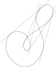
Figure 1. A curve with $\#_{\gamma}=2$, $i_{\gamma}=2$, $d_{1}=4$ and $d_{2}=1$.

However, for arbitrarily given non-negative integers $d_{1},d_{2},n$ and $i$ satisfying $d_{1}-d_{2}=n+i/2$, there might not exist a corresponding curve, in general. As an affirmative answer to the Halpern conjecture in [6], the second author [8] proved the inequality

(0.2) $$d_{1}(\gamma)+d_{2}(\gamma)\leq\#_{\gamma}(2\#_{\gamma}-1)$$

for closed curves without inflections (see Remark 3.4). It is then natural to expect that there might be further obstructions for the topology of closed planar curves without inflections. In this paper, we define a computable topological invariant $\mu(\gamma)$ for closed planar curves. By applying the Gauss-Bonnet formula, we show the inequality $i_{\gamma}\geq\mu(\gamma)$, which is sharp at least for closed curves satisfying $\#_{\gamma}\leq 4$. In fact, for such $\gamma$, there exists a closed curve $\sigma$ which has the same topological type as $\gamma$ such that $i_{\sigma}=\mu(\sigma)$. As an application, we classify the topological types of closed planar curves satisfying $i_{\gamma}=0$ and $\#_{\gamma}\leq 5$. Moreover, we discuss the relationship between the number of double tangents of the curve and the invariant $I(\gamma)$ on a given $\gamma$.

1. Preliminaries and main results

We denote by $\bm{R}^{2}$ the affine plane, and by $S^{2}$ the unit sphere in $\bm{R}^{3}$. A closed curve $\gamma$ in $\bm{R}^{2}$ or $S^{2}$ is called generic if

1. all crossings are transversal, and

2. the zeroes of curvature are nondegenerate.

By stereographic projection, we can recognize $S^{2}=\bm{R}^{2}\cup\{\infty\}$. Two generic closed curves $\gamma_{1}$ and $\gamma_{2}$ in $\bm{R}^{2}$ (in $S^{2}$) are called geotopic, or said to have the same topological type, in $\bm{R}^{2}$ (resp. in $S^{2}$) if there is an orientation preserving diffeomorphism $\varphi$ of $\bm{R}^{2}$ (resp. on $S^{2}$) such that $\operatorname{Im}\gamma_{2}=\varphi(\operatorname{Im}\gamma_{1}).$ This induces an equivalence relation on the set of closed curves. We denote equivalence classes by $\langle\gamma_{1}\rangle$ (resp. $[\gamma_{1}]$). We fix a closed regular curve $\gamma:S^{1}\to\bm{R}^{2}$. A point $c\in S^{1}$ is called an inflection point of $\gamma$ if $\operatorname{det}(\dot{\gamma}(t),\ddot{\gamma}(t))$ vanishes at $t=c$. We denote by $i_{\gamma}$ the number of inflection points on $\gamma$. A closed curve $\gamma:[0,1]\to\bm{R}^{2}$ is called locally convex if $i_{\gamma}=0$. Whitney [13] proved that any two closed curves are regularly homotopic if and only if their rotation indices coincide. So then one can ask if this regular homotopy preserves the locally convexity when the given two curves are both locally convex. In fact, one can easily prove this by a modification of Whitney’s argument, which has been pointed out in [9, p35, Exercise 11]. For the sake of the readers’ convenience we shall outline the proof:

Proposition 1.1.

Let $\gamma_{1}$ and $\gamma_{2}$ be two locally convex closed regular curves. Suppose that $\gamma_{1}$ has the same rotation index as $\gamma_{2}$. Then there exists a family of closed curves $\{\Gamma_{\varepsilon}\}_{\varepsilon\in[0,1]}$ such that

1. $\Gamma_{0}=\gamma_{1}$ and $\Gamma_{1}=\gamma_{2}$,

2. each $\Gamma_{\varepsilon}$ $(\varepsilon\in[0,1])$ is a locally convex closed regular curve.

Proof.

Suppose that the curves $\gamma_{j}$ $(j=1,2)$ are both positively curved and have the same rotation indices, equal to $m$. We change, if necessary, the parametrizations of $\gamma_{j}$ so that the tangent vectors $\dot{\gamma}_{j}(t)$ are positive scalar multiples of ${\begin{pmatrix}\cos t\\ \sin t\end{pmatrix}}$. Define a homotopy $\Gamma_{\varepsilon}$ between $\gamma_{1}$ and $\gamma_{2}$ by

$$\Gamma_{\varepsilon}(t)=(1-\varepsilon)\gamma_{1}(t)+\varepsilon\gamma_{2}(t).$$

It is easy to verify that $\{\Gamma_{\varepsilon}\}_{\varepsilon\in[0,1]}$ satisfies the required conditions (1) and (2). ∎

For a given generic closed curve $\gamma$, we set

(1.1) $$I(\gamma):=\min_{\sigma\in\langle\gamma\rangle}i_{\sigma}.$$

Since $i_{\gamma}$ is an even number, so is $I(\gamma)$. Inflection points on curves in $\bm{R}^{2}$ correspond to singular points on their Gauss maps. So it is natural to ask about the existence of topological restrictions on closed curves without inflections, in other words, we are interested in the topological type of closed curves $\gamma$ satisfying $I(\gamma)=0$.

There are explicit combinatorial procedures for determining generic closed spherical curves with a given number of crossings, as in Carter [4] and Cairns and Elton [2] (see also Arnold [1]). We denote by $\#_{\gamma}$ the number of crossings for a given generic closed curve. In this paper, we use the table of closed spherical curves with $\#_{\gamma}\leq 5$ given in the appendix of [7].

For example, the table of closed spherical curves with $\#_{\gamma}\leq 2$ is given in Figure 2, where $1_{2}$ (resp. $2_{2}$) means that the corresponding curve has 2-crossings and appears in the table of curves in [7] with $\#_{\gamma}=2$ primary (resp. secondary).

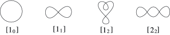
Figure 2. Spherical closed curves with $\#_{\gamma}\leq 2$.

Moving the position of $\infty$ via motions in $S^{2}=\bm{R}^{2}\cup\{\infty\}$, we get the table of closed planar curves with $\#_{\gamma}\leq 2$ as in Figure 3. For example $1_{1}$ and $1_{1}^{b}$ (resp. $2_{2}$, $2_{2}^{b}$ and $2_{2}^{c}$) are equivalent to $[1_{1}]$ (resp. $[2_{2}]$) as spherical curves. Here, only the curves of type $1_{1}$ and $2_{2}$ can be drawn with no inflections. Similarly, using the table of spherical curves with $\#_{\gamma}\leq 5$ given in [7], we prove the following theorem. The authors do not know of any reference for such a classification of generic locally convex curves.

Figure 3. Planar closed curves with $\#_{\gamma}\leq 2$.

Theorem 1.2.

For a given generic closed regular curve $\gamma$ in $\bm{R}^{2}$, the inequality

(1.2) $$I(\gamma)\geq\mu(\gamma)$$

holds. Moreover, $I(\gamma)=0$ if and only if $\mu(\gamma)=0$ under the assumption that $\#_{\gamma}\leq 5$.

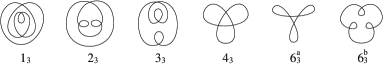
Figure 14. Curves with $I_{\gamma}=0$ and $\#_{\gamma}=3$ (6 curves in total).

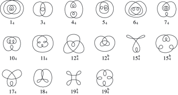
Figure 16. Curves with $I(\gamma)=0$ and $\#_{\gamma}\leq 4$ (16 curves in total).

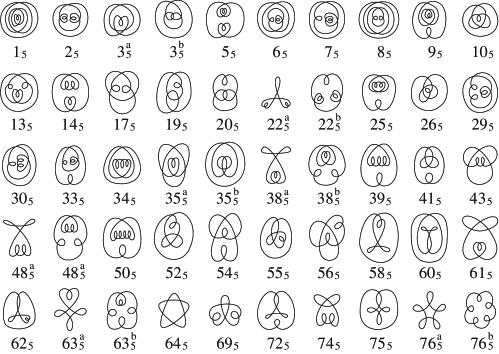
Figure 17. Curves with $I(\gamma)=0$ and $\#_{\gamma}=5$ (50 curves in total).

In particular, the number of equivalence classes of closed locally convex curves with $\#_{\gamma}\leq 5$ is $76$ (see Figure 3 and Figures 14, 16 and 17 in Section 3). For example, in Figure 3 the curves of type $1_{0},1_{1},1_{2},2_{2}$ satisfy $I(\gamma)=0$, and the remaining $1_{1}^{b},1_{2}^{b},2_{2}^{b},2_{2}^{c}$ satisfy $I(\gamma)=2$. In Figure 14, the curve of type $6_{3}^{a}$ is of the same topological type as $6_{3}^{b}$ as a spherical curve, which is obtained from the 6th curve in the table of curves with $\#_{\gamma}=2$ in the appendix of [7].

Corollary 1.3.

A generic closed curve $\gamma$ with $\#_{\gamma}\leq 4$ satisfies $I(\gamma)=\mu(\gamma)\leq 2$, unless the topological type of $\gamma$ is as in Figure 4.

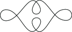
Figure 4. A curve with $\#_{\gamma}=4$ and $I(\gamma)=\mu(\gamma)=4$.

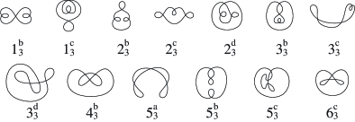
Figure 15. Curves with $I(\gamma)>0$ and $\#_{\gamma}\leq 3$ (13 curves in total).

A table of closed curves $\gamma$ with $i_{\gamma}=\mu(\gamma)$ for $\#_{\gamma}\leq 3$ is given in Figures 3, 14 and 15. For example, in Figure 15, the curves of type $6_{3}^{c}$ consideres as spherical curves are of the same topological type as the curves of type $6_{3}^{a}$ or $6_{3}^{b}$ in Figure 14.

2. Definition of the invariant $\mu(\gamma)$

We fix a generic closed curve $\gamma:S^{1}\to\bm{R}^{2}$. We set $\#_{\gamma}=m$. We may suppose that $\gamma(0)=\gamma(1)$ is one of the crossings of $\gamma$. Let

$$0=c_{1}<\cdots<c_{2m}(<1)$$

be the inverse image of the crossings of $\gamma$, which consists of $2m$ points in $S^{1}=\bm{R}/\bm{Z}$. We set

$$S^{1}_{\gamma}:=S^{1}\setminus\{c_{1},...,c_{2m}\}.$$

To introduce the invariant $\mu(\gamma)$, we define special subsets on the curves called ‘$n$-gons’:

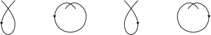
Figure 5. Shells.

Definition 2.1.

Let $n(\geq 3)$ be an integer. A disjoint union of $n$ proper closed intervals

$$J:=[a_{1},b_{1}]\cup\cdots\cup[a_{n},b_{n}]$$

on $S^{1}$ is called an $n$-gon if $a_{1},b_{1},\cdots,a_{n},b_{n}\in\{c_{1},...c_{2m}\}$ and the image $\gamma(J)$ is a piecewise smooth simple closed curve in $\bm{R}^{2}$. The simply connected domain bounded by $\gamma(J)$ is called the interior domain of the $n$-gon. An $n$-gon is called admissible if at most two of the $n$ interior angles of $D$ are less than $\pi$.

We denote by $\mathcal{G}_{n}(\gamma)$ the set of all admissible $n$-gons, and set

$$\mathcal{G}(\gamma):=\bigcup_{n=1}^{\infty}\mathcal{G}_{n}(\gamma).$$

Each element of $\mathcal{G}(\gamma)$ is called an admissible polygon. A $1$-gon is called a shell (cf. Figure 5). A $2$-gon is called a leaf (cf. Figure 6) and a $3$-gon is called a triangle (cf. Figure 7). All shells and all leaves are admissible. However, a triangle whose interior angles are all acute is not admissible.

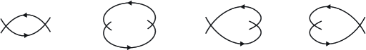
Figure 6. Leaves.

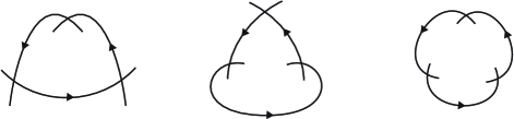
Figure 7. Admissible triangles.

We fix an admissible $n$-gon $J:=[a_{1},b_{1}]\cup\cdots\cup[a_{n},b_{n}].$ Then $\gamma(J)$ is a piecewise smooth simple closed curve in $\bm{R}^{2}$. We give an orientation of $\gamma(J)$ so that the interior domain of $\gamma(J)$ is on the left hand side of $\gamma(J)$. This orientation induces an orientation on $[a_{i},b_{i}]$ for each $i=1,...,n$. We call $[a_{i},b_{i}]$ a positive interval (resp. negative interval) if the orientation of the interval $[a_{i},b_{i}]$ coincides with (resp. does not coincide with) the orientation of $\gamma$.

Let $t$ be a point on $J\setminus\{a_{1},b_{1},...,a_{n},b_{n}\}=\bigcup_{i=1}^{n}(a_{i},b_{i})$. Then $t$ belongs to an open interval $(a_{i},b_{i})$ for some $i=1,...,n$. Then we set

$$\varepsilon_{J}(t):=\begin{cases}1&\mbox{if $[a_{i},b_{i}]$ is positive},\\ -1&\mbox{if $[a_{i},b_{i}]$ is negative}.\end{cases}$$

Definition 2.2.

An admissible $n$-gon is called positive (resp. negative) if $\varepsilon_{J}(t)>0$ (resp. $\varepsilon_{J}(t)<0$) holds for each $t\in J\setminus\{a_{1},b_{1},...,a_{n},b_{n}\}$.

The notions of positivity and negativity of shells were used in [12] and [7] differently from here. The following assertion is the key to proving the inequality (1.2):

Lemma 2.3.

Let $J:=[a_{1},b_{1}]\cup\cdots\cup[a_{n},b_{n}]$ be an admissible $n$-gon. Then there exists an interval $[a_{i},b_{i}]$ ($1\leq i\leq n$) and a point $c\in(a_{i},b_{i})$ such that $\operatorname{sgn}(\kappa_{\gamma}(c))=\varepsilon_{J}(c)$, where $\kappa_{\gamma}(t):={\operatorname{det}(\dot{\gamma}(t),\ddot{\gamma}(t))}/{|\dot{\gamma}|^{3}}$ is the curvature of $\gamma$ and $\operatorname{sgn}(\kappa_{\gamma}(c))$ is the sign of the real number $\kappa_{\gamma}(c)$.

Proof.

Let $A_{1},A_{2},\cdots,A_{n}$ be the interior angles of the interior domain of $J$, and set $\Gamma=\gamma(J)$, which we regard as an oriented piecewise smooth simple closed curve with counterclockwise orientation. In this proof, $\bm{R}^{2}$ is considered as the Euclidean plane, and we take the arclength parameter $s$ of $\Gamma$. Let $s=s_{1},...,s_{n}$ be the points where $d\Gamma/ds$ is discontinuous. We denote by $\kappa_{\Gamma}(s)$ ($s\neq s_{1},...,s_{n}$) the curvature of the curve $\Gamma$. Then, the Gauss-Bonnet formula yields that

$$\int_{J}\kappa_{\Gamma}(s)ds=-(n-2)\pi+\sum_{i=1}^{n}A_{i}.$$

Since $J$ is admissible, we may assume that $A_{1},...,A_{n-2}\geq\pi$, and so $\int_{J}\kappa_{\Gamma}(s)ds>0$. Then there exist an index $i$ $(1\leq i\leq n)$ and $c\in[a_{i},b_{i}]$ such that $\kappa_{\Gamma}(c)>0.$ We denote by $\kappa_{\gamma}(s)$ the Gaussian curvature of $\gamma$ at $\Gamma(s)$. Then we have that

$$0<\kappa_{\Gamma}(c)=\varepsilon_{J}(c)\kappa_{\gamma}(c),$$

which proves the assertion. ∎

We now define the invariant $\mu(\gamma)$ mentioned in the introduction:

Definition 2.4.

A function $\Phi:S^{1}_{\gamma}\to\{0,-1,1\}$ is called an admissible function of $\gamma$ if it satisfies the following conditions:

1. $\operatorname{supp}(\Phi):=\Phi^{-1}(1)\cup\Phi^{-1}(-1)$ is a finite set, and

2. for each $J\in\mathcal{G}(\gamma)$, there exists $t\in\operatorname{supp}(\Phi)$ such that $t\in J$ and $\varepsilon_{J}(t)=\Phi(t)$.

A point $t\in\operatorname{supp}(\Phi)$ is called a positive point (resp. negative point) if $\Phi(t)>0$ (resp. $\Phi(t)<0$). We denote by $\mathcal{A}$ the set of all admissible functions of $\gamma$.

We fix an admissible function $\Phi\in\mathcal{A}$. Then we have an expression $\operatorname{supp}(\Phi)=\{u_{1},...,u_{\ell}\}$ such that $c_{1}\leq u_{1}<u_{2}<\cdots<u_{\ell}\leq c_{2m}.$ Let $\mu(\Phi)$ be the number of sign changes of the sequence

$$\Phi(u_{1}),\,\,\Phi(u_{2}),\,\,\cdots,\Phi(u_{\ell}),\,\,\Phi(u_{1}).$$

Then we set

(2.1) $$\mu(\gamma):=\min_{\Phi\in\mathcal{A}}\mu(\Phi).$$

Proof of the inequality (1.2). Let $\gamma$ be a generic closed curve in $\bm{R}^{2}$. We take a curve $\sigma\in\langle\gamma\rangle$ such that $i_{\sigma}=I(\gamma)$. Without loss of generality, we may assume that $i_{\gamma}=I(\gamma)$. We can take a point $c_{J}\in[0,1]$ for each $J\in\mathcal{G}$ in order that $\operatorname{sgn}(\kappa_{\gamma}(c_{J}))=\varepsilon_{J}(c_{J})$, and that $c_{J}\neq c_{K}$ if $J\neq K$. We define a function $\Phi:S^{1}_{\gamma}\to\{0,-1,1\}$ by

$$\Phi(t):=\begin{cases}\operatorname{sign}(\kappa_{\gamma}(c_{J}))&\mbox{if $t=c_{J}$ for some $J\in\mathcal{G}(\gamma)$},\\ 0&\mbox{otherwise}.\end{cases}$$

Then, $\Phi$ is an admissible function. Since $i_{\gamma}=I(\gamma)$, the curvature function of $\gamma$ changes sign at most $I(\gamma)$ times. So we have that $\mu(\Phi)\leq I_{\gamma}$, in particular, $\mu(\gamma)\leq I_{\gamma}$. ∎

Also we have the following assertion:

Proposition 2.5.

Let $\gamma$ be a generic closed curve in $\bm{R}^{2}$. Then $\mu(\gamma)$ is a non-negative even integer, as well as $I(\gamma)$. Moreover, $\mu(\gamma)>0$ holds if and only if $\mathcal{G}(\gamma)$ does not contain a positive polygon and a negative polygon at the same time.

Proof.

Since the number of sign changes of a cyclic sequence of real numbers is always even, $\mu(\gamma)$ is also even. Moreover, if $\gamma$ has a positive (resp. negative) polygon, each admissible function $\Phi$ must take a positive (resp. negative) value. So the existence of two distinct polygons of opposite sign implies that $\mu(\gamma)\geq 2$.

Now, we prove the converse. A closed curve which is not a simple closed curve $1_{0}$ has at least one shell, and a shell is necessarily a positive or a negative polygon. Suppose that $\gamma$ has no negative polygons. Then we can choose a point $c_{J}\in J\cap S^{1}_{\gamma}$ for each admissible polygon $J\in\mathcal{G}(\gamma)$ such that $\varepsilon_{J}(c_{J})>0$. If we set

$$\Phi(t):=\begin{cases}\varepsilon_{J}(c_{J})&\mbox{if $t=c_{J}$ for some $J\in\mathcal{G}(\gamma)$},\\ 0&\mbox{otherwise},\end{cases}$$

then $\Phi$ is an admissible function, and $\mu(\Phi)=0$. Thus we have $\mu(\gamma)=0$. This proves the converse. ∎

To show the computability of the invariant $\mu(\gamma)$, we fix $4m$ ($m=\#_{\gamma}$) points $t_{i},s_{i}$ ($i=1,...,2m$) satisfying

$$0=c_{1}<t_{1}<s_{1}<c_{2}<\cdots<c_{2m}<t_{2m}<s_{2m}(<1),$$

and show the following lemma:

Lemma 2.6.

For each admissible function $\Phi$ of $\gamma$, there exists an admissible function $\Psi$ satisfying the following properties:

1. $\operatorname{supp}(\Psi)\subset\{t_{1},s_{1},...,t_{2m},s_{2m}\}$,

2. $\mu(\Psi)\leq\mu(\Phi)$.

Proof.

We fix an interval $U=(c_{i},c_{i+1})$, where $c_{2m+1}:=c_{1}$. If $\Phi$ takes non-negative (resp. non-positive) values on $U$, then we set

$$\Psi(t):=\begin{cases}1\mbox{\,\,(resp. $-1$)}&\mbox{if $t=t_{i}$},\\ 0&\mbox{if $t\in U\setminus\{t_{i}\}$}.\end{cases}$$

If $\operatorname{supp}(\Phi)\cap U$ contains two points $v_{1},v_{2}$ such that $v_{1}<v_{2}$ and $\Phi(v_{1})=-\Phi(v_{2})$, then we set

$$\Psi(t):=\begin{cases}\Phi(v_{1})&\mbox{if $t=t_{i}$},\\ \Phi(v_{2})&\mbox{if $t=s_{i}$},\\ 0&\mbox{otherwise}.\end{cases}$$

Since $U$ is arbitrary, we get a function $\Psi$ defined on $S^{1}_{\gamma}$. Since $U\cap J$ coincides with either $U$ or an empty set for each $J\in\mathcal{G}(\gamma)$, $\Psi$ is an admissible function, and one can easily verify $\mu(\Psi)\leq\mu(\Phi)$. ∎

Remark 2.7.

(Computability of the invariant $\mu(\gamma)$) The function $\Psi$ obtained in Lemma 2.6 is called a reduction of $\Phi$. ($\Psi$ may not be uniquely determined from $\Phi$, since $\operatorname{supp}(\Phi)\cap U$ might consist of more than two points.) By definition, there exists an admissible function $\Phi$ such that $\mu(\Phi)=\mu(\gamma)$. By Lemma 2.6, there is a reduction of such a function $\Phi$. Thus the invariant $\mu(\gamma)$ is attained by a reduced function $\Psi$. Since the number of reduced admissible functions is at most $3^{4m}$, the invariant $\mu(\gamma)$ can be computed in a finite number of steps.

Remark 2.8.

(A flexibility of the reduced admissible function) In the above construction of the function $\Psi$ via $\Phi$ we may set

$$\Psi(t):=\begin{cases}\Phi(v_{2})&\mbox{if $t=t_{i}$},\\ \Phi(v_{1})&\mbox{if $t=s_{i}$},\\ 0&\mbox{otherwise},\end{cases}$$

when $\operatorname{supp}(\Phi)\cap U$ contains two points $v_{1},v_{2}$ such that $v_{1}<v_{2}$ and $\Phi(v_{1})=-\Phi(v_{2})$. Then $\Psi$ is also an admissible function. This modification of $\Psi$ can be done for each fixed interval $U=(c_{i},c_{i+1})$. However, after the operation, it might not hold that $\mu(\Psi)\leq\mu(\Phi)$.

Proposition 2.9.

Let $\gamma$ be a generic closed curve in $\bm{R}^{2}$. Then it satisfies

(2.2) $$\mu(\gamma)\leq 2\#_{\gamma}.$$

Proof.

As pointed out in Remark 2.7, there exists a reduced admissible function $\Psi$. Since $\mu(\Psi)\leq 4m$, we get the estimate $\mu(\gamma)\leq 4\#_{\gamma}$. However, we can improve it as follows: As pointed out in Remark 2.8, one can replace the values $\Psi(t_{i}),\Psi(s_{i})$ by $-\Psi(t_{i}),-\Psi(s_{i})$ whenever $\Psi(t_{i})=-\Psi(s_{i})$ for each $i=1,...,2m$. So using this modification inductively for $i=1,...,2m$ if necessary, we can modify $\Psi$ so that $\mu(\Psi)\leq 2m$, and then we have $\mu(\gamma)\leq 2\#(\gamma)$. ∎

Remark 2.10.

If $\gamma$ is a lemniscate $1^{b}_{1}$, then $\mu(\gamma)=2\#_{\gamma}=2$ holds. However, the authors do not know of any other example satisfying the equality $\mu(\gamma)=2\#_{\gamma}$ (cf. Question 3).

Example 2.11.

(Curves with a small number of intersections.) Here, we demonstrate how to determine $\mu(\gamma)$ with $\#_{\gamma}\leq 2$. In the eight classes of curves in Figure 3, four classes have been drawn without inflections. So $I(\gamma)=0$ holds for these four curves. Each of the remaining four curves satisfies $\mu(\gamma)>0$, by Proposition 2.5. On the other hand, these four curves in Figure 3 have been drawn with exactly two inflections. Thus we can conclude that they satisfy $\mu(\gamma)=2$. Now, let $\gamma$ be a curve as in Figure 4. Then $\gamma$ has four disjoint shells, two of which are positive, and the other two are negative. So we can conclude that $\mu(\gamma)\geq 4$. Since $\gamma$ as in Figure 4 has exactly four inflections, we can conclude that $I(\gamma)=\mu(\gamma)=4$.

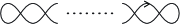
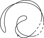
Figure 8. A chain-like curve and its realization with $i_{\gamma}=2$.

Example 2.12.

(Chain-like curves.) We consider a curve $\gamma$ with $\#_{\gamma}=n$ ($n\geq 1$) as in Figure 8, left. This curve has two shells and $n-1$ leaves, including a positive shell and a negative leaf, which are disjoint. Thus $(I(\gamma)\geq)\mu(\gamma)\geq 2$ holds. As in Figure 8, right, this curve can be drawn along a spiral with two inflections. So we can conclude that $I(\gamma)=\mu(\gamma)=2$. In this manner, drawing curves along a spiral is often useful to reduce the number of inflection points. Several useful techniques for drawing curves with a restricted number of inflections are mentioned in Halpern [6, Section 4].

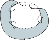
Figure 9. A figure of the curve $\gamma_{n}$.

Example 2.13.

(Curves with a negative $n$-gon.) We consider a curve $\gamma_{n}$ as in Figure 9, which has several positive polygons, but only one negative admissible $n$-gon, marked in gray in Figure 9. So we can conclude that $I(\gamma)=\mu(\gamma)=2$, as in Figure 9. This example shows that an $n$-gon $(n\geq 4)$ is needed to find a curve that cannot be locally convex.

Admissibility of a polygon is important for the definition of the invariant $\mu$. In fact, the curve as in Figure 10, left, has negative polygons which are not admissible, and it can be realized without inflections as in Figure 10, right.

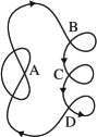
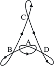
Figure 10. A curve satisfying $i_{\gamma}=0$.

Example 2.14.

(A curve with an effective leaf which is neither positive nor negative.) We consider a curve $\gamma$ as in Figure 11. This curve has $5$ crossings and exactly two positive shells at $A$ and $B$. It also has a negative shell at $C$. Thus $\mu\geq 2$ by Proposition 2.5. We show that $\mu(\gamma)=4$ by way of contradiction: There exist two positive points $p_{1}$ and $p_{2}$ on the two positive shells at $A$ and $B$, respectively. There is a unique simple closed arc $\Gamma$ bounded by $A$ and $B$ which passes through $D$ and $E$. Suppose that $\mu(\gamma)=2$. Then there are no negative points on $\Gamma$. Now we look at the negative leaf with vertices $A$ and $D$. In Figure 11, this leaf is marked in gray. Since $\Gamma$ does not contain a negative point, there must be a negative point $m_{1}$ between $A$ and $D$ on this leaf. Since the curve has a symmetry, applying the same argument to the negative leaf at $B$ and $E$, there is another negative point $m_{2}$ between $E$ and $C$.

Finally, we look at a leaf with vertices $D$ and $E$, which is not positive nor negative. Since $\Gamma$ has no negative point, there must have a positive point $p_{3}$ on the arc on the right-hand side of the leaf. Since the sequence $p_{1},m_{1},p_{3},m_{2},p_{2}$ changes sign four times, this gives a contradiction. Thus $\mu(\gamma)\geq 4$. Since the curve can be drawn with exactly four inflections as in Figure 11, we can conclude that $I(\gamma)=\mu(\gamma)=4$. In this example, an admissible polygon which is neither positive nor negative plays a crucial role to estimate the invariant $I(\gamma)$ by using $\mu(\gamma)$.

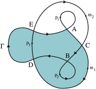
Figure 11. A curve satisfying $i_{\gamma}=4$ and $\#_{\gamma}=5$.

(Proof of the second assertion of Theorem 1.2.) The table of spherical curves up to $\#_{\gamma}\leq 5$ is given in the appendix of [7]. By moving the position of $\infty$ in $S^{2}=\bm{R}^{2}\cup\{\infty\}$, we get the table of planar curves up to $\#_{\gamma}\leq 5$ and can compute the invariant $\mu(\gamma)$. So we can list the curves with $\mu(\gamma)=0$. By Proposition 2.5, it is sufficient to check for the existence of positive polygons and negative polygons. When $\#_{\gamma}\leq 2$, the number of topological types of such curves is $3$. If $\#_{\gamma}=3,4,5$, then the number of topological types of such curves is $6,16,50$, respectively. After that we can draw the pictures of the curves by hand. If we are able to draw $76$ figures of the curves without inflections, the proof is finished, and this was accomplished in Figures 14, 16 and 17. ∎

(Proof of Corollary 1.3.) For curves $\gamma$ with $\mu(\gamma)=0$, we can show $I(\gamma)=0$ by drawing curves without inflections. On the other hand, when $\mu(\gamma)>0$, we can show $I(\gamma)=2$ by drawing curves with exactly two inflections, except for the curve as in Figure 4. ∎

3. Double tangents and geotopical tightness

In this section, we would like to give an application.

Definition 3.1.

Let $\gamma$ be a generic planar curve. We set

(3.1) $$d(\gamma):=d_{1}(\gamma)+d_{2}(\gamma).$$

Then we define

(3.2) $$\delta(\gamma):=\min_{\sigma\in\langle\gamma\rangle}d(\sigma),$$

which gives the minimum number of double tangents of the curves in the equivalence class $\langle\gamma\rangle$. (As in Figure 12, $d(\sigma)$ might be different from $d(\gamma)$ even if $\sigma\in\langle\gamma\rangle$ and $i_{\gamma}=i_{\sigma}=I(\gamma)$.) A curve $\sigma\in\langle\gamma\rangle$ satisfying $d(\gamma)=\delta(\gamma)$ is called geotopically tight or $g$-tight. We call the integer $\delta(\gamma)$ the $g$-tightness number.

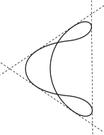
Figure 12. Curves of $2_{2}^{c}$ with $i_{\gamma}=2$ but with different $d$.

The following assertion holds:

Proposition 3.2.

It holds that $\delta(\gamma)\geq\#_{\gamma}+I(\gamma)/2$.

Proof.

By (0.1), we get that

$$d(\sigma)=d_{1}(\sigma)+d_{2}(\sigma)\geq d_{1}(\sigma)-d_{2}(\sigma)=\#_{\sigma}+\frac{I(\sigma)}{2}$$

holds for $\sigma\in\langle\gamma\rangle$. Taking the infimum, we get the assertion. ∎

We expect that any locally convex generic closed curves might be $g$-tight (see Question 4). Relating this, we can prove the following assertion:

Let $\gamma:\bm{R}\to\bm{R}^{2}$ be a periodic parametrization by arclength of a locally convex curve with total length $\ell$, that is, $\gamma(t+\ell)=\gamma(t)$ holds for $t\in\bm{R}$. Without loss of generality, we may assume that the curvature of $\gamma$ is positive. Let

$$x=\gamma(s_{1})=\gamma(s_{2})\qquad(0<|s_{1}-s_{2}|<\ell)$$

be a crossing of $\gamma$. Replacing $s_{1}$ by $s_{1}+\ell$ if necessary, we may assume that $s_{1}<s_{2}$ and $\dot{\gamma}(s_{2})$ is a positively rotated vector of $\dot{\gamma}(s_{1})$ through an angle $\alpha$ with $0<\alpha<\pi$. When the parameter $t$ varies in the interval $[s_{1},s_{2}]$, the tangent vector $\dot{\gamma}(t)$ rotates through an angle $2\pi n_{1}+\alpha$, where $n_{1}$ is a positive integer. Similarly, for the interval $[s_{2},s_{1}+\ell]$, there exists a positive integer $n_{2}$ such that the rotation angle of $\dot{\gamma}(t)$ is equal to $2\pi n_{2}-\alpha$. The sum $n_{1}+n_{2}$ is the total rotation index of $\gamma$. Denote by $W(x)$ the difference $n_{1}-n_{2}$. We easily recognize that the sum of $W(x)$ for each crossing $x$ of $\gamma$ is a geotopy invariant. The following theorem can be proved using the equality of $d_{2}$ in [8, p7] (we omit the details):

Theorem 3.3.

The number of double tangents for any locally convex generic closed curve $\gamma$ depends only on its geotopy type. More precisely, the following identity holds:

(3.3) $$d_{2}(\gamma)=\sum W(x),$$

where the sum runs over all crossings $x$ of $\gamma$.

Remark 3.4.

The rotation index $R_{\gamma}$ of $\gamma$ which is at each crossing equal to $n_{1}+n_{2}$, as mentioned above, is less than or equal to $\#_{\gamma}+1$ (cf. [W]). Thus the formula (3.3) implies

$$d_{2}=\#_{\gamma}R_{\gamma}-2\sum W(x)\leq\#_{\gamma}(\#_{\gamma}+1)-2\#_{\gamma}=\#_{\gamma}(\#_{\gamma}-1),$$

which reproves Halpern’s conjecture in [H2].

Corollary 3.5.

$\delta(\gamma)=1,2,2,3,3$ for $\gamma$ of type $1_{1},1_{1}^{b},1_{2},2_{2}^{b},2_{2}^{c}$ as in Figure 3, respectively.

Proof.

By Proposition 3.2, $\delta(\gamma)\geq 1,2,3,3$ for $\gamma$ of type $1^{b},2_{2}^{b},2_{2}^{c}$, respectively. On the other hand, the curves given in Figure 3 attain equality in this inequality. ∎

In Figure 3, there are two remaining curves of type $1_{2}^{b}$ and $2_{2}$, whose g-tightness numbers have not been specified by the authors. The curve of type $2_{2}$ given in Figure 3 satisfies $d(\gamma)=4$, and we expect that $\delta(\gamma)=4$. On the other hand, the corresponding curve as in the right of Figure 3 satisfies $d=7$, but one can realize the curve with $d=5$ as in Figure 1. We expect that it might be $g$-tight. If true, $\delta(\gamma)=5$ holds.

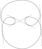
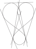
Figure 13. Curves of type $2_{2}$ and $1^{b}_{2}$.

A relationship between inflection points and double tangents for simple closed curves in the real projective plane with a suitable convexity is given in [11]. Finally, we leave several open questions on the invariants $I(\gamma)$ and $\delta(\gamma)$:

Question 1. Does $\mu(\gamma)=0$ imply $I(\gamma)=0$?

Question 2. Is there a generic closed curve satisfying $I(\gamma)>\mu(\gamma)$?

The authors do not know of any such examples. If we suppose $I(\gamma)=\mu(\gamma)$, then (2.2) yields the inequality $I(\gamma)\leq 2\#_{\gamma}$.

Question 3. Does $I(\gamma)\leq 2\#_{\gamma}$ hold for any generic closed curve in $\bm{R}^{2}$?

Question 4. Is an arbitrary locally convex curve $g$-tight?

Question 5. Find a criterion for $g$-tightness. For example, can one determine $\delta(\gamma)$ when $\gamma$ is of type $2_{2}$ or $1^{b}_{2}$?

Acknowledgements.

The authors thank Wayne Rossman for careful reading of the first draft and for giving valuable comments.

4. Tables of curves.

References

- [1] V. I. Arnold, Topological Invariants of Plane Curves and Caustics, University Lecture Series 5, American Mathematical Society, Providence, Rhode Island, 1994.
- [2] G. Cairns and D. M. Elton, The planarity problem for signed Gauss words, J. Knot Theory Ramifications 2 (1993), 359–367.
- [3] Fr. Fabricius-Bjerre, On the double tangents of plane closed curves, Math. Scand. 11 (1962), 113–116.
- [4] J. S. Carter, Classifying immersed curves, Proc. Amer. Math. Soc. 111 (1991), 281-287.
- [5] B. Halpern, Global theorems for closed plane curves, Bull. Amer. Math. Soc. 92 (1970), 96–100.
- [6] B. Halpern, An inequality for double tangents, Proc. Amer. Math. Soc. 76 (1979), 133–139.
- [7] O. Kobayashi and M. Umehara, Geometry of Scrolls, Osaka J. Math. 33 (1996), 441–473.
- [8] T. Ozawa, On Halpern’s conjecture for closed plane curves, Proc. Amer. Math. Soc 92 (1984), 554–560.
- [9] T. Ozawa, Topology of Planar Figures, Lecture Notes in Math. 9 Bifukan Inc. (in Japanese) 92 (1997).
- [10]
- [11] G. Thorbergsson and M. Umehara, Inflection points and double tangents on anti-convex curves in real projective plane, Tohoku Math. J. 60 (2008), 149–181.
- [12] M. Umehara, -vertex theorem for closed planar curve which bounds an immersed surface with non-zero genus, Nagoya Math. J. 134 (1994) 75-89.
- [13] H. Whitney, On regular closed curves on plane, Compositio Math. 4 (1937) 276–284.