Waltzing peakons and compacton pairs in a cross-coupled Camassa-Holm equation

Abstract

We consider singular solutions of a system of two cross-coupled Camassa-Holm (CCCH) equations. This CCCH system admits peakon solutions, but it is not in the two-component CH integrable hierarchy. The system is a pair of coupled Hamiltonian partial differential equations for two types of solutions on the real line, each of which separately possesses $\exp(-|x|)$ peakon solutions with a discontinuity in the first derivative at the peak. However, there are no self-interactions, so each of the two types of peakon solutions moves only under the induced velocity of the other type. We analyse the ‘waltzing’ solution behaviour of the cases with a single bound peakon pair (a peakon couple), as well as the over-taking collisions of peakon couples and the antisymmetric case of the head-on collision of a peakon couple and a peakon anti-couple. We then present numerical solutions of these collisions, which are inelastic because the waltzing peakon couples each possess an internal degree of freedom corresponding to their ‘tempo’ – that is, the period at which the two peakons of opposite type in the couple cycle around each other in phase space. Finally, we discuss compacton couple solutions of the cross-coupled Euler-Poincaré (CCEP) equations and illustrate the same types of collisions as for peakon couples, with triangular and parabolic compacton couples. We finish with a number of outstanding questions and challenges remaining for understanding couple dynamics of the CCCH and CCEP equations.

, , , ,

AMS Classification:

Keywords:

1 Introduction

1.1 Purpose and scope of the paper

In this paper we investigate solution properties of a new two-component Camassa-Holm (CH) system introduced in equations (13) and (14). As far as we know, this system is not completely integrable. However, the system does possess bound pairs of peakon solutions which exhibit interesting propagation dynamics involving both propagation and oscillation, while a single peakon must remain stationary (fixed in space). The oscillating and translating motion of the bound pairs of peakons as they propagate is reminiscent of the swirling motion of waltzing dancers, so we call these solutions peakon couples. The variational derivation of the equations, their geometry and the behaviour of the peakon couple propagation and collision interactions are studied in the paper. We also discuss compacton couple solutions for the more general case of cross-coupled Euler-Poincaré (CCEP) equations in (13) and (14), and illustrate the same types of collisions as for peakon couples, with triangular and parabolic compacton couples.

CH equation and generalizations

The well-known CH equation may be written as [2, 3]

$$u_{t}-u_{xxt}+2\omega u_{x}+3uu_{x}-2u_{x}u_{xx}-uu_{xxx}=0,$$ (1)

where subscripts denote partial derivatives of the horizontal fluid velocity $u(x,t)$ and the linear dispersion parameter $\omega$ is a real constant. The solution $u(x,\,\cdot\,)$ and its derivative $u_{x}(x,\,\cdot\,)$ are assumed to vanish sufficiently rapidly at spatial infinity, $\lim_{|x|\to\infty}(u,u_{x})(x,\,\cdot\,)=0$.

The integrable CH equation (1) describes the unidirectional propagation of shallow water waves over a flat bottom at one order in asymptotic expansion beyond the KdV equation [2, 3, 8, 9, 21, 22, 5]. The CH equation also governs axially symmetric waves in a hyperelastic rod [7]. In the case of no linear dispersion, $\omega=0$, the CH equation (1) possesses singular solutions in the form of peaked travelling waves called peakons

$$u(x,t)=\frac{c}{2}\exp({-|x-ct|})\,.$$ (2)

Peakon properties and solution behaviour are reviewed in [11]. Recent developments about the CH equation may also be found in [18, 12] and the references therein.

The scope of mathematical interpretations of CH may be gleaned by rewriting it in various equivalent forms, many of which have been rediscovered several times and each of which can be a point of departure for further investigation. For example, CH may be treated variously as: a fluid motion equation; a mathematical model of shallow water wave breaking; a transport equation for wave momentum by a fluid velocity related to it by inversion of the Helmholtz operator; a nonlocal characteristic equation; an Euler-Poincaré equation describing geodesic motion on the diffeomorphism group with respect to the metric defined by the $H^{1}$ norm on the tangent space of vector fields; a Lie-Poisson Hamiltonian system describing coadjoint motion on the Bott-Virasoro Lie group; a bi-Hamiltonian system; a compatibility equation for a linear system of two equations in a Lax pair, etc.

In particular, the CH equation on the real line follows from Hamilton’s principle $\delta{S}=0$ with an action $S=\int l(u)dt$ given by Lagrangian

$$l(u)=\frac{1}{2}\int u^{2}+2\omega{u}+u_{x}^{2}\,dx$$ (3)

for solutions $u(x,t)$ that vanish sufficiently rapidly at spatial infinity. The Euler-Poincaré equation [16]

$${\partial_{t}}m=-\,{\rm ad}^{*}_{u}m=-\,(um)_{x}-mu_{x}\quad\hbox{with}\quad m:=\frac{\delta l}{\delta u}=u-u_{xx}+\omega,$$ (4)

then recovers the CH equation (1).

The present paper emerged from the observation that complexifying the CH Lagrangian in (3) yields

$$l(u,v) = \frac{1}{2}\int(u+iv)^{2}+2\omega(u+iv)+(u_{x}+iv_{x})^{2}\,dx$$

$$= \frac{1}{2}\int(u^{2}+u_{x}^{2})+2\omega{u}+(v^{2}+v_{x}^{2})\,dx+i\int uv+u_{x}v_{x}+\omega{v}\,dx$$

$$= \Re(l)+i\,\Im(l).$$

Now the Euler-Poincaré equation (4) for the real part of the Lagrangian $\Re(l)$ simply yields two separate copies of the CH equation, one with $\omega$ and one without. This, of course, is of no further interest, because it gives nothing new. However, the Euler-Poincaré equation for the imaginary part of the Lagrangian $\Im(l)$ yields a new coupled system of two equations for $u$ and $v$ that we shall investigate in the remainder of the present paper. This system of cross-coupled CH equations (CCCH) is found to be (with details of the derivation given in Section 3)

$${\partial_{t}}m = -\,{\rm ad}^{*}_{v}m=-\,(vm)_{x}-mv_{x}\quad\hbox{with}\quad m:=\frac{\delta l}{\delta v}=u-u_{xx}+\omega,$$ (6)

$${\partial_{t}}n = -\,{\rm ad}^{*}_{u}n=-\,(un)_{x}-nu_{x}\quad\hbox{with}\quad n:=\frac{\delta l}{\delta u}=v-v_{xx}.$$ (7)

In these equations the momentum $m$ (resp. $n$) is transported only by the opposite induced velocity $v$ (resp. $u$). Hereafter, we ignore linear dispersion by setting set $\omega=0$. This has the effect that: (i) the system is symmetric and (ii) it admits peakon solutions. Peakon solutions for the CCCH system (6) and (7) with $\omega=0$ are singular solutions in which the values of the momenta $m$ and $n$ are supported with time-dependent weights on delta functions at points moving along the real line, carried by the appropriate velocity.

The present paper focuses its attention on the dispersionless cross-coupled CH system (CCCH) comprising (6) and (7) with $\omega=0$. These equations govern two types of peakons. Each type of peakon is swept along by the induced flow of other peakons of the opposite type. We also consider solutions of the cross-coupled Euler-Poincaré equations CCEP,

$${\partial_{t}}m = -\,{\rm ad}^{*}_{v}m=-\,(vm)_{x}-mv_{x}\quad\hbox{with}\quad u=K_{\mathcal{G}}*m,$$ (8)

$${\partial_{t}}n = -\,{\rm ad}^{*}_{u}n=-\,(un)_{x}-nu_{x}\quad\hbox{with}\quad v=K_{\mathcal{G}}*n.$$ (9)

For a convolution kernel $K_{\mathcal{G}}(\,\cdot\,)$ with compact spatial support, these CCEP equations admit compacton solutions whose scattering interactions we shall compute.

To finish establishing the notation, the next paragraph will quickly review the well-known behaviour of the CH equation by writing in several of its various forms and discussing its properties that will be relevant here, in parallel with the properties of the CCCH system (6) and (7). We should mention that there are other, integrable two and multi-component CH systems with application in fluid mechanics, see e.g. [23, 4, 19, 10, 6, 17, 20, 14, 13].

1.2 Parallel properties for CH and CCCH

Momentum conservation in CH and CCCH.

The CH equation (1) with $\omega=0$

$$u_{t}-u_{xxt}+3uu_{x}-2u_{x}u_{xx}-uu_{xxx}=0,$$ (10)

may be rewritten in the form of a momentum conservation law, as

$$u_{t}+\partial_{x}\left(\frac{1}{2}u^{2}+P\right)=0\,,$$ (11)

with pressure $P$ given by the convolution

$$P=K*\left(u^{2}+\frac{1}{2}u_{x}^{2}\right)\quad\hbox{with kernel}\quad K(x,y)=\frac{1}{2}\exp(-|x-y|).$$ (12)

The kernel $K$ for peakons is the Green’s function for the 1D Helmholtz operator, $(1-\partial_{x}^{2})$, and is also the shape of the peakon velocity profile in (2).

When expressed in terms of the corresponding velocities $u=K*m$ and $v=K*n$, with kernel $K(x)$ given by the Green’s function in equation (12), the cross-coupled CH (CCCH) equations (6) and (7) with $\omega=0$ expand into

$$u_{t}-u_{xxt}+vu_{x}+2v_{x}u-2v_{x}u_{xx}-vu_{xxx} = 0,$$ (13)

$$v_{t}-v_{xxt}+uv_{x}+2u_{x}v-2u_{x}v_{xx}-uv_{xxx} = 0,$$ (14)

As for CH, the total momentum of CCCH is conserved, namely

$$\partial_{t}\left(u+v\right)+\partial_{x}\big{(}uv+K*(2uv+u_{x}v_{x})\big{)}=0.$$ (15)

Characteristic forms of CH and CCCH.

The CH equation (10) may be interpreted as the condition for the 1-form density $m\,dx^{2}$ to be preserved (or ‘frozen’) in the flow of the characteristic velocity $dx/dt=u(x(t),t)$, namely,

$$\frac{d}{dt}\Big{(}m\,dx^{2}\Big{)}=0\,,\quad\hbox{along}\quad\frac{dx}{dt}=u(x(t),t)=K*m.$$ (16)

Note that the relation between the velocity of the flow $u$ and the property that it carries $m$ is nonlocal.

Likewise, for the CCCH equations, but with the cross velocities, we have

$$\frac{d}{dt}\Big{(}m\,dx^{2}\Big{)} = 0\,,\quad\hbox{along}\quad\frac{dx}{dt}=v(x(t),t)=K*n,$$ (17)

$$\frac{d}{dt}\Big{(}n\,dx^{2}\Big{)} = 0\,,\quad\hbox{along}\quad\frac{dx}{dt}=u(x(t),t)=K*m,$$ (18)

where again the characteristic velocities depend nonlocally on the quantities that they carry. These formulas imply that the signs of the momenta $m$ and $n$ are preserved along characteristics during the motion. In particular, if the initial conditions for either of the momenta $m$ and $n$ are everywhere positive, then the sign of that momentum is preserved throughout the subsequent evolution.

Multi-peakon solutions of CH and CCCH.

For CH, the velocity is related to the momentum by convolution with the kernel $K$ in (12), which is the Greens function for the Helmholtz operator. When expressed in terms of the momentum, the multi-peakon solution of CH for $\omega=0$ is a sum over delta functions, supported on a set of points moving on the real line. That is, CH for $\omega=0$ has solutions for velocity and momenta given, respectively, by

$$u(x,t)=\sum_{a=1}^{N}\,p_{a}(t)e^{-|x-q_{a}(t)|}\quad\hbox{and}\quad m(x,t)=\sum_{a=1}^{N}\,p_{a}(t)\delta(x-q_{a}(t))\,.$$ (19)

As shown in [15], the CH peakon solution (19) is geometrically the cotangent-lift momentum map for the left action of the diffeomorphisms ${\rm Diff}(\mathbb{R})$ on a set of $N$ points on the real line. The same momentum map applies for CCCH, resulting in the peakon solutions, with velocities

$$u(x,t)=\frac{1}{2}\sum_{a=1}^{M}m_{a}(t)\,e^{-|x-q_{a}(t)|}\,,\qquad v(x,t)=\frac{1}{2}\sum_{b=1}^{N}n_{b}(t)\,e^{-|x-r_{b}(t)|}\,,$$ (20)

and momenta supported on delta functions moving along the real line,

$$m(x,t)=\sum_{a=1}^{M}m_{a}(t)\,\delta(x-q_{a}(t))\,,\qquad n(x,t)=\sum_{b=1}^{N}n_{b}(t)\,\delta(x-r_{b}(t))\,.$$ (21)

The dynamics of the CCCH equations and their peakon solutions will be the focus of the remainder of the paper.

1.3 Main content of the paper

Section 2 studies the two-component solutions of the CCCH equations (13) and (14). This is done first in a numerical solution of their partial differential equations that establishes their characteristic wave behaviour in the classic dam-break problem for water waves. Then the study of their peakon solutions begins.

Section 3 derives the system of cross-coupled CH (CCCH) equations in (6) and (7) from a variational principle on the direct-product space of $C^{0}$ vector fields $\mathfrak{X}(\mathbb{R})\times\mathfrak{X}(\mathbb{R})$.

Section 4 discusses $N$-peakon solutions of the CCCH system.

Section 5 studies the simplest possible case, $M=N=1$. This is the peakon couple solution for CCCH.

Section 6 discusses the periodic equilibrium solutions of the CCCH system.

Section 7 considers the anti-symmetric collision of a CCCH peakon couple with its spatial reflection.

Section 8 presents the results of numerical integrations of the interactions between the cross-coupled peakon couple and other coherent couple structures for CCCH.

Section 9 studies compacton-couple solutions of the CCEP system (8) and (9). The dynamics of these compacton couples have some interesting features that depend on the shapes of their profiles. We study triangular and parabolic profiles.

Section 11 recaps the main results of the paper and lists some of the outstanding problems remaining for future investigations of the CCCH and CCEP equations.

2 Two-component solutions of the CCCH equations

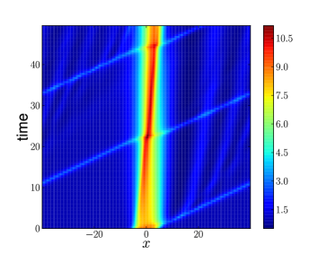
(a) (b)

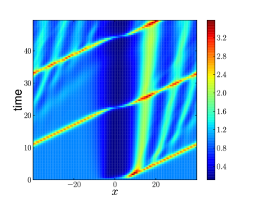
Figure 1: Spacetime plots of the dam-break solution behaviour of the velocity variables, $v$ (Panel a) and $u$ (Panel b) of the cross-coupled equations (13, 14) for initial conditions (22) with tanh-squared profile and disturbance width 10 units. The subsequent flow is calculated numerically in a periodic domain of width 80 units. As in the classical Saint Venant shallow water problem, wave-like phenomena are created at the moment of release, though the waves propagate only in a rightward direction due to positive mean velocities.

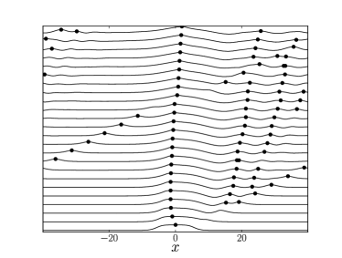
(a) (b)

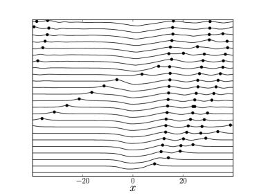
Figure 2: Waterfall plots for the dam-break solution behaviour of the velocity variables $v$ (Panel a) and $u$ (Panel b) of the cross-coupled equations (13, 14) for the same data as Figure 1. Solutions at intervals of 3 time units are plotted sequentially up the page and the dots identify locations of the three highest local maxima at each time interval.
Panel (a) shows the creation of a slow main excitation, a faster excitation and a few slower subsidiary excitations that branch off from it.
Panel (b) shows a fast rightward moving excitation induced by the development of the first fast excitation in the left panel, and several slow subsidiary excitations that branch off from it.
Both of these excitations are coherent structures that seem to retain their identities after the collision with each other in the middle of the figure. However, no compelling evidence about the integrability of the CCCH system can be drawn from this data.

‘Dam-break’ equivalent problem for the cross-coupled equations.

The dam-break problem involves a body of water of uniform depth, initially retained behind a barrier, in this case at $x=\pm 5$ in a periodic domain of width 80 units. When the barrier is suddenly removed at $t=0$, the water flows downward and outward under gravity. The problem is to find the subsequent flow and determine the shape of the free surface. This question was addressed in the context of shallow-water theory, e.g., by Acheson [1]. The dam-break results for the cross-coupled system in (13)-(14) in Figure 1 show evolution of the variables $v$ (left panel) and $u$ (right panel), arising from initial conditions in a periodic domain, in which an initially localized disturbance with tanh-squared profile in the momentum variable $n$ interacts with an initially constant mean flow in the independent cross-coupled velocity field, $u$. That is,

$$n(x,0) = \left[1+\tanh\left(x+5\right)-\tanh\left(x-5\right)\right]^{2},$$ (22)

$$m(x,0) = u(x,0)=1.$$

This dam-break initial condition first spawns a rapid leading pulse in velocity $u$ and then produces a series of slower pulses in $u$, some of which are of larger amplitude than the first pulse. The rapid first pulse in $u$ then passes again through the periodic domain, overtaking and colliding with the series of slower but larger pulses and undergoing a strong interaction indicated by a burst of amplitude in each collision. The $u$ pulse and the $v$ pulse track each other, but their variations have opposite phase. That is, a maximum in the $u$ pulse corresponds to a minimum in the $v$ pulse, and vice versa. This is an interesting scenario that we will see emerging when we study the coupled peakon solutions.

3 Variational derivation of the CCCH and CCEP equations

In this section we derive the CCCH and CCEP equations (6) and (7) from Hamilton’s principle, by using the Euler-Poincaré theory for symmetry reduction of right-invariant Lagrangians defined on the tangent space of a Lie group. We begin by considering motion on the direct product of two copies of the smooth invertible maps with smooth inverses (diffeomeorphisms) acting on the real line ${\rm Diff}(\mathbb{R})\times{\rm Diff}(\mathbb{R})$. We consider a reduced Lagrangian $l({u},v):\,\mathfrak{X}(\mathbb{R})\times\mathfrak{X}(\mathbb{R})\to\mathbb{R}$ that depends on a pair of smooth vector fields $({u},v)\in\mathfrak{X}(\mathbb{R})=T_{e}{\rm Diff}(\mathbb{R})/{\rm Diff}(\mathbb{R})$ that are right-invariant under ${\rm Diff}(\mathbb{R})$. Applying the standard calculation of Hamilton’s principle for this right-invariant Lagrangian yields, see e.g. [16, 18],

$$\delta\int_{a}^{b}l({u},v)dt = \int_{a}^{b}\left\langle\frac{\delta l}{\delta{u}},\delta{u}\right\rangle+\left\langle\frac{\delta l}{\delta{v}},\delta{v}\right\rangle dt$$

$$= \int_{a}^{b}\left\langle\frac{\delta l}{\delta{u}}\,,\,\frac{d\eta}{dt}-{\rm ad}_{u}{\eta}\right\rangle+\left\langle\frac{\delta l}{\delta{v}}\,,\,\frac{d\xi}{dt}-{\rm ad}_{v}{\xi}\right\rangle dt$$

$$= -\int_{a}^{b}\,\left\langle\frac{d}{dt}\frac{\delta l}{\delta{u}}+{\rm ad}_{u}^{*}\frac{\delta l}{\delta{u}}\,,\,{\eta}\right\rangle+\left\langle\frac{d}{dt}\frac{\delta l}{\delta{v}}+{\rm ad}_{v}^{*}\frac{\delta l}{\delta{v}}\,,\,{\xi}\right\rangle\,\,dt\,,$$

where one invokes $\eta=0$ and $\xi=0$ for the variations in $\mathfrak{X}(\mathbb{R})$ vanishing at the endpoints in time when integrating by parts and takes the continuum velocity vector fields $({u},v)\in\mathfrak{X}(\mathbb{R})$ to vanish asymptotically in space. We have also used the formulas

$$\delta{u}=\frac{d\eta}{dt}-{\rm ad}_{u}{\eta}\,,\qquad\delta{v}=\frac{d\xi}{dt}-{\rm ad}_{v}{\xi}\,,\quad\hbox{with}\quad\eta,\ \xi\in\mathfrak{X}(\mathbb{R})\,,$$ (23)

for the variation of the right-invariant vectors field $(u,v)$ and have taken the pairing

$$\langle\,\cdot\,,\,\cdot\,\rangle:\,\mathfrak{X}(\mathbb{R})\times\mathfrak{X}^{*}(\mathbb{R})\to\mathbb{R}$$

as the $L^{2}$ pairing between elements of the Lie algebra $\mathfrak{X}(\mathbb{R})$ and its dual $\mathfrak{X}^{*}(\mathbb{R})$, the space of smooth 1-form densities. This pairing allows us to define the ${\rm ad}^{*}$-operation as

$$\left\langle{\rm ad}_{v}^{*}\frac{\delta l}{\delta{v}}\,,\,{\xi}\right\rangle=\left\langle\frac{\delta l}{\delta{v}}\,,\,{\rm ad}_{v}{\xi}\right\rangle,$$ (24)

where

$${\rm ad}_{v}{\xi}:=-[v,\xi]:=-v\xi_{x}+\xi v_{x}$$ (25)

is the adjoint Lie-algebra action $\mathfrak{X}(\mathbb{R})\times\mathfrak{X}(\mathbb{R})\to\mathfrak{X}(\mathbb{R})$, given by minus the Jacobi-Lie, or commutator bracket of smooth vector fields. In our case, $\langle\cdot\,,\,\cdot\rangle$ is the $L^{2}$ pairing between vector fields $\mathfrak{X}(\mathbb{R})$ and 1-form densities $\mathfrak{X}^{*}(\mathbb{R})$, written as

$$\left\langle\frac{\delta l}{\delta{u}},\delta{u}\right\rangle=\int\delta{u}\,\frac{\delta l}{\delta{u}}\,dx,$$

in which the integral is taken over the infinite real line.

Substituting the reduced Legendre transformation $u\mapsto\mu=\delta\ell/\delta u$ and $v\mapsto\nu=\delta\ell/\delta v$ produces the following pair of Euler-Poincaré equations governing coadjoint motion for $(\mu,\nu)\in\mathfrak{X}^{*}(\mathbb{R})\times\mathfrak{X}^{*}(\mathbb{R})$,

$$\partial_{t}\mu+{\rm ad}_{u}^{*}\mu=0\,,\quad\partial_{t}\nu+{\rm ad}_{v}^{*}\nu=0\quad\hbox{for}\quad\mu:=\delta l/\delta{u}\,,\quad\nu:=\delta l/\delta{v}\,.$$ (26)

We may evaluate the ${\rm ad}^{*}$-expressions from their definitions, so that

$$\left\langle{\rm ad}^{*}\mu\,,\,{\xi}\right\rangle=\left\langle\mu\,,\,{\rm ad}_{u}{\xi}\right\rangle=\left\langle\mu\,,\,-u\xi_{x}+\xi u_{x}\right\rangle=\left\langle(\mu u)_{x}+\mu u_{x},\,\xi\right\rangle\,,$$

and similarly for $(\mu,u)\to(\nu,v)$. These expressions yield the Euler-Poincaré equations on the real line for an arbitrary right-invariant Lagrangian.

If the reduced Legendre transformation $(u,v)\mapsto(\mu,\nu)$ is invertible, then the Euler-Poincaré equations (26) are equivalent to the (right) Lie-Poisson Hamiltonian equations:

$$\dot{\mu}=-{\rm ad}^{*}_{\delta h/\delta\mu}\mu\,,\quad\dot{\nu}=-{\rm ad}^{*}_{\delta h/\delta\nu}\nu\,,$$ (27)

where the reduced Hamiltonian $h$ and its variational derivatives are obtained from the reduced Legendre transformation by

$$h(\mu,\nu)=\left\langle\mu,u\right\rangle+\left\langle\nu,v\right\rangle-l({u},v).$$

These equations are equivalent (via Lie-Poisson reduction and reconstruction) to Hamilton’s equations on $T^{\ast}{\rm Diff}\times T^{\ast}{\rm Diff}$ relative to the Hamiltonian $H:T^{\ast}{\rm Diff}\times T^{\ast}{\rm Diff}\rightarrow\mathbb{R}$, obtained by right translating $h$ from the identity element to other points via the right (diagonal) action of ${\rm Diff}$ on $T^{\ast}{\rm Diff}\times T^{\ast}{\rm Diff}$. The Lie-Poisson equations may be written in the Poisson bracket form

$$\dot{F}(\mu,\nu)=\left\{F,h\right\},$$ (28)

where $F:\mathfrak{X}^{*}\times\mathfrak{X}^{*}\rightarrow\mathbb{R}$ is an arbitrary smooth function and the bracket is the (right) Lie-Poisson bracket given by

$$\{F,G\}(\mu,\nu)=\left\langle\mu,\left[\frac{\delta F}{\delta\mu},\frac{\delta G}{\delta\mu}\right]\right\rangle+\left\langle\nu,\left[\frac{\delta F}{\delta\nu},\frac{\delta G}{\delta\nu}\right]\right\rangle.$$ (29)

In the cases we shall consider, the Lagrangian $l(u,v)$ will be bilinear, and its variations will cross-couple the momentum equations, as follows. An arbitrary norm on the tangent space of vector fields, $\left\|u\right\|=\left\langle\,u,\mathcal{G}u\right\rangle,$ with $\mathcal{G}$ a positive symmetric operator on $u$, induces cross-coupled equations through the application of the Euler-Poincaré framework to the new Lagrangian $l_{\mathcal{G}}\left(u,v\right)=\left\langle\,u,\mathcal{G}v\right\rangle=\left\langle\,\mathcal{G}u,v\right\rangle.$ In particular, the momenta in the Legendre transformation are given by,

$$\mu=\frac{\delta l_{\mathcal{G}}}{\delta u}=\mathcal{G}v\quad\hbox{and}\quad\nu=\frac{\delta l_{\mathcal{G}}}{\delta v}=\mathcal{G}u.$$

The corresponding Hamiltonian is given by

$$h_{\mathcal{G}}(\mu,\nu)=\left\langle\,K_{\mathcal{G}}*\mu,\nu\right\rangle=\left\langle\,K_{\mathcal{G}}*\nu,\mu\right\rangle$$

by symmetry of the kernel $K_{\mathcal{G}}$. Consequently, the associated velocities are obtained from the convolutions

$$\frac{\delta h_{\mathcal{G}}}{\delta\mu}=K_{\mathcal{G}}*\nu=u\quad\hbox{and}\quad\frac{\delta h_{\mathcal{G}}}{\delta\nu}=K_{\mathcal{G}}*\mu=v$$

in which the kernel $K_{\mathcal{G}}$ for the system is the Greens function for the invertible operator $\mathcal{G}$. The resulting Euler-Poincaré or Lie-Poisson equations may both be expressed as

$$\partial_{t}\mathcal{G}v+{\rm ad}_{u}^{*}\mathcal{G}v=0\,,\quad\partial_{t}\mathcal{G}u+{\rm ad}_{v}^{*}\mathcal{G}u=0\,.$$ (30)

These are the equations of the CCEP system (8) and (9) for a general choice of the operator $\mathcal{G}$ and its Greens function kernel $K_{\mathcal{G}}$. They will be the CCCH equations (6) and (7) with $\omega=0$, for the choice of the Helmholtz operator, $\mathcal{G}=1-\partial_{x}^{2}$.

Let us consider a few choices of the bilinear reduced Lagrangian $\ell({u},v)$ whose Euler-Poincaré equations (30) support peakon solutions on the real line:

1. When the reduced Lagrangian depends on only one vector field as $\ell({u})=\frac{1}{2}\|{u}\|_{H^{1}}^{2}$, then the dispersionless CH equation,

   $$\partial_{t}m+um_{x}+2mu_{x}=0\,,\quad\hbox{with}\quad m=u-u_{xx},$$

   emerges as the dynamics of geodesic motion on the diffeomorphisms with respect to the $H^{1}$ norm $\|{u}\|_{H^{1}}=\int u^{2}+u_{x}^{2}\,dx$.

2. When the reduced Lagrangian is taken as $\ell({u},v)=\int uv+u_{x}v_{x}\,dx$, we find the following pair of coupled Euler-Poincaré equations, in this case for the symmetric positive operator $\mathcal{G}=1-\partial_{x}^{2}$, the Helmholtz operator,

   $$\partial_{t}m+2v_{x}m+vm_{x}=0\,,\qquad\partial_{t}n+2u_{x}n+un_{x}=0\,,$$ (31)

   with $m=\delta l/\delta{v}=u-u_{xx}=\mathcal{G}u$ and $n=\delta l/\delta{u}=v-v_{xx}=\mathcal{G}v$. Because the momentum density ($m$) for one velocity vector field ($v$) is Lie-dragged by the vector field ($u$) for the other momentum density ($n$), we call this system the cross-coupled equations. When $v=u$, this coupled system restricts to the dispersionless CH equation. (Dispersion may be introduced by adding constant shifts to variables $m=u-u_{xx}+\omega_{1}$ and $n=v-v_{xx}+\omega_{2}$.)

3. When $(u,v)\in\mathbb{C}$ and $v=\bar{u}$, the reduced Lagrangian becomes the complex $H^{1}$ norm $\ell({u})=\int(|u|^{2}+|u_{x}|^{2})\,dx$ and we may interpret the coupled system of cross-coupled equations (31) as the complex version of the dispersionless CH equation.

4. The system of cross-coupled equations (31) may be written in Lie-derivative form as

   $$(\partial_{t}+\mathcal{L}_{v})\big{(}m\,dx^{2}\big{)}=0\quad\hbox{and}\quad(\partial_{t}+\mathcal{L}_{u})\big{(}n\,dx^{2}\big{)}=0\,,$$ (32)

   with two characteristic velocities, $u=K*m$ and $v=K*n$, in which the kernel $K$ is the Green’s function for the Helmholtz operator, defined in (12). The cross-coupled equations may also be written equivalently in a form similar to equation (18), as follows,

   $$\frac{d}{dt}\big{(}m\,dx^{2}\big{)} = 0\quad\hbox{along}\quad\frac{d{x}}{dt}={v({x},t)}=K*n\,,$$ (33)

   $$\frac{d}{dt}\big{(}n\,dx^{2}\big{)} = 0\quad\hbox{along}\quad\frac{d{x}}{dt}={u({x},t)}=K*m\,.$$ (34)

   These equivalent forms of the cross-coupled equations imply they admit particle-like delta function solutions for both $m$ and $n$, as discussed in the next section.

The remainder of the paper is devoted to studying the solutions of the CCCH system (31) and the more general CCEP system (30).

4 Peakon solutions of the cross-coupled equations

We have already asserted that the solutions of the CCCH system (31) may be expressed in the form (21) for the two momenta and (20) for their corresponding velocities. The delta-function representation of these momentum solutions is also the cotangent lift momentum map for the direct product ${\rm Diff}(\mathbb{R})\times{\rm Diff}(\mathbb{R})$ of diffeomorphisms acting on the real line $\mathbb{R}$ by composition from the left [15].

By general principles for momentum maps and in parallel with the peakon dynamics for the CH equation, the $2M+2N$ variables $(q_{a},m_{a})$, $a=1,\dots,M$, and $(r_{b},n_{b})$, $b=1,\dots,N$, in the peakon solutions for position (20) and momentum (21) of the CCCH equations (13, 14) are governed by Hamilton’s canonical equations for the Hamiltonian function,

$$H=\frac{1}{2}\sum_{a,b=1}^{M,N}m_{a}(t)n_{b}(t)e^{-|q_{a}(t)-r_{b}(t)|}\,.$$ (35)

These canonical equations comprise the evolution equations,

$$\dot{q}_{a}(t) = \frac{\partial H}{\partial m_{a}}=\frac{1}{2}\sum_{b=1}^{N}n_{b}(t)e^{-|q_{a}(t)-r_{b}(t)|}=v(q_{a}(t),t)\,,$$ (36)

$$\dot{r}_{b}(t) = \frac{\partial H}{\partial n_{b}}=\frac{1}{2}\sum_{a=1}^{M}m_{a}(t)e^{-|q_{a}(t)-r_{b}(t)|}=u(r_{b}(t),t)\,,$$ (37)

for the positions of the peakons, and

$$\dot{m}_{a}(t) = -\,\frac{\partial H}{\partial q_{a}}=\frac{1}{2}m_{a}\sum_{b=1}^{N}n_{b}\,{\rm sgn}\,(q_{a}-r_{b})e^{-|q_{a}(t)-r_{b}(t)|}=-\,m_{a}\,\frac{\partial v}{\partial x}\Big{|}_{x=q_{a}}\,,$$ (38)

$$\dot{n}_{b}(t) = -\,\frac{\partial H}{\partial r_{b}}=-\frac{1}{2}n_{b}\sum_{a=1}^{M}m_{a}\,{\rm sgn}\,(q_{a}-r_{b})e^{-|q_{a}(t)-r_{b}(t)|}=-\,n_{b}\,\frac{\partial u}{\partial x}\Big{|}_{x=r_{b}}\,,$$ (39)

for their canonical momenta. In the case originally envisioned that the solutions would be complex, for $v=\bar{u}\in\mathbb{C}$ we have $N=M$ and $n_{a}=\bar{m}_{a}$.

Conserved quantities for these equations include the energy $H$ and the total momentum $\sum_{a}(m_{a}+n_{a})$. The solutions of these peakon equations will be studied in more detail in the sections that follow.

5 The Peakon Dipole Solution

In this section, we consider the peakon solutions of the CCCH system in the simplest possible case, $M=N=1$. Dropping superfluous indices for this case, we introduce new canonical position variables $X=\left(q+r\right)/2$, $Y=q-r$, respectively mean position of the peaks and their separation distance. The evolution equations in terms of the new variables are

$$\dot{X}=\frac{\left(m+n\right)}{4}e^{-|Y|},$$

$$\dot{Y}=\frac{\left(n-m\right)}{2}e^{-|Y|}.$$

Thus we can define the behaviour of the exponential function of the absolute separation of the peaks,

$$\frac{d}{dt}e^{|Y|}=\mbox{sgn}\left(Y\right)\frac{\left(n-m\right)}{2},$$ (40)

where $\mbox{sgn}\left(x\right)$ denotes the signum function

$$\mbox{sgn}\left(x\right)=\theta\left(x\right)-\theta\left(-x\right)=\left\{\begin{array}[]{cc}1&\hbox{for }x>0,\\ -1&\hbox{for }x<0.\end{array}\right.$$

Meanwhile

$$\dot{m}=-\dot{n}=\mbox{sgn}\left(Y\right)\frac{mn}{2}e^{-|Y|}=\mbox{sgn}\left(Y\right)E,$$ (41)

where E=$\left.H\right|_{t=0}$is the (constant) value of the Hamiltonian, that is to say the total energy of the coupled pair. Differentiating (40) again with respect to time gives

$$\frac{d^{2}}{dt^{2}}\left(e^{|Y|}\right)=-\mbox{sgn}^{2}\left(Y\right)E+\delta\left(Y\right)\left(n-m\right)^{2}.$$

On integrating for a particular signature of $\left.Y\right|_{t=0}=Y_{0}\neq 0$,

$$e^{|Y|}=-\,\frac{m_{0}n_{0}e^{-|Y_{0}|}t^{2}}{2}+\mbox{sgn}\left(Y_{0}\right)\frac{\left(n_{0}-m_{0}\right)}{2}t+e^{|Y_{0}|},$$ (42)

where

$$m_{0}=\left.m\right|_{t=0},\quad n_{0}=\left.n\right|_{t=0}\quad Y_{0}=\left.Y\right|_{t=0}.$$

If $m_{0}$ and $n_{0}$ have the same signature, then eventually we will have $|Y|=0$, regardless of the value of $|Y_{0}|$. If $m_{0}$ and $n_{0}$ are of different signature, then provided $\mbox{sgn}\left(Y_{0}\right)\left(n_{0}-m_{0}\right)<0$ the same fate will occur. If the signatures differ and $\mbox{sgn}\left(Y_{0}\right)\left(n_{0}-m_{0}\right)>0$ then the particles immediately separate and continue to do so subject to the logarithmic rate of equation (42). In this case the amplitudes of both particles grow linearly according to equation (41).

At the point of collision when $|Y|=0$ we require both $H=\frac{1}{2}mn$ and $\mathcal{M}=m+n$ to be conserved. Thus the absolute value of $m-n$ is also conserved. If the particles are assumed to ‘tunnel’ through each other then the momenta are conserved and the signature of the whole problem in $Y$ switches, with the forcing on the amplitudes of the momenta reversed. Equivalently the particles can be assumed to collide elastically and to exchange both the amplitude and type of their momenta. In this interpretation, the signature of the forcings on the particles is set by the initial configuration.

When $m_{0}$ and $n_{0}$ share the same signature the half period of their ‘waltzing’ motion can be found by setting $Y_{0}=0$ and looking for when $e^{|Y|}$ attains unity, namely $t=2(n_{0}-m_{0})/{n_{0}m_{0}}.$ It will be noted that at this time

$$\left.m\right|_{t=2\frac{m_{0}-n_{0}}{m_{0}n_{0}}}=m_{0}+m_{0}n_{0}\left(\frac{m_{0}-n_{0}}{m_{0}n_{0}}\right)=n_{0},$$

and similarly

$$\left.n\right|_{t=2\frac{m_{0}-n_{0}}{m_{0}n_{0}}}=m_{0},$$

so that the two types of peakons do indeed exchange momentum amplitudes over a half cycle. The maximum separation of the particles occurs when the momenta are equal,

$$t=\frac{n_{0}-m_{0}}{n_{0}m_{0}},\quad m=n=\frac{n_{0}+m_{0}}{2},$$

at which point

$$|Y|=\ln\left(1+\frac{\left(n_{0}-m_{0}\right)^{2}}{4m_{0}n_{0}}\right).$$

For two particles of arbitrary initial separation $Y_{0}$, the full evolution of the ‘particles’ with respect to each other is described in terms of the conserved energy,

$$E=\frac{1}{2}m_{0}n_{0}e^{-\left|Y_{0}\right|},$$

and total momentum

$$\mathcal{M}=m_{0}+n_{0}$$

in terms of the time variable, $t$, by equations

$$m\left(t\right)=\left\{\begin{array}[]{cc}m_{0}+\overline{\mbox{sgn}}\left(Y_{0}\right)Et&\hbox{for }t\leq T_{0}\\ m_{0}+\overline{\mbox{sgn}}\left(Y_{0}\right)E\left(T_{0}-\left(t-T_{2i}\right)\right)&\hbox{for }T_{2i}\leq t\leq T_{2i+1}\\ n_{0}-\overline{\mbox{sgn}}\left(Y_{0}\right)E\left(T_{0}+\left(t-T_{2i+1}\right)\right)&\hbox{for }T_{2i+1}\leq t\leq T_{2i}\end{array}\right.$$

$$n\left(t\right)=\left\{\begin{array}[]{cc}n_{0}-\overline{\mbox{sgn}}\left(Y_{0}\right)Et&\hbox{for }t\leq T_{0},\\ n_{0}-\overline{\mbox{sgn}}\left(Y_{0}\right)E\left(T_{0}+\left(t-T_{2i}\right)\right)&\hbox{for }T_{2i}\leq t\leq T_{2i+1},\\ m_{0}+\overline{\mbox{sgn}}\left(Y_{0}\right)E\left(T_{0}-\left(t-T_{2i+1}\right)\right)&\hbox{for }T_{2i+1}\leq t\leq T_{2i},\end{array}\right.$$

$$|l\left(t\right)|=\left\{\begin{array}[]{cc}\ln\left(-\frac{1}{2}Et^{2}+\frac{1}{2}\overline{\mbox{sgn}}\left(Y_{0}\right)t\left(n_{0}-m_{0}\right)+e^{|Y_{0}|}\right)&\hbox{for }t\leq T_{0},\\ \ln\left(1-\frac{1}{2}E\left(t-T_{i}\right)^{2}+\frac{1}{2}\left(t-T_{i}\right)\sqrt{\mathcal{M}^{2}-8E}\right)&\hbox{for }T_{i}\leq t\leq T_{i+1},\end{array}\right.$$

$$\mbox{sgn}\left(Y\left(t\right)\right)=\left\{\begin{array}[]{cc}\overline{\mbox{sgn}}\left(Y_{0}\right),&\hbox{for }t<T_{0},\\ \overline{\mbox{sgn}}\left(Y_{0}\right)\left(-1\right)^{i},&\hbox{for }T_{i}<t\leq T_{i+1},\end{array}\right.$$

where we have defined a modified signum function,

$$\overline{\mbox{sgn}}\left(Y_{0}\right)=\left\{\begin{array}[]{cc}1&\hbox{for }Y_{0}>0,\\ \mbox{sgn}\left(n_{0}-m_{0}\right)&\hbox{for }Y_{0}=0,\\ -1&\hbox{for }Y_{0}<0.\end{array}\right.$$

Here $T_{0}$ is the time until the initial collision, where if $E>0$ or $\mbox{sgn}\left(Y_{0}\right)\left(n_{0}-m_{0}\right)\leq 0$, this time is given by

$$T_{0}=\frac{\mbox{sgn}\left(Y_{0}\right)\left(n_{0}-m_{0}\right)+\sqrt{\mathcal{M}-8E}}{2E},$$

and $T_{0}=\infty$ otherwise. The subsequent $T_{i}$’s in the peakon-peakon and antipeakon-antipeakon cases are the times of the subsequent collisions,

$$T_{i+1}-T_{i}=\frac{\sqrt{\mathcal{M}^{2}-8E}}{E}.$$

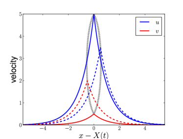
(a) (b)

Figure 3: Evolution of the velocity (Panel a) and momentum (Panel b) solutions of a coupled peakon pair.
Panel (a) shows the profile of velocity fields of a peakon-peakon couple with initial parameters $m_{0}=10$, $n_{0}=1$, $Y_{0}=0$ (solid lines). The dotted path indicates the evolution of the two peaks in the frame travelling at the particles’ mean velocity, $\dot{X}=\left(\dot{q}+\dot{r}\right)/2$. For these initial conditions, the total period of one orbit of the cycle is $T=3.6$. Also shown are the velocity fields at subsequent time intervals $t=0.45+1.8k$ for $k\in\mathbb{N}$ (dashed lines).
Panel (b) shows locus of the magnitude of momentum versus position for the two particles. The circles and crosses indicate the respective positions of each particle in phase space at time intervals of 1.44 units. The peakons are initially superposed at $x=0$, so that the leftmost circle and cross represent the same instant, and similarly for each couple continuing rightwards.
Animations showing the time evolution of both these images are available as supplementary material with the online copy of this paper.

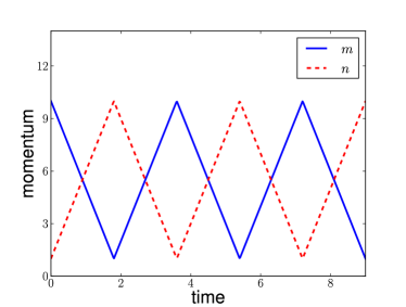
(a) (b)

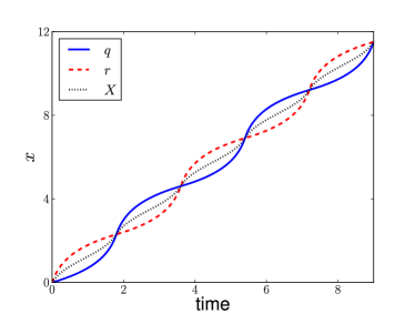
Figure 4: Plots of momentum (Panel a) and position (Panel b) versus time for the peakon-peakon couple with initial conditions $m_{0}=10$, $n_{0}=1$, $q_{0}=r_{0}=0$.
Panel (a) illustrates that, as per equation (41) the growth and decay of momenta are continuous and piecewise linear with respect to time in the interval between collisions, while the total momentum, $\mathcal{M}=m+n$, is conserved through collisions. Also shown is the discontinuity (and symmetry) in the first derivative of the momentum at the points of collision, which here occur every 1.8 time units.
Panel (b) illustrates the “waltzing” nature of the collision, with the identity of the leading particle alternating periodically, with the locus of the position of one particle obtainable from the other under a phase shift. Also plotted is the mean position $X=\left(q+r\right)/2$, showing the nonlinear relations in the propagation speed of the structure.

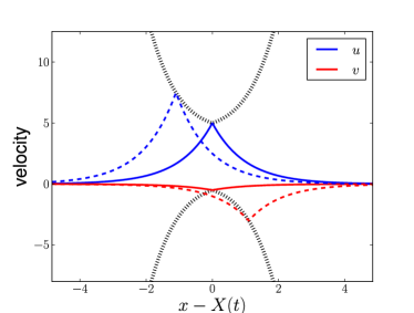
(a) (b)

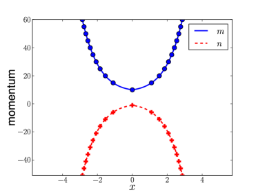
Figure 5: Evolution of the velocity (Panel a) and momentum (Panel b) solutions of a peakon-antipeakon coupled pair.
Panel (a) shows the velocity fields of anpeakon-antipeakon couple at time $t=0$ with $m_{0}=10$, $n_{0}=-1$, $Y_{0}=0$ (solid lines). The dotted path indicates the locus of the peaks, in the frame travelling at the mean particle velocity, $\dot{X}\left(t\right)=\left(\dot{q}+\dot{r}\right)/2$, as $t\rightarrow\pm\infty$. Also shown are the velocities at $t=1$.
Panel (b) shows the loci of the $(m,q)$ and $\left(n,r\right)$ particles in a stationary frame of reference centred on the point of collision. As in Figure 3, the dots and crosses indicated the particles location in phase space at regular time intervals. Here the best point of comparison is from $t=0$, when the particles are superposed at $q=r=0$.
Animations showing the time evolution of both these images are available as supplementary material with the online copy of this paper.

The final step is to consider the mean flow of the system. This is given by

$$\dot{X}=\left\{\begin{array}[]{cc}\frac{2\mathcal{M}E}{\mathcal{M}^{2}-\left[2Et-\overline{\mbox{sgn}}\left(Y_{0}\right)\left(n_{0}-m_{0}\right)\right]^{2}},&t<T_{0}\\ \frac{2\mathcal{M}E}{\mathcal{M}^{2}-\left[2E\left(t-T_{i}\right)-\sqrt{\mathcal{M}^{2}-8E}\right]^{2}}&T_{i}<t<T_{i+1}\end{array}\right.$$

i.e.

$$X-X_{0}=\left\{\begin{array}[]{cc}\left[\tanh^{-1}\left(\frac{2Et-\overline{\mbox{sgn}}\left(Y_{0}\right)\left(n_{0}+m_{0}\right)}{\mathcal{M}}\right)+\overline{\mbox{sgn}}\left(Y_{0}\right)\tanh^{-1}\left(\frac{n_{0}-m_{0}}{\mathcal{M}}\right)\right]&t<T_{0}\\ X\left(T_{i}\right)-X_{0}+\left[\tanh^{-1}\left(\frac{2E\left(t-T_{i}\right)-\sqrt{\mathcal{M}^{2}-8E}}{\mathcal{M}}\right)\right.\\ \qquad\qquad\qquad\qquad\qquad\qquad\left.+\tanh^{-1}\left(\frac{\sqrt{\mathcal{M}^{2}-8E}}{M}\right)\right]&T_{i}<t<T_{i+1}\end{array}.\right.$$

Figs. 3-5 illustrate this analytic solution in the both the peakon-peakon ($E>0$) and peakon-antipeakon ($E<0$) cases. Of particular interest in the peakon-peakon case is the nature of the collisions that occur. These collisions propagate the waltzing peakon couple onwards as a coherent phenomenon, possessing (in the tunnelling representation) continuous values for the particle positions, velocities and momenta, but with a discontinuous first derivative in the rate of change of momentum.

Note that over one entire cycle of the waltz, the mean speed of propagation is given by

$$\overline{\dot{X}}=\frac{1}{T_{i+1}-T_{i}}\int_{T_{i}}^{T_{i+1}}\dot{X}dt=\frac{m_{0}n_{0}}{2\left|m_{0}-n_{0}\right|}\tanh^{-1}\left(\frac{\left|m_{0}-n_{0}\right|}{m_{0}+n_{0}}\right).$$

Using l’Hospital’s rule we find that in the limit of zero period oscillations

$$\lim_{T_{0}\rightarrow 0}\overline{\dot{X}}=\lim_{m_{0}\rightarrow n_{0}}\frac{m_{0}^{2}}{2}\left(\frac{m_{0}+n_{0}-\left(m_{0}-n_{0}\right)}{\left(m_{0}+n_{0}\right)^{2}}\right)\left(\frac{1}{1-\left(\frac{m_{0}-n_{0}}{m_{0}+n_{0}}\right)^{2}}\right)=\frac{n_{0}}{2}.$$

This is exactly the velocity of a single peakon solution to the CH equations, to which the cross-coupled equations collapse under the same limit.

Triangular compacton couples.

Similarly, we may consider a compacton couple with a triangular kernel and corresponding Hamiltonian

$$H=\frac{1}{2}mn(1-a|q-r|)\theta(1-a|q-r|)$$ (43)

where $a$ is a constant. For initial conditions $q(0)=r(0)=0$, $n(0)=n_{0}$, $m(0)=m_{0}$, $n_{0}>m_{0}$ the solution is:

$$q(t)=\frac{m_{0}n_{0}}{2c}t+\frac{m_{0}^{2}}{ac^{2}}(1-e^{-cat/2}), r(t)=\frac{m_{0}n_{0}}{2c}t+\frac{n_{0}^{2}}{ac^{2}}(e^{cat/2}-1)$$

$$m(t)=\frac{cm_{0}}{m_{0}+n_{0}e^{-cat/2}}, n(t)=\frac{cn_{0}}{n_{0}+m_{0}e^{cat/2}}$$

Here $0\leq t\leq T_{1}=({4}/{ac})\ln{n_{0}}/{m_{0}}$ where $c=m_{0}+n_{0}$ is the conserved momentum. For the second half of the cycle the solution is

$$q(t)=K+\frac{m_{0}n_{0}}{2c}t+\frac{n_{0}^{2}}{ac^{2}}(e^{ca(t-T_{1})/2}-1)\,, r(t)=K+\frac{m_{0}n_{0}}{2c}t+\frac{m_{0}^{2}}{ac^{2}}(1-e^{-ca(t-T_{1})/2})\,,$$

$$m(t)=\frac{cn_{0}}{n_{0}+m_{0}e^{ca(t-T_{1})/2}}\,, n(t)=\frac{cm_{0}}{m_{0}+n_{0}e^{-ca(t-T_{1})/2}}\,,$$

for $T_{1}<t<2T_{1}$ and the constant $K=2\frac{m_{0}n_{0}}{ac^{2}}\ln\frac{n_{0}}{m_{0}}+\frac{n_{0}-m_{0}}{ac}$ represents the spatial shift during the first half cycle. The full cycle has a period $2T_{1}=\frac{8}{ac}\ln\frac{n_{0}}{m_{0}}$.

6 The Periodic Equilibrium Solutions

While the 1+1 soliton has only one equilibrium solution, with $m=n$ and $l=0$, the periodic solution has two. The first being the CH equivalent state with particles super-imposed, and the second with $m$ and $n$ multipeakons which are a half-step out of phase with each other. In such cases, the Greens function solution is given in the interval $-L\leq x<L$ by

$$m(x,t)=\sum_{a=1}^{M}m_{a}\left(t\right)\delta\left(x-q_{a}\left(t\right)\right),\qquad u(x,t)=\sum_{a=1}^{M}m_{a}\left(t\right)\frac{\cosh\left(L-|x-q_{a}\left(t\right)|\right)}{4\sinh L},$$

$$n(x,t)=\sum_{b=1}^{N}n_{b}\left(t\right)\delta\left(x-r_{b}\left(t\right)\right),\qquad v(x,t)=\sum_{b=1}^{N}n_{b}\left(t\right)\frac{\cosh\left(L-|x-r_{b}\left(t\right)|\right)}{4\sinh L},$$

and by the periodicity conditions, $m(x+2L)=m(x),\ n(x+2L)=n(x),$ etc., otherwise.

For the case $M=N=1$, upon dropping the indices $a$ and $b$ and defining once again

$$Y(x)=q(x)-r(x),$$

we see (eventually) that

$$\frac{d^{2}}{dt^{2}}2\tan^{-1}\left(\tanh\frac{L-|Y|}{2}\right)=-2E\,\mbox{sgn}^{2}\left(Y\right)\tanh\left(L-|Y|\right).$$

From this relation, we obtain the quadrature

$$\frac{d|Y|}{dt}=\left(\frac{1}{2}\ln\left(\cosh\left(L-|Y|\right)\right)+C\right)e^{-\frac{E\cosh\left(L-|Y|\right)}{\sinh\left(L\right)}},$$

where as before

$$E=\frac{m_{0}n_{0}}{2}e^{-|Y_{0}|},$$

and the constant of integration $C$ is found from the initial condition

$$\left.\frac{d|Y|}{dt}\right|_{t=0}=\mbox{sgn}\left(Y_{0}\right)\left(n_{0}-m_{0}\right)\frac{\cosh\left(L-|Y_{0}|\right)}{4\sinh L}\,.$$

7 The 2+2 Peakon-Antipeakon solution

We consider now the anti-symmetric collision of two couples of peakons in which, using the labelling pattern indicated in Figure 6 we have the following reduction of the system (36)–(39):

$$m_{1}=-m_{2}\equiv m,\quad n_{1}=-n_{2}\equiv n,\quad q_{1}=-q_{2}\equiv q,\quad r_{1}=-r_{2}\equiv r.$$

The reduced dynamical system in this case has the canonical Hamiltonian form,

$$\dot{q}=\frac{\partial H}{\partial m} = \frac{1}{2}n\left(e^{-|q-r|}-e^{-|q+r|}\right),$$

$$\dot{r}=\frac{\partial H}{\partial n} = \frac{1}{2}m\left(e^{-|q-r|}-e^{-|q+r|}\right),$$

$$\dot{m}=-\,\frac{\partial H}{\partial q} = \frac{1}{2}mn\left(\mbox{sgn}(q-r)e^{-|q-r|}-\mbox{sgn}(q+r)e^{-|q+r|}\right),$$

$$\dot{n}=-\,\frac{\partial H}{\partial r} = -\frac{1}{2}mn\left(\mbox{sgn}(q-r)e^{-|q-r|}+\mbox{sgn}(q+r)e^{-|q+r|}\right).$$

The Hamiltonian for this system is

$$H=\frac{1}{2}mn\left(e^{-|q-r|}-e^{-|q+r|}\right)$$

and its canonical Poisson bracket arises from the symplectic form $\omega=dq\wedge dm+dr\wedge dn$.

We choose to consider the colliding case

$$\mbox{sgn}\left(n\right)=\mbox{sgn}\left(m\right)>0$$

and

$$\mbox{sgn}\left(q\right)=\mbox{sgn}\left(r\right)<0.$$

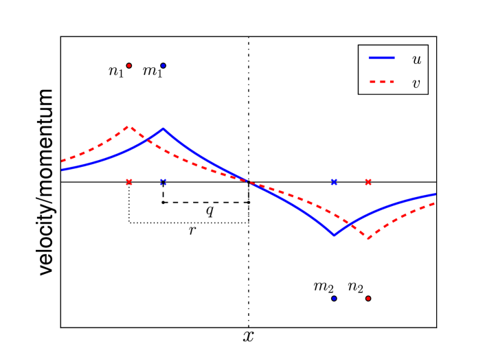
Figure 6: This is the head-on collision set-up used in our analysis. It has a rightward travelling peakon-peakon couple in the left half plane and an antisymmetric counterpart on the right. Each particle couple undergoes “waltzing” collisions before reaching, by symmetry, a singular collision at the point $x=0$.
An animation that shows the time evolution of such a peakon-antipeakon collision is available as supplementary material with the online copy of this paper.

Initially we suppose that $q(0)=r(0)=\ln k<0$ where from the energy conservation

$$k=\sqrt{1-\frac{2H}{m_{0}n_{0}}},$$

$m_{0}=m(0)$ and $n_{0}=n(0)$. Then we assume that $0>q(t)>r(t)$ until after some time $T$ again $q(T)=r(T)$ and another ’exchange’ of the positions of $n$ and $m$ takes place. Under these circumstances the system (7)–(7) for $0\leq t\leq T_{1}$ has the form

$$\dot{q}=-ne^{r}\sinh q\,,\quad\dot{r}=-me^{r}\sinh q\,,\quad\dot{m}=mne^{r}\cosh q\,,\quad\dot{n}=mne^{r}\sinh q$$

The system conserves the energy $H=-mne^{r}\sinh q$ and can be integrated, giving:

$$q(t)=\ln\left(\frac{(k+1)+(k-1)e^{-n_{0}kt}}{(k+1)-(k-1)e^{-n_{0}kt}}\right), r(t)=\ln\left(\frac{kn_{0}}{n_{0}-Ht}\right),$$ (44)

$$m(t)=H\frac{(k+1)^{2}-(k-1)^{2}e^{-2n_{0}kt}}{2kn_{0}(1-k^{2})e^{-n_{0}kt}}, n(t)=n_{0}-Ht.$$ (45)

The time to the next exchange, $T_{1}$ can be determined from $q(T_{1})=r(T_{1})$, i.e. from the equation

$$n_{0}-HT_{1}=kn_{0}\frac{(k+1)-(k-1)e^{-n_{0}kT_{1}}}{(k+1)+(k-1)e^{-n_{0}kT_{1}}}.$$ (46)

If $n_{0}>m_{0}$ this equation has a real root, which is less or equal to $n_{0}/H$. For $0<t<T_{1}$ $n(t)$ is decreasing and $m(t)$ is increasing.

The equations for the time following the exchange, i.e. when $0>r(t)>q(t)$ are

$$\dot{q}=-ne^{q}\sinh r, \dot{r}=-me^{q}\sinh r,$$

$$\dot{m}=mne^{q}\sinh r, \dot{n}=mne^{q}\cosh q.$$

with solutions

$$q(t)=\ln\left(\frac{k_{1}m_{1}}{m_{1}-H(t-T_{1})}\right), r(t)=\ln\left(\frac{(k_{1}+1)+(k_{1}-1)e^{-m_{1}k_{1}(t-T_{1})}}{(k_{1}+1)-(k_{1}-1)e^{-m_{1}k_{1}(t-T_{1})}}\right),$$

$$m(t)=m_{1}-H(t-T_{1}), n(t)=H\frac{(k_{1}+1)^{2}-(k_{1}-1)^{2}e^{-2m_{1}k_{1}(t-T_{1})}}{2km_{1}(1-k_{1}^{2})e^{-m_{1}k_{1}(t-T_{1})}},$$

where $m_{1}=m(T_{1})$, $n_{1}=n(T_{1})$ from (45) and (45) are the new (updated) initial conditions, and the updated value for the former constant $k$ is now

$$k_{1}=\sqrt{1-\frac{2H}{m_{1}n_{1}}}\,.$$

These solutions are valid until the time of the next collision, $T_{1}\leq t\leq T_{2}$ when again $q(T_{2})=r(T_{2})$ or, $T_{2}$ is a solution a similar transcendental equation:

$$m_{1}-H(T_{2}-T_{1})=k_{1}m_{1}\frac{(k_{1}+1)-(k_{1}-1)e^{-m_{1}k_{1}(T_{2}-T_{1})}}{(k_{1}+1)+(k_{1}-1)e^{-m_{1}k_{1}(T_{2}-T_{1})}},$$ (47)

The total time of the two exchanges, i.e. for a full cycle is $T=T_{2}$.

Thus the evolutionary process of the system that emerges from these solutions between the collisions is an iterative map illustrated in Figure 7.

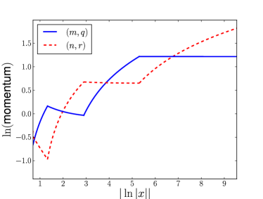
(a) (b)

Figure 7: Evolution of the momentum of the peakon couple in the anti-symmetric headon collision in terms of position (Panel a) and time (Panel b).
Panel (a) shows a log-log plot of momentum versus position for the peakon couple in the peakon-antipeakon collision, calculated from a numerical integration of the governing ODEs (7)-(7), (7)-(7). Here $m\left(0\right)=1,n\left(0\right)=2,q\left(0\right)=r\left(0\right)=-2$. This plot illustrates the evolution over two complete cycles of the ‘waltzing’ peakon, while also showing the near exponential increase in the momentum amplitudes over each full cycle.
Panel (b) shows momentum versus time for similar data, with $m\left(0\right)=1,n\left(0\right)=2,q\left(0\right)=r\left(0\right)=-3$. The last stage shows the rapid change from behaviour very similar to the pure peakon couple to near exponential growth as the particles in the peakon couple approach each other. In both cases the behaviour of the antipeakon couple is identical modulo a reversal of signature.

8 Other Collisions

We now present the results of numerical integration of the interaction between a peakon couple and other coherent structures. The numerical code solves the ODEs for the particle momenta and peak locations using an implicit midpoint rule integrator and a collision detection routine to identify the points of discontinuity in the momentum forcing term. This method can be used to investigate the short term behaviour of the ($M,N$) peakon equations for cases with $M$ and/or $N$ greater than one, for which we do not yet have an analytic description.

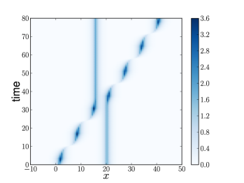
(a) (b)

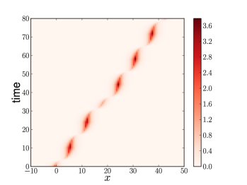
Figure 8: Spacetime plots showing an example of the evolution of the $u$ (panel a) and $v$ (panel b) velocity fields, under the interaction of a peakon couple with a free resting soliton. Here all particles are initially of momentum $m_{1}=m_{2}=n_{1}=4$, with initial positions $q_{1}=1$, $q_{2}=20$, $r_{1}=-1$. Comparison of the panels shows the beating amplitude and phase locking of the waltzing couple, which is interrupted when the $n$ particle interacts with the second $m$ particle.

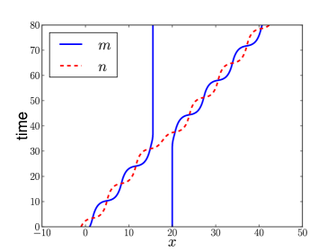
Figure 9: The space-time track of the particles presented in Figure 8. One waltzing partner deserts its old partner on interacting with another particle of opposite type, with a barely perceptible change in the period of oscillation (tempo) in the waltzing couple.
Animations that show the time evolution of this image and the underlying peakons are available as supplementary material with the online copy of this paper.

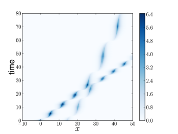
(a) (b)

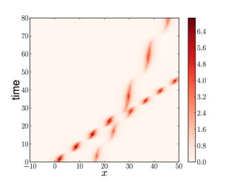
Figure 10: Spacetime plots showing an example of the evolution of the $u$ (Panel a) and $v$ (Panel b) velocity fields, under the interaction of two waltzing couples of peakons. Here $m_{1}=n_{1}=8$, $m_{2}=n_{2}=4$, $q_{1}=-1$, $q_{2}=14$, $r_{1}=1$, $r_{2}=16$. The peakon couples interact and exchange some momentum leading two a speeding up of the rightmost couple. However the collision also affects the “internal oscillation” energy of the two couples of particles, changing the period of oscillation of both constructs.

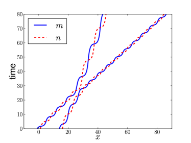
Figure 11: The space-time tracks of the waltzing couples of peakons from Figure 10. This makes it clearer that the two waltzing couples exchange momentum without ever actually overlapping, as well as illustrating the increased period of the lefthand couple and decreased period of the righthand one. Although not obvious, the post-exchange mean propagation speeds of the two couples also differ from those pre-collision.
Animations showing the time evolution of this image and the underlying peakons are available as supplementary material with the online copy of this paper.

8.1 Interaction between a peakon couple and a solitary peakon

This is the case with $M=2$, $N=1$, $\mbox{sgn}\left(m_{1}\right)=\mbox{sgn}\left(m_{2}\right)=\mbox{sgn}\left(n_{1}\right)$ in which a peakon couple interacts with a single peakon. The results of a typical integration are shown in Figs. 8-9, in terms of both the generated velocity fields and the tracks of the particles. Since the effect of one peakon on another falls exponentially with distance, a tightly bound peakon-peakon couple feels little influence from a distant solitary peakon, and by the same measure causes little change in the solitary peakon itself. However once the couple cycles sufficiently near at hand for the distance of the solitary peakon from the couple to be comparable to the maximum separation distance of the couple, the particle feels sufficient effect to be swept into motion. The ordering condition on the line is sufficient to guarantee that the formerly solitary particle is never overtaken by the other member of its type. In all integrations performed, the solitary peakon is swept up into a new waltzing couple, with the former partner abandoned, however we have no definite proof that there does not exist a parameter regime in which the three particles may form a coherent propagating structure.

8.2 Overtaking between two peakon couples

This is the case with $M=2$, $N=2$, $\mbox{sgn}\left(m_{a}\right)=\mbox{sgn}\left(n_{b}\right)$, in which two peakon couples interact. In general this requires the mean propagation speed of the trailing couple to be larger than that of the leading couple, so that the two structures interact in a manner equivalent to the CH overtaking collision. The results of a typical integration are shown in Figs. 10-11. As in the case of interaction with a solitary peakon, the particles behave in the manner of two pure cycling peakon-peakon couples, so long as the separation of the centres of the couples is significantly longer than the the maximum separation distance within either couple. Within the parameter space explored, the subsequent interaction is always at a distance, with no extra entanglement of the loops of the two tracks. The resulting exchange of momenta leads to an acceleration of the initially slower leading couple, with concomitant deceleration of the trailing couple. However, this exchange is not perfect, with additional energy partitioned into or out from the oscillatory motion, above that necessary to change the speed of progression. From the observed behaviour it can be conjectured that the long time solution of the ($n_{1}+n_{2}$,$n_{1}$) peakon cross-coupled equations for $n_{1},n_{2}\in\mathbb{N}$ is to form a chain of $n_{1}$ peakon-peakon couples, well ordered by their mean propagation speed, with $n_{2}$ near non propagating solitary peakons remaining. Due to the complex nature of propagation speed formula it is not, however possible to guarantee well ordering in either the momenta or the separation distances involved.

9 CCEP coupled compacton solutions

An arbitrary norm on the tangent space of vector fields, $\left\|u\right\|=\left(u,\mathcal{G}u\right),$ with $\mathcal{G}$ a symmetric operator on $u$ and its derivatives, induces cross-coupled equations through application of the CCCH framework to the new Lagrangian $l_{\mathcal{G}}\left(u,v\right)=\left(u,\mathcal{G}v\right).$ In particular, the convolutions $u=K_{\mathcal{G}}*m\quad\hbox{and}\quad v=K_{\mathcal{G}}*n,$ define the kernel $K_{\mathcal{G}}$ for the system, which inverts the momentum-velocity relation in the definitions of the momenta in the Legendre transformation,

$$m=\frac{\delta l_{\mathcal{G}}}{\delta v}\quad\hbox{and}\quad n=\frac{\delta l_{\mathcal{G}}}{\delta u}.$$

The numerical method, used in the previous section to integrate the Hamiltonian ODEs governing the peakon solutions of CCCH, was extended to solve the system of evolution equations for general Hamiltonians of the form

$$\frac{1}{2}H=\sum_{a,b=1}^{M,N}m_{a}(t)n_{b}(t)K_{\mathcal{G}}(|q_{a}-r_{a}|).$$ (48)

We consider in particular the two compactly supported kernels,

$$K_{1}(x)=\frac{1}{2}\left(1-\frac{x}{4}\right)\theta\left(1-\frac{x}{4}\right)\quad\hbox{and}\quad K_{2}(x)=\frac{1}{2}\left(1-\frac{x^{2}}{16}\right)\theta\left(1-\frac{x}{4}\right),$$ (49)

that are, respectively, triangular and parabolic. The profiles of these two compacton kernels are displayed in Figure 12, in comparison with the peakon profile, $\frac{1}{2}\exp(-|x|)$.

Much of the analysis of Section 5 generalises immediately to singular solutions of cross-coupled Euler-Poincaré (CCPE) equations with compacton kernels. When the centres of two solitary $m$ and $n$ particles lie within each other’s domains of support, the particles propagate together with the same form of cyclical motion for CCPE compactons as exhibited by the CCCH peakons. For example, numerical integrations shows the same results as for the peakon in the interaction of a cyclically propagating compacton couple with a solitary, stationary compacton, for each of the kernels, $K_{1}$ and $K_{2}$. These cases are essentially the same as in Figure 9 for identical initial particle weights and separations.

A new phenomenon for compacton collisions.

The collision problem for parabolic compaction couples with the $K_{2}$ profile does show an additional new property of the compacton systems. Namely, pair interactions may force the oscillations past the half-width of the compacton’s support, and thereby separate a waltzing compacton couple into two solitary compactons. The role of this phenomenon in multi-compacton interactions is explored in order of increasing complexity in Figs. (13), (14) and (17).

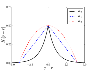
Figure 12: Plot shows the profile of the triangular and parabolic kernels, $K_{1}$ and $K_{2}$, defined in equations (49) and (49), as well as the CCCH peakon profile, $K_{0}$. The parabolic profile, $K_{2},$ has discontinuities in derivatives at $x=\pm 4$ but is smooth across the origin. The triangular profile, $K_{1}$, has discontinuities in its derivative at all three points, $x\in[-4,0,4]$.

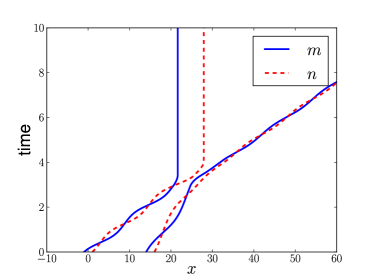
(a) (b)

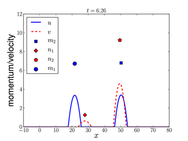
Figure 13: Panel (a) depicts spacetime plots for the pairwise overtaking problem equivalent to Figure 11, but with the parabolic compacton profiles in equation (49). The interaction is sufficiently violent that the trailing $n$ (blue) particle gains enough extra velocity to escape the region of support of its partner (red), breaking the cyclic red-blue couple into two stationary particles.
Panel (b) shows the positions and weights of the particles shortly after the collision, as well as the resultant velocity profiles. This clearly shows that the separation of the particles exceeds the compacton width.
This behaviour was also found for other compacton kernels (such as triangular compactons) in regimes with sufficiently energetic compacton couples. Overtaking collisions of cross-coupled compactons can thus influence the form of the long time solutions. This behaviour is not seen for systems of compacton equations that contain only a self interaction term.
Animations that show the time evolution of this image are available as supplementary material with the online copy of this paper.

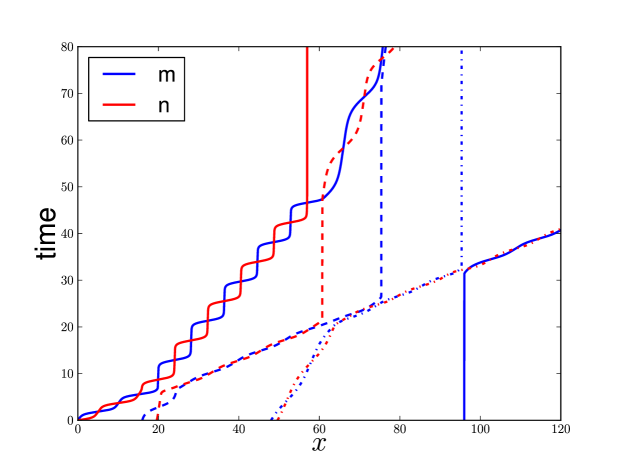
Figure 14: Spacetime paths for the problem of sequential pairwise overtaking collisions are plotted for three initially rightward-moving parabolic compacton couples, kernel $K_{2}$, arranged from left to right in order of decreasing propagation speed and one stationary parabolic compacton monopole. Initial conditions are given in form (species, weight, position) by $(m,8,0)$, $(n,0.8,0)$, $(m,1.6,8)$, $(n,1.6,9.8)$, $(m,0.8,24)$, $(n,0.8,24.8)$ and $(m,1.6,48)$. During the overtaking collisions, the left-right positional order is preserved separately for each species.
The first four collisions shown can be classified into three classes:

1. In the first collision, near $t=8$, $x=10$ the two colliding couples remain intact, but suffer sudden changes in their direction of propagation and in the periods of the cycles in both couples.

2. The second collision at $t=22$, $x=30$, involves the destruction of the faster (dashed) couple, resulting in two unbound monopoles, one of each species, the second of which (dashed blue) is ejected only after propagating for a few cycles as a compound state involving two blues ($m$) and one red ($n$). The collisions at later times all involve exchanges of partners.

3. The penultimate collision again involves formation of a compound state of two blues and one red. The compound state lasts for only two cycles in this case before the exchange is complete and the leftmost one (solid blue) is ejected.

4. The last collision involves the stationary monopole that was ejected in an earlier exchange collision. It exchanges again and propagates away in a couple. Thus, the initially rightmost positive compacton couples propagate away rightward.

Animations that show the time evolution of this image are available as supplementary material with the online copy of this paper.

10 Crossflow equations with more than two species

As a final example of the application of of this framework, we consider equations for multiple (i.e. more than two) species that cannot sustain motion without being in each other’s presence. For a vector of velocity vector fields, $\bm{u}=\left(u^{(1)},u^{(2)},\ldots,u^{(n)}\right)$, define a Lagrangian

$$l\left(\bm{u}\right)=\frac{1}{2}(\bm{u},\left(\bm{A}\right)\mathcal{G}\bm{u}),$$

with $\bm{A}$ a real symmetric matrix of determinant $\pm 1$, and $\mathcal{G}$ an arbitrary differential operator, applied elementwise. The resulting Euler-Poincaré equations are

$$\left(\frac{\partial}{\partial t}+\mathcal{L}_{u^{(i)}}\right)\frac{\delta l}{\delta u^{(i)}}=0,$$ (50)

for a vector of momenta, $\bm{m}:=\frac{\delta l}{\delta\bm{u}}=\bm{A}\mathcal{G}\bm{u}.$ The inversion of this Legendre transformation is

$$\bm{u}=\bm{A}^{-1}\left(K*\bm{m}\right)=K*\bm{A}^{-1}\bm{m},$$ (51)

where the convolution is also to be applied elementwise. The induced Hamiltonian for this system is thus

$$H=\frac{1}{2}\left(\bm{m},K*\bm{A}^{-1}\bm{m}\right),$$

with Hamiltonian motion equations

$$\partial_{t}\bm{m}+\left(\partial_{x}\bm{m}+\bm{m}\partial_{x}\right)\frac{\delta H}{\delta\bm{m}}=0.$$ (52)

An absence of self-interaction terms in the Lagrangian representation (50) requires that the matrix $\bm{A}$ have all entries on its leading diagonal vanish. This is the necessary and sufficient sufficient to ensure that no non-linear terms in a single species appear in the governing PDEs for the velocities, meaning initial conditions with non-vanishing velocity of a single species are steady.

Meanwhile, an absence of self interaction terms in the Hamiltonian representation (52) requires similarly that the inverse matrix $\bm{A}^{-1}$ have all the leading diagonal vanish, so that the the evolution of each element of $\bm{m}$ is instantaneously independent of its own value.

For $n=2$ the only matrix satisfying our conditions on symmetry, determinant and leading diagonal is

$$\bm{A}=\left(\begin{array}[]{cc}0&1\\ 1&0\end{array}\right),$$

which is unitary and generates generalizations of the CCCH. Thus, for this case of $n=2$ the CCCH are the canonical equations without self-interaction terms. For $n>2$ there may exist systems which are non-self interacting in only one of the two representations.

As a concrete example, consider the case for $n=3$ and Euler-Poincaré Lagrangian

$$l_{\mathrm{EP}}\left(u^{(1)},u^{(2)},u^{(3)}\right)=\frac{1}{4}\int\sum_{j\neq k=1}^{3}u^{(j)}u^{(k)}+u_{x}^{(j)}u_{x}^{(k)}dx,$$

i.e. the coupling matrix for the Euler-Poincaré case

$$[\bm{A}^{\mathrm{EP}}]_{ij}=\frac{1}{2}\left(1-\delta_{ij}\right)$$ (53)

has only cross-interaction terms. The choice of coupling matrix $[\bm{A}^{\mathrm{EP}}]$ gives momenta

$$m^{(1)}:=\frac{\delta l_{\mathrm{EP}}}{\delta u^{(1)}}=\left(1-\frac{\partial^{2}}{\partial x^{2}}\right)\left[\frac{u^{(2)}+u^{(3)}}{2}\right]$$ (54)

and cyclic permutations of 1,2,3. The velocities then relate to the momenta by

$$u^{(1)}=K*\left[m^{(2)}+m^{(3)}-m^{(1)}\right],$$ (55)

and cyclic permutations of the labels 1,2,3. The EP multi-species cross-coupled system has Hamiltonian

$$H_{\mathrm{EP}}=\frac{1}{2}\int\sum_{j\neq k=1}^{3}m^{(j)}K*m^{(k)}-\sum_{j=1}^{3}m^{(j)}K*m^{(j)}dx,$$ (56)

in which the last term involves self-interaction.

Another, complementary, cross-coupled system exists, in which the Hamiltonian representation has no self-interaction terms. This complementary cross-coupled system is a Lie-Poisson Hamiltonian system generated by

$$H_{\mathrm{LP}}=\frac{1}{2}\int\sum_{j\neq k=1}^{3}m^{(j)}K*m^{(k)}dx$$ (57)

with velocities given by, cf. equation (55),

$$u^{(1)}=K*\left[\frac{m^{(2)}+m^{(3)}}{2}\right]$$ (58)

and cyclic permutations of the labels 1,2,3. This formula implies the following Lagrangian for the LP multi-species cross-coupled system,

$$l_{\mathrm{LP}}\left(u^{(1)},u^{(2)},u^{(3)}\right)=\frac{1}{4}\int\sum_{j\neq k=1}^{3}\left[u^{(j)}u^{(k)}+u_{x}^{(j)}u_{x}^{(k)}\right]-\sum_{j=1}^{3}\left[\left(u^{(j)}\right)^{2}+\left(u_{x}^{(j)}\right)^{2}\right]dx$$

and thus a different coupling matrix from (53), namely,

$$[\bm{A}^{\mathrm{LP}}]_{ij}=\left[\bm{A}_{\mathrm{EP}}^{-1}\right]_{ij}=(1-2\delta_{ij})$$ (59)

Figures 15–16 show the results of integrating the singular solutions of these two different equation sets for the same initial conditions (in momentum space). The two equation sets have markedly different behaviour because of their differences in interactions. In particular, the self-interaction term in the EP Hamiltonian (56) induces a leftward drift for positively weighted particles and thereby allows for complexly coupled three-way interactions. In contrast, the three-species problem for the LP cross-coupled equations has fewer differences from CCCH for two species.

As more species are added, the scope for more complex interesting interactions grows. For example, Figure 17 shows the result of a run with parabolic compactons of twelve separate species in the relevant Hamiltonian cross-flow system. This shows both the complex entanglement of the various particles and the trivial classicifaction of many interaction features into those already described in the two species compacton case.

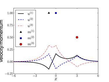
(a) (b)

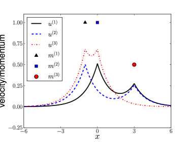
Figure 15: Initial conditions for three species cross-coupled equations in the Lagrangian (Panel a) and Hamiltonian representations (Panel b). In each case the locations and weights of the momentum particles, $m^{(i)}$, are identical. However, the resultant velocity fields, $u^{(i)}$, which carry each of the particles differ markedly. Comparision of the panels shows the impact of the strong negative self-interaction term in the viscinity of each particle in the Lagrangian representation.

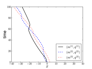
(a) (b)

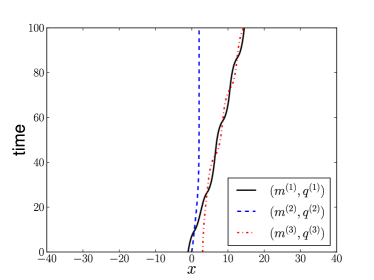
Figure 16: Spacetime plots for three species cross-coupled equations in the Lagrangian (Panel a) and Hamiltonian representations (Panel b) with the initial conditions shown in Figure 15.
Panel (a) shows the great significance of the negative momentum self-interaction term which appears in equation (54). All particles experience a leftward drift, proportional to their own magnitude. Moreover the fully coupled nature of the momentum equations allows.
The Hamiltonian representation in Panel (b) behaves much more in the manner of the CCCH solutions. In fact for these initial conditions the solution is very similar to one in which the $m^{(2)}$ and $m^{(3)}$ particles are of the same species.

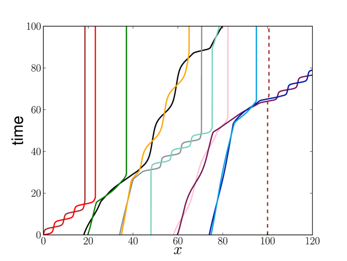
Figure 17: A space-time plot is shown of the evolution starting from initial conditions consisting of 12 separate species in the LP cross-coupled representation, whose Hamiltonian, as in (57), has no self-interaction terms. The initial conditions are chosen to form five parabolic compacton couples and two single parabolic compactons. All of the compactons are positive, so all of the couples propagate rightward. The same three basic forms of collision appear as in the previous figures for the CCCH equations however the particles no longer discriminate in their exchange of partners. The final space-time plot is reminiscent of the map of the London Underground!
Animations that show the time evolution of this image are available as supplementary material with the online copy of this paper.

The primary stable features for the multi-species collisions in Figure 17 are the same as for two species collisions in Figure 14, in that both include solitary particles and waltzing pairs. However, the transient collision behaviour in the multi-species case can be significantly more complex, possessing, for example, fully entangled three-way collisions, particle tunnelling and “hop-scotch”, in which a solitary particle is bled of its momentum by a coupled pair, then abandoned.

11 Conclusions/Discussion

Explicit outstanding problems.

Several outstanding problems were identified explicitly in the course of this work. These include the following tasks.

1. Study and classify the full set of interactions of the peakons in (20) for the CCCH system (31). Determine whether the generalizations proposed in systems (31) are integrable, or even whether the (weak) solutions exist and are unique.

   Even if the CCCH equations are not completely integrable, the generalisation they represent is interesting for its singular solutions and geometrical interpretation. In this regard, we may remark about additional symmetry and complete integrability of the corresponding coupled rigid body dynamics. Namely, if the problem specified here for a right-invariant Lagrangian on $\mathfrak{X}(\mathbb{R})\times\mathfrak{X}(\mathbb{R})$ had been expressed instead on $\mathfrak{so}(3)\times\mathfrak{so}(3)$ for a left-invariant Lagrangian, the result would have been interpretable as the dynamics of a cross-coupled system of two rigid bodies. This dynamics would have been expressible in Lie-Poisson form and it would have been completely integrable as a Hamiltonian system, only provided an additional $SO(2)$ symmetry were present, as for the case of axisymmetric coupled rigid bodies. In the present case, there seems to be no extra symmetry that would make the corresponding CCCH Hamiltonian system (31) completely integrable.

2. Explore the dynamical systems properties of the $(M,N)$-peakon solutions (20) of the CCCH equations (31). For example, determine the results of colliding a compacton couple with a single compacton of opposite sign.

3. Characterise the creation of peakons and peakon couples as a process of blow-up in finite time. We have sought an analog of the steepening lemma for the CH equation in [2] to explain how peakon couples arise from smooth initial conditions for the CCCH equations, but so far this result has eluded us.

4. Discuss the solution behaviour of other cross-coupled equations, such as cross-coupled Burgers (CCB), cross-coupled Korteweg de Vries (CCKdV) and cross-coupled $b$-equations. This is a wide open problem.

References

- [1] Acheson, D. J. Elementary Fluid Dynamics. Oxford University Press (Oxford, 1990).
- [2] Camassa, R. and Holm, D. D. An integrable shallow water equation with peaked solitons. Phys. Rev. Lett. 71 (1993) 1661–1664.
- [3] Camassa, R., Holm, D. and Hyman, J. A new integrable shallow water equation. Adv. Appl. Mech. 31 (1994) 1–33.
- [4] Chen M., Liu S.-Q. and Zhang Y. A two-component generalization of the Camassa-Holm equation and its solutions. Lett. Math. Phys. 75 (2006) 1–15; nlin.SI/0501028.
- [5] Constantin, A. and Lannes, D. The hydrodynamical relevance of the Camassa-Holm and Degasperis-Procesi equations. Arch. Rat. Mech. Anal. 192 (2009) 165–186.
- [6] Constantin, A. and Ivanov, R.I. On an integrable two-component Camassa-Holm shallow water system. Phys. Lett. A 372 (2008) 7129–7132.
- [7] Dai, H.-H. Model equations for nonlinear dispersive waves in a compressible Mooney-Rivlin rod. Acta Mech. 127 (1998) 193–207.
- [8] Dullin H. R., Gottwald G. A. Holm D. D., Camassa-Holm, Korteweg-de Vries-5 and other asymptotically equivalent equations for shallow water waves, Fluid Dynam. Res. 33 (2003) 73–95.
- [9] Dullin H. R., Gottwald G. A. Holm D. D. On asymptotically equivalent shallow water wave equations, Physica 190D (2004) 1–14.
- [10] Escher J., Lechtenfeld O. and Yin, Z. Well-posedness and blow-up phenomena for the 2-component Camassa-Holm equation. Discrete Contin. Dyn. Syst. 19 (2007) 493–513.
- [11] Holm D.D. Peakons, in Encyclopedia of Mathematical Physics, eds. J.-P. Françoise, G.L. Naber and Tsou S.T. Oxford Elsevier, 2006 (ISBN 978-0-1251-2666-3), volume 4 pages 12–20.
- [12] Holm D. D. and Ivanov R. I., Smooth and peaked solitons of the CH equation, J. Phys A Math. and Theor. 43 (2010) 434003 (18pp).
- [13] Holm D. D. and Ivanov R. I., Two-component CH system: Inverse Scattering, Peakons and Geometry, Inv. Problems, (2011), to appear, arXiv:1009.5374v1 [nlin.SI]
- [14] Holm D. D. and Ivanov R. I., Multi-component generalizations of the CH equation: geometrical aspects, peakons and numerical examples, J. Phys. A: Math. Theor. 43 (2010) 492001 (20pp).
- [15] Holm, D. D. and J. E. Marsden [2004], Momentum maps and measure-valued solutions (peakons, filaments and sheets) for the EPDiff equation, in The Breadth of Symplectic and Poisson Geometry, A Festshrift for Alan Weinstein, 203-235, Progr. Math., 232, J. E. Marsden and T. S. Ratiu, Editors, Birkhäuser Boston, Boston, MA, 2004.
- [16] Holm, D. D., Marsden, J. E. and Ratiu, T. S. The Euler-Poincaré equations and semidirect products with applications to continuum theories. Advances in Mathematics, 137(1):1–81, 1998.
- [17] Holm D. D., Ó Náraigh, L. and Tronci, C. Singular solutions of a modified two-component CH equation. Phys. Rev. E (3) 79 (2009) no. 1, 016601, 13 pp.
- [18] Holm D. D., Schmah, T. and Stoica, C. Geometric mechanics and symmetry. From finite to infinite dimensions. With solutions to selected exercises by D. C. P. Ellis. Oxford Texts in Applied and Engineering Mathematics, 12. Oxford University Press, Oxford, 2009.
- [19] Ivanov R. I. Extended CH hierarchy and conserved quantities, Z. Naturforsch., 61a (2006) pp. 133–138; nlin.SI/0601066.
- [20] Ivanov, R. I. Two-component integrable systems modelling shallow water waves: the constant vorticity case. Wave Motion 46 (2009) 389–396.
- [21] Johnson, R. S., Camassa-Holm, Korteweg-de Vries and related models for water waves. J. Fluid. Mech. 455 (2002) 63–82.
- [22] Johnson, R. S. The CH equation for water waves moving over a shear flow. Fluid Dynamics Research 33 (2003) 97–111.
- [23] Olver, P. and Rosenau, P. Tri-Hamiltonian duality between solitons and solitary-wave solutions having compact support. Phys. Rev. E (3) 53 (1996) 1900–1906.
- [24] Rosenau, P. and Hyman, J. M. Compactons: Solitons with finite wavelength Phys. Rev. Lett. 70 (1993) 564–567.