Deterministic Bounds for Restricted Isometry
of Compressed Sensing Matrices

Abstract

Compressed Sensing (CS) is an emerging field that enables reconstruction of a sparse signal $x\in{\mathbb{R}}^{n}$ that has only $k\ll n$ non-zero coefficients from a small number $m\ll n$ of linear projections. The projections are obtained by multiplying $x$ by a matrix $\Phi\in{\mathbb{R}}^{m\times n}$ — called a CS matrix — where $k<m\ll n$. In this work, we ask the following question: given the triplet $\{k,m,n\}$ that defines the CS problem size, what are the deterministic limits on the performance of the best CS matrix in ${\mathbb{R}}^{m\times n}$? We select Restricted Isometry as the performance metric. We derive two deterministic converse bounds and one deterministic achievable bound on the Restricted Isometry for matrices in ${\mathbb{R}}^{m\times n}$ in terms of $n$, $m$ and $k$. The first converse bound (structural bound) is derived by exploiting the intricate relationships between the singular values of sub-matrices and the complete matrix. The second converse bound (packing bound) and the achievable bound (covering bound) are derived by recognizing the equivalence of CS matrices to codes on Grassmannian spaces. Simulations reveal that random Gaussian $\Phi$ provide far from optimal performance. The derivation of the three bounds offers several new geometric insights that relate optimal CS matrices to equi-angular tight frames, the Welch bound, codes on Grassmannian spaces, and the Generalized Pythagorean Theorem (GPT).

I Introduction

I-A Compressed Sensing

Many signal processing applications focus on identifying and estimating a few significant coefficients from a high dimension vector. The wisdom behind this approach is the ubiquitous compressibility of signals: most of the information contained in a signal often resides in just a few large coefficients. Traditional sensing, compression and processing systems first acquire the entire data, apply a transformation to the data, and then discard most of the coefficients; we retain only a small number of significant coefficients. Clearly, it is wasteful to sense and compute on all of the coefficients when most coefficients will be discarded at a later stage. This naturally begs the question: can we sense compressible signals in a compressible way? In other words, can we sense only that portion of the signal that will not be thrown away? The ground-breaking work of compressed sensing (CS) pioneered by Candés et al. [1] and Donoho [2] answers this question in the affirmative.

Candés et al. [1] and Donoho [2] have demonstrated that the information contained in the few significant coefficients can be captured (encoded) by a small number of random linear projections. The original signal can then be reconstructed (decoded) from these random projections using an appropriate decoding scheme. Consider a discrete-time signal $x\in{\mathbb{R}}^{n}$ that has only $k\ll n$ non-zero coefficients. CS posits that it is unnecessary to measure all the $n$ values of $x$; rather, we can recover $x$ from a small number of projections onto an incoherent basis [1, 2]. To measure (encode) $x$, we compute the measurement vector $y\in{\mathbb{R}}^{m}$ containing $m$ linear projections of $x$ via the matrix-vector multiplication $y=\Phi x$, where $\Phi\in{\mathbb{R}}^{m\times n}$ is the CS matrix. The CS theory asserts that we can reconstruct (decode) $x$ given $y$ and $\Phi$ using $m\ll n$ measurements, provided certain requirements on $\Phi$ are satisfied.

It can be shown that if the CS matrix $\Phi$ is constructed by filling its $m\times n$ entries randomly from an i.i.d. Gaussian distribution, then with probability one, $m=k+1$ measurements are sufficient to encode $x$. In particular, with probability one, $x$ can be reconstructed exactly from $y\in{\mathbb{R}}^{m}$, $m\geq k+1$, using $\ell_{0}$ minimization [3]:

$$\min_{x\in{\mathbb{R}}^{n}}\|x\|_{0}\mbox{ subject to }\Phi x=y,$$ (1)

where $\|x\|_{0}=\{\#x_{i}:x_{i}\neq 0\}$. However, signal recovery algorithms using as few as $m=k+1$ measurements require a search in each of the ${n\choose k}$ subspaces that could contain the significant signal coefficients. Consequently the complexity of the algorithm to recover $x$ using (1) is NP complete [4]. Fortunately, at the expense of acquiring slightly more measurements, we can recover $x$ from $y$ thru a convex relaxation of (1); the complexity of the resulting recovery algorithm can be made polynomial. With $m\approx k\log(n/k)$ measurements, the solution to the $\ell_{1}$ minimization (which can be solved with cubic complexity) given by

$$\min_{x\in{\mathbb{R}}^{n}}\|x\|_{1}\mbox{ subject to }\Phi x=y,$$ (2)

coincides with the solution of (1) for $\Phi$ constructed from i.i.d. Gaussian distribution [1, 2]. The ability to recover sparse signals easily (in polynomial time) from the small number of CS measurements is one of the main reasons why CS has enjoyed tremendous attention in the research community over the last few years [5].

I-B What is a Good Compressed Sensing Matrix?

The CS matrix $\Phi$ plays a vital role in both data acquisition and the subsequent recovery of sparse signals. Not only do the properties of $\Phi$ dictate how much information we capture about the signal $x$, but they also determines the ease of reconstructing $x$ from the measurements $y$. In this paper, we select Restricted Isometry as proposed by Candés and Tao [6] as the metric to determine whether a given $\Phi$ is a good candidate for CS data acquisition. The reason we choose this metric is because several key results in CS depend on the Restricted Isometry properties of $\Phi$ [6, 1, 7, 8, 9, 10, 11, 12, 13, 14, 15, 16, 17, 18].

I-C Restricted Isometry Property

Definition 1

For each integer $k=1,2,...$, define the Restricted Isometry constant $\delta_{k}$ of a matrix $\Phi\in{\mathbb{R}}^{m\times n}$ as the smallest number such that

$$(1-\delta_{k})\|x\|_{\ell_{2}}^{2}\leq\|\Phi x\|_{\ell_{2}}^{2}\leq(1+\delta_{k})\|x\|_{\ell_{2}}^{2}$$ (3)

holds for all non-zero vectors $x\in{\mathbb{R}}^{n}$ that satisfy $0<\|x\|_{0}\leq k$.

Note that a “good” CS matrix has a small Restricted Isometry constant $\delta_{k}$.

As noted before, a number of key results in CS involve the Restricted Isometry constant. We highlight two results, both taken from [18]. Theorem 1 shows that if the Restricted Isometry constant $\delta_{2k}$ of order $2k$ is sufficiently small, then CS recovery is guaranteed to be tractable. Theorem 2 shows that the same condition on $\delta_{2k}$ guarantees robustness in CS recovery when the measurements are corrupted with bounded additive noise.

For Theorems 1 and 2, we assume $x$ is any signal in ${\mathbb{R}}^{n}$ and not necessarily $k$-sparse. Let $x_{k}\in{\mathbb{R}}^{n}$ be the best $k$-term approximation of $x$, ie, $x_{k}$ is obtained by taking $x$ and setting all but the $k$ largest magnitude entries to zero. Note that if $x$ is $k$-sparse, then $x=x_{k}$.

Theorem 1

[18, Theorem 1.1, page 2] If $\delta_{2k}$ satisfies $\delta_{2k}<\sqrt{2}-1$, then the solution $x^{*}$ to the $\ell_{1}$ minimization (2) obeys

$$\|x^{*}-x\|_{\ell_{1}}\leq C_{0}\|x-x_{k}\|_{\ell_{1}},$$ (4)

and

$$\|x^{*}-x\|_{\ell_{2}}\leq C_{0}k^{-1/2}\|x-x_{k}\|_{\ell_{1}}$$ (5)

for some constant $C_{0}$. In particular, if $x$ is $k$-sparse, then the recovery is exact.

Theorem 1 asserts that the solution of the $\ell_{1}$ minimization is exact when $x$ is $k$-sparse and when $\delta_{2k}$ is sufficiently small. Rather than solving the intractable $\ell_{0}$ minimization of (1) directly, we obtain the same solution using the tractable $\ell_{1}$ minimization as given by (2). Note that with only $m=k+1$ measurements, the CS matrix cannot satisfy the condition on $\delta_{2k}$. However, with more measurements and with specific construction of CS matrices (which can be either deterministic or stochastic), it can be shown that the condition in Theorem 1 can be satisfied surely or with high probability [2, 1, 7, 9].

The same upper-bound on $\delta_{2k}$ serves as a sufficient condition for the recovery to be robust in the presence of bounded additive noise. Consider noisy measurements

$$y=\Phi x+z,$$ (6)

where $z$ is an unknown noise vector that is bounded $\|z\|_{\ell_{2}}\leq\epsilon$. Consider the convex optimization problem

$$\min_{x\in{\mathbb{R}}^{n}}\|x\|_{\ell_{1}}\mbox{ subject to }\|y-\Phi x\|_{\ell_{2}}\leq\epsilon.$$ (7)

The following Theorem shows that sufficiently small Restricted Isometry constant $\delta_{2k}$ guarantees robust CS recovery of $k$-sparse signals in the presence of bounded measurement noise. Specifically, if the noise is bounded, then the error in signal recovery is also bounded.

Theorem 2

[18, Theorem 1.2, page 3] If $\delta_{2k}<\sqrt{2}-1$ and $\|z\|_{\ell_{2}}\leq\epsilon$, then the solution $x^{*}$ to the optimization (7) obeys

$$\|x^{*}-x\|_{\ell_{2}}\leq C_{0}k^{-1/2}\|x-x_{k}\|_{\ell_{1}}+C_{1}\epsilon$$ (8)

with the same constant $C_{0}$ as in Theorem 1 and some fixed $C_{1}$. In particular, if $x$ is $k$-sparse, then $\|x^{*}-x\|_{\ell_{2}}\leq C_{1}\epsilon$.

The central role played by the Restricted Isometry in CS begs the question: what is the best (smallest) Restricted Isometry constant we can hope to attain for a CS matrix in ${\mathbb{R}}^{m\times n}$ for a given triplet $n$, $m$ and $k$? This key question is what we investigate in this paper.

I-D Notations and Definitions

We define CS problem size as the triad of numbers $\{n,m,k\}$. For a fixed problem size, the CS matrix $\Phi$ is chosen from ${\mathbb{R}}^{m\times n}$. As we shall see shortly, the Restricted Isometry of $\Phi$ depends on the singular values of the $m\times k$-sized submatrices of $\Phi$ (which are ${n\choose k}$ in number.) While we focus mainly on real valued $\Phi$, several of the results we derive hold for complex valued $\Phi$ as well; we will explicitly mention if the results are applicable in the complex domain.

We exploit the fact that the measurements $y$ depend only on $k$ out of the $n$ columns of $\Phi$ when $x$ is $k$-sparse; the $k$ columns are the ones that correspond to the indices of the non-zero entries in $x$. As a consequence, the Restricted Isometry constant depends directly on the properties of the $m\times k$ sized submatrices of $\Phi$. This observation motivates us to consider the singular values of submatrices $\Phi_{p}\in{\mathbb{R}}^{m\times k}$ formed by selecting only $k$ of the $n$ columns of $\Phi$. The index $p\in[1,2,...,{n\choose k}]$ uniquely identifies the set of columns chosen from the complete matrix $\Phi$. Let the singular values of the matrix $\Phi$ be $S_{1}$, $S_{2}$,…, $S_{m}$, where $S_{1}\geq S_{2}\geq...\geq S_{m}\geq 0$. Furthermore, let the singular values of the submatrix $\Phi_{p}$ be $s_{p,1}$, $s_{p,2}$,…, $s_{p,k}$, where $s_{p,1}\geq s_{p,2}\geq...\geq s_{p,k}\geq 0$.

We define $\rho_{\max}(\Phi,k)\geq 0$ and $\rho_{\min}(\Phi,k)\geq 0$, respectively, as the maximum and the minimum of the singular values of every submatrix of $\Phi$ of size $m\times k$, that is,

$$\rho_{\max}(\Phi,k)=(\max_{p}\{s_{p,1}\})^{2}\mbox{ ~{}~{}~{}~{}~{} and ~{}~{}~{}~{}~{}}\rho_{\min}(\Phi,k)=(\min_{p}\{s_{p,k}\})^{2}.$$ (9)

Clearly, for a $k$-sparse signal $x$, we have that

$$\rho_{\min}(\Phi,k)\|x\|_{\ell_{2}}^{2}\leq\|\Phi x\|_{\ell_{2}}^{2}\leq\rho_{\max}(\Phi,k)\|x\|_{\ell_{2}}^{2},$$ (10)

where both inequalities in the above equation are tight. We define the Restricted Isometry Property Ratio (RIP ratio) as

$$R(\Phi,k)=\frac{\rho_{\max}(\Phi,k)}{\rho_{\min}(\Phi,k)}.$$ (11)

This ratio plays the role of the square of the condition number of $\Phi$ when it is applied exclusively to the domain of $k$-sparse signals.

We denote the differential operator $\frac{d}{dx}$ by $D$, i.e., $D[f(x)]=\frac{d}{dx}f(x)$, $D^{2}[f(x)]=\frac{d^{2}}{dx^{2}}f(x)$ and so on. We use the same variable name $x$ when we consider polynomials such as the characteristic equations of $\Phi$ and its submatrices. Any ambiguity with reference to our $k$-sparse signal $x$ is resolved from the context in which it is presented.

I-E Contributions

Existing results on Restricted Isometry in the CS literature provide achievability results on specific constructions of $\Phi$ (such as random i.i.d. Gaussian) [1, 2, 7, 9]. Most of the results are stochastic, along the lines of: “constructing a matrix according to a prescribed method (such as populating the matrix with i.i.d. Gaussian or i.i.d. Bernoulli entries) yields a CS matrix that satisfies RIP with a given $\delta_{k}$ with high probability [7]”. There have also been recent results on deterministic achievability, where a deterministic construction of $\Phi$ is proved to satisfy a statistical RIP (more on statistical RIP in Section V) for some constant $\delta_{k}$ [9].

Optimal CS reconstruction is intimately related to Gelfand and Kolmogrov widths of $\ell_{p}$ balls, an area that was extensively studied in the late 1970’s and early 1980’s by Kashin, Gluskin, and Garnaev [19, 20, 21, 22, 23]. Connections between the two fields have been recognized by Donoho [2] and others [24, 25, 7, 26] and have led to several deterministic bounds on Restricted Isometry. However, these prior results offer little insight into the structure of CS matrices that are optimal in the Restricted Isometry sense. In this work, we fill this gap by revealing the intricate relationships between optimal CS matrices and several well known results in coding theory and frame theory. As an important consequence of our work, we stumble upon a result that extends the well-known Welch bound [29] to higher orders.

In this paper, we derive two deterministic converse bounds for the RIP ratio based respectively on the structural properties of the CS matrix and packing of subspaces in ${\mathbb{R}}^{m\times n}$. Additionally, we also derive a deterministic achievable bound for the RIP ratio, which says that we can certainly find a $\Phi\in{\mathbb{R}}^{m\times n}$ that has a better RIP ratio than our new achievable bound.

The first bound we derive is a deterministic converse bound on the RIP ratio, called the structural bound. It is a function of the problem size $\{n,m,k\}$. The key insight that we use to derive it is that the singular values $\{s_{p,i}\}$ of $\Phi_{p}$ (submatrices of $\Phi$) are severely constrained by the singular values $\{S_{j}\}$ of the complete matrix $\Phi$. For example, the interlacing inequality [27] requires that

$$s_{p,i}\leq S_{i}\mbox{ for all }i=1,2,...,k,$$

and therefore the $\{s_{p,i}\}$’s cannot take on arbitrary values. We explore the intricate relationships between the two sets $\{s_{p,i}\}$ and $\{S_{i}\}$ of singular values to derive the structural bound on the RIP ratio. The structural bound places a limit on the best (smallest) RIP ratio that is attainable for matrices in ${\mathbb{R}}^{m\times n}$. Theorem 4 in Section II is the main result on this bound. The Theorem holds not only for real valued $\Phi$, but also for complex valued $\Phi$. We also show how the structural bound is related to equi-angular tight frames (ETF) [28], Welch bound [29], and the the Generalized Pythagorean Theorem [30, 31].

The second bound is also a deterministic converse bound on the RIP, called the packing bound. It is applicable to real-valued $\Phi$. In this paper, we derive the packing bound for the limited case of $k=2$; however, we plan to extend the results for $k>2$ in a future paper. The need for the packing bound is motivated by the fact that the structural bound is loose for large values of $n$ (in comparison to $m$ and $k$); the packing bound offers a tighter bound in the regime of large $n$. The packing bound is derived from an entirely different perspective: we consider the $n$ columns of $\Phi$ as vectors in ${\mathbb{R}}^{m}$ and show that minimizing the RIP ratio is equivalent to finding $n$ vectors in ${\mathbb{R}}^{m}$ where the angular separation of every pair of vectors is as large as possible. In other words, we show that deriving the optimal RIP ratio for $k=2$ is equivalent to optimal packing in Grassmannian spaces. The main result of the packing bound is presented in Theorem 5 in Section II.

The two converse bounds are applicable to every matrix in ${\mathbb{R}}^{m\times n}$. Therefore, the results provide bounds on the best (smallest) possible RIP ratio that any CS matrix can achieve for a given problem size. We also discuss which of the two converse bounds presented is likely to be the tighter bound, based on the particular selection of $\{k,m,n\}$.

The third bound we derive is a deterministic achievable bound, called the covering bound, which also exploits the equivalence of CS matrices to packing in a grasmannian space. We use a Theorem derived independently by Chabauty, Shannon, and Wyner [32, 33, 34] that uses covering arguments in order to guarantee achievability. The result is of the following flavor: there exists at least one $\Phi$ in ${\mathbb{R}}^{m\times n}$ that has RIP ratio equal to or better (smaller) than the one given by the covering bound. The main result of this bound is Theorem 6 in Section II. Again, our derivation considers only the case $k=2$; we plan to extend the results for $k>2$ in a future publication.

After deriving the bounds, we present extensive numerical results from which we draw several important observations and conclusions.

A summary of our key results made visual in the Figures is given below:

1. We see from Figure 1 that there is a large gap between the RIP ratio of Gaussian matrices and the achievable bounds. This observation points to the existence of CS matrices that are far superior than Gaussian matrices in terms of the RIP ratio.

2. We see from Figure 1 that, for small values of $n$, the structural bound is the tighter of the two converse bounds, whereas for large values of $n$, the packing bound is tighter.

3. Figure 1 also presents a graphical illustration of all three bounds and compares the bounds to the RIP ratio of Gaussian matrices, as well as the best known matrix for the given problem size. We use the results of Conway, Hardin, and Sloane [35, 36, 37], who have run extensive computer simulations to extract the best known packings in Grassmannian spaces.

4. While the structural bound for the RIP ratio has been derived for any $n$, $m$, and $k$, we presently have the packing and covering bounds only for $k=2$. Figure 2 depicts the structural bound for $k=4$ and $k=10$.

5. Figure 3 shows how the parameters of the structural bound can shed light on the statistical RIP that was proposed recently [38, 39, 9, 8]. In particular, we demonstrate a way to estimate the singular values of a randomly chosen submatrix of $\Phi$ in Section V.

Furthermore, we show that the structural bound for $k=2$ is equivalent to the Welch bound [29]. The structural bound for $k>3$ can be thought of as extensions to the Welch bound to higher orders $k>2$. We state our extension to the Welch bound explicitly in Theorem 70.

The results we present offer lower bounds for the RIP ratio $R(\Phi,k)$ defined in (11). The reason we do not derive the bounds directly for the Restricted Isometry constant $\delta_{k}$ defined in (3) is because $\delta_{k}$ changes as we multiply $\Phi$ by a scalar. On the other hand, the RIP ratio $R(\Phi,k)$ is invariant to the scaling of $\Phi$. We relate the lower bound on $R(\Phi,k)$ to lower bounds on $\delta_{k}$ using Theorem 3 below.

First, fix $\Phi\in{\mathbb{R}}^{m\times n}$, $\Phi\neq 0$, and select the smallest $\epsilon_{1}\in{\mathbb{R}}$ and $\epsilon_{2}\in{\mathbb{R}}$ such that

$$(1-\epsilon_{1})\|x\|_{\ell_{2}}^{2}\leq\|\Phi x\|_{\ell_{2}}^{2}\leq(1+\epsilon_{2})\|x\|_{\ell_{2}}^{2}$$ (12)

holds for all $k$-sparse $x$. From the definition of the Restricted Isometry constant $\delta_{k}$ in (3), we have $\delta_{k}=\max\{\epsilon_{1},\epsilon_{2}\}$. Now consider a scalar $a\in{\mathbb{R}}$, $a\neq 0$, and let $\Phi^{\prime}=a\Phi$. select the smallest $\epsilon^{\prime}_{1}\in{\mathbb{R}}$ and $\epsilon^{\prime}_{2}\in{\mathbb{R}}$ such that

$$(1-\epsilon^{\prime}_{1})\|x\|_{\ell_{2}}^{2}\leq\|\Phi^{\prime}x\|_{\ell_{2}}^{2}\leq(1+\epsilon^{\prime}_{2})\|x\|_{\ell_{2}}^{2}$$ (13)

holds for all $k$-sparse $x$. The Restricted Isometry constant for $\Phi^{\prime}$, which we denote by $\delta^{\prime}_{k}$, is given by $\delta^{\prime}_{k}=\max\{\epsilon^{\prime}_{1},\epsilon^{\prime}_{2}\}$. In this setting, we present the choice of the scalar $a$ that minimizes $\delta^{\prime}_{k}$, i.e., we find the CS matrix that has the best Restricted Isometry constant in the family of matrices $\Phi^{\prime}=a\Phi$.

Theorem 3

Let $\Phi^{\prime}=a\Phi$, where $a\in{\mathbb{R}}$, $a\neq 0$ is a scalar, and let $\epsilon_{1}$, $\epsilon_{2}$, $\epsilon^{\prime}_{1}$, $\epsilon^{\prime}_{2}$ be the smallest real numbers such that the conditions of (12) and (13) are satisfied for $k$-sparse signals $x$, where $x\neq 0$. Let $\delta_{k}=\max\{\epsilon_{1},\epsilon_{2}\}$ and $\delta^{\prime}_{k}=\max\{\epsilon^{\prime}_{1},\epsilon^{\prime}_{2}\}$. If

$$a=\frac{2}{2+\epsilon_{2}-\epsilon_{1}},$$ (14)

then the following results hold:

1. $\delta^{\prime}_{k}=\epsilon^{\prime}_{1}=\epsilon^{\prime}_{2}$,

2. $\delta^{\prime}_{k}\leq\delta_{k}$.

Proof: We first note that $\frac{1-\epsilon^{\prime}_{1}}{1-\epsilon_{1}}=a$ and $\frac{1+\epsilon^{\prime}_{2}}{1+\epsilon_{2}}=a$. Using the choice of $a$ given in (14), we express $\epsilon^{\prime}_{1}$ and $\epsilon^{\prime}_{2}$ in terms of $\epsilon_{1}$ and $\epsilon_{2}$ to obtain

$$\epsilon^{\prime}_{1}=\frac{\epsilon_{1}+\epsilon_{2}}{2+\epsilon_{2}-\epsilon_{1}}\mbox{ ~{}~{}~{} and ~{}~{}~{} }\epsilon^{\prime}_{2}=\frac{\epsilon_{1}+\epsilon_{2}}{2+\epsilon_{2}-\epsilon_{1}}.$$

Therefore, $\epsilon^{\prime}_{1}=\epsilon^{\prime}_{2}$. Since $\delta^{\prime}_{k}=\max\{\epsilon^{\prime}_{1},\epsilon^{\prime}_{2}\}$, we have $\delta^{\prime}_{k}=\epsilon^{\prime}_{1}=\epsilon^{\prime}_{2}$, proving the first statement of the Theorem.
In order to prove the second statement of the Theorem, we consider three cases.
Case 1: $\epsilon_{1}=\epsilon_{2}$.
In this case, we have $a=1$, and so $\epsilon^{\prime}_{1}=\epsilon_{1}$ and $\epsilon^{\prime}_{2}=\epsilon_{2}$. Therefore $\delta^{\prime}_{k}=\delta_{k}$, which satisfies the second statement of the Theorem.
Case 2: $\epsilon_{1}<\epsilon_{2}$. Under this assumption, $\delta_{k}=\epsilon_{2}$.
Because $\epsilon_{1}<\epsilon_{2}$, we have $(2-\epsilon_{1}+\epsilon_{2})>2$, and so for the choice of $a$ in (14), we have

$$1+\epsilon^{\prime}_{2} = \frac{2}{2+\epsilon_{2}-\epsilon_{1}}(1+\epsilon_{2})$$

$$< 1+\epsilon_{2}.$$

Therefore, we have $\delta^{\prime}_{k}=\epsilon^{\prime}_{2}<\epsilon_{2}=\delta_{k}$, which verifies the second statement of the Theorem.
Case 3: $\epsilon_{1}>\epsilon_{2}$. Under this assumption, $\delta_{k}=\epsilon_{1}$.
First we recognize that $(1-\epsilon_{1})\geq 0$ and $(1+\epsilon_{2})>0$, and therefore, the sum $(1-\epsilon_{1})+(1+\epsilon_{2})=(2-\epsilon_{1}+\epsilon_{2})>0$. Since $\epsilon_{1}>\epsilon_{2}$, we have $(2-\epsilon_{1}+\epsilon_{2})<2$. Hence, $0<(2-\epsilon_{1}+\epsilon_{2})<2$. For the choice of $a$ in (14), we have

$$1-\epsilon^{\prime}_{1} = \frac{2}{2+\epsilon_{2}-\epsilon_{1}}(1-\epsilon_{1})$$

$$> 1-\epsilon_{1}.$$

Therefore, we have $\delta^{\prime}_{k}=\epsilon^{\prime}_{1}<\epsilon_{1}=\delta_{k}$.
Hence, we have $\delta^{\prime}_{k}<\delta_{k}$ for all the 3 cases, proving the second statement of the Theorem. ∎

Theorem 3 shows how we can pick $a$ in order to obtain the matrix with the best Restricted Isometry constant (namely $\delta^{\prime}_{k}$) from the family of matrices $a\Phi$. Below, we express $\delta_{k}^{\prime}$ in terms of the RIP ratio, which is scale invariant.

Recognizing that $1-\epsilon_{1}=\rho_{\min}(\Phi,k)$ and $1+\epsilon_{2}=\rho_{\max}(\Phi,k)$, we can write $\delta^{\prime}_{k}$ as

$$\delta^{\prime}_{k} = \frac{\epsilon_{2}+\epsilon_{1}}{2+\epsilon_{2}-\epsilon_{1}}\mbox{~{}~{}~{}~{}~{}~{}~{}~{}~{}~{}~{}~{}~{}~{}~{}~{}~{}~{}(from Theorem~{}\ref{th:bestripconstant})}$$ (15)

$$= \frac{(1+\epsilon_{2})-(1-\epsilon_{1})}{(1+\epsilon_{2})+(1-\epsilon_{1})}$$

$$= \frac{\rho_{\max}(\Phi,k)-\rho_{\min}(\Phi,k)}{\rho_{\max}(\Phi,k)+\rho_{\min}(\Phi,k)}$$

$$= \frac{R(\Phi,k)-1}{R(\Phi,k)+1}.$$

Using (15), we infer that the condition $\delta_{2k}<\sqrt{2}-1$ in Theorems 1 and 2 is equivalent to the condition $R(\Phi,2k)<\sqrt{2}+1$. More precisely, if $\Phi$ satisfies $R(\Phi,2k)<\sqrt{2}+1$, then there exists a scalar $\alpha\neq 0$ such that the scaled matrix $\alpha\Phi$ satisfies $\delta_{2k}<\sqrt{2}-1$.

I-F Organization of the Paper

In Section II, we present the three main Theorems (Theorems 4, 5 and 6) with the three deterministic bounds on the RIP ratio. We also present a graphical illustration of the three bounds in comparison with RIP ratios of real matrices (including Gaussian matrices) taken from ${\mathbb{R}}^{m\times n}$. In Section III we prove the structural bound for the RIP ratio and present numerous results on the properties of this bound. We also offer a tighter structural bound (Theorem 7) when the singular values of $\Phi$ are known. We end the Section by offering a geometric interpretation of the bounds and their relationship to the Generalized Pythagorean Theorem and to equi-angular tight frames (ETF). In Section IV, we show the equivalence of optimizing the RIP ratio of CS matrices and optimal packing in Grassmannian spaces. We use packing and covering arguments to prove the deterministic packing bound and the achievable bound. In Section V, we demonstrate how one can extend the results on deterministic bounds to statistical-RIP. We conclude in Section VI.

II Main Results

II-A Structural Bound: Converse Deterministic Bound for RIP Ratio

Theorem 4

(Structural Bound) Let $\Phi$ be an ${m\times n}$ matrix over ${\mathbb{R}}$ or ${\mathbb{C}}$ and $0<m<n$. Let $k$ be an integer such that $0<k<m$ and define the $k$’th degree polynomial

$$f_{k}(x)\triangleq D^{n-k}\left[x^{n-m}(x-1)^{m}\right].$$ (16)

The following results are true:

1. The $k$ zeros of $f_{k}(x)$ are real and lie in the interval $(0,1]$.

2. Let $r_{1}^{2}\geq r_{2}^{2}\geq...r_{k}^{2}$ be the zeros of $f_{k}(x)$. Then, the following lower bound on the RIP ratio holds

   $$R(\Phi,k)\geq\frac{r_{1}^{2}}{r_{k}^{2}}.$$ (17)

3. Let $S_{1}\geq S_{2}\geq...\geq S_{m}>0$ be the $m$ singular values of $\Phi$. Equality in (17) is achieved if and only if all of the following three conditions are satisfied:

   1. $S_{1}=S_{2}=...=S_{m}$.

   2. The largest singular values of every $m\times k$ submatrix of $\Phi$ are all equal. That is, $s_{p,1}=s_{q,1}$ for all $p,q\in\{1,2,...,{n\choose k}\}$.

   3. The smallest singular values of every $m\times k$ submatrix of $\Phi$ are all equal. That is, $s_{p,k}=s_{q,k}$ for all $p,q\in\{1,2,...,{n\choose k}\}$.

The above Theorem asserts that we cannot find a $\Phi$ in ${\mathbb{R}}^{m\times n}$ that has a better (smaller) RIP ratio $R(\Phi,k)$ than $r_{1}^{2}/r_{k}^{2}$.

II-B Packing Bound: Converse Deterministic Bound for RIP Ratio for $k=2$

Definition 2

Define the function $c_{m}(\beta)$, $\beta\in[0,\pi]$ by

$$c_{m}(\beta)=\int_{0}^{\beta}\sin^{m-2}\alpha d\alpha.$$

Theorem 5

(Packing Bound) Let $\theta\in(0,\pi)$ be the solution to the equation

$$c_{m}\left(\theta\right)=\frac{c_{m}(\pi)}{n},$$ (18)

and let $q_{1}=\cot^{2}\left(\theta\right)$. Then there exists no $\Phi\in{\mathbb{R}}^{m\times n}$ that satisfies $R(\Phi,2)\leq q_{1}$.

The above Theorem asserts that we cannot find a $\Phi$ in ${\mathbb{R}}^{m\times n}$ that has a better (smaller) RIP ratio $R(\Phi,2)$ than $q_{1}$. Note that because $c_{m}(\beta)$ increases monotonically with $\beta\in(0,\pi)$, the solution to (18) can easily be solved numerically.

II-C Covering Bound: Achievable Deterministic Bound for RIP Ratio for $k=2$

Theorem 6

(Covering Bound) Let $\theta\in(0,\pi)$ be the solution to the equation

$$c_{m}(\theta)=\frac{c_{m}(\pi)}{n},$$

and let $q_{2}=\cot^{2}\left(\frac{\theta}{2}\right)$. Then, there exists a $\Phi\in{\mathbb{R}}^{m\times n}$ such that $R(\Phi,2)\leq q_{2}$.

The above Theorem guarantees the existence of a $\Phi$ in ${\mathbb{R}}^{m\times n}$ that has a better (smaller) RIP ratio $R(\Phi,2)$ than $q_{2}$.

II-D Graphical Illustration of the Bounds for $k=2$

Figure 1 illustrates the three bounds presented above, along with the performance of a Gaussian CS matrix and the “best” known CS matrix. The results are given for $k=2$, for which we can compute all the three bounds presented above. Furthermore, for $k=2$, we show in Section IV that finding the best CS matrix (in terms of RIP ratio) is equivalent to a coding problem in Grassmannian spaces. Fortunately, we have the best known codes available from the work of Conway, Hardin, and Sloane [35, 36, 37]; therefore, we can compute the best CS matrices for a given choice of $n$ and $m$. Hence we can compare the three bounds with the best known CS matrix as well as provide comparisons to a randomly generated CS matrix using i.i.d. Gaussian distribution. In Figure 1, we consider respectively $m=3$, $m=6$, $m=8$, $m=10$, $m=12$, and $m=16$. We vary $n$ along the horizontal axis and plot the RIP ratio and the bounds on the vertical axis.

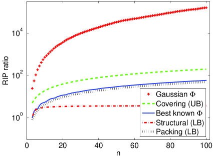
(a) $m=3$

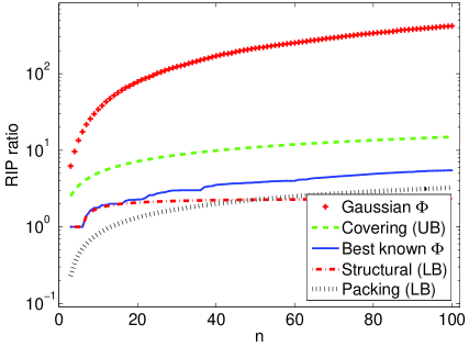
(b) $m=6$

(c) $m=8$

(d) $m=10$

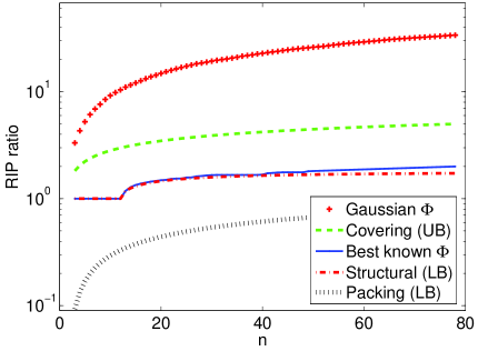
(e) $m=12$

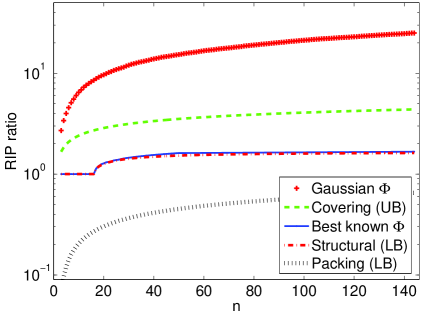
(f) $m=16$

Figure 1: RIP ratio bounds for $k=2$ and different values of $m$ and $n$. We compare the three bounds to the RIP ratio of Gaussian matrices as well as the best known matrix for the given problem size. The RIP ratio of Gaussian $\Phi$ shown is the geometric mean of the RIP ratio of 10,000 instantiations of randomly generated $m\times n$ Gaussian matrices. The RIP ratio of the best known $\Phi$ is based on the results of Conway, Hardin, and Sloane [35, 36, 37] on the best known packings in Grassmannian spaces.

The following observations can be made from Figure 1.

1. The Gaussian CS matrix construction has a much higher RIP ratio in comparison to the three bounds, revealing the existence of CS matrices in ${\mathbb{R}}^{m\times n}$ that will offer much better performance. Specifically, there is a substantial gap between the Gaussian RIP ratio and the achievable bound.

2. The best known CS matrix (obtained from the work of Conway, Hardin and Sloane [35, 36, 37]) in ${\mathbb{R}}^{m\times n}$ has an RIP ratio that is lower than the covering bound and greater than the structural and packing bounds. Therefore, we can think of the covering bound as an upper bound and the structural and packing bounds as lower bounds; together, they define a band within which the RIP ratio of the optimal CS matrix resides. Note that the best known $\Phi$ lies within this band. In fact, the RIP ratio curve for the best $\Phi$ performs significantly better than the achievable bound.

3. Regarding the converse bound, the structural bound is stronger for smaller values of $n$, whereas the packing bound is stronger for larger values of $n$. In fact, for $n<m(m+1)/2$, the best CS matrices are governed by the structural bound, whereas for $n>m(m+1)/2$, the packing bound governs the behavior. In Section III, we see the significance of this transition point in $n$ and relate it to equi-angular tight frames.

III Structural Bound for the RIP Ratio

In this Section, we prove Theorem 4 by first presenting a series of results. We also uncover the properties of the proposed lower bound on the RIP ratio.

III-A Bound for RIP Ratio when Singular Values of $\Phi$ are Known

First, we present a lower bound on the RIP ratio when the singular values of $\Phi$ are known.

Theorem 7

Let $\Phi$ be an ${m\times n}$ matrix over ${\mathbb{R}}$ or ${\mathbb{C}}$ and $0<m<n$. Let $S_{1}\geq S_{2}\geq...\geq S_{m}$ be the $m$ singular values of $\Phi$. Let the singular values of the submatrix $\Phi_{p}$ be $s_{p,1}\geq s_{p,2}\geq...\geq s_{p,k}$, for all $p\in\{1,2,...,{n\choose k}\}$. Let

$$g_{k}(x)=D^{n-k}\left[x^{n-m}(x-S_{1}^{2})(x-S_{2}^{2})...(x-S_{m}^{2})\right].$$ (19)

Let $r_{1}^{2}\geq r_{2}^{2}\geq...r_{k}^{2}$ be the zeros of $g_{k}(x)$. Then, the following results are true:

1. The $k$ zeros of $g_{k}(x)$ are real and lie in the interval $(0,S_{1}^{2}]$.

2. $\rho_{\max}(\Phi,k)\geq r_{1}^{2},~{}~{}\rho_{\min}(\Phi,k)\leq r_{k}^{2},~{}~{}\mbox{ and }~{}~{}R(\Phi,k)\geq\frac{r_{1}^{2}}{r_{k}^{2}}.$

3. Equality in all three inequalities above is attained if and only if the following two conditions are satisfied:

   1. The largest singular values of every $m\times k$ submatrix of $\Phi$ are all equal. That is, $s_{p,1}=s_{q,1}$ for all $p,q\in\{1,2,...,{n\choose k}\}$.

   2. The smallest singular values of every $m\times k$ submatrix of $\Phi$ are all equal. That is, $s_{p,k}=s_{q,k}$ for all $p,q\in\{1,2,...,{n\choose k}\}$.

The proof of this result hinges on a Theorem of Robert C. Thompson [27] that relates the singular values of all submatrices of a given size to the singular values of the complete matrix. We present the statement of Thompson’s Theorem here for completeness; its proof and other results on singular values and eigen values of submatrices are dealt with in  [40, 41, 42, 43, 44, 45, 46, 47, 27].

Theorem 8

[27, Theorem 4] Let $A$ be an $m\times n$ matrix with singular values $\alpha_{1}\geq\alpha_{2}\geq...\geq\alpha_{\min\{m,n\}}$. Let $B_{p}$ be an $l\times k$ submatrix of $A$ for some fixed $l\in\{1,2,...,m\}$ and $k\in\{1,2,...,n\}$ with singular values $\beta_{p,1}\geq\beta_{p,2}\geq...\geq\beta_{p,{\min\{l,k\}}}$, and index $p$ that identifies the submatrix amongst all $l\times k$ submatrices of $A$. Set

$$f_{p}(x) = (x-\beta_{p,1}^{2})(x-\beta_{p,2}^{2})...(x-\beta_{p,{\min\{l,k\}}}^{2}),$$

$$f(x) = (x-\alpha_{1}^{2})(x-\alpha_{2}^{2})...(x-\alpha_{{\min\{m,n\}}}^{2}).$$

Then, the following result is true:

$$\sum_{p}x^{l-\min\{l,k\}}f_{p}(x)=\frac{1}{(m-l)!}\frac{1}{(n-k)!}D^{m-l}\left[x^{m-k}D^{n-k}\left[x^{n-\min\{m,m\}}f(x)\right]\right],$$

where the summation is taken over all the submatrices of $A$ of size $l\times k$.

Proof of Theorem 7: The zeros of $g_{k}(x)$ are real and lie in the closed interval $[0,S_{1}^{2}]$ as a consequence of the Gauss-Lucas Theorem [48]. Recall that the Gauss-Lucas Theorem asserts that every convex set in the complex plane containing all the zeros of a polynomial also contains all its critical points (the zeros of the derivative of the chosen polynomial). In our setting, we consider the polynomial $G(x)=x^{n-m}(x-S_{1}^{2})(x-S_{2}^{2})...(x-S_{m}^{2})$ that has all its zeros in the closed interval $[0,S_{1}^{2}]$ on the real number line. Differentiating the polynomial $G(x)$ $(n-k)$ times and applying the Gauss-Lucas Theorem at each step, we infer that the $k$ zeros of $g_{k}(x)$ are real and lie in the interval $[0,S_{1}^{2}]$. Finally, we observe that $x=0$ cannot be a zero of the polynomial $g_{k}(x)$, because $x=0$ is a zero of $G(x)$ of order $(n-m)$, whereas we differentiate $(n-k)>(n-m)$ times. Thus we have established the first statement of Theorem 7.

To prove the second statement of Theorem 7, we apply Theorem 8 (Thompson’s Theorem) to our setting. Consider the complete matrix $\Phi$ of size ${m\times n}$ and the collection of ${m\times k}$ sized submatrices $\Phi_{p}$ for $p=1,2,...,{n\choose k}$. We obtain

$$\frac{1}{(n-k)!}D^{n-k}\left[x^{n-m}(x-S_{1}^{2})(x-S_{2}^{2})...(x-S_{m}^{2})\right]=\sum_{p}(x-s_{p,1}^{2})(x-s_{p,2}^{2})...(x-s_{p,k}^{2}).$$ (20)

The above equation relates the singular value polynomial of $\Phi$ to the singular value polynomials of the submatrices $\Phi_{p}$. Recall that the singular value polynomial of a matrix $A$ is the polynomial whose roots are the squares of the singular values of the matrix. Equation (20) asserts that the sum of the singular value polynomials of the submatrices $\Phi_{p}$ is a constant multiple of the $(n-k)$’th derivative of the singular value polynomial of $\Phi$.

Since $r_{1}^{2},r_{2}^{2},...,r_{k}^{2}$ are the roots of $g_{k}(x)$, we have

$$\frac{n!}{k!}(x-r_{1}^{2})(x-r_{2}^{2})...(x-r_{k}^{2})=D^{n-k}\left[x^{n-m}(x-S_{1}^{2})(x-S_{2}^{2})...(x-S_{m}^{2})\right],$$ (21)

where the constant $n!/k!$ is needed to equalize the coefficients of $x^{k}$ in the LHS and RHS. From (20) and (21), we have

$${n\choose k}(x-r_{1}^{2})(x-r_{2}^{2})...(x-r_{k}^{2})=\sum_{p}(x-s_{p,1}^{2})(x-s_{p,2}^{2})...(x-s_{p,k}^{2}).$$ (22)

We are now in a position to prove the second statement of Theorem 7. First, we note that $\rho_{\max}(\Phi,k)=\max_{p}\{s_{p,1}^{2}\}$ and $\rho_{\min}(\Phi,k)=\min_{p}\{s_{p,1}^{2}\}$. The first inequality in the second statement implies that $\max_{p}\{s_{p,1}^{2}\}\geq r_{1}^{2}$. For the sake of a contradiction, assume that $s_{p,1}^{2}<r_{1}^{2}$ for all $p\in\left\{1,2,...{n\choose k}\right\}$. Under this assumption, $(r_{1}^{2}-s_{p,i}^{2})>0$ for all $p$ and $i$ and hence each of the polynomial $(x-s_{p,1}^{2})(x-s_{p,2}^{2})...(x-s_{p,k}^{2})$ is strictly positive when evaluated at $x=r_{1}^{2}$. Consequently, the sum in the RHS of (22) evaluated at $x=r_{1}^{2}$ is strictly positive, which is a contradiction, because the LHS of (22) evaluates to zero for $x=r_{1}^{2}$. Therefore, we require $r_{1}^{2}\leq\max\{s_{p,1}^{2}\}=\rho_{\max}(\Phi,k)$.

We can show that $r_{k}^{2}\geq\max\{s_{p,k}^{2}\}=\rho_{\min}(\Phi,k)$ using a similar argument as above. Note that we need to consider the additional nuance of the sign of $(x-s_{p,1}^{2})(x-s_{p,2}^{2})...(x-s_{p,k}^{2})$ when evaluating at $x=r_{k}^{2}$ with the assumption $s_{p,k}^{2}>r_{k}^{2}$. The sign of $(x-s_{p,1}^{2})(x-s_{p,2}^{2})...(x-s_{p,k}^{2})$ is either positive or negative depending on whether $k$ is even or odd, respectively. Finally, since $\rho_{\max}(\Phi,k)\geq r_{1}^{2}$ and $\rho_{\min}(\Phi,k)\leq r_{k}^{2}$, we have $R(\Phi,k)\geq\frac{r_{1}^{2}}{r_{k}^{2}}$, and hence the second statement of Theorem 7 is established.

We now prove the third statement of Theorem 7. When $s_{p,1}^{2}$ are equal for all $p\in\{1,2,...,{n\choose k}\}$, we observe that with $x=s_{p,1}^{2}$, the RHS of (22) evaluates to zero. Hence $s_{p,1}^{2}$ must equal $r_{i}^{2}$ for some $i\in\{1,2,...,k\}$. Since we have established in the second statement of Theorem 7 that we cannot have a zero of $(x-r_{1}^{2})(x-r_{2}^{2})...(x-r_{k}^{2})$ greater than $s_{p,1}^{2}$, it follows that $r_{1}^{2}=s_{p,1}^{2}$ for all $p$. Similarly, when $s_{p,k}^{2}$ are equal for all possible $p$, we have $r_{k}^{2}=s_{p,k}^{2}$.

Conversely, suppose $r_{1}^{2}=\max\{s_{p,1}^{2}\}$ is true. For the sake of a contradiction assume that the values of $s_{p,1}^{2}$, $p\in\{1,2,...,{n\choose k}\}$ are not all equal. In particular, pick $p_{1}$ such that $s_{p_{1},1}^{2}<\max\{s_{p,1}^{2}\}$. Then the polynomial corresponding to $p=p_{1}$ within the summation in RHS in (22) is strictly positive when evaluated at $r_{1}^{2}$. Consequently, $r_{1}^{2}$ cannot be a zero of (22), yielding a contradiction. A similar argument applies to the case when $r_{k}^{2}=\min\{s_{p,k}^{2}\}$. Thus we have established the third statement of Theorem 7, and therefore the proof of Theorem 7 is complete. ∎

While Theorem 7 applies to the case where the singular values of the CS matrix $\Phi$ are known, Theorem 4 applies to all matrices $\Phi$ of size $m\times n$. In our quest for deterministic bounds for the RIP ratio, Theorem 4 therefore is of central importance. To establish Theorem 4, we explore the following question: what choice of $S_{1}^{2},S_{2}^{2},...,S_{m}^{2}$ gives the most conservative bound for the RIP ratio when we invoke Theorem 7? We show below (Theorem 12) that the ratio $\frac{r_{1}^{2}}{r_{k}^{2}}$ is minimized when all the singular values of $\Phi$ are equal. Therefore this minimum ratio serves as a universal bound for RIP applicable to all CS matrices $\Phi$ of size $m\times n$ and leads to the proof of Theorem 4. Toward this goal, we investigate the nature of the dependence of $r_{i}^{2}$ on $S_{1}^{2},S_{2}^{2},...,S_{m}^{2}$ in Section III-B.

III-B The Zeros of $g_{k}(x)$ and the Singular Values of $\Phi$

In this Section, we treat each $r_{i}^{2}$, $i\in\{1,2,...,k\}$ as a function of $m$ variables $S_{1}^{2},S_{2}^{2},...,S_{m}^{2}$ with the goal to determine the optimal choice of $S_{j}$’s that minimize the ratio $\frac{r_{1}^{2}}{r_{k}^{2}}$. The exact functional form is given in (21). First, we present how an infinitesimal increment in one of the $S_{j}^{2}$’s affects the values of $r_{i}^{2}$’s.

Theorem 9

Let $G(x)=x^{n-m}(x-S_{1}^{2})(x-S_{2}^{2})...(x-S_{m}^{2})$ and let $r_{1}^{2}\geq r_{2}^{2}\geq...\geq r_{k}^{2}$ be the zeros of the polynomial $g_{k}(x)=D^{n-k}[G(x)]$. Then, we have

$$\frac{\partial(r_{i}^{2})}{\partial(S_{j}^{2})} = \left[\frac{D^{n-k}\left(\frac{G(x)}{x-S_{j}^{2}}\right)}{D^{n-k+1}G(x)}\right]~{}~{}\mbox{evaluated at}~{}~{}{x=r_{i}^{2}}$$ (23)

$$= \left[x\frac{D^{n-k}\left(\frac{G(x)}{x-S_{j}^{2}}\right)}{\sum_{l=1}^{m}S_{l}^{2}D^{n-k}\left(\frac{G(x)}{x-S_{l}^{2}}\right)}\right]~{}~{}\mbox{evaluated at}~{}~{}{x=r_{i}^{2}}.$$

Proof: Taking the partial derivative of (21) with respect to the variable $S_{1}^{2}$ while keeping $S_{2}^{2},S_{3}^{2},...,S_{m}^{2}$ fixed, we have

$$\frac{n!}{k!}\frac{\partial}{\partial(S_{1}^{2})}(x-r_{1}^{2})...(x-r_{k}^{2})=\frac{\partial}{\partial(S_{1}^{2})}D^{n-k}\left[x^{n-m}(x-S_{1}^{2})...(x-S_{m}^{2})\right].$$ (24)

Treating the quantity inside the $D^{n-k}[\cdot]$ as a product of $(x-S_{1}^{2})$ and $x^{n-m}(x-S_{2}^{2})(x-S_{3}^{2})...(x-S_{m}^{2})$ and using Leibnitz’s Theorem [49] for the $(n-k)$’th derivative of a product, we obtain

$$D^{n-k}\left[x^{n-m}(x-S_{1}^{2})(x-S_{2}^{2})...(x-S_{m}^{2})\right]=(x-S_{1}^{2})D^{n-k}\left[x^{n-m}(x-S_{2}^{2})(x-S_{3}^{2})...(x-S_{m}^{2})\right]$$

$$+(n-k)D^{n-k-1}\left[x^{n-m}(x-S_{2}^{2})(x-S_{3}^{2})...(x-S_{m}^{2})\right].$$ (25)

Taking partial derivative with respect to $S_{1}^{2}$ (and noting that the second term of RHS in (25) is independent of $S_{1}^{2}$), we can rewrite the RHS of (24) as

$$\frac{\partial}{\partial(S_{1}^{2})}D^{n-k}\left[x^{n-m}(x-S_{1}^{2})(x-S_{2}^{2})...(x-S_{m}^{2})\right]$$

$$= -D^{n-k}\left[x^{n-m}(x-S_{2}^{2})(x-S_{3}^{2})...(x-S_{m}^{2})\right]$$ (26)

$$= -D^{n-k}\left[\frac{G(x)}{(x-S_{1}^{2})}\right].$$

Expanding the LHS of (24),

$$\frac{n!}{k!}\frac{\partial}{\partial(S_{1}^{2})}(x-r_{1}^{2})...(x-r_{k}^{2}) = -\frac{n!}{k!}\sum_{i=1}^{k}\left\{\left[\prod_{1\leq l\leq k,l\neq i}(x-r_{l}^{2})\right]\frac{\partial r_{i}^{2}}{\partial(S_{1}^{2})}\right\}.$$ (27)

Evaluating (27) at $x=r_{1}^{2}$ and noting that only one term in the summation in the RHS of (27) is non-zero, we obtain

$$\frac{n!}{k!}\left.\frac{\partial}{\partial(S_{1}^{2})}(x-r_{1}^{2})...(x-r_{k}^{2})\right|_{x=r_{i}^{2}} = -\left.\frac{n!}{k!}\left[\prod_{1\leq l\leq k,l\neq i}(x-r_{l}^{2})\right]\frac{\partial r_{i}^{2}}{\partial(S_{1}^{2})}\right|_{x=r_{i}^{2}}$$ (28)

$$= -\left.\frac{n!}{k!}\frac{\left[\prod_{1\leq l\leq k}(x-r_{l}^{2})\right]}{x-r_{1}^{2}}\frac{\partial r_{i}^{2}}{\partial(S_{1}^{2})}\right|_{x=r_{i}^{2}}$$

$$= -\left.\frac{D^{n-k}\left[G(x)\right]}{x-r_{1}^{2}}\frac{\partial(r_{1}^{2})}{\partial(S_{1}^{2})}\right|_{x=r_{i}^{2}}.$$

From (24), (26), and (28), we infer that

$$\frac{\partial(r_{i}^{2})}{\partial(S_{j}^{2})} = \left[\frac{D^{n-k}\left(\frac{G(x)}{x-S_{j}^{2}}\right)}{\frac{D^{n-k}G(x)}{x-r_{1}^{2}}}\right]~{}~{}\mbox{evaluated at}~{}~{}{x=r_{i}^{2}}.$$ (29)

Finally, we use the well known result that if a function $f(x)$ has a zero at $x=a$ of multiplicity 1 (i.e., a simple zero), then $f(x)/(x-a)$ evaluated at $x=a$ is equal to $D\left[f(x)\right]$ evaluated at $x=a$. Applying this result, we have that $D^{n-k}G(x)/(x-r_{1}^{2})$ evaluated at $x=r_{1}^{2}$ is equal to $D^{n-k+1}G(x)$ evaluated at $x=r_{1}^{2}$, since $r_{1}^{2}$ is a zero of $D^{n-k}G(x)$. Using this in (29), we deduce that

$$\frac{\partial(r_{i}^{2})}{\partial(S_{j}^{2})} = \left[\frac{D^{n-k}\left(\frac{G(x)}{x-S_{j}^{2}}\right)}{D^{n-k+1}G(x)}\right]~{}~{}\mbox{evaluated at}~{}~{}{x=r_{i}^{2}},$$ (30)

which proves the first part of Theorem 9.

To prove the second part, denote $S(x)=(x-S_{1}^{2})(x-S_{2}^{2})...(x-S_{m}^{2})$, and consider the quantity $D^{n-k+1}[xG(x)]$. We have

$$D^{n-k+1}[xG(x)] = D^{n-k}\left[D\left\{x^{n-m+1}S(x)\right\}\right]$$ (31)

$$= D^{n-k}\left[(n-m+1)x^{n-m}S(x)+x^{n-m+1}D[S(x)]\right]$$

$$= (n-m+1)D^{n-k}\left[x^{n-m}S(x)\right]+D^{n-k}\left[xD[S(x)]\right].$$

Alternately, we can use Leibnitz Theorem to expand $D^{n-k+1}[xG(x)]$, yielding

$$D^{n-k+1}[xG(x)] = (n-k+1)D^{n-k}\left[G(x)\right]+xD^{n-k+1}\left[x^{n-m}S(x)\right].$$ (32)

From (31) and (32), we have

$$(n-m+1)D^{n-k}\left[x^{n-m}S(x)\right] + D^{n-k}\left[xD[S(x)]\right]$$

$$=~{}~{}~{}(n-k+1)D^{n-k}\left[G(x)\right] + xD^{n-k+1}\left[x^{n-m}S(x)\right]$$ (33)

and therefore

$$D^{n-k}\left[x^{n-m+1}D[S(x)]\right] = (m-k)D^{n-k}\left[G(x)\right]+xD^{n-k+1}\left[G(x)\right].$$ (34)

Therefore,

$$D^{n-k+1}\left[x^{n-m}S(x)\right] = \frac{1}{x}\left\{D^{n-k}\left[x^{n-m+1}D[S(x)]\right]-(m-k)D^{n-k}\left[G(x)\right]\right\}$$ (35)

$$= \frac{1}{x}\left\{D^{n-k}\left[x^{n-m+1}D[S(x)]-mG(x)\right]+kD^{n-k}\left[G(x)\right]\right\}.$$

Since $D[S(x)]=S(x)\left\{\frac{1}{x-S_{1}^{2}}+...+\frac{1}{x-S_{m}^{2}}\right\}$, we have

$$x^{n-m+1}D[S(x)] = x^{n-m}S(x)\left\{\frac{x}{x-S_{1}^{2}}+...+\frac{x}{x-S_{m}^{2}}\right\}.$$ (36)

Rewriting $mD^{n-k}G(x)$ as

$$mD^{n-k}G(x) = D^{n-k}\left[x^{n-m}S(x)\left\{\frac{x-S_{1}^{2}}{x-S_{1}^{2}}+...+\frac{x-S_{m}^{2}}{x-S_{m}^{2}}\right\}\right]$$ (37)

and, subtracting (37) from (36), we obtain

$$D^{n-k}\left[x^{n-m+1}D[S(x)]\right] - mD^{n-k}G(x)$$ (38)

$$= ~{}~{}D^{n-k}\left[x^{n-m}S(x)\left\{\frac{S_{1}^{2}}{x-S_{1}^{2}}+...+\frac{S_{m}^{2}}{x-S_{m}^{2}}\right\}\right].$$

Plugging the above result in (35) yields

$$D^{n-k+1}\left[x^{n-m}S(x)\right] = \frac{1}{x}kD^{n-k}\left[G(x)\right]$$ (39)

$$+ \frac{1}{x}\left\{\sum_{l=1}^{m}S_{l}^{2}D^{n-k}\left(\frac{G(x)}{x-S_{l}^{2}}\right)\right\}.$$

Substituting (39) in (30) and evaluating at $x=r_{1}^{2}$ (noting that $D^{n-k}\left[G(x)\right]$ is zero at $x=r_{1}^{2}$), we obtain the result in (23) which completes the proof of Theorem 9. ∎

Remark 1

From (23), we have

$$S_{1}\frac{\partial(r_{i}^{2})}{\partial(S_{1}^{2})}+S_{2}\frac{\partial(r_{i}^{2})}{\partial(S_{2}^{2})}+...+S_{m}\frac{\partial(r_{i}^{2})}{\partial(S_{m}^{2})}=r_{i}^{2},$$ (40)

which we recognize as Euler’s condition for homogeneity of $r_{i}^{2}$ on $\{S_{1}^{2},S_{2}^{2},...,S_{m}^{2}\}$ of degree $1$ [49].

Remark 1 implies that when we write $r_{i}^{2}$ as a function of $\{S_{1}^{2},S_{2}^{2},...,S_{m}^{2}\}$, we have

$$r_{i}^{2}(aS_{1}^{2},aS_{2}^{2},...,aS_{m}^{2})=ar_{i}^{2}(S_{1}^{2},S_{2}^{2},...,S_{m}^{2}),$$ (41)

for all $a\in{\mathbb{R}}^{+}$. This result is in agreement with (21), because the homogeneity result can be derived from (21) by making a change of variable from $x$ to $ax$.

Theorem 10

Under the assumptions of Theorem 9,

$$\frac{\partial(r_{i}^{2})}{\partial(S_{j}^{2})}\geq 0.$$

Theorem 10 is significant, because it indicates that increasing $S_{j}^{2}$ for any $j$ can only increase the corresponding $r_{i}^{2}$’s. This fact can be exploited if our objective is to maximize the singular values of the submatrices of $\Phi$. In Donoho’s paper  [2], the condition CS1 requires the smallest singular values of the submatrices of $\Phi$ to exceed a positive constant. The above Theorem indicates the relationship of CS1 condition to the singular values of the complete matrix $\Phi$. Also, in any practical system, we have a bound on the maximum $S_{j}^{2}$’s that can be used, reminiscent of coding with power constraints [50]. In such a scenario, Theorem 10 indicates that the best choice for the $S_{j}^{2}$’s is when they are all equal to the maximum allowable bound. In order to prove Theorem 10, we require a result on interlacing polynomials.

Definition 3

Two non-constant polynomials $p(x)$ and $q(x)$ with real coefficients have weakly interlacing zeros if:

• their degrees are equal or differ by one,

• their zeros are all real, and

• there exists an ordering such that

  $$\alpha_{1}\leq\beta_{1}\leq\alpha_{2}\leq\beta_{2}\leq...\leq\alpha_{\nu}\leq\beta_{\nu}\leq...,$$ (42)

  where $\alpha_{1},\alpha_{2},...$ are the zeros of one polynomial and $\beta_{1},\beta_{2},...$ are the zeros of the other.

If, in the ordering of (42), no equality sign occurs, then $p(x)$ and $q(x)$ have strictly interlacing zeros.

We use the following result of Hermite and Kakeya [48] to prove Theorem 10.

Theorem 11

(Hermite-Kakeya) Let $p(x)$ and $q(x)$ be non-constant polynomials in $x$ with real coefficients. Then, $p(x)$ and $q(x)$ have strictly interlacing zeros if and only if, for all $\mu$, $\lambda\in{\mathbb{R}}$ such that $\lambda^{2}+\mu^{2}>0$, the polynomial $g(x)=\lambda p(x)+\mu q(x)$ has simple, real zeros.

Proof of Theorem 10: We demonstrate in this proof that the numerator and denominator polynomials in the RHS of (23) have the same sign when evaluated at $x=r_{i}^{2}$. Consider the three polynomials $p_{1}(x)=D^{n-k+1}[G(x)]$, $p_{2}(x)=D^{n-k}\left\{G(x)/(x-S_{j}^{2})\right\}$ and $q(x)=D^{n-k}[G(x)]$. Note that $p_{1}(x)$ and $p_{2}(x)$ are of degree $(k-1)$, while $q(x)$ is of degree $k$. We assert that

1. $p_{1}(x)$ and $q(x)$ have strictly interlacing zeros, and

2. $p_{2}(x)$ and $q(x)$ have strictly interlacing zeros.

The first statement above is a straightforward consequence of the interlacing property of a polynomial with real zeros and its derivative [48]; we note that $p_{1}(x)=D[q(x)]$. The second statement follows from a direct application of Hermite-Kakeya’s Theorem to $p_{2}(x)$ and $q(x)$. Consequently, for a given zero of $q(x)$, say $r_{i}^{2}$, there are an equal number of zeros of $p_{1}(x)$ and $p_{2}(x)$ to the left of $r_{i}^{2}$ on the real number line. Similarly, there are an equal number of zeros of $p_{1}(x)$ and $p_{2}(x)$ to the right of $r_{i}^{2}$ on the real number line. Lastly, note that the leading coefficients of all three polynomials (i.e., the coefficient of $x^{k}$ for $q(x)$ and the coefficients of $x^{k-1}$ for $p_{1}(x)$ and $p_{2}(x)$) are positive. Therefore, $p_{1}(x)$ and $p_{2}(x)$ have the same sign when evaluated at $x=r_{i}^{2}$, and hence the RHS of (23) is positive, completing the proof. ∎

Finally, we present the main Theorem in this Section, which shows that the choice of $S_{j}$’s that minimize the ratio $r_{1}^{2}/r_{k}^{2}$ is when the $S_{j}^{2}$’s are all equal.

Theorem 12

Under the assumptions of Theorem 9, the ratio $r_{1}^{2}/r_{k}^{2}$ is minimized when $S_{1}^{2}=S_{2}^{2}=...=S_{m}^{2}$.

Proof: In order to minimize $r_{1}^{2}/r_{k}^{2}$, we consider its partial derivatives with respect to the $S_{j}^{2}$’s. At the optimal location, we require the partial derivatives to be zero, i.e.,

$$\frac{\partial}{\partial(S_{j}^{2})}\left\{\frac{r_{1}^{2}}{r_{k}^{2}}\right\}=0 \Rightarrow \frac{1}{r_{k}^{2}}\left\{r_{k}^{2}\frac{\partial(r_{1}^{2})}{\partial(S_{j}^{2})}-r_{1}^{2}\frac{\partial(r_{k}^{2})}{\partial(S_{j}^{2})}\right\}=0,$$ (43)

$$\Rightarrow \frac{r_{1}^{2}}{r_{k}^{2}}\left\{\frac{1}{r_{1}^{2}}\frac{\partial(r_{1}^{2})}{\partial(S_{j}^{2})}-\frac{1}{r_{k}^{2}}\frac{\partial(r_{k}^{2})}{\partial(S_{j}^{2})}\right\}=0,$$

$$\Rightarrow \frac{1}{r_{1}^{2}}\frac{\partial(r_{1}^{2})}{\partial(S_{j}^{2})}=\frac{1}{r_{k}^{2}}\frac{\partial(r_{k}^{2})}{\partial(S_{j}^{2})}$$

for all the $S_{j}$’s. We show that the above condition is satisfied with the choice $S_{1}^{2}=S_{2}^{2}=...=S_{m}^{2}$. Assume that the $S_{j}^{2}$’s are all equal and non-zero, and denote their common value by $S^{2}$. Because of symmetry, the quantities $\frac{\partial(r_{i}^{2})}{\partial(S_{j}^{2})}$ are independent of the choice of $j$, and we denote the said quantity by $\frac{\partial(r_{i}^{2})}{\partial(S^{2})}$. Consequently, the terms in the summation of LHS in the Euler homogeneity equation (40) are all equal, and hence

$$\frac{\partial(r_{i}^{2})}{\partial(S^{2})}=\frac{r_{i}^{2}}{mS^{2}}.$$

Therefore, $\frac{1}{r_{i}^{2}}\frac{\partial(r_{i}^{2})}{\partial(S^{2})}$ is independent of the index $i$ and hence the condition (43) is satisfied. It remains to show that the optimal point just derived is a minimum. A rigorous analysis to prove minimality involves the computation of the Hessian matrix [49] of $\frac{r_{1}^{2}}{r_{k}^{2}}$ with respect to the $S_{j}^{2}$’s. However, the analysis quickly turns intractable. Instead, we fix $S_{1}^{2}=1$ and note that the only choice of the $S_{j}^{2}$’s for $j=2,3,...,k$ that satisfy the condition (43) is when they are all equal to unity. Thus, we can check the maxima or minima criteria by comparing the value of $\frac{r_{1}^{2}}{r_{k}^{2}}$ at $S_{j}^{2}=1$ to another choice for the set $\{S_{j}^{2}\}$. We pick the set $S_{1}^{2}=1,S_{2}^{2}=0,S_{3}^{2}=0,...,S_{m}^{2}=0$ for the purpose of comparison, and we immediately see that $\frac{r_{1}^{2}}{r_{k}^{2}}=\infty$ for this choice, because $r_{k}^{2}=0$. Therefore, the optimal point we have determined is a minimum. ∎

We remark that the above proof reveals that the ratio $r_{i_{1}}^{2}/r_{i_{2}}^{2}$ of any two roots $r_{i_{1}}^{2}$ and $r_{i_{2}}^{2}$ is minimized for a given $i_{1}$ and $i_{2}$ such that $i_{1}<i_{2}$. Finally, we note that Theorem 7 together with Theorem 12 proves Theorem 4, which is the main result of this Section.

III-C Properties of the Structural Bound

In this Section, we study the relationships between the structural bound given by Theorem 4 and the parameters $n$, $m$, and $k$ of Compressed Sensing. Clearly, the properties of the structural bound are tied to the properties of the polynomial $f_{k}(x)$ as defined in Theorem 4. We begin by first expressing $f_{k}(x)$ in the standard polynomial form, by carrying out the $(n-k)$’th order differentiation in (16). We obtain

$$f_{k}(x)=\sum_{j=0}^{k}(-1)^{k-j}\frac{{m\choose k-j}(n+j-k)!}{j!}x^{j}$$ (44)

and

$$g_{k}(x)=\sum_{j=0}^{k}(-1)^{k-j}\left(\sum S_{1}^{2}S_{2}^{2}...S_{k-j}^{2}\right)\frac{(n+j-k)!}{j!}x^{j}.$$ (45)

We ask if the form of $f_{k}(x)$ is similar to one of classic polynomials in the literature [48]. The ratio of successive terms of the polynomial suggests that $f_{k}(x)$ is a Gauss Hypergeometric function of the second kind:

$$\frac{c_{j}}{c_{j+1}} = \frac{(-1)^{k-j-1}{m\choose{k-j-1}}\frac{(n+j-k+1)!}{(j+1)!}x^{j+1}}{(-1)^{k-j}{m\choose{k-j}}\frac{(n+j-k)!}{j!}x^{j+1}}$$

$$= \frac{(j-k)(j+n-k+1)}{(j+m-k+1)(j+1)}x.$$

Therefore,

$$f_{k}(x) = c\cdot_{2}F_{1}\left(-k,n-k+1;m-k+1;x\right),$$

for some constant $c$. There is very little known about the location of the zeros of hyper-geometric functions of the kind described above [51]. However, algorithms to compute the zeros have been recently studied [52].

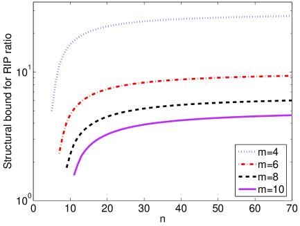
(a) $k=4$

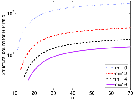
(b) $k=10$

Figure 2: Structural bound as a function of $n$. In each plot above, we fix $k$ to be a constant. Each curve is obtained for a given value of $m$.

To see the dependence of the structural bound on $n$, $m$ and $k$, we plot $r_{1}^{2}/r_{k}^{2}$ as a function of $n$ in Figure 2. We assume that the $S_{j}^{2}$’s are all equal. Several properties of the bound can be inferred from the plots. In particular,

1. For a given $m$ and $k$, the ratio $r_{1}^{2}/r_{k}^{2}$ increases when we increment $n$.

2. For a given $m$ and $k$, the ratio $r_{1}^{2}/r_{k}^{2}$ approaches a constant as we let $n\longrightarrow\infty$. In other words, $r_{1}^{2}/r_{k}^{2}$ can be upper bounded by a constant that is independent of $n$.

3. For a given $n$ and $m$, the ratio $r_{1}^{2}/r_{k}^{2}$ increases when we increment $k$.

4. For a given $n$ and $k$, the ratio $r_{1}^{2}/r_{k}^{2}$ decreases when we increment $m$.

Each of the statements above is stated and proved in the form of Theorems below. Alongside each Theorem, a result of the same flavor is proved for the RIP ratio for $\Phi$, if such a result exists.

The following Theorem shows that when we keep $m$ and $k$ fixed, the structural bound on the RIP ratio is an increasing function of $n$.

Theorem 13

Let $r_{1}^{2}>r_{2}^{2}>...>r_{k}^{2}$ be the zeros of the polynomial $D^{n-k}[x^{n-m}(x-1)^{m}]$, and let $t_{1}^{2}>t_{2}^{2}>...>t_{k}^{2}$ be the zeros of the polynomial $D^{(n+1)-k}[x^{(n+1)-m}(x-1)^{m}]$. Then,

$$\frac{r_{1}^{2}}{r_{k}^{2}}\leq\frac{t_{1}^{2}}{t_{k}^{2}}.$$

Proof: We have

$$D^{(n+1)-k}[x^{(n+1)-m}(x-1)^{m}] = D^{n-k}[D[x^{(n+1)-m}(x-1)^{m}]]$$ (46)

$$= D^{n-k}[(n+1-m)x^{n-m}(x-1)^{m}+mx^{(n+1)-m}(x-1)^{m-1}]$$

$$= D^{n-k}\left[x^{n-m}(x-1)^{m-1}\left\{(n+1-m)(x-1)+mx\right\}\right]$$

$$= (n+1)D^{n-k}\left[x^{n-m}(x-1)^{m-1}\left(x-\left(1-\frac{m}{n+1}\right)\right)\right].$$

Comparing (46) and (16) reveals that the polynomial $f_{k}(x)$ evaluated for $n+1$ and $m$ is of the same form (up to a constant) of $g_{k}(x)$ evaluated for $n$ and $k$ with all singular values equal except one with value $S_{m}^{2}=\left(1-\frac{m}{n+1}\right)$. Because the singular values are not all equal, Theorem 12 ensures that $\frac{r_{1}^{2}}{r_{k}^{2}}\leq\frac{t_{1}^{2}}{t_{k}^{2}}$. This completes the proof of Theorem 13. ∎

Theorem 14

Let $\Phi_{2}$ be an $m\times(n+1)$ sized matrix over ${\mathbb{R}}$ or ${\mathbb{C}}$, and let $\Phi_{1}$ be an $m\times n$ submatrix of $\Phi_{2}$. Then, the RIP ratios of the two matrices satisfy $R(\Phi_{1},k)\leq R(\Phi_{2},k)$.

Proof: Let $\Lambda_{1}$ be the set of all squared singular values $\{s_{p,i}^{2}\}$ of all submatrices of $\Phi_{1}$, and let $\Lambda_{2}$ be the set of all squared singular values of all submatrices of $\Phi_{2}$. Since every $m\times k$ submatrix of $\Phi_{1}$ is also a submatrix of $\Phi_{2}$, we have $\Lambda_{1}\subset\Lambda 2$. Therefore, $\max\{\Lambda_{1}\}\leq\max\{\Lambda_{2}\}$ and $\min\{\Lambda_{1}\}\geq\min\{\Lambda_{2}\}$. Because $R(\Phi_{1},k)=\max\{\Lambda_{1}\}/\min\{\Lambda_{1}\}$ and $R(\Phi_{2},k)=\max\{\Lambda_{2}\}/\min\{\Lambda_{2}\}$, the result of Theorem 14 follows as a consequence. ∎

The following Theorem shows that the structural bound can itself be bounded by a quantity that is independent of $n$.

Theorem 15

Let $r_{1}^{2}>r_{2}^{2}>...>r_{k}^{2}$ be the zeros of the polynomial $D^{n-k}[x^{n-m}(x-1)^{m}]$. Then,

$$\frac{r_{1}^{2}}{r_{k}^{2}}\leq\frac{(mk)^{k}(m-k)!}{m!}.$$ (47)

Proof: We establish the result by deriving an upper bound for $r_{1}^{2}$ and a lower bound for $r_{k}^{2}$. Applying Viéte’s Theorem to the polynomial in (44), we have

$$r_{1}^{2}+r_{2}^{2}+...+r_{k}^{2}=\frac{mk}{n}.$$

Since each term in the LHS of the above equation is positive, we have

$$r_{1}^{2}\leq\frac{mk}{n},$$ (48)

giving us an upper bound on $r_{1}^{2}$.

To derive a lower bound on $r_{k}^{2}$, we begin by using Viéte’s Theorem for the constant term of (44), involving the product $r_{1}^{2}r_{2}^{2}...r_{k}^{2}$:

$$r_{1}^{2}r_{2}^{2}...r_{k}^{2}=\frac{{m\choose k}}{{n\choose k}}.$$

Since $r_{i}^{2}>r_{k}^{2}$ for all $i<k$, we have the inequality

$$r_{k}^{2}(r_{1}^{2})^{k-1}\geq\frac{{m\choose k}}{{n\choose k}}.$$

Applying (48) to the above inequality, we have

$$r_{k}^{2}\left(\frac{mk}{n}\right)^{k-1}\geq r_{k}^{2}(r_{1}^{2})^{k-1}\geq\frac{{m\choose k}}{{n\choose k}}.$$

Therefore, we have

$$r_{k}^{2} \geq \frac{{m\choose k}}{{n\choose k}}\frac{n^{k-1}}{(mk)^{k-1}}$$ (49)

$$= \frac{m!(n-k)!n^{k-1}}{(m-k)!n!(mk)^{k-1}}$$

$$= \frac{m!}{n(m-k)!(mk)^{k-1}}\frac{(n-k)!n^{k}}{n!}$$

$$\geq \frac{m!}{n(m-k)!(mk)^{k-1}},$$

where the last inequality (49) is a consequence of $n^{k}\geq n!/(n-k)!$. Combining the inequalities (48) and (49) by taking the ratio (noting that both inequalities have positive LHS and RHS), we obtain the inequality in (47), completing the proof of Theorem 47. ∎

Although Theorem 47 gives an upper bound for the structural bound $r_{1}^{2}/r_{k}^{2}$ that is independent of $n$, we cannot bound the RIP ratio $R(\Phi,k)$ as we increase $n$. This is because $R(\Phi,k)$ necessarily increases with $n$. Consequently, as we increase $n$, the structural bound becomes more loose (this can be seen in Figure 1). The packing bound, discussed below in Section IV, provides a tighter bound for large $n$ because it captures the growth of $R(\Phi,k)$ with increasing $n$.

Theorem 16

Let $r_{1}^{2}>r_{2}^{2}>...>r_{k}^{2}$ be the zeros of the polynomial $D^{n-k}[x^{n-m}(x-1)^{m}]$, and let $t_{1}^{2}>t_{2}^{2}>...>t_{k}^{2}$ be the zeros of the polynomial $D^{n-k}[x^{n-m+1}(x-1)^{m-1}]$. Then,

$$\frac{r_{1}^{2}}{r_{k}^{2}}\leq\frac{t_{1}^{2}}{t_{k}^{2}}.$$

Proof: Reducing $m$ by one is equivalent to the following operation: set $S_{m}^{2}=0$. The proof of the above Theorem follows therefore from a straightforward application of Theorem 12. ∎

Theorem 17

Let $\Phi_{2}$ be an $(m+1)\times n$ sized matrix over ${\mathbb{R}}$ or ${\mathbb{C}}$, and let $\Phi_{1}$ be an $m\times n$ submatrix of $\Phi_{2}$. Then, the RIP ratios of the two matrices satisfy $R(\Phi_{1},k)\leq R(\Phi_{2},k)$.

Proof: Let $p\in\{1,2,...,{n\choose k}\}$ be the index that identifies the set of $k$ columns that are selected from the complete matrix to form a submatrix with $k$ columns. Then, $(\Phi_{1})_{p}$ is a submatrix of $(\Phi_{2})_{p}$, and consequently, the maximum (minimum) singular value of $(\Phi_{1})_{p}$ is smaller (greater) than the maximum (minimum) singular value of $(\Phi_{2})_{p}$ by the interlacing Theorem for matrices [27]. Thus Theorem 17 is established. ∎

Theorem 18

Let $r_{1}^{2}>r_{2}^{2}>...>r_{k}^{2}$ be the zeros of the polynomial $D^{n-k}[x^{n-m}(x-1)^{m}]$, and let $t_{1}^{2}>t_{2}^{2}>...>t_{k+1}^{2}$ be the zeros of the polynomial $D^{n-k-1}[x^{n-m+1}(x-1)^{m-1}]$. Then,

$$\frac{r_{1}^{2}}{r_{k}^{2}}\leq\frac{t_{1}^{2}}{t_{k+1}^{2}}.$$

Proof: Since $D^{n-k-1}[x^{n-m+1}(x-1)^{m-1}]=D\left[D^{n-k}[x^{n-m}(x-1)^{m}]\right]$, the roots of the two polynomials weakly interlace, as a consequence of the interlacing theorem for a polynomial and its derivative [48]. Therefore, $r_{1}^{2}\leq t_{1}^{2}$ and $r_{k}^{2}\geq t_{k+1}^{2}$ and the proof of Theorem 18 follows as a consequence. ∎

Finally, we state a similar Theorem for matrices.

Theorem 19

Let $\Phi$ be an $m\times n$ matrix over ${\mathbb{R}}$ or ${\mathbb{C}}$. Then, the RIP ratios satisfy $R(\Phi,k)\leq R(\Phi,k+1)$.

The proof of Theorem 19 is identical to the proof of Theorem 17.

III-D Geometric Interpretation

Recall the geometric interpretation of the SVD: The matrix $\Phi$ with SVD $\Phi=USV^{T}$ can be represented as a hyperellipse of dimension $m$ embedded in ${\mathbb{R}}^{n}$. The axes of the hyperellipse are aligned with the column vectors of $V$ with the length of each semi-axis equal to the corresponding singular value. Denote this hyperellipse by $E(\Phi)$. It is well known [53] that $\|\Phi x\|_{2}$ is equal to the magnitude of the projection of the vector $x$ onto the hyperellipse $E(\Phi)$. Furthermore, the column vectors of $U$ describe the orientation of the hyperellipse in ${\mathbb{R}}^{m}$, which is the image of $\Phi x$ of the unit sphere in ${\mathbb{R}}^{n}$. That is, for $\|x\|_{2}=1$ we have

$${n-q\choose k-q}\sum_{q-\mbox{wise}}(S_{1}S_{2}...S_{q})^{2}=\sum_{p}\left\{\sum_{q-\mbox{wise}}(s_{p,1}s_{p,2}...s_{p,q})^{2}\right\},$$ (50)

where the $q$-wise summation in (50) is the sum of all the terms that are obtained by multiplying $q$ unique singular values. Equation (50) relates the dimensions of $E(\Phi)$ to the dimensions of the collection of $k$-dimensional hyperellipses $E(\Phi_{p})$ corresponding to each $\Phi_{p}$. Note that each of the hyperellipses $E(\Phi_{p})$ lie in a $k$-dimensional subspace spanned by $k$ canonical basis vectors. A particularly interesting case is when $m=k=q$, for which (50) reduces to

$$(S_{1}S_{2}...S_{k})^{2}=\sum_{p}(s_{p,1}s_{p,2}...s_{p,k})^{2}.$$ (51)

The above result for $m=k=q$ is equivalent to the Generalized Pythagorean Theorem (GPT) [30, 31]. The GPT states that the square of the $k$-volume of a $k$-dimensional parallelepiped embedded in an $n$-dimensional Euclidean space is equal to the sum of the squares of the $k$-volumes of the ${n\choose k}$ projections of the parallelepiped on to the distinct $k$-dimensional subspaces spanned by the canonical basis vectors. Equation (51) implies that the statement of the GPT can be directly carried over from parallelepipeds to hyperellipses.

Equation (50) extends GPT to arbitrary values of $m$, $k$ and $q$. The form of the equation motivates us to define the $q$-volume of an ellipse of intrinsic dimension that is greater than $q$ as follows.

Definition 4

Consider a hyperellipse $H$ of dimension $d>q$ with semi-axes $a_{1},a_{2},...,a_{d}$. The $q$-volume of $H$, denoted by $\mbox{Vol}_{q}(H)$, is defined as

$$\mbox{Vol}_{q}(H)\triangleq\sqrt{\sum_{q-\mbox{wise}}(a_{1}a_{2}...a_{q})^{2}}.$$

Equation (50) therefore relates the $q$-volumes of $E(\Phi)$ to the $q$-volumes of $E(\Phi_{p})$ in the following manner: the square of the $q$-volume of $E(\Phi)$ is proportional to the sum of the squares of the $q$-volumes of $E(\Phi_{p})$.

III-E Structural Bound for $k=2$

In this subsection, we study the structural bound for the specific case of $k=2$. The motivation for studying this case are many fold. First, $k=2$ is the smallest non-trivial case to investigate the RIP ratio. For the case $k=1$, any matrix $\Phi$ that has equi-normed columns satisfies $R(\Phi,1)=1$, and therefore the structural bound is trivially $1$ for any $n$ and $m$. Secondly, the roots of the polynomial (44) can be explicitly evaluated, providing an avenue for analysis. Lastly and most importantly, designing good CS matrices for $k=2$ can be shown to be equivalent to well-known problems in coding theory.

For $k=2$, the form of (44) and (45) reduce to

$$\frac{n(n-1)}{2}x^{2}-\left(\sum_{j=1}^{m}S_{j}^{2}\right)(n-1)x+\left(\sum_{1\leq j_{1}<j_{2}\leq m}S_{j_{1}}^{2}S_{j_{2}}^{2}\right)=0$$ (52)

and

$$\frac{n(n-1)}{2}x^{2}-(n-1)mx+\frac{m(m-1)}{2}=0.$$ (53)

We focus on (53), because we are interested in universal bounds for the RIP ratio. The roots of (53) can be computed as

$$r_{1}^{2},r_{2}^{2}=\frac{m}{n}\pm\frac{1}{n}\sqrt{\frac{m(n-m)}{n-1}},$$

and the structural bound is thus

$$\frac{r_{1}^{2}}{r_{2}^{2}}=\frac{1+\sqrt{\frac{n-m}{m(n-1)}}}{1-\sqrt{\frac{n-m}{m(n-1)}}}.$$

Note that as $n\longrightarrow\infty$, the above equation reduces to

$$\lim_{n\longrightarrow\infty}\frac{r_{1}^{2}}{r_{2}^{2}}\mbox{~{}~{}}=\mbox{~{}~{}}\frac{1+\sqrt{\frac{1}{m}}}{1-\sqrt{\frac{1}{m}}}\mbox{~{}~{}}=\mbox{~{}~{}}\frac{\left(1+\sqrt{\frac{1}{m}}\right)^{2}}{1-\frac{1}{m}}.$$ (54)

Recall that we derived an upper bound (47) on $\frac{r_{1}^{2}}{r_{2}^{2}}$ that is applicable for any $m$, $k$ and as $n\longrightarrow\infty$. Substituting $k=2$ in (47), we obtain

$$\frac{r_{1}^{2}}{r_{k}^{2}}\mbox{~{}~{}}\leq\mbox{~{}~{}}\frac{(2m)^{2}(m-2)!}{m!}\mbox{~{}~{}}=\mbox{~{}~{}}\frac{4m^{2}}{m(m-1)}\mbox{~{}~{}}=\mbox{~{}~{}}\frac{4}{1-\frac{1}{m}}.$$ (55)

Comparison of (54) and (55) reveals that (54) offers a tighter bound on $r_{1}^{2}/r_{k}^{2}$ than (55).

We now make some interesting connections between good CS matrices for $k=2$ and coding theory. The key result that provides the segue is Theorem 20.

Theorem 20

Let $A=\left[a_{1}~{}~{}a_{2}~{}~{}a_{3}~{}...~{}a_{n}\right]$ be an $m\times n$ matrix over ${\mathbb{R}}$ or ${\mathbb{C}}$ comprising $n\geq 2$ columns $a_{1},a_{2},...a_{n}$ of size $m\times 1$, with $\|a_{i}\|_{2}>0$. Construct the $m\times n$ matrix $B$ as

$$B=\left[\frac{a_{1}}{\|a_{1}\|_{2}}~{}~{}\frac{a_{2}}{\|a_{2}\|_{2}}~{}~{}\frac{a_{3}}{\|a_{3}\|_{2}}~{}...~{}~{}~{}\frac{a_{n}}{\|a_{n}\|_{2}}\right],$$ (56)

obtained by scaling every column of $A$ independently so that the $\ell_{2}$ norm of every column of $B$ is unity. Then, the RIP ratios of $A$ and $B$ satisfy $R(B,2)\leq R(A,2)$.

Proof: We prove the Theorem by considering two cases: $n=2$ and $n>2$.
Case 1: $n=2$.
Since $A$ has only two columns, the only submatrix of $A$ of size $m\times 2$ is $A$ itself. Therefore, the RIP ratio is simply the ratio of the square of the two singular values of $A$. Let the $\ell_{2}$ norms of column vectors $a_{1}$ and $a_{2}$ be $\|a_{1}\|_{2}=d_{1}$ and $\|a_{2}\|_{2}=d_{2}$. Let the angular distance between $a_{1}$ and $a_{2}$ be $\theta$, given by $\cos(\theta)=|\left<a_{1}\cdot a_{2}\right>|/(d_{1}d_{2})$, where $|\left<a_{1}\cdot a_{2}\right>|$ is the absolute value of the dot product of $a_{1}$ and $a_{2}$.

Let $S_{1}^{2}$ and $S_{2}^{2}$ be the squared singular values of $A$, with $S_{1}^{2}\geq S_{2}^{2}$. Since the squared singular values of $A$ are the eigen values of the grammian matrix $A^{H}A$, we compute $A^{H}A$ as

$$A^{H}A=\left(\begin{array}[]{cc}d_{1}^{2}&d_{1}d_{2}\cos(\theta)\\ d_{1}d_{2}\cos(\theta)&d_{2}^{2}\end{array}\right).$$ (57)

Thus $S_{1}^{2}$ and $S_{2}^{2}$ are the zeros of the characteristic polynomial of (57) given by $x^{2}-(d_{1}^{2}+d_{2}^{2})^{2}+\left(d_{1}d_{2}\right)^{2}\sin^{2}(\theta)$. Computing the roots of this polynomial yields

$$S_{1}^{2}=\frac{1}{2}\left[d_{1}^{2}+d_{2}^{2}+\sqrt{\left(d_{1}^{2}+d_{2}^{2}\right)^{2}-4\left(d_{1}d_{2}\right)^{2}\sin^{2}(\theta)}\right]$$

and

$$S_{2}^{2}=\frac{1}{2}\left[d_{1}^{2}+d_{2}^{2}-\sqrt{\left(d_{1}^{2}+d_{2}^{2}\right)^{2}-4\left(d_{1}d_{2}\right)^{2}\sin^{2}(\theta)}\right].$$

The RIP ratio of $A$ is given by

$$R(A,2)=\frac{S_{1}^{2}}{S_{2}^{2}} = \frac{d_{1}^{2}+d_{2}^{2}+\sqrt{\left(d_{1}^{2}+d_{2}^{2}\right)^{2}-4\left(d_{1}d_{2}\right)^{2}\sin^{2}(\theta)}}{d_{1}^{2}+d_{2}^{2}-\sqrt{\left(d_{1}^{2}+d_{2}^{2}\right)^{2}-4\left(d_{1}d_{2}\right)^{2}\sin^{2}(\theta)}}$$ (58)

$$= \frac{1+\sqrt{1-\nu\sin^{2}(\theta)}}{1-\sqrt{1-\nu\sin^{2}(\theta)}},$$

where

$$\nu=\frac{\left(2d_{1}d_{2}\right)}{d_{1}^{2}+d_{2}^{2}}$$

is the ratio of the geometric mean and the arithmetic mean of $d_{1}^{2}$ and $d_{2}^{2}$. From (58), we infer that in order to minimize $R(A,2)$ for a fixed $\theta$, we require $\nu$ to be as large as possible. Since $\nu$ is the ratio of geometric mean and arithmetic mean of $d_{1}^{2}$ and $d_{2}^{2}$, maximum value of $\nu$ is attained when $d_{1}=d_{2}$, yielding $\nu_{\max}=1$.

Since the angular separation of the column vectors remains invariant while constructing $B$ from $A$ using (56), and we have equal column norms in $B$, we infer that $R(B,2)\leq R(A,2)$ from the above arguments. Thus we have proved Theorem 20 for the case $n=2$.

Note that when $d_{1}=d_{2}=d$, we have

$$S_{1}^{2}=d^{2}\left(1+\cos(\theta)\right),$$ (59)

$$S_{2}^{2}=d^{2}\left(1-\cos(\theta)\right),$$ (60)

and

$$\frac{S_{1}^{2}}{S_{2}^{2}}=\frac{1+\cos(\theta)}{1-\cos(\theta)}=\cot^{2}\frac{\theta}{2}.$$ (61)

While Case 1 is applicable to matrices with two columns, we extend the result to include any $m\times n$ matrix in Case 2.
Case 2: $n>2$.
Consider the following three $m\times 2$ sized submatrices $A_{p_{0}}$, $A_{p_{1}}$, and $A_{p_{2}}$ of $A$, where $p_{0},p_{1},p_{2}$ are indices from $1,2,...,{n\choose 2}$:

1. $A_{p_{0}}$ is obtained by selecting the two columns of $A$ that have the minimum angular distance among all pairs of column vectors of $A$. Let the singular values of $A_{p_{0}}$ be $s_{p_{0},1}$ and $s_{p_{0},2}$ with $s_{p_{0},1}\geq s_{p_{0},2}$.

2. $A_{p_{1}}$ is the $m\times 2$ submatrix of $A$ whose largest singular value $s_{p_{1},1}$ is the maximum of all singular values of submatrices of $A$ of size $m\times 2$. In other words,

   $$p_{1}=\arg\max_{p}\{s_{p,1}\},\mbox{~{}~{}~{}~{}~{}~{}~{}~{}$p=1,2,...,{n\choose 2}$}.$$

   Let the singular values of $A_{p_{1}}$ be $s_{p_{1},1}$ and $s_{p_{1},2}$ with $s_{p_{1},1}\geq s_{p_{1},2}$.

3. $A_{p_{2}}$ is the $m\times 2$ submatrix of $A$ whose smallest singular value $s_{p_{2},2}$ is the minimum of all singular values of submatrices of $A$ of size $m\times 2$. In other words,

   $$p_{2}=\arg\min_{p}\{s_{p,2}\},\mbox{~{}~{}~{}~{}~{}~{}~{}~{}$p=1,2,...,{n\choose 2}$}.$$

   Let the singular values of $A_{p_{2}}$ be $s_{p_{2},1}$ and $s_{p_{2},2}$ with $s_{p_{2},1}\geq s_{p_{2},2}$.

We also consider an $m\times 2$ submatrix $B_{p_{0}}$ of $B$, using the same index $p_{0}$ defined above. The angular separation between column vectors are invariant to scaling of columns; therefore $B_{p_{0}}$ contains the two columns of $B$ that have the minimum angular distance among all pairs of column vectors of $B$. We denote the singular values of $B_{p_{0}}$ as $t_{1}$ and $t_{2}$ with $t_{1}\geq t_{2}$.
From the definition of RIP ratio, we have

$$R(A,2)=\frac{s_{p_{1},1}^{2}}{s_{p_{2},2}^{2}}.$$ (62)

Since $s_{p_{1},1}\geq s_{p_{0},1}$ and $s_{p_{2},2}\leq s_{p_{0},2}$, we have

$$\frac{s_{p_{1},1}^{2}}{s_{p_{2},2}^{2}}\geq\frac{s_{p_{0},1}^{2}}{s_{p_{0},2}^{2}}.$$ (63)

Invoking the result we have established from Case 1 for the $m\times 2$ sized matrices $A_{p_{0}}$ and $B_{p_{0}}$, we have $R(A_{p_{0}},2)\geq R(B_{p_{0}},2)$ and so

$$\frac{s_{p_{0},1}^{2}}{s_{p_{0},2}^{2}}\geq\frac{t_{1}^{2}}{t_{2}^{2}}.$$ (64)

Let us consider the RIP ratio of the matrix $B$. Since every column of $B$ has equal norm, we assert that the RIP ratio of $B$ is governed completely by the submatrix $B_{p_{0}}$. To see this, we first note that when the column norms are equal, the condition number of an $m\times 2$ matrix is dictated only by the angular separation of its two constituent column vectors. Specifically, if the two columns of an $m\times 2$ matrix have equal $\ell_{2}$ norm of $d$ and their angular separation is $\theta$, then the squared singular values are given by (59) and (60). Furthermore, the squared condition number is given by (61). The squared condition number is a monotonically decreasing function of $\theta$ in the range $0\leq\theta\leq\pi/2$. Therefore, the RIP ratio of $B$ is given by

$$R(B,2)=\frac{t_{1}^{2}}{t_{2}^{2}}.$$ (65)

Using the results of (62), (63), (64) and (65) and cascading the inequalities, we obtain $R(A,2)\geq R(B,2)$, and so the proof of Theorem 20 is complete. ∎

The above Theorem has important consequences for the RIP ratio of order $k=2$.

Remark 2

Theorem 20 reveals that among the set of all matrices that can be obtained by scaling each column of a given matrix independently, the RIP ratio for $k=2$ is minimized when the column norms are all equal.

We use the above results to study the properties of a CS matrix $\Phi$ that attains the structural bound for $k=2$. First, Theorem 4 (third statement) requires that $\Phi_{p}$ has the same pair of squared singular values for all $p$. Second, we deduce from Theorem 20 that the columns of $\Phi$ are all equi-normed. If the contrary were true, then equalizing the column norms will yield a matrix with smaller RIP ratio, which violates Theorem 4. Since this result is of importance, we state it in the form of a Theorem.

Theorem 21

If an $m\times n$ matrix $\Phi$ over ${\mathbb{R}}$ or ${\mathbb{C}}$ satisfies (17) with equality, then $\Phi$ has equi-normed columns.

Furthermore, we show that $\Phi$ that satisfies (17) with equality is an equi-angular tight frame (ETF) [28]. From [28, 29], we list the three conditions for a matrix $A$ to be an ETF:

1. The columns of $A$ are unit normed,

2. The absolute values of the dot product of every pair of columns of $A$ are same, i.e., the columns are equi-angular.

3. $AA^{*}=(n/m)I_{m\times m}$.

Theorem 22

Let an $m\times n$ matrix $\Phi$ over ${\mathbb{R}}$ or ${\mathbb{C}}$ satisfy (17) with equality, and let $\Phi$ be scaled such that its $m$ squared singular values are equal to $n/m$ each, i.e., $S_{1}^{2}=S_{2}^{2}=...S_{m}^{2}=n/m$. Then, $\Phi$ is an ETF.

Proof: Let $\Phi=USV^{*}$ be the singular value decomposition for $\Phi$. We check the three conditions for ETF, starting with the third condition. We have $AA^{*}=USV^{*}VSU^{*}=US^{2}U^{*}=(n/m)UIU^{*}=(n/m)I$, satisfying the third condition. The second condition is satisfied because every pair of columns have the same set of singular values. If the angle between two equi-normed columns is $\theta$ and the common norm is $d$, then the squared singular values of the $m\times 2$ sized submatrix comprising only of the two said columns are given by (59) and (60). To verify the first condition, we note that the norms of each column of $\Phi$ are the same, say $d^{2}$. It remains to show that this norm is unity. Substituting $S_{1}^{2}=S_{2}^{2}=...S_{m}^{2}=n/m$ in (52), we see that $s_{1}^{2}$ and $s_{2}^{2}$ are the roots of the quadratic equation

$$x^{2}-2x+\frac{n(m-1)}{m(n-1)}=0.$$ (66)

Therefore the sum of the roots of the quadratic equation is given by

$$s_{1}^{2}+s_{2}^{2}=2.$$ (67)

From (59) and (60), we have

$$s_{1}^{2}+s_{2}^{2}=2d^{2},$$ (68)

and hence we infer that $d^{2}=1$ by comparing (67) and (68). Thus $\Phi$ satisfies all three conditions for an ETF. ∎

The relationship between the structural bound and ETFs can be used to make statements about the set of allowable pairs $(m,n)$ that meet the structural bound. Results from [28] reveal that an ETF of size $m\times n$ exists only when $n\leq\frac{1}{2}m(m+1)$ for real ETFs and $n\leq m^{2}$ for complex ETFs. In addition, $n$ and $m$ should satisfy strict integer constraints.

III-F Structural Bound as Extension of the Welch Bound

Definition 5

The coherence of a matrix $A$, denoted by $\mu(A)$ is defined as the largest absolute inner product between any two columns $a_{i}$, $a_{j}$ of $A$. That is, for $A$ with $n$ columns,

$$\mu(A)=\max_{i,j\in\{1,2,...n\},i\neq j}\frac{|\left<a_{i}\cdot a_{j}\right>|}{\|a_{i}\|_{2}\|a_{j}\|_{2}}.$$ (69)

Recall the classical result of Welch that states that the coherence of a $m\times n$ matrix in ${\mathbb{R}}$ or ${\mathbb{C}}$ is always greater than or equal to $\sqrt{\frac{n-m}{m(n-1)}}$. It is well known that $\Phi$ is an ETF if and only if the coherence of $\Phi$ satisfies the Welch bound with equality [29, 28]. As a consequence of Theorem 22, we infer that if $\Phi$ satisfies (17) with equality, then the coherence of $\Phi$ meets the Welch bound.

We make the claim that the structural bound for $k>2$ extends the Welch bound from pairs of column vectors of a matrix to $k$-tuples of column vectors. We use the least singular value of a submatrix as a way to extend the notion of coherence to a $k$-tuple of vectors. Specifically, we wish to maximize the (normalized) least singular value of the submatrices in order to keep the submatrices as far apart as possible, in some sense. However, Theorem 7 asserts that the least singular value has an upper bound. Based on this insight, we extend the Welch bound explicitly in the following Theorem.

Theorem 23

(Extension of Welch Bound) Let $\Phi$ be an $m\times n$ matrix over ${\mathbb{R}}$ or ${\mathbb{C}}$ with $0<m<n$. Let $k$ be an integer such that $0<k<m$, and let $f_{k}(x)$ be the $k$’th degree polynomial given by $f_{k}(x)=D^{n-k}\left[x^{n-m}(x-1)^{m}\right]$. Let $r_{1}^{2}\geq r_{2}^{2}\geq...\geq r_{k}^{2}$ be the zeros of $f_{k}(x)$. Let $S_{1}$ be the largest singular value of $\Phi$. Let $s_{p,1}\geq s_{p,2}\geq...\geq s_{p,k},$ be the $k$ singular values of the $m\times k$ sized submatrix $\Phi_{p}$ of $\Phi$, where $p\in\{1,2,...,{n\choose k}\}$ is the index that identifies the submatrix. Then the smallest $s_{p,k}$, after normalization by $S_{1}^{2}$, is bounded by

$$\left(\frac{\min_{p}\{s_{p,k}^{2}\}}{S_{1}^{2}}\right)\leq r_{k}^{2}.$$ (70)

Proof: Let $S_{1}\geq S_{2}\geq...\geq S_{m}\geq 0$ be the $m$ singular values of $\Phi$. Define two more polynomials $g_{k}(x)$ and $h_{k}(x)$, both of degree $k$, given by

$$g_{k}(x)=D^{n-k}\left[x^{n-m}(x-S_{1}^{2})(x-S_{2}^{2})...(x-S_{m}^{2})\right]~{}~{}\mbox{ and }~{}~{}h_{k}(x)=D^{n-k}\left[x^{n-m}(x-S_{1}^{2})^{m}\right].$$

Let the zeros of $g_{k}(x)$ be $t_{1}^{2}\geq t_{2}^{2}\geq...\geq t_{k}^{2}$, and the zeros of $h_{k}(x)$ be $u_{1}^{2}\geq u_{2}^{2}\geq...\geq u_{k}^{2}$.
Based on the result of Theorem 7, we have

$$\min_{p}\{s_{p,k}^{2}\}\leq t_{k}^{2}.$$ (71)

From Theorem 10, we see that $t_{i}^{2}\leq u_{i}^{2}$ for all $i=1,2,...,k$, because we can think of the polynomial $h_{k}(x)$ as being obtained by increasing each of $S_{2}^{2},S_{3}^{2},...,S_{m}^{2}$ to $S_{1}^{2}$. Theorem 10 guarantees that the zeros of $h_{k}(x)$ are greater than the corresponding zeros of $g_{k}(x)$. Therefore, $t_{k}^{2}\leq u_{k}^{2}$ and so

$$\min_{p}\{s_{p,k}^{2}\}\leq u_{k}^{2}.$$ (72)

While (71) is a tighter bound than (72), the latter equation has the advantage that it depends only on $S_{1}^{2}$ and holds for all values of $S_{i}^{2}\leq S_{1}^{2}$, for $i=2,3,...,m$. In the final step of the proof, we use the result $u_{i}^{2}=S_{1}^{2}r_{i}^{2}$ which follows by noting that $h_{k}(x)$ is obtained by making the change of variable $x\rightarrow S_{1}x$ in $f_{k}(x)$. Substituting in (72), we obtain $\min_{p}\{s_{p,k}^{2}\}\leq S_{1}^{2}r_{k}^{2}$ and the proof is complete. ∎Based on the proof of Theorem 7, we infer that (70) holds with equality if and only if $s_{p,k}=S_{1}^{2}r_{k}^{2}$ for all $p\in\{1,2,...,{n\choose k}\}$. This extends the notion of ETFs, which for $k=2$, require only the angular separation between every pair of column vectors to be the same. Note that a necessary condition for the equality of (70) to hold is that $S_{1}^{2}=S_{2}^{2}=...=S_{m}^{2}$. Recently, Datta, Howard and Cochran have also proposed extensions to the Welch bound [54].

IV Packing and Covering Bounds for the RIP Ratio

The motivation to derive another bound for the RIP ratio comes from the perspective that we can view the CS matrix $\Phi$ as a collection of column vectors in ${\mathbb{R}}^{m}$. We need to spread these vectors as far away from each other as possible in order to ensure that the singular values of its $k$-column submatrices have good condition numbers. Increasing the number of columns (i.e., increasing $n$) leads to crowding of these vectors in ${\mathbb{R}}^{m}$ that leads to a deterioration of the RIP ratio. We make these notions precise for $k=2$. For $k>2$, the exact nature of the packing bounds are yet elusive.

As we saw from Theorem 20, we need restrict our attention only to matrices of equi-normed columns. Therefore, the problem of designing good CS matrices for $k=2$ is equivalent to finding arrangements of $n$ lines in ${\mathbb{R}}^{m}$ such that the minimum angle between the pairs of lines is maximized. This problem has been studied extensively by Conway, Hardin, and Sloane [35]. Furthermore, converse and achievable bounds can been derived by studying a related problem, namely of arrangements of $2n$ points on a Euclidean sphere in ${\mathbb{R}}^{m}$. The latter problem has been studied independently by Chabauty, Shannon, and Wyner [32, 33, 34]. We state the main results that are relevant to our problem of bounding the RIP ratio. For a detailed description and derivation of the relevant results from coding theory, see  [55].

Definition 6

The area of a spherical cap of radius $\beta$ on an $m$ dimensional Euclidean sphere of unit length is given by

$$C_{m}(\beta)=k_{m}\int_{0}^{\beta}\sin^{m-2}\alpha d\alpha,$$

where $k_{m}$ is given by

$$k_{m}=\frac{2\pi^{(m-1)/2}}{\Gamma\left(\frac{m-1}{2}\right)}.$$

Note that $2C_{m}(\pi)$ gives the surface area of a unit sphere in ${\mathbb{R}}^{m}$. Packing the surface of the $m$-dimensional sphere using spherical caps gives rise to an upper bound on the minimum angle $\theta$ that can be attained between the pairs of $2n$ points on the sphere. The upper bound $\theta_{\max}$ is given by $C_{m}\left(\frac{\theta_{\max}}{2}\right)=\frac{C_{m}(\pi)}{n}$. Consequently, we obtain a lower bound on the RIP ratio, which is captured in Theorem 5 as the packing bound.
Proof of Theorem 5: Using (61) to relate the minimum angular separation $\theta$ and the RIP ratio $R(\Phi,2)$, we obtain

$$R(\Phi,2)=\frac{1+\cos(\theta)}{1-\cos(\theta)}=\cot^{2}\left(\frac{\theta}{2}\right).$$ (73)

The statement follows from the fact that for any arrangement of $2n$ points on the surface of the unit sphere in ${\mathbb{R}}^{m}$, the minimum angle between pairs of points is less than $\theta$ defined above, as a result of packing. Note that the form of Theorem 5 is obtained by making a change of variable $\theta/2\rightarrow\theta$. ∎

Furthermore, covering arguments can be used to make a statement on achievability. Based on the results of Chabauty, Shannon, and Wyner [32, 33, 34, 55, 56] we can guarantee the existence of an arrangement of $2n$ points on the Euclidean sphere in ${\mathbb{R}}^{m}$ where the angular distance between every pair of points is at least as large as $\theta$, where $C_{m}(\theta)=\frac{C_{m}(\pi)}{n}$. Theorem 6 captures the achievable bound on the RIP ratio obtained using the above arguments.

While we have successfully derived the structural bound for any $n$, $m$ and $k$, the derivation of packing and covering bounds for $k>2$ remains an open problem. The main challenge is that Theorem 20 cannot be extended beyond $k=2$. In fact, it is easy to construct matrices where the RIP ratio for $k>2$ increases when we equalize the column norms.

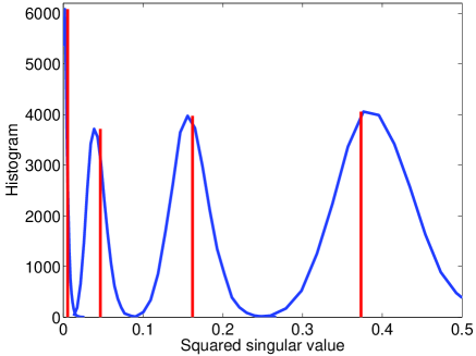
(a) $n=100$, $m=14$, $k=12$

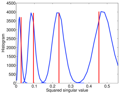
(b) $n=100$, $m=20$, $k=12$

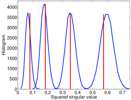
(c) $n=100$, $m=30$, $k=12$

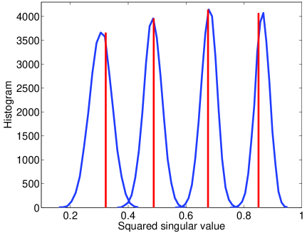
(d) $n=100$, $m=60$, $k=12$

Figure 3: Histograms of the squared singular values of submatrices of $\Phi$. In each of the plots, we fix $n$, $m$ and $k$. We then plot, in the same figure, the histograms for the $1$st, $4$th, $8$th and $12$th squared singular values $s_{p,1}^{2}$, $s_{p,4}^{2}$, $s_{p,8}^{2}$, and $s_{p,12}^{2}$ of $25,000$ randomly chosen $m\times k$ sized submatrices of $\Phi$. The complete matrix $\Phi$ is chosen with $m$ prescribed singular values all equal to unity. The four red vertical lines in each plot correspond to the values of the $1$st, $4$th, $8$th and $12$th zeros of the polynomial in (19). Note the excellent match between the histogram peaks and the polynomial zeros; this observation suggests that the zeros of the polynomial in (19) are in fact estimators (a mean, in some sense) of the squared singular values of randomly chosen $m\times k$ submatrices of $\Phi$.

V Relevance of the Structural Bounds in Statistical RIP

It can be argued that the definition of RIP is too restrictive in the sense that the RIP constant $\delta_{k}$ and the RIP ratio $R(\Phi,k)$ depend on extremal values of the singular values of the submatrices. Because the number ${n\choose k}$ of submatrices of $\Phi$ is astronomical, it is very unlikely that a randomly selected $k$-sparse signal has the exact sparsity pattern corresponding to the submatrix of $\Phi$ with extreme values for the singular values. Rather than requiring every $m\times k$-sized submatrix of $\Phi$ have their singular values bounded, we can conceive of a statistical RIP where we allow a small fraction of the submatrices to have singular values outside of the bounds. Along these lines, Tropp [38, 39], Calderbank, Howard, and Jafarpour [9] and Gurevich and Hadani [8] have proposed the notion of Statistical RIP.

We demonstrate how the parameters of the structural bound play an important role in capturing the estimates of singular values in a randomly chosen $m\times k$-sized submatrix of $\Phi$. The motivation comes from the fact that the quantities $r_{1}^{2}$ and $r_{k}^{2}$ (of Theorems  4 and 7) in some sense capture the mean of the squared singular values $s_{p,1}^{2}$ and $s_{p,k}^{2}$, respectively. In fact, while proving Theorems  4 and 7, we have shown that if the $s_{p,1}^{2}$’s are not all equal, then some of the $s_{p,1}^{2}$’s lie to the left of the real number line from $r_{1}^{2}$ and some lie to the right of $r_{1}^{2}$. Similarly for the set of $s_{p,k}^{2}$ and $r_{k}^{2}$. This leads one to wonder if in fact $r_{i}^{2}$ is in some sense, the mean of $s_{p,i}^{2}$. In other words, is it possible that the zeros of the polynomial in (19) are in fact estimates of the squared singular values of a randomly selected submatrix of $\Phi$?

We ran the following simulation to test our intuition. We picked a single $\Phi$ of moderate size $m\times n$ with a prescribed set of singular values (all ones) and randomly selected a large number of submatrices of $\Phi$ of size $m\times k$. We computed the $k$ singular values of each of the selected submatrices. We plot the $k$ histograms of the respective squared singular values and compare them against the $r_{i}^{2}$’s. Figure  3 shows these plots for a set of $4$ out of $k$ singular values (we chose only $4$ in order to prevent clutter in the plot). Note that the $r_{i}^{2}$’s provide remarkably good estimates for the $s_{p,i}^{2}$’s. This observation strongly suggests that the roots of the polynomial in (19) play a crucial role in statistical RIP, irrespective of which of the two converse bounds (structural or packing) is the tighter deterministic bound. We believe that this observation serves as a starting point for analysis in statistical RIP.

VI Conclusions

In this paper, we have derived two deterministic converse bounds for RIP ratio. The first bound is based on structural bounds for singular values of submatrices and the second bound is based on packing arguments. We have also derived a deterministic achievable bound on RIP ratio using covering arguments. The derivation of the three bounds offer rich geometric interpretation and illuminate the relationships between CS matrices and equi-angular tight frames, codes on Grassmannian spaces and Euclidean spheres, and the Generalized Pythagorean Theorem.

A summary of our key results is given below:

1. There is a large gap between the RIP ratio of Gaussian matrices and the achievable bounds. This observation points to the existence of CS matrices that are far superior than Gaussian matrices in terms of the RIP ratio.

2. For small values of $n$, the structural bound is the tighter of the two converse bounds, whereas for large values of $n$, the packing bound is tighter.

3. We compared the three bounds to the RIP ratio of Gaussian matrices, as well as the best known matrix for the given problem size. We used the results of Conway, Hardin, and Sloane [35, 36, 37], who have run extensive computer simulations to extract the best known packings in Grassmannian spaces.

4. While the structural bound for the RIP ratio has been derived for any $n$, $m$, and $k$, we presently have the packing and covering bounds only for $k=2$. We believe that the result for $k=2$ establishes a starting point to investigate the packing and covering bounds for $k>2$.

5. The parameters of the structural bound can shed light on the statistical RIP that was proposed recently [9, 8]. In particular, we demonstrated a way to estimate the singular values of a randomly chosen submatrix of $\Phi$.

6. We showed that the structural bound for $k=2$ is equivalent to the Welch bound [29]. We have used the structural bound for $k>3$ to extend the Welch bound to higher orders.

The present study of deterministic bounds for RIP opens up many interesting research questions. While we have derived deterministic RIP ratio bounds that apply to all matrices in ${\mathbb{R}}^{m\times n}$, it would be valuable to derive the deterministic RIP ratio bounds for special class of CS matrices within ${\mathbb{R}}^{m\times n}$, such as $\{-1,1\}$ matrices, sparse matrices, and matrices that have block zeroes that appear in Distributed Compressed Sensing [3]. Analysis of these special class of matrices would also help measure the penalty in terms of the increase in RIP ratio we need to tolerate. Next, we plan to characterize the exact relationship between the stochastic RIP described in Section V and the parameters of the structural bound. Finally, packing and covering bounds for $k>2$ remains an open problem.

References

- [1] E. J. Candès, J. Romberg, and T. Tao, “Robust Uncertainty Principles: Exact Signal Reconstruction from Highly Incomplete Frequency Information,” IEEE Trans. Info. Theory, vol. 52, no. 2, pp. 489–509, Feb. 2006.
- [2] D. L. Donoho, “Compressed Sensing,” IEEE Trans. Info. Theory, vol. 52, no. 4, pp. 1289–1306, Sept. 2006.
- [3] D. Baron, M. B. Wakin, M. F. Duarte, S. Sarvotham, and R. G. Baraniuk, “Distributed Compressed Sensing,” Tech. Rep. TREE0612, Rice University, Houston, TX, Nov. 2006, Available at http://www.dsp.rice.edu/cs.
- [4] E. J. Candès, M. Rudelson, T. Tao, and R. Vershynin, “Error Correction via Linear Programming,” in Proc. 46th Annual IEEE Symposium on Foundations of Computer Science (FOCS05), Pittsburg, PA, Oct. 2005, pp. 295–308, IEEE.
- [5] “Compressed Sensing Resources Website,” http://dsp.rice.edu/cs.
- [6] E. J. Candès and T. Tao, “Decoding by Linear Programming,” IEEE Trans. Inform. Theory, vol. 51, pp. 4203–4215, Dec. 2005.
- [7] R. G. Baraniuk, M. Davenport, R. DeVore, and M. Wakin, “A Simple Proof of the Restricted Isometry Property for Random Matrices,” Constructive Approximation, vol. 28, no. 3, pp. 253–263, 2008.
- [8] S. Gurevich and R. Hadani, “Incoherent Dictionaries and the Statistical Restricted Isometry Property,” Preprint, 2008, arXiv:0809.1687v4 [cs.IT].
- [9] R. Calderbank, S. Howard, and S. Jafarpour, “Construction of a Large Class of Deterministic Sensing Matrices that Satisfy a Statistical Isometry Property,” Selected Topics in Signal Processing, IEEE Journal of, vol. 4, no. 2, pp. 358–374, 2010.
- [10] J.D. Blanchard, C. Cartis, and J. Tanner, “Compressed Sensing: How Sharp is the Restricted Isometry Property,” Preprint, 2010, arXiv:1004.5026v1 [cs.IT].
- [11] J.D. Blanchard, C. Cartis, and J. Tanner, “Decay Properties of Restricted Isometry Constants,” Signal Processing Letters, IEEE, vol. 16, no. 7, pp. 572–575, 2009.
- [12] B. Bah and J. Tanner, “Improved Bounds on Restricted Isometry Constants for Gaussian Matrices,” Preprint, 2010, arXiv:1003.3299v2 [cs.IT].
- [13] J.D. Blanchard and A. Thompson, “On Support Sizes of Restricted Isometry Constants,” Applied and Computational Harmonic Analysis, 2010.
- [14] R. Chartrand and V. Staneva, “Restricted Isometry Properties and Nonconvex Compressive Sensing,” Inverse Problems, vol. 24, pp. 035020, 2008.
- [15] R. Garg and R. Khandekar, “Gradient Descent with Sparsification: an Iterative Algorithm for Sparse Recovery with Restricted Isometry Property,” in Proceedings of the 26th Annual International Conference on Machine Learning. ACM, 2009, pp. 337–344.
- [16] M.A. Davenport and M.B. Wakin, “Analysis of Orthogonal Matching Pursuit using the Restricted Isometry Property,” Information Theory, IEEE Transactions on, vol. 56, no. 9, pp. 4395–4401, 2010.
- [17] J. Haupt and R. Nowak, “A Generalized Restricted Isometry Property,” University of Wisconsin-Madison, Tech. Rep. ECE-07-1, 2007.
- [18] E.J. Candes, “The Restricted Isometry Property and its Implications for Compressed Sensing,” Compte Rendus de l’Academie des Sciences, Paris, Series I, vol. 346, pp. 589–592, 2008.
- [19] E. D. Gluskin, “On Some Finite-Dimensional Problems in the Theory of Widths,” Vestnik Leningrad Univ. Math, vol. 14, pp. 163–170, 1982.
- [20] E. D. Gluskin, “Norms of Random Matrices and Widths of Finite Dimensional Sets,” Math USSR Sbornik, vol. 48, pp. 173–182, 1984.
- [21] A. Garnaev and E. D. Gluskin, “The Widths of Euclidian Balls,” Doklady An. SSSR, vol. 277, pp. 1048–1052, 1984.
- [22] B. S. Kashin, “The Widths of Certain Finite Dimensional Sets and Classes of Smooth Functions,” Izvestia, vol. 41, pp. 334–351, 1977.
- [23] B. S. Kashin, “Diameters of Some Finite-Dimensional Sets and Classes of Smooth Functions,” Math. USSR, Izv.,, vol. 11, pp. 317–333, 1977.
- [24] A. Cohen, W. Dahmen, and R. A. DeVore, “Compressed Sensing and Best -term Approximation,” J. Amer. Math. Soc., vol. 22, no. 1, pp. 211–231, 2009.
- [25] B. S. Kashin and V. N. Temlyakov, “A Remark on Compressed Sensing,” Matem. Zametki, vol. 82, 2007.
- [26] S. Foucart, A. Pajor, H. Rauhut, and T. Ulrich, “The Gelfand Widths of -balls for ,” Journal of Complexity, vol. 26, no. 6, 2010.
- [27] R. C. Thompson, “Principal Submatrices IX: Interlacing Inequalities for Singular Values of Submatrices,” Linear Algebra, vol. 5, pp. 1–12, 1972.
- [28] M. Sustik, J. A. Tropp, I. S. Dhillon, and R. W. Heath Jr., “On the Existence of Equiangular Tight Frames,” Linear Algebra Appl., vol. 426, no. 2-3, pp. 619–635, 2007.
- [29] L.R. Welch, “Lower Bounds on the Maximum Cross-Correlation of Signals,” IEEE Trans. Inform. Theory, vol. 20, pp. 397–399, 1974.
- [30] D. R. Conant and W. A. Beyer, “Generalized Pythagorean Theorem,” The American Mathematical Monthly, vol. 81, no. 3, pp. 262–265, Mar. 1974.
- [31] G. J. Porter, “-Volume in and the Generalized Pythagorean Theorem,” The American Mathematical Monthly, vol. 103, no. 3, pp. 252–256, Mar. 1996.
- [32] C. Chabauty, “Resultat sur l’empilement de calottes egalessur une perisphere de et correction a un travail anterieur,” C. R. A. S, vol. 236, pp. 1462–1464, 1953.
- [33] C. E. Shannon, “Probability of Error for Optimal Codes in a Gaussian Channel,” Bell Syst. Tech. J., vol. 38, pp. 611–656, 1959.
- [34] A. D. Wyner, “Capabilities of Bounded Discrepancy Decoding,” Bell Syst. Tech. J., vol. 44, pp. 1061–1122, 1965.
- [35] J. H. Conway, R. H. Hardin, and N. J. A. Sloane, “Packing Lines, Planes, etc., Packings in Grassmannian Spaces,” Experimental Mathematics, vol. 5, pp. 139–159, 1996.
- [36] N. J. A. Sloane, “Packings in Grassmannian Spaces,” http://www.research.att.com/ njas/grass/.
- [37] N. J. A. Sloane, “Table of Best Grassmannian Packings,” http://www.research.att.com/ njas/grass/grassTab.html.
- [38] J. A. Tropp, “On the Conditioning of Random Subdictionaries,” Appl. Comput. Harmonic Anal., vol. 25, pp. 1–24, 2008.
- [39] J. A. Tropp, “Norms of Random Submatrices and Sparse Approximation,” C. R. Acad. Sci. Paris., vol. 346, pp. 1271–1274, April 2008.
- [40] R. C. Thompson, “Principal Submatrices of Normal and Hermitian Matrices,” Illinois J. Math, vol. 10, pp. 296–308, 1966.
- [41] R. C. Thompson and P. McEnteggert, “Principal Submatrices II: the Upper and Lower Quadratic Inequalities,” Linear Algebra, vol. 1, pp. 211–243, 1968.
- [42] R. C. Thompson, “Principal Submatrices III: Linear Inequalities,” J. Res. Nat. Bur. Standards, Sect. B, vol. 72, pp. 7–22, 1968.
- [43] R. C. Thompson, “Principal Submatrices IV: on the Independence of the Eigenvalues of Different Principal Submatrices,” Linear Algebra, vol. 2, pp. 355–374, 1969.
- [44] R. C. Thompson, “Principal Submatrices V: Some Results Concerning Principal Submatrices of Arbitrary Matrices,” J. Res. Nat. Bur. Standards, Sect. B, vol. 72, pp. 115–125, 1968.
- [45] R. C. Thompson, “Principal Submatrices VI: Case of Equality in Certain Linear Inequalities,” Linear Algebra, vol. 2, pp. 375–379, 1969.
- [46] R. C. Thompson, “Principal Submatrices VII: Further Results Concerning Matrices with Equal Principal Minors,” J. Res. Nat. Bur. Standards, Sect. B, vol. 72, pp. 249–252, 1968.
- [47] R. C. Thompson, “Principal Submatrices VIII: Principal Sections of a Pair of Forms,” Rocky Mountain J. Math, vol. 2, pp. 97–110, 1972.
- [48] Q. I. Rahman and G. Schmeisser, Analytic Theory of Polynomials, vol. 26 of London Mathematical Society Monographs. New Series, The Clarendon Press Oxford University Press, 2002.
- [49] J. W. Albert, C. E. Young, W. Linebarger, and A. S. Nernst, The Elements of Differential and Integral Calculus, Appleton press, Harvard University, 1900.
- [50] J. Proakis, Digital Communications, New York: McGraw-Hill, 2nd ed., 1989.
- [51] M. E. H. Ismail and M. Rahman, “The Associated Askey-Wilson Polynomials,” Trans. Amer. Math. Soc., vol. 328, no. 1, pp. 201–237, 1991.
- [52] A. Gil, W. Koepf, and J. Segura, “Numerical Algorithms for the Real Zeros of Hypergeometric Functions,” Numer. Algorithms, vol. 36, pp. 113–134, 2004.
- [53] D. Kalman, “A Singularly Valuable Decomposition: The SVD of a Matrix,” The College Mathematics Journal, vol. 27, no. 1, pp. 2–23, Jan. 1996.
- [54] S. Datta, S. Howard, and D. Cochran, “Geometry of the Welch Bounds,” Preprint, 2009, http://arxiv.org/abs/0909.0206v1 [cs.IT].
- [55] T. Ericson and V. Zinoviev, Codes on Euclidean Spheres, North-Holland Mathematical Library, 2001.
- [56] J. H. Conway and N. J. A. Sloane, Sphere Packings, Lattices and Groups, Springer-Verlag, NY, 3rd edition, 1998.