Interstellar Sonic and Alfvénic Mach Numbers and the Tsallis Distribution

Abstract

In an effort to characterize the Mach numbers of ISM magnetohydrodynamic (MHD) turbulence, we study the probability distribution functions (PDFs) of spatial increments of density, velocity, and magnetic field for fourteen ideal isothermal MHD simulations at resolution $512^{3}$. In particular, we fit the PDFs using the Tsallis function and study the dependency of fit parameters on the compressibility and magnetization of the gas. We find that the Tsallis function fits PDFs of MHD turbulence well, with fit parameters showing sensitivities to the sonic and Alfvén Mach numbers. For 3D density, column density, and position-position-velocity (PPV) data we find that the amplitude and width of the PDFs shows a dependency on the sonic Mach number. We also find the width of the PDF is sensitive to global Alfvénic Mach number especially in cases where the sonic number is high. These dependencies are also found for mock observational cases, where cloud-like boundary conditions, smoothing, and noise are introduced. The ability of Tsallis statistics to characterize sonic and Alfvénic Mach numbers of simulated ISM turbulence point to it being a useful tool in the analysis of the observed ISM, especially when used simultaneously with other statistical techniques.

1. INTRODUCTION

Understanding the dynamics and evolution of the interstellar medium (ISM) is critical to advancing our knowledge of many astrophysical phenomena spanning a wide range of scales such as star formation, cosmic ray physics, magnetic reconnection, galaxy evolution, and magnetic dynamo theory (Elmegreen & Scalo 2004). An essential component of the current paradigm of the ISM is the ubiquitous existence of magnetohydrodynamic (MHD) turbulence (see review by McKee & Ostriker 2007). Turbulence and magnetic fields play a crucial roll in each of these processes and are some of the main drivers of ISM evolution. Evidence for the role of turbulence is seen in the “big power law” of the electron density fluctuations (Armstrong, Rickett, & Spangler 1995), fractal structure in the molecular media (Elmegreen & Falgarone 1996, Stutzki et al. 1998), and intensity fluctuations contributed by both density and turbulent velocity in channel maps (Crovisier & Dickey 1983; Green 1993; Deshpande, Dwarakanath, & Goss 2000; Elmegreen, Kim, & Staveley-Smith 2001).

Despite the obvious importance of MHD turbulence to astrophysics, few methods exist to study it directly. Due to advances in computational power and the general recognition of turbulence as an important ISM process, major advances have been made in MHD turbulence theory and observation in the last ten years. However, the issue of turbulence and its effects on the ISM (and processes therein) remains one of the most exciting and open problems in the field (Elmegreen & Scalo 2004).

Astrophysical turbulence is a complex nonlinear phenomena that can occur in a multiphase media with many energy injection sources on scales ranging from kpc down to sub-AU. Although limited in complexity, numerical simulations of turbulence provide one of the best avenues for researchers of the ISM to understand the nature of magnetized turbulence. The combined efforts of predictive theory and numerical tests have greatly increased our knowledge of MHD turbulence, including its anisotropy, intermittency, and imbalanced nature (see Cho, Lazarian, & Vishniac 2002, Kowal & Lazarian 2010, Beresnyak & Lazarian 2010).

Yet what about observationally driven studies of turbulence? The most common observational techniques to study turbulence include scintillation studies, which are limited to fluctuations in only ionized media (e.g. Narayan & Goodman 1989; Spangler & Gwinn 1990), density fluctuations via column density maps, and radio spectroscopic observations via centroids of spectral lines (Falgarone et al. 1994; Miesch & Bally 1994; Miesch & Scalo 1995; Lis et al. 1998; Miesch, Scalo, & Bally 1999). Column densities are the most abundant and easily obtained observable data and have shown that density fluctuations can be a useful and straightforward way of gauging turbulence parameters (Monin & Yaglom 1967; Lithwick & Goldreich 2001; Cho & Lazarian 2003). Position-Position-Velocity (PPV) spectroscopic data has the advantage over column density maps in that it contains information on the turbulent velocity field. However, this type of data provides contributions of both density and velocity fluctuations entangled together, and the process of separating the two has proven a challenging problem (see Lazarian 2006b). In addition, one must use caution when dealing with PPV data, as structures seen in velocity slices are not one-to-one with structures in three dimensional position space.

One of the main approaches for characterizing ISM turbulence is based on using statistical techniques and descriptions. The most common “go-to” tool for both observers and theorist alike is the spatial power spectrum. In fact, most of the attempts to relate observations to models has been by obtaining the spectral index (i.e. the log-log slope of the power spectrum) of column density and velocity. While obtaining the spectral index of column density is straightforward, more sophisticated techniques for obtaining the velocity spectral index from PPV data have been recently developed. These include: Velocity Channel Analysis (VCA) (Lazarian & Pogosyan 2000; Esquivel et al. 2003; Lazarian & Pogosyan 2004; Lazarian et al. 2001; Padoan et al. 2003; Chepurnov & Lazarian 2009), the Spectral Correlation Function (SCF) (Rosolowsky et al. 1999; Padoan, Rosolowsky, & Goodman 2001), Velocity Coordinate Spectrum (VCS)(Lazarian & Pogosyan 2008, 2006; Chepurnov & Lazarian 2006, 2009; Padoan et al. 2009), and Modified Velocity Centroids (Lazarian & Esquivel 2003; Esquivel & Lazarian 2005; Ossenkopf et al. 2006; Esquivel et al. 2007). For cases where turbulence is supersonic, the VCA is most appropriate while centroids can be used in subsonic cases.

Although the power spectrum is useful for obtaining information about energy transfer over scales, it does not provide a full picture of turbulence, partially because it only contains information on Fourier amplitudes. An example of this is illuminated in a study by Chepurnov et al. (2008), who showed that a substantially different distribution of density could have the same power spectrum. In light of this, many other techniques have been developed to study and parametrize observational magnetic turbulence. These include higher order spectrum, such as the bispectrum, higher order statistical moments, topological techniques (such as genus), clump and hierarchical structure algorithms (such as dendrograms), principle component analysis, and structure/correlation functions as tests of intermittency and anisotropy (for examples of such studies see Heyer & Schloerb 1997, Burkhart et al. 2009; Chepurnov & Lazarian 2009; Kowal, Lazarian, & Beresnyak 2007; Goodman et al. 2009; Burkhart et al. 2011). Wavelets methods, and variations on them such as the $\Delta$-variance method, have also been shown to be very useful in characterizing inhomogeneities in data (see Ossenkopf, Krips, & Stutzki 2008a, 2008b).

In particular, many of the studies mentioned above focus on obtaining the parameters of turbulence from observations. These parameters include sonic and Alfvénic Mach numbers, injection scale, gas temperature, and Reynolds number. In particular the sonic and Alfvénic Mach numbers provide much coveted information on the gas compressibility and magnetization. Many of these techniques, geared towards obtaining the parameters of turbulence via density fluctuations studies, were successfully applied to observational data (see Burkhart et al. 2010 and Chepurnov et al. 2008, for examples). VCA and VCS were also applied to Galactic HI data and successfully recovered the spectrum of velocity (see Chepurnov et al. 2010).

In this vein, Esquivel & Lazarian (2010), henceforth known as EL10, used the so-called Tsallis statistic for studies of MHD turbulence. It is this statistic that is the focus of this work, and here we will further illuminate its uses. The Tsallis distribution is a function that can be fit to incremental PDFs of turbulent density, magnetic field, and velocity. In astrophysical settings, Tsallis statistics was originally used in the context of solar wind observations (Burlaga & Viñas 2004a). EL10 applied this method to 3D MHD simulations with four varying values of sonic and Alfvénic Mach number at $256^{3}$ resolution. They explored density, magnetic field, velocity, and column densities, and found that the Tsallis distribution is a very good fit to PDFs of increments of turbulence. They also found that the parameters of the fit that describe the width and tails of the PDFs showed dependency on the compressibility and magnetization of the simulation. The statistic is particularly useful in that it is scale independent and thus a comparison between the analysis of simulations and observations is not burdened with complicated scaling relations. This opens up the possibility of using the Tsallis method on observed ISM data in order to gain access to information on these parameters. While EL10 was the first to implement this tool on simulations of ISM MHD turbulence, they used low spatial resolution simulations, a small parameter regime, and did not explore the dependencies on the amplitude fit parameter. They also did not explore the use of Tsallis statistics on spectroscopic data. In this paper, we will greatly extend their parameter range and resolution from 4 at $256^{3}$ isothermal MHD simulations to 14 at $512^{3}$. In addition, we will more explicitly explore the ability of the Tsallis function to describe data of an observable nature, such as smoothed synthetic column density maps and synthetic PPV data of varying velocity resolution. We also investigate the quality of our fits and subsequent fit parameters.

The paper is organized as follows. In § 2 we describe the Tsallis distribution which is fit to increments of MHD turbulence PDFs. In § 3 we discuss our numerical scheme and resulting simulations. In § 4 we apply Tsallis to non-observational 3D quantities (density and directional components of magnetic field and velocity) and test the accuracy of our fits. In § 5 we apply this tool to observational quantities such as column density and PPV data. In § 6 we discuss our results followed by the conclusions in § 7.

2. TSALLIS STATISTICS

The Tsallis distribution (Tsallis 1988) was originally derived as a means to extend traditional Boltzmann-Gibbs mechanics to fractal and multifractal systems. The complex dynamics of multifractal systems apply to many natural environments such as ISM turbulence (Shivamoggi 1995). It is therefore fitting to explore the extent to which Tsallis statistics can be used to describe these systems and processes therein (for further discussion see section 6.2). Work of this nature was first carried out by Burlaga and collaborators (Burlaga & Viñas 2004a, 2004b, 2005a, 2005b, 2006; Burlaga, Ness, & Acuñas 2006, 2007, 2009; Burlaga, Viñas, & Wang 2007) to describe the temporal variation in PDFs of magnetic field strength and velocity of solar wind measured by the Voyager 1 & 2 spacecrafts. EL10 used Tsallis statistics to describe the spatial variation in PDFs of density, velocity, and magnetic field of MHD simulations similar to those used here. Both efforts found that the Tsallis distribution provided adequate fits to their PDFs and gave insight into statistics of turbulence. The Tsallis function of an arbitrary incremental PDF $(\Delta f)$ has the form:

$$R_{q}=a\left[1+(q-1)\frac{\Delta f(r)^{2}}{w^{2}}\right]^{-1/(q-1)}$$ (1)

The fit is described by the three dependent parameters $a$, $q$, and $w$. The $a$ parameter describes the amplitude while $w$ is related to the width or dispersion of the distribution. Parameter $q$, referred to as the “non-extensivity parameter” or “entropic index”, describes the sharpness and tail size of the distribution.

The arbitrary function used to describe density and the directional components of velocity and magnetic field in this application takes the form of our incremental PDF. It has the form $\Delta f(r)=(f(r)-\langle f(r)\rangle_{\bf{x}})/\sigma_{f}$, where $\langle$…$\rangle_{\bf{x}}$ refers to a spatial average. Depending on the quantity in question, we set $f(x)=\rho(x+r)-\rho(x);v_{x}(x+r)-v_{x}(x);v_{y}(x+r)-v_{y}(x);v_{z}(x+r)-v_{z}(x);{\bf B}_{x}(x+r)-{\bf B}_{x}(x);{\bf B}_{y}(x+r)-{\bf B}_{y}(x);{\bf B}_{z}(x+r)-{\bf B}_{z}(x)$; where “$r$” is the lag or spatial scale. For a given lag this calculation is done for each pixel in the three cardinal directions. A normalized 100 bin histogram of these values results in our incremental PDF which is then fit with the Tsallis function (see Figure 2 for an example PDF).

The Tsallis fit parameters are in many ways similar to statistical moments. Moments, more specifically the third and fourth order moments, have been used to describe the density distributions and have shown sensitivities to simulation compressibility (Kowal, Lazarian, & Beresnyak 2007; Burkhart et al. 2009). The first and second order moments simply correspond to the mean and variance of a distribution. Skewness, or third order moment, describes the asymmetry of a distribution about its mode. Skewness can have positive or negative values corresponding to right and left shifts of a distribution respectively. The fourth order moment, kurtosis, is a measure of a distribution’s peaked or flatness compared to a Gaussian distribution. Like skewness, kurtosis can have positive or negative values corresponding to increased sharpness or flatness. In regards to the Tsallis fitting parameters, the $w$ parameter is similar to the second order moment variance while $q$ is closely analogous to fourth order moment kurtosis. Unlike higher order moments, however, the Tsallis fitting parameters are dependent least-squares fit coefficients and are more sensitive to subtle changes in the PDF.

3. MHD SIMULATIONS

We generate a database of 14 three dimensional numerical simulations (512³ resolution) of isothermal compressible MHD turbulence by using the Cho & Lazarian (2002) code and varying the input values for the sonic and Alfvénic Mach number (See Table 1). The sonic Mach number is defined as ${\cal M}_{s}\equiv\langle|{\bf v}|/C_{s}\rangle$, where $|{\bf v}|$ is the local velocity vector magnitude and $C_{s}$ is the sound speed. Averaging is done over the entire simulation. Similarly, the Alfvénic Mach number is ${\cal M}_{A}\equiv\langle|{\bf v}|/v_{A}\rangle$, where $v_{A}=|{\bf B}|/\sqrt{\rho}$ is the Alfvénic velocity, $|{\bf B}|$ is the local magnetic field vector magnitude, and $\rho$ is density. Below, we briefly outline the major points of the numerical setup (for more details see Cho & Lazarian 2002).

The code is a second-order-accurate hybrid essentially non-oscillatory (ENO) scheme which solves the ideal MHD equations in a periodic box:

$$\frac{\partial\rho}{\partial t}+\nabla\cdot(\rho{\bf v})=0,$$ (2)

$$\frac{\partial\rho{\bf v}}{\partial t}+\nabla\cdot\left[\rho{\bf v}{\bf v}+\left(p+\frac{B^{2}}{8\pi}\right){\bf I}-\frac{1}{4\pi}{\bf B}{\bf B}\right]={\bf f},$$ (3)

$$\frac{\partial{\bf B}}{\partial t}-\nabla\times({\bf v}\times{\bf B})=0,$$ (4)

with zero-divergence condition $\nabla\cdot{\bf B}=0$, and an isothermal equation of state $p=C_{s}^{2}\rho$, where $p$ is the gas pressure. On the right-hand side, the source term $\bf{f}$ is a random large-scale driving force. Boundary conditions are periodic. We drive turbulence solenoidally in Fourier space at wave scale k equal to about 2.5 (2.5 times smaller than L, the size of the box). This defines the injection scale in our models and the driving is done in Fourier space to minimize the influence of the driving force on the generation of density structures. The initial density and velocity fields are set to unity. We do not set the viscosity and diffusion explicitly in our models. The scale at which dissipation starts to act is defined by the numerical diffusivity of the scheme. The ENO-type schemes are considered to be relatively low diffusion (see Liu & Osher 1998; Levy, Puppo, & Russo 1999). The numerical diffusion depends not only on the adopted numerical scheme but also on the smoothness of the solution, so it changes locally in the system. In addition, it is also a time-varying quantity. All these problems make its estimation very difficult and incomparable between different applications. However, the dissipation scales can be estimated approximately from the velocity spectra. In the case of our models we estimate the dissipation scale at $k_{\nu}=30$ pixels.

Table 1Simulation Parameters

Model	Bext	$\mathcal{M}_{s}$	$\mathcal{M}_{A}$	Description
1	0.1	10.0	2.0	Supersonic & super-Alfvénic
2	1.0	10.0	0.7	Supersonic & sub-Alfvénic
3	0.1	7.0	2.0	Supersonic & super-Alfvénic
4	1.0	7.0	0.7	Supersonic & sub-Alfvénic
5	0.1	6.0	2.0	Supersonic & super-Alfvénic
6	1.0	6.0	0.7	Supersonic & sub-Alfvénic
7	0.1	4.0	2.0	Supersonic & super-Alfvénic
8	1.0	4.0	0.7	Supersonic & sub-Alfvénic
9	0.1	3.0	2.0	Supersonic & super-Alfvénic
10	1.0	3.0	0.7	Supersonic & sub-Alfvénic
11	0.1	0.7	2.0	Subsonic & super-Alfvénic
12	1.0	0.7	0.7	Subsonic & sub-Alfvénic
13	0.1	0.1	2.0	Subsonic & super-Alfvénic
14	1.0	0.1	0.7	Subsonic & sub-Alfvénic

As density fluctuations are generated by the interaction of MHD waves, the time $t$ is in units of the large eddy turnover time ($\sim L/\delta V$) and the length in units of $L$, the energy injection scale. The magnetic field consists of the uniform background field and a fluctuating field: ${\bf B}={\bf B}_{\mathrm{ext}}+{\bf b}$. Initially ${\bf b}=0$. We divided our models into two groups corresponding to sub-Alfvénic ($B_{\mathrm{ext}}=1.0$) and super-Alfvénic ($B_{\mathrm{ext}}=0.1$) turbulence. For each group we compute several models with different values of gas pressure (see Table 1).

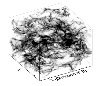
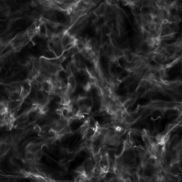
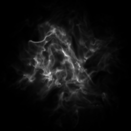
Figure 1.— Top: 3D density rendering of a $512^{3}$ MHD simulation where ${\cal M}_{s}$=10 (highly turbulent) and ${\cal M}_{A}$=0.7 (high magnetization), Model #2 from Table 1. The mean magnetic field is applied along the x-direction for each simulation. Bottom: Visualizations of compressed 2D column density (left) and cloud bounded column density (right). Each is created along the line of sight parallel to the mean magnetic field.

The top of Figure 1 presents a 3D density rendering of simulation #2 (Table 1) where ${\cal M}_{s}$=10 and ${\cal M}_{A}$=0.7. The x and y axes are labeled on the figure with the mean magnetic field ($<$B$>$) parallel to the x direction. The bottom displays, for the same simulation, a column density (left) and the same column density convolved with a radially decreasing Gaussian function in order to create the effect of cloud-like boundaries. See section 5 for descriptions of column density construction.

4. Tsallis Fit of Density, Velocity, and Magnetic Field

For the first portion of our analysis we investigate Tsallis fits of PDFs of 3D density and the three directional components of magnetic field and velocity. We fit the Tsallis distribution to incremental PDFs (see section 2) using the Levenberg-Marquardt algorithm (Levenberg 1944; Marquardt 1963), for spatial separations (lag) 1, 2, 4, 8, 16, 32, 64, and 128 pixels (up to 1.5 times smaller then the injection scale). Fits and PDFs are shown in Figure 2 (symbols are the data from the simulations, lines represent the Tsallis fit). Increasing lags are displayed vertically on the same logarithmic vertical scale. We only present magnetic and velocity fields directed along the mean magnetic field. EL10 saw no strong variation with LOS orientation for magnetic and velocity fields, which we confirm. PDFs of perpendicular components are therefore omitted from the figure.

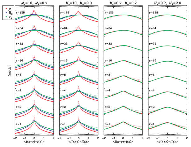
Figure 2.— PDFs of 3D density and components of velocity and magnetic field parallel to the mean magnetic field (red, green, and blue line respectively). Panels show four different simulations ${\cal M}_{s}$=10 ${\cal M}_{A}$=0.7, ${\cal M}_{s}$=10 ${\cal M}_{A}$=2.0, ${\cal M}_{s}$=0.7 ${\cal M}_{A}$=0.7, and ${\cal M}_{s}$=0.7 ${\cal M}_{A}$=2.0 (left to right). PDFs of larger lags are displayed vertically on the same scale for each simulation. Y-axis is logarithmic. Velocity and magnetic field produced similar PDF perpendicular to the mean magnetic field.

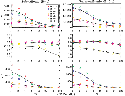
Figure 3.— From top to bottom, fit parameters $a$ (amplitude of fit), $q$ (related to fitting tails of PDF), and $w$ (PDF width plotted as $w^{-2}$) are displayed vs spatial lag for all 14 simulations showing 3D density. The left and right columns correspond to sub- and super-Alfvénic simulations respectively. Three solid lines are over-plotted for $a$ and $w^{-2}$ averaging the highly supersonic (${\cal M}_{s}$=10, 7, 6), mid supersonic (${\cal M}_{s}$=4, 3), and subsonic (${\cal M}_{s}$=0.7, 0.1) simulations. Two solid lines are over-plotted for the $q$ parameter averaging the supersonic (${\cal M}_{s}$=10, 7, 6, 4, 3) and subsonic (${\cal M}_{s}$=0.7, 0.1) simulations. Parameters $a$ and $w^{-2}$ show significant sensitivities to ${\cal M}_{s}$ and ${\cal M}_{A}$ (note scale between left and right panels). Parameter $q$ is only slightly sensitive to the simulation’s compressibility. Errors are generally less than 25$\%$, 20$\%$, and 40$\%$ for $a$, $q$, and $w^{-2}$ respectively. Error bars are omitted for clarity.

Figure 2 presents PDFs (and their corresponding Tsallis fits) of 3D density and components of velocity and magnetic field parallel to the mean magnetic field (red, green and blue lines respectively). Panels show four different simulations ${\cal M}_{s}$=10 ${\cal M}_{A}$=0.7, ${\cal M}_{s}$=10 ${\cal M}_{A}$=2.0, ${\cal M}_{s}$=0.7 ${\cal M}_{A}$=0.7, and ${\cal M}_{s}$=0.7 ${\cal M}_{A}$=2.0 (left to right). Visual analysis of these figures shows tightly correlated fits with only slight deviation near the tails of the PDFs (y-axis is logarithmic). Three outstanding trends can be seen across the simulations. First, is the increase in Gaussianity as ${\cal M}_{s}$ decreases (turbulence becomes subsonic). For supersonic turbulence, density PDFs are highly kurtotic. This corresponds to a higher probability that $\rho(x+r)-\rho(x)=0$ due to shock filaments causing central spikes of in PDFs increasing their kurtosis (agrees with trends seen in EL10 and Burlaga & Viñas 2004b). The second trend is the increase in Gaussianity as the lag increases. At low lags density, magnetic field, and velocity have higher probabilities of being near the mean value (here normalized to zero). This type of behavior is congruent with the results of Falgarone et al.(1994) which analyzed the skewness and kurtosis of PDFs of varying scales. In the case of subsonic turbulence, the PDFs of density look very similar to PDFs of velocity and magnetic field for high lags. Third, there is an increase in PDF kurtosis for density, velocity, and magnetic field for simulations of a high magnetic field (see the first and second panel of Figure 2 for small lags). Magnetization plays an intimate role in the development of turbulence and density enhancements and this affect can be attributed to field freeze-in. In the following subsections we will further describe the 3D quantities and their fits individually.

4.1. 3D Density

From top to bottom, Figure 3 displays fit parameters $a$, $q$, and $w$ (plotted as $w^{-2}$) versus the spatial lag for 3D density for all 14 simulations. The figure is separated on the left and right corresponding to sub- and super-Alfvénic Mach number simulations respectively. The top panels display parameter $a$ (corresponding the amplitude) and shows a strong sensitivity to the degree of sonic number. To emphasize this fact we break our simulations up into three categories; highly supersonic (${\cal M}_{s}$=10, 7, 6), mildly supersonic (${\cal M}_{s}$=4, 3), and subsonic (${\cal M}_{s}$=0.7, 0.1). A solid line is plotted through each subgroup’s average value at each lag. Attention to the difference in scale between the right and left panel shows a sensitivity to ${\cal M}_{A}$ as well.

Errors in the fit parameters are calculated from the standard deviation about each subgroup’s mean (i.e. highly supersonic, mildly supersonic, subsonic) for each lag.  Error bars are omitted from Figure 3 for clarity but are displayed in Figure 4 for $w^{-2}$.

The $a$ parameter has a percent error generally $<$ 25$\%$ but reaches a maximum of 56$\%$ for simulation ${\cal M}_{s}$=3.0 ${\cal M}_{A}$=2.0 (square symbol) at a lag of 1 pixel. The deviation from the mean mildly supersonic value is not large compared to the supersonic group but the lower numerical values produce a higher percent error. This error drops off significantly with increasing lag. This is to be expected for simulations since at low lags we are in the range of numerical dissipation. Super-Alfvénic errors all fall below 20$\%$.

In the middle panels, $q$ (related to the PDF’s tails) shows a slight sensitivity to the simulations compressibility and no magnetic sensitivity. For $q$ we break the simulations up into only supersonic (${\cal M}_{s}$=10, 7, 6, 4, 3) and subsonic (${\cal M}_{s}$=0.7, 0.1) and plot a solid line through their average values. The minimal variation in $q$ between simulations results in low errors that are below a 20$\%$ for each lag.

Parameter $w$, or width, displayed in the bottom panels of Figure 3 is presented as the fit value $w^{-2}$ as it appears in Equation (1) for convenience and clarity of representation. As with $a$, we plot solid lines of the average of highly super-, mildly super-, and subsonic simulations showing the same sensitivity to ${\cal M}_{s}$ although to a lesser degree. Both subsonic simulations lie along the lag (x) axis. The most outstanding trend seen in $w$ is its sensitivity to ${\cal M}_{A}$. Taking note of the large difference in scales between sub- and super-Alfvénic panels shows elevated values for simulations with high magnetic fields. Figure 4 summarizes this sensitivity displaying the sub- and super-Alfvénic versions of two highly supersonic (${\cal M}_{s}$=10, 7), one mildly supersonic (${\cal M}_{s}$=4), and one subsonic (${\cal M}_{s}$=0.7) simulation. For each ${\cal M}_{s}$, the sub-Alfvénic ($B_{\mathrm{ext}}$=1.0) simulation produces a $w^{-2}$ value $\geq$ 2 times its super-Alfvénic counter part at lag = 1 pixel.

Errors for $w^{-2}$ are the highest of the three parameters due to it large deviation between simulations. Generally the errors are $<$ 40$\%$ but peak at 160$\%$ for the ${\cal M}_{s}$=3.0 ${\cal M}_{A}$=2.0 simulation (filled circle) at 1 pixel lag. This is mainly due to its $<$ 1 value. Even with these significant errors, the differences between sub- and super-Alfénic turbulence is apparent.

Aside from the values of $a$, $q$, and $w$, the general shape of all three shows trends toward ${\cal M}_{s}$. Both $a$ and $w^{-2}$ show relatively consistent values over lag for subsonic simulations while supersonic simulations show steep decreasing slopes.

Figure 4.— An enlarged version of Figure 3’s bottom panel with ${\cal M}_{s}$= 10, 7, 4, 0.7 (top left to bottom right respectively). Sub-Alfvénic simulations are denoted with red diamonds while super-Alfvénic simulations are denoted with blue triangles. Both super- and sub-sonic simulations show larger $w^{-2}$ for high magnetization. Error bars are calculated from the standard deviation of the mean of each ${\cal M}_{s}$ group (highly supersonic, mildly supersonic, subsonic) at each lag.

4.2. 3D Velocity and Magnetic Field

The analysis of velocity is more directly related to investigations of turbulence than density and is particularly important in regards to Solar Wind measurements. Tsallis provides excellent fits to our velocity PDFs and also shows dependencies on Mach numbers, although the Tsallis fit parameters show decreased sensitivities to ${\cal M}_{s}$ and ${\cal M}_{A}$ compared to the density analysis.

The top panels of Figure 5 displays $w^{-2}$ for sub- and super-Alfvénic simulations on the left and right respectively for the component of velocity along the mean magnetic field (x-direction). Solid lines represent the average values of highly super-, mildly super-, and sub sonic simulations at each lag (for top and bottom panels). A small sensitivity to ${\cal M}_{s}$ can be seen with increased values for more turbulent simulations. The sensitivity to ${\cal M}_{A}$ is most predominant parallel to $<$B$>$ (which is the LOS shown in this figure) where there is a near factor of 2 increase in $w^{-2}$. Perpendicular to $<$B$>$, the increase is $\leq 50\%$. For sub-Alfvénic simulations ($B_{\mathrm{ext}}$=1) a $\sim$20% increase in $w^{-2}$ is seen for velocity along $<$B$>$ while no preferred direction is seen for super-Alfvénic simulations.

We do not show figures for $a$ and $q$ as they displayed less sensitivity to Mach numbers then did $w^{-2}$. Generally for velocity, the $a$ parameter displays a very small sensitivity to compressibility and the values for all simulations span a limited range. Compared to 3D density, velocity exhibits a two order of magnitude decrease in standard deviation for small lags. A slight increase in $a$ can be seen for velocity of highly magnetized simulations along the mean magnetic field (x direction) but no similar relationship is seen for velocity perpendicular to $<$B$>$. Fit parameter $q$ is even less descriptive, with no significant Mach number dependencies. $w^{-2}$ is the most sensitive to ${\cal M}_{s}$ and ${\cal M}_{A}$ maintaining the same trends seen in density but on a fraction of the scale.

Analysis of directional magnetic field strength is shown in the bottom of Figure 5 for $w^{-2}$. Tsallis fits the PDFs of magnetic field well. Parameter $w^{-2}$ displays a sensitivity to the ${\cal M}_{s}$ number of simulations of a given ${\cal M}_{A}$ as seen in the bottom panels of Figure 5 for the magnetic field parallel to $<$B$>$. In the presented figures $w^{-2}$ has a similar value for high and low ${\cal M}_{A}$ but along other lines of sight the relationship between $w^{-2}$ values and increased magnetization generally does not hold. However, this may be useful for determining mean field direction in the ISM. Similar to velocity, we find that $a$ and $q$ are not as useful as $w$ in terms of describing Mach numbers with component velocity and magnetic field, and hence we omit the Figures. Parameter $a$ shows a very small sensitivity to compressibility while $q$ shows no significant variation for any simulation.

Errors analysis for the fit parameters of velocity and magnetic field are carried out in the same manner as density (calculating the standard deviation of each ${\cal M}_{s}$ subgroup at each lag). Velocity along the mean magnetic field has fit errors consistently $<$ 18$\%$ for all lags and simulations. Magnetic field along the same LOS has similarly low errors ($<$ 20$\%$) with the exclusion of the sub-Alfvénic ($B_{\mathrm{ext}}$=1) ${\cal M}_{s}$=4 & 3 simulations (triangles and squares respectively) which reach 43$\%$ and 109$\%$ error respectively. One should keep in mind, however, that these measurements are done for one LOS as there are significant variations in the trends of velocity and magnetic field depending on the orientation.

The behavior of Tsallis fits to PDF increments of density, velocity, and magnetic field is in agreement with results found in EL10 at higher resolution with a larger parameter range. Our analysis of spatial variations provides insight into the underlying physics of MHD turbulence, where as the analysis of temporal variations of velocity and magnetic field in solar wind observations well described the multiphase structure of this phenomenon (Burlaga & Viñas 2004a, 2004b, 2005a, 2005b, 2006; Burlaga, Ness, & Acuñas 2006, 2007, 2009; Burlaga, Viñas, & Wang 2007). In the latter a time scale, $\tau_{m}$, (opposed to spatial scale $r$) is used to describe incremental fluctuations by $(B(t+\tau_{m})-B(t))$.

Figure 5.— Top: Fit parameter $w^{-2}$ for the velocity component parallel to the mean magnetic field for 14 simulations. Sub- and super-Alfvénic simulations are presented on the left and right respectively. Three solid lines are over-plotted averaging the super, trans, and subsonic simulations. Bottom: Fit parameter $w^{-2}$ for the magnetic field strength parallel to the mean magnetic field for 12 simulations. Three solid lines are over-plotted averaging the super, trans, and subsonic simulations. Errors for $\textbf{V}_{x}$ are all $<$ 18$\%$. Errors for $\textbf{B}_{x}$ are all $<$ 20$\%$, excluding mildly subsonic (${\cal M}_{s}$=4 & 3) sub-Alfvénic ($B_{\mathrm{ext}}$=1) simulations.

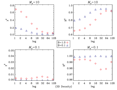
Figure 6.— $\chi^{2}$ and $R^{2}$ versus lag on the left and right respectively for 3D density simulations. The sub- and super-Alfvénic simulations are over plotted (red diamonds and blue triangles respectively) for ${\cal M}_{s}$=10 (top) and ${\cal M}_{A}$=0.1 (bottom). Tightest fits are obtained for medium lags for low magnetization and low turbulence. Largest deviations are seen for sub-Alfvénic supersonic simulations at small lags (in the dissipation range).

4.3. Quality of Fits

In order to characterize the quality of our fits and reliability of results, we calculate the Pearson’s $\chi^{2}$ and coefficient of determination, $R^{2}$, for our Tsallis PDF fits presented in Equations (5) and (6) below.

$$\chi^{2}=\sum\limits_{i=1}^{n}\frac{(y_{i}-f_{i})^{2}}{f_{i}},$$ (5)

$$R^{2}=1-\sum\limits_{i=1}^{n}\frac{(y_{i}-f_{i})^{2}}{(y_{i}-\bar{y})^{2}},$$ (6)

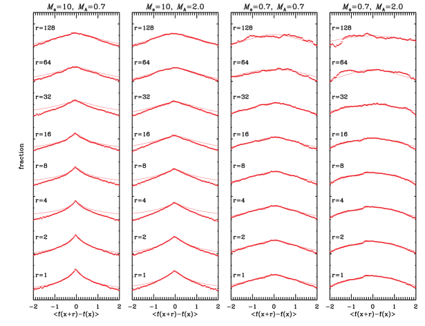
Figure 7.— PDFs of column density of four simulations with LOS averaged parallel to the mean magnetic field. From left to right, panels show ${\cal M}_{s}$=10 ${\cal M}_{A}$=0.7, ${\cal M}_{s}$=10 ${\cal M}_{A}$=2.0, ${\cal M}_{s}$=0.7 ${\cal M}_{A}$=0.7, and ${\cal M}_{s}$=0.7 ${\cal M}_{A}$=2.0. Column density made perpendicular to the mean magnetic field produced similar PDFs. Gaussianity of PDFs begins to degrade at high lags for subsonic simulations (top right)

In these equations, $y$ represents the observed PDF and $f$ is the Tsallis fit. Each measurement describes the accuracy of the fit. $\chi^{2}$ approaches zero for perfect fits while $R^{2}$ approaches one. In general, the Tsallis function will fit PDFs of density, column density, magnetic field, and velocity with a $\chi^{2}$$\leq$0.1 and a $R^{2}$$\geq$0.85 resulting in tightly correlated fits for the 100 degrees of freedom (number of bins in PDF histogram). Figure 6 displays the $\chi^{2}$ and $R^{2}$ for the sub- and super-Alfvénic counterparts of our most turbulent (top) and least turbulent 3D density simulations (bottom). From these plots we find that the best fits are seen for super-Alfvénic, subsonic simulations for lags greater than 16 pixels. Due to the kurtotic nature of high turbulence, low lag PDFs are difficult for Tsallis to fit at the central peak (see Figure 2, right panel, bottom). In these extreme cases (${\cal M}_{s}$=10, ${\cal M}_{A}$=0.7) values of $\chi^{2}$=0.67 and $R^{2}$=0.61 are obtained.

The low lag regimes are in the dissipation range of the turbulence, and Tsallis seems to have a difficult time fitting turbulence on scales sampling either the dissipation range or the injection scale. Despite these difficulties at low (or high) lag, Tsallis still can prove itself useful for characterizing turbulence. For example, if one is in the dissipation range of turbulence (i.e. at scales similar to our lags less then 32 pixels), then these “goodness of fit tests” can also be used to determine what type of turbulence is present. Subsonic and super-Alfvénic turbulence both are better fit with the Tsallis distribution at low lags then supersonic or sub-Alfvénic turbulence. At higher lags the fit quality converges as we enter the inertial range of turbulence. These fit tests should not only be preformed to test fit quality but could also be used as an additional test of the Mach number range in a given data set.

An alternative source of potential error in our analysis is the quality of PDFs at large lags. Not only are these lags on the upward scale of the inertial range, but also are subjected to degraded resolution. These resolution effects can be seen particularly in the case of the column density, which are 2D quantities discussed in the next section. The inspection of Figure 8 shows fits becoming less tight at large lags. This manifests as “jumps” in the fits parameters which can be seen in the subsonic case in Figure 9. This is the most extreme example of this trend but it is seen to some degree for every simulation at a large enough lag. In these cases the $\chi^{2}$ and $R^{2}$ remain constrained to the values stated above. We conclude that, for this analysis, our results are most stable for lags in the inertial range of turbulence and for lags at least 8 times smaller then the box size to provide enough sampling. This trend is consistent with the results seen using higher order moments to analyze the incremental PDFs.

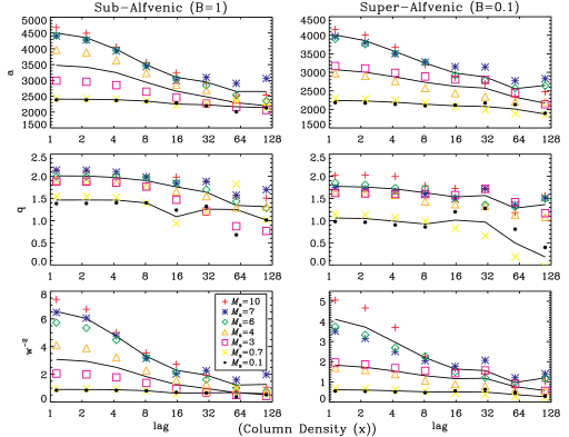
Figure 8.— From top to bottom fit parameters $a$ (amplitude of fit), $q$ (related to fitting tails of PDF), and $w$ (PDF width plotted as $w^{-2}$) are displayed vs spatial lag for all 14 simulations. Column density are LOS averaged parallel to the mean magnetic field. The left and right columns correspond to sub- and super-Alfvénic simulations respectively. Three solid lines are over-plotted for $a$ and $w^{-2}$ averaging the highly supersonic (${\cal M}_{s}$=10, 7, 6), transonic (${\cal M}_{s}$=4, 3), and subsonic (${\cal M}_{s}$=0.7, 0.1) simulations. Two solid lines are over-plotted for the $q$ parameter averaging the supersonic (${\cal M}_{s}$=10, 7, 6, 4, 3) and subsonic (${\cal M}_{s}$=0.7, 0.1) simulations. Parameters $a$ and $w^{-2}$ show sensitivities to ${\cal M}_{s}$ and ${\cal M}_{A}$ (note scale between left and right columns). Parameter $q$ is only slightly sensitive to the simulation’s compressibility. Lags from 2 to 32 pixels provide the most consistent fit parameter errors where $a$, $q$, and $w^{-2}$ maintain errors $<$ 22$\%$, 35$\%$, and 24$\%$ respectively.

5. Tsallis Fit of 2D Column Density and PPV data

In section 4 we confirmed the results of EL10 using higher resolution simulations and a substantially larger parameter range. In addition, we demonstrate the sensitivity the $w$ (width) fit parameter has toward the Alfvénic Mach number. However, observations of the ISM do not provide direct 3D information of density. Combining density and velocity along the line-of-sight (LOS) provides a 3D position-position-velocity (PPV) cube, however these types of data cubes can almost never be reliably interpreted as having a one-to-one correspondence with an actual 3D volume density. Considering the difficulties of obtaining direct 3D ISM information, a study of Tsallis statistics on observables such as column density and PPV data is necessary.

5.1. Column Density

We create synthetic 2D column density maps perpendicular and parallel to the mean magnetic field for all 14 of our simulations by averaging the 3D density cubes along a given line of sight. We assume the emitting gas is optically thin and that the emissivity is linearly proportional to density (such as in the case of HI). An example is presented in Figure 1 (bottom left). Using the same method described in the section 2, PDFs are created using spatial lags (increments) in two directions which are then fit using the Tsallis function.

Figure 7 displays the distributions and fits for 4 simulated column densities created parallel to the mean magnetic field. The 4 simulations we show here are divided into panels: ${\cal M}_{s}$=10 ${\cal M}_{A}$=0.7, ${\cal M}_{s}$=10 ${\cal M}_{A}$=2.0, ${\cal M}_{s}$=0.7 ${\cal M}_{A}$=0.7, and ${\cal M}_{s}$=0.7 ${\cal M}_{A}$=2.0 (left to right). This is analogous to the arrangement in Figure 2. While there is an overall decrease in kurtosis of the column density PDFs compared to 3D density, the same three trends are still apparent. PDFs become more Gaussian with decreased ${\cal M}_{s}$, Gaussianity increases with lag for supersonic cases, and Gaussianity increases with ${\cal M}_{A}$. A trend not seen in the 3D case is that subsonic PDFs become less smooth at high lags. This is due to the decrease in resolution going from 3D to 2D. EL10 also observed this trend with their subsonic PDFs.

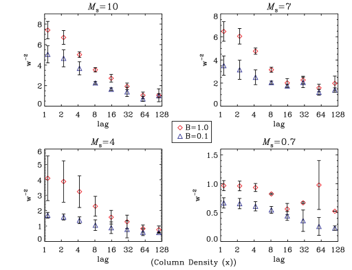
Figure 9.— An enlarged version Figure 8’s bottom panel with ${\cal M}_{s}$= 10, 7, 4, 0.7 (top left to bottom right respectively). High magnetization is denoted with red diamonds and low magnetization is denoted with blue triangles. Both super- and subsonic simulations show larger $w^{-2}$ for high magnetization. Error bars are calculated from the standard deviation of the mean of each ${\cal M}_{s}$ group (highly supersonic, mildly supersonic, subsonic) at each lag.

Figure 8 displays the fit parameters $a$, $q$, and $w^{-2}$ from top to bottom for all 14 column density simulations created along the x direction (parallel to $<$B$>$). Each parameter is divided into two panels with sub-Alfvénic and super-Alfvénic simulations on the left and right respectively. The $a$ parameter (top panels) is presented with three over-plotted lines, averaging the super-, mildly super-, and subsonic simulations. Again, a strong sensitivity to ${\cal M}_{s}$ is seen both in the value and the shape of the fit over spatial scale. The sensitivity to ${\cal M}_{A}$ is less prevalent than in 3D density.

Errors for column density fit parameters are calculated in the same manner as 3D density by measuring the standard deviation of each ${\cal M}_{s}$ subgroup at each lag. The $a$ parameter achieves $<$ 23$\%$ errors for each lag and simulation reaching the lowest errors ($<$ 5$\%$) at lags between 16 and 64 pixels. As in density, error bars are excluded from Figure 8 for clarity but displayed in Figure 9 for $w^{-2}$.

Parameter $q$ (middle panels) is presented with averaging super- and subsonic lines showing a slight sensitivity to ${\cal M}_{s}$ and no coherent sensitivity to ${\cal M}_{A}$. Errors for $q$ are generally less than 30$\%$ but begin to reach percent errors greater than 100$\%$ for subsonic simulations at lags greater than 34 pixels due to random variations. Inspection of the right panel of Figure 7 shows that this is consistent with when the PDF start to become nonuniform.

The $w$ parameter (bottom panels), here plotted as $w^{-2}$, shows both a strong sensitivity to ${\cal M}_{s}$ and ${\cal M}_{A}$. Highly super-, mildly super-, and subsonic averaging lines are over-plotted which emphasize that values of $w^{-2}$ are affected by ${\cal M}_{s}$. Errors for $w^{-2}$ are $<$ 25$\%$ for lags of 2 to 32 pixels. Maximum errors reach values of 70$\%$ at a 1 pixel lag and 60$\%$ error at lags greater than 64 pixels. Interestingly, as in EL10, subsonic column densities shows a more random behavior at larger lags due to low resolution and low density contrasts.

Figure 9 summarizes $w$’s Alfvénic sensitivity by displaying the sub- and super-Alfvénic versions of two highly supersonic (${\cal M}_{s}$=10, 7), one mildly supersonic (${\cal M}_{s}$=4), and one subsonic (${\cal M}_{s}$=0.7) simulation. In each case, the simulation having the higher magnetic field results in a higher $w^{-2}$ value. Although the degree to which $w^{-2}$ is elevated is less than for 3D density, a strong direct correlation remains. Subsonic trends become less smooth at lag=32 pixels, which is $\approx$ 6.4 times smaller then the injection scale. We may conclude that the column density has a stronger dependency on lag then in the 3D cases, especially for subsonic turbulence.

We analyze fit parameters from column densities created along the y and z axes (i.e. perpendicular to the mean magnetic field) and while there were slight variations in the fits, sensitivities to Alfvén and sonic Mach numbers were still observed. No discernible trend to detect magnetic LOS orientation was seen.

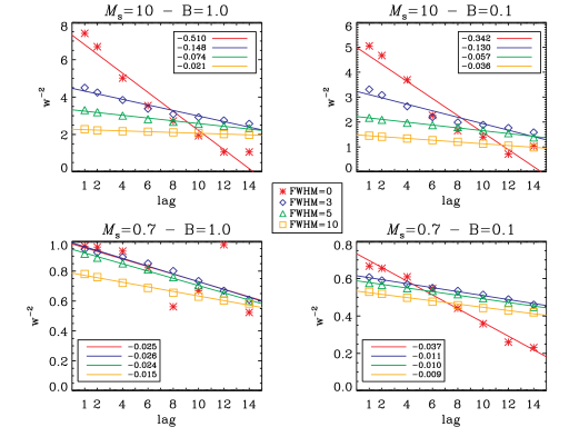
Figure 10.— Fit parameter $w^{-2}$ for ${\cal M}_{s}$= 10 (top), and 0.7 (bottom) with sub- and super-Alfvénic simulations on the left and right respectively. The original and smoothed data are over-plotted. Least squares linear fits are over plotted in the same color. The enclosed legends displays the slope of the respective linear fits. The central legend provide the FWHM of smoothing (FWHM=0 is unsmoothed). Increased smoothing results in decreased values and shallower slopes.

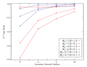
Figure 11.— Slope of $w^{-2}$ (width) for the sub- and super-Alfvénic versions of the ${\cal M}_{s}$=7, 4, and 0.7 simulations plotted against the smoothing degree in FWHM size. High and low magnetization are presented in red and blue respectively. Supersonic simulations are more dramatically affected than subsonic as turbulent density enhancements are smoothed out.

5.1.1 Effects of Smoothing

While the analysis simulated column density maps shows the strength of Tsallis statistics in describing turbulent characteristics, analogous observational column density data do not have pencil thin beam resolution. To address this issue, we experiment with smoothing our column densities to different degrees to determine the role degradation of resolution plays in distributions and fit sensitivities. Using a Gaussian smoothing kernel, we degrade our column density simulations with a full-width-half-maximum (FWHM) of 3, 5, and 10 pixels.

In an effort to characterize the effects of smoothing we increase our lag resolution by creating the same number of distributions over a smaller range of lags. Figure 10 presents the the original and smoothed fit parameter $w^{-2}$ for sub- and super-Alfvénic simulations versions of simulations ${\cal M}_{s}$=10 and 0.7 from top left to bottom right respectively. While we investigated the effects of smoothing on all three fit parameters, we only present $w^{-2}$ as the effects on $q$ and $a$ are similar. In order to characterize how the slope of the Tsallis parameters vs. lag change with increasing smoothing a least squares linear fit is applied to each scenario with the slopes displayed in the respective legends. The red stars denote the non-smoothed case for comparison. From this figure it is clear that increased smoothing lowers the values of $w^{-2}$ for each lag and its overall slope. These effects are present across all simulations. While the supersonic (top row) simulations show smooth monotonic trends for both smoothed and pencil beam data, subsonic simulations (bottom row) shows very bumpy trends for the case where no smoothing is introduced (red stars and line) especially as lag increases. However, as we introduce smoothing, the trends become highly monotonic, even for the case of FWHM=3 pixels. Applying Tsallis fits to incremental PDFs while varying the level of smoothing will act as an additional tool to characterize turbulent parameters through the overall change in slope.

Figure 11 provides a summary of the effect smoothing has on the slope of $w^{-2}$ by plotting it against the smoothing degree. Simulations of the same sonic number are shown with the same symbol while the color corresponds to the previously used color scheme (red being $B_{\mathrm{ext}}$=1, sub-Alfvénic and blue being $B_{\mathrm{ext}}$=0.1, super-Alfvénic). We see that increased smoothing flattens the $w^{-2}$-lag slope. A sensitivity to the ${\cal M}_{A}$ is still present in both slope and value in every smoothing cases (note scale between sub- and super-Alfvénic simulations in Figure 10). High sonic Mach number simulations show slopes that are the most altered as smoothing is increased. This is due to shock density enhancements being smoothed out. However, the supersonic cases show larger variation with differing ${\cal M}_{A}$ then their subsonic counterparts. This leads us to believe that one can more easily tell the magnetization strength of supersonic gas from Tsallis fits. Increasing the smoothing does not affect the subsonic cases, as these simulations already have Gaussian distributions and have no peak density enhancements from shocks to smooth out.

Parameter $a$ was affected by smoothing in the exact same way $w^{-2}$. Values and slopes decreased with increased smoothing. Plots are excluded for brevity but both $a$ and $w$ could be explored with increasing smoothing to put estimates on turbulence. The $q$ parameter saw little deviations due to smoothing and a slightly weakened ${\cal M}_{s}$ sensitivity.

Fit parameter errors for our smoothing discussing can be considered to decrease with smoothing from their unsmoothed values (quoted in the previous section) as differences in ${\cal M}_{s}$ sub groups of simulations become washed out in parameter space.

5.1.2 Artificial Noise

While analysis using Tsallis statistics is very adept at providing turbulence parameters when smoothing is applied to column density maps, more pressing maybe the issue of noise. One may not expect noise to affect results at larger lags however, noise may make it challenging to distinguish trends on smaller scales where the difference between our simulations is prominent. It is our intent in this subsection to test the effectiveness of this statistical tool with the addition of noise, determine our confidence range between trends with noise and with no noise, and explore which lags are most affected by the addition of noise. In order to achieve this end we add random Gaussian noise to our column density maps. We do this by setting a given average signal-to-noise (SNR) ratio and scaling the power of the noise and signal to match this SNR. We look at column density integrated parallel to the mean magnetic field with average SNR of 400, 200, 100, 50, 20 and unity.

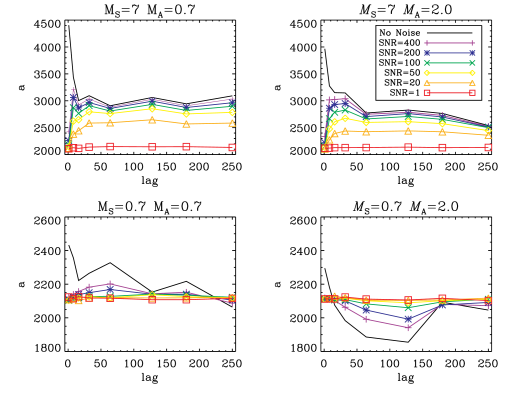
Figure 12.— Fit parameter $a$ for 4 simulations (sub and super-Alfvénic of simulations ${\cal M}_{s}$=7, 0.7) with varying levels of noise (see legend). Small amounts of noise drastically lower small lags values and has an overall smoothing affect. Increasing noise lowers $a$’s sensitivity to ${\cal M}_{s}$ and ${\cal M}_{A}$.

Figure 13.— Fit parameter $w^{-2}$ for 4 simulations (sub and super-Alfvénic of simulations ${\cal M}_{s}$=7, 0.7) with varying levels of noise (see legend). Small amounts of noise drastically lower small lags values and has an overall smoothing affect. Increasing noise lowers $w^{-2}$’s sensitivity to ${\cal M}_{s}$ and ${\cal M}_{A}$.

The addition of noise on the column density PDFs has a general smoothing effect toward Gaussianity (PDFs not shown). This is to be expected as the noise added to the column density is Gaussian white noise. Figures 12 and 13 illustrate the effects of noise for the parameters $a$ and $w^{-2}$ respectively for four simulations with given sonic Mach numbers of ${\cal M}_{s}$= 7.0 and 0.7 and Alfvénic number ${\cal M}_{A}$= 2.0 and 0.7. From these figures it is clear that the smaller spacial lags (lags = 1 - 32 pixels) are highly affected by the addition of noise. The noise injected simulations (lines with colors and symbols) do not converge to their no-noise counter part (shown as a solid black line) until lag $\sim$20 pixels. At around lag 20, simulations with SNR greater than 50 show similar shaped curves to the no-noise case. As the SNR decreases, the values of $w$ and $a$ both decrease for the supersonic case. The subsonic case shows a more pronounced non-monotonic behavior. In all cases above SNR of 20, the sub-Alfvénic supersonic turbulence shows heightened values of $a$ and $w^{-2}$. The sonic number between these two simulations can be determined within 1.5 $\sigma$ confidence at SNR 20 and above. At SNR of unity it is impossible to distinguish between either sonic or Alfvénic numbers, which is to be expected.

A SNR greater than 100 is sufficient for showing differences in $w^{-2}$ and $a$ between sub- and super-Alfvénic simulations, with sub-Alfvénic producing larger values. In the case of supersonic turbulence a SNR of 20 is generally sufficient to discern between sub- and super-Alfvénic gas using Tsallis fit parameters with 1.5$\sigma$ confidence for all lags. While this is promising that all pixel scales show statistically significant differences, the shape of the $w^{-2}$ or $a$ curve vs. lag converges to non-noise levels only for lag $\sim$20 pixels and therefore, small lags may not be as reliable as larger lags in the presence of low SNR. Subsonic cases can distinguish Alfvénic number with confident in the 1 $\sigma$ range at SNR 20 and greater for lags larger then 32 pixels.

5.1.3 Simulating Cloud Boundaries

Studies of the ISM frequently deal with both clouds-like objects as well as diffuse gas. While our simulations are most directly applicable to diffuse ISM, we can also study the effects the Tsallis fits will have on ISM gas with boundaries. An example of such a situation would be molecular clouds which have characteristic radially decreasing density values. To mimic this, we convolve our 3D density simulations with a spherical function which maintains the value inside a given radius R from the center and creates a Gaussian decay outside this radius. For our simulations we choose an R of 205, 90, and 10 pixels corresponding to 2.5, 6, and 51 times smaller than box size respectively. The cloud convolved 3D simulations are then averaged along a LOS creating a column density map as described in section 5.1. For reference a column density map with a radial decreasing Gaussian boundary starting at R=90 parallel to the mean magnetic field is presented in Figure 1 (bottom right) for simulation #2 (${\cal M}_{s}$=10, ${\cal M}_{A}$=0.7).

Figure 14.— From top to bottom fit parameters $a$ (amplitude of fit), $q$ (related to fitting tails of PDF), and $w$ (PDF width plotted as $w^{-2}$) are displayed vs spatial lag for all 14 simulated cloud bounded column density simulations created parallel to the mean magnetic field (R=205, 2.5 times smaller than cube and the scale of the turbulent energy injection). The left and right columns correspond to sub- and super-Alfvénic simulations respectively. Three solid lines are over-plotted for $a$ and $w^{-2}$ averaging the supersonic (${\cal M}_{s}$=10, 7, 6), transonic (${\cal M}_{s}$=4, 3), and subsonic (${\cal M}_{s}$=0.7, 0.1) simulations. Two solid lines are over-plotted for the $q$ parameter averaging the supersonic (${\cal M}_{s}$=10, 7, 6, 4, 3) and subsonic (${\cal M}_{s}$=0.7, 0.1) simulations. Parameters $a$ and $w^{-2}$ show sensitivities to ${\cal M}_{s}$ and ${\cal M}_{A}$ (note scale between left and right columns). Parameter $q$ is only slightly sensitive to the simulation’s compressibility. Lowest error are achieved for supersonic simulations at lags between 4 and 32 pixels where percent errors are below 44$\%$, 40$\%$, and 84$\%$ for $a$, $q$, and $w^{-2}$ respectively. Outside this constraint, error $>$ 150$\%$ for each parameter.

In general, a radially decreasing cloud boundary creates an increase in the kurtosis of the PDFs as compared with unbounded column density (not shown). This change comes from the increase in zero point values of $\rho(x+r)-\rho(x)=0$ as more contrast is created. At a radius of 205 pixels the PDFs are still fairly uniform and only see slight variations from Gaussianity for subsonic simulations and fits remain similar to those seen in Figure 7.

Figure 14 presents the $a$ (top), $q$ (middle) and $w^{-2}$ (bottom) fit parameters for the R=205 bounded simulations parallel to the mean magnetic field. As with 3D density and unbounded column density, sub- and super-Alfvénic simulations are presented on the left and right panels respectively. Three averaging lines are plotted through the highly super-, mildly super-, and subsonic simulations for $a$ and $w$, while $q$ has only super- and subsonic averaging lines. Sensitivities to ${\cal M}_{s}$ are still apparent throughout the $a$ and $w^{-2}$ fits values and slopes but emphasized more in sub-Alfvénic simulations. ${\cal M}_{A}$ remains strongly tied to $w$, as presented in Figure 15. In each scenario, the simulation containing a stronger magnetic field results in a $\geq$2 times higher value of $w^{-2}$. The $q$ parameter shows little effect from a radially decreasing boundary condition and still is only mildly affected by simulation compressibility.

Fit parameter errors of cloud bounded column densities shows similar trends to those seen in full resolution 2D density maps. Parameter $a$ maintains the lowest error from lag 2 to 32 pixels where errors remain $<$ 16$\%$. Outside this range, errors increase and reach a maximum error of 46$\%$ at the 1 pixel lag. $q$ achieves errors below 36$\%$ for most simulation lags excluding subsonic simulations and large lags. In this regime error reaches 90$\%$. Errors of the $w^{-2}$ parameter display similar trend as $q$ where errors below 50$\%$ are produced for mid range lags (4-32 pixels) and highly and mildly supersonic simulations. Errors reach $>$ 150$\%$ at small lags and subsonic simulations at high lags. This further confirms the trend that decreasing resolution has on the quality of fits and fit parameter values. Even as errors increase, the $w^{-2}$ parameter is still able to distinguish ${\cal M}_{A}$ within the error bars.

Similar to the incremental column density PDFs, our largest clouds proved well described by Tsallis statistics. However, the decrease in cloud size greatly affects the PDFs and the ability of the Tsallis function to fit them. For example, in the case of our smallest cloud (R=50 pixels), the PDF and fit for simulation #2 (${\cal M}_{s}$=10, ${\cal M}_{A}$=0.7) at even our largest lag (128 pixels, not shown), is extremely kurtotic and skewed to negative values. This is due to radially decreasing density, the value of $\rho(x+r)-\rho(x)$ is in general $>$ 0 for three out of the four directional calculations (+x, -x, +y, -y). Tsallis is a symmetric function about $\rho(x+r)-\rho(x)=0$ and this skewness of the PDF prevents tight fits. While quality of the fit is no longer intact, the relative amplitudes and widths change with lag, ${\cal M}_{s}$, and ${\cal M}_{A}$.

Cloud convolved column densities with LOS perpendicular to the mean magnetic field were also analyzed and showed the same trends and no discernible correlation with the LOS orientation.

Figure 15.— An enlarged version of Figure 14’s bottom panels for ${\cal M}_{s}$ = 10, 7, 4, and 0.7. Sub- and super-Alfvénic simulations are over-plotted in red diamonds and blue triangles respectively. Both Super- and Sub-sonic cases have elevated values for high magnetization. Error bars are calculated from the standard deviation of the mean of each ${\cal M}_{s}$ group (highly supersonic, mildly supersonic, subsonic) at each lag.

5.2. PPV Cubes

The application of Tsallis statistics has proven itself to be a useful tool for exploring a wide parameter range of sonic and Alfvénic Mach numbers in density and column density data. However, while density fluctuations are indeed useful for characterizing turbulence, more appropriate is the use of velocity information. We test the usefulness of Tsallis PDF fits on Position-Position-Velocity (PPV) data in order to see if additional information is provided by including the velocity axis. We create synthetic PPV cubes of our full simulation range using density and velocity with LOS perpendicular to mean magnetic field. In order to test a variety of velocity resolutions we create PPV cubes with velocity widths of 0.15 ($\sim$30 channels), 0.07 ($\sim$60 channels), and 0.007 ($\sim$600 channels). Units remain scale free.

Figure 16 presents $w^{-2}$ vs. lag for the sub- and super-Alfvénic versions of the ${\cal M}_{s}$=10, 4, and 0.7 simulations from top to bottom respectively. Each panel has the three velocity resolutions over-plotted for comparison. Low, middle, and high resolutions are represented by the circle, diamond, and triangle respectively. Within each resolution, red symbols correspond to sub-Alfvénic ($B_{\mathrm{ext}}$=1.0) while blue corresponds to super-Alfvénic ($B_{\mathrm{ext}}$=0.1). All three panels display a common trend of decreasing $w^{-2}$ value as the velocity resolution increases (width of the velocity channels decreases). Also, it is clear that the $w$ parameter is sensitive to the ${\cal M}_{A}$ number for PPV simulations and produces elevated values for simulations with high magnetization.

The general shape of $w^{-2}$ over increasing lags is distinctly different for PPV data than in density, velocity, or magnetic field. The PDFs, and therefore fit parameters are more consistent with lag variations and produce smoother trends. This alternative trend is only seen in supersonic PPV data while values of $w^{-2}$ for subsonic PPV data more closely resemble the trends seen in density analysis.

Parameter $a$ shows minimal variations to ${\cal M}_{A}$ or ${\cal M}_{s}$ for PPV simulations. Sensitivities to ${\cal M}_{s}$ are seen on a scale too small to be used observationally and there is no coherent relationship to ${\cal M}_{A}$. Similar to previous discussions $q$ only provides limited information on compressibility and none on ${\cal M}_{A}$.

It should be noted that during the distribution creation process, especially for high velocity resolutions, velocity channels with little emission were excluded. In addition, a majority of the small lag PDFs had a single multiple order of magnitude jump at the center of the distribution (where $\rho(x+r)-\rho(x)=0$). This point was excluded from the fitting process. This is simply due to the way the emission is spread over the channels in PPV with a Maxwellian velocity distribution. Most gas is near the mean velocity and a Gaussian decrease in emission is seen as one goes to the extreme minimum and maximum channel velocities.

Analysis of density distributions along the velocity axis for individual pixels were also analyzed. An attempt to fit these distributions with the Tsallis function proved ineffective. We find the distribution of density emission along velocity channels, especially for high turbulence, are highly skewed and irregular which is consistent with the findings of Falgarone et al. (1994). As Tsallis is a symmetric function it is not able to provide tight fits to these highly irregular and varying distributions.

Figure 16.— Parameter $w$ (PDF width plotted as $w^{-2}$) for ${\cal M}_{s}$= 10, 4, 0.7 from top to bottom respectively. Each panel plots the sub- and super-Alfvénic simulations for the three velocity channels (see legend). A sensitivity to ${\cal M}_{A}$ is seen in every case but more pronounces for high turbulence simulations and few velocity channels. Subsonic simulations shows trends that resemble density while supersonic simulations do not.

6. DISCUSSION

6.1. Summary and the Relation of Tsallis to Other ISM Statistics

We studied Tsallis statistics as a way to characterize MHD ISM turbulence. While we do not address the theoretical justification of the particular form of the fits predicted by the Equation (1), our study shows that this fit provides a very good correspondence with experimentally obtained distributions. We showed that the parameters that enter the Tsallis expression are dependent on the Sonic Mach (${\cal M}_{s}$) and Alfvénic Mach (${\cal M}_{A}$) numbers, confirming and extending the earlier claims of Esquivel & Lazarian (2010). In addition, we explored the differences in the dependencies of the fitting parameters on both ${\cal M}_{A}$, ${\cal M}_{s}$ and on the resolution. This allows one to find ${\cal M}_{s}$ and ${\cal M}_{A}$ independently. We also applied Tsallis statistics to PPV data, which, as far as we know, is the first time such a study has been undertaken.

Another important point that we address here is the influence of telescope resolution in the form of smoothing. This issue was largely omitted in our earlier publications, but our results show that the influence of the telescope beam may be important for observational studies. Not only does smoothing affect the statistics, but it could actually be a helpful addition to the statistical procedure to study Mach numbers. Indeed, telescope measurements introduce their own smoothing, which depends on the telescope resolution. As the injection scale of the turbulence is frequently not known, the given measurements of the parameters of the Tsallis statistics may not be straightforward to identify with the particular simulation. In this situation, additional smoothing can help to see to what parameters of turbulence the observed data corresponds to.

Burkhart et al. (2010) studied the Small Magellanic Cloud (SMC) to characterize the properties of turbulence in its individual parts. The same approach is applicable with Tsallis statistics. It is convenient to note, that one can gain information on regions turbulence or magnetization without knowing the precise resolution of the telescope. Our motivation for applying boundaries to our simulations was fueled by making Tsallis applicable to more compact objects, such as those that may be found in molecular clouds. Our results show clear tendencies to determine Mach number information from the Tsallis fitting parameters.

In addition, our study shows that the use of the full PPV data can bring additional advantages. For instance, the evolution of Tsallis parameters with is clearly different for subsonic and supersonic cases (see Figure 16) in PPV data.

We feel that the Tsallis fit provides useful way of studying turbulence, which should be implemented along with other techniques used previously (see Kowal, Lazarian, & Beresnyak 2007; Burkhart et al. 2009, 2010). We advocate an approach which combines the use of different techniques. For instance, the effect of the telescope beam smoothing depends on the ratio of the angular size of the turbulence energy scale in the object under study and the telescope resolution. The former can be obtained by studying the power spectra of turbulence.

While we are still searching for the basic approaches to study turbulence observationally, the successes in theoretical and numerical studies provide us with a reliable guidance for obtaining statistics of turbulence from observations. The development of the VCA and VCS techniques (see Lazarian & Pogosyan 2000, 2004, 2006, 2008, Chepurnov & Lazarian 2008) for instance, quantified how velocity and density create structures observed in the PPV. Results on the anisotropies of observational data statistics in the plane of the sky in Lazarian, Pogosyan & Esquivel (2002) and subsequent publications (Esquivel & Lazarian 2005) reveals strong dependencies on media magnetization. Kurtosis and skewness measures of the density (Kowal, Lazarian, & Beresnyak 2007; Burkhart et al. 2009) provide good insight mostly into the intensity of turbulence, i.e. its ${\cal M}_{s}$. Genus (see Lazarian 1999, Kim & Park 2007, Chepurnov et al. 2008) provides a measure of topology, while bispectrum (see Burkhart et al. 2009) provides insight into mode correlation and phase information of the turbulence. Additional information can be obtained by employing other tools, e.g. dendrograms (Rosolowsky et al. 2008, Goodman et al. 2009, Burkhart et al. 2011). At the same time the synergy of the simultaneous use of different techniques is still to be explored.

6.2. Relation of This Study to Previous Tsallis Work

In this paper we fit the Tsallis distribution function to PDFs of turbulence with little or no theoretical justification. Indeed, while the history of turbulence studies can be traced back to Kolmogorov (1941), turbulence studies have since taken many different directions. In this paper, we are particularly interested in characterizing magnetized turbulence in the ISM. The Tsallis distribution formalization comes from a different background, specifically the issue of quantities which are invariant in the Navier-Stokes equations at high Reynolds numbers and the assumption that the singularities due to the invariance distribute themselves multifractally in physical space. Much work has been done to address both the theoretical frame work and application of the Tsallis statistics to numerical and laboratory turbulence PDFs (see Tsallis 1999 and Arimitsu & Arimitsu (2000a, 2000b, 2001, 2002, 2003)). For example, in Arimitus & Arimitus 2003, the authors successfully fit the Tsallis distribution to PDFs of turbulence in three different laboratory experiments. Burlaga and collaborators successfully fit Tsallis to solar wind data (Burlaga, Viñas, & Wang 2009).

In this paper, we successfully fit Tsallis to our numerical magnetized ISM turbulence, even in the case of observable quantities such as column density and PPV emission cubes. In the case of the laboratory, space observations, and numerical experiments; the geometry of the system, the Reynolds numbers, and the type of turbulence in question, are all very different. Never-the-less, in all cases the Tsallis distribution provided good fits to the data. Motivated by these past studies, we applied the Tsallis function in an empirical way to determine the parameters of turbulence, and we direct the curious reader to the literature mentioned above for a more in depth treatment of the theoretical foundations of the Tsallis function. Also, our paper is motivated towards making Tsallis statistics useful for observational studies of turbulence, and in this case the discussion of multifractal theory is beyond our current scope. We do not attempt to justify or even test these ideas, but investigate to what degree the fit provided by the two parameter Tsallis formula corresponds to our numerical data.

6.3. The Issues of Numerical Resolution

While there is no doubt that substantial progress has been made in last decade in numerical simulations of turbulence, the community still has a long way to go in terms of achieving the resolution required to fully capture ISM physics. One issue in particular is the discrepancy between astrophysical values of Reynolds (Re) and magnetic Reynolds (Rm) and the numerical values. As a rule, astrophysical environments are turbulent and astrophysical turbulence is characterized by enormously large Re and Rm. For instance, the Rm number, which characterizes the degree of frozenness of magnetic field within eddies, may differ in astrophysical environments and numerical simulations by a factor larger than $10^{10}$. With these sorts of discrepancies in mind (which exist for all numerical codes that simulate turbulence), how are we able to justify our results?

There are several avenues to justify the independence of our results from Re and Rm values. The particular numerical code used here provides enough resolution to allow us to see the inertial range of turbulence. If turbulence is evolving along the inertial range it is self-similar, and the change in Re and Rm does not change the structure of the large scale motions which we study here. Indeed, according to the Lazarian & Vishniac (1999) model of turbulent reconnection (tested in Kowal et al. 2009), magnetic reconnection in a turbulent media depends on the large scale field wondering determined by large scale motions. Thus we do not expect the unresolved small scales to affect the physics of our simulations at large scales that we study. Keeping all of this in mind, we also tested our Tsallis fits at resolutions of $256^{3}$ and $512^{3}$ and found no deviation in how well Tsallis was able to both fit the PDFs and describe the turbulence in question.

7. CONCLUSIONS

In this paper we applied the Tsallis formalism to simulated diffuse ISM isothermal ideal MHD turbulence using incremental PDFs of density, velocity, and magnetic field. This method was also applied to simulated column densities with measures taken to duplicate observed measurements such as smoothing, noise, and radial decreasing cloud boundaries. The use of Tsallis statistics on PPV data was also explored. A summary of our findings is as follows:

• The Tsallis function is capable of well describing incremental PDFs of a wide range of simulated MHD density, velocity, and magnetic field with its three fit parameters $a$ (amplitude), $w$ (width), and $q$ (related to the PDF’s tails).

• For 3D density, fit parameters $a$, $q$, and $w^{-2}$ are sensitive to ${\cal M}_{s}$. $a$ and $w^{-2}$ show sensitivities to ${\cal M}_{A}$ with both displaying greater values for sub-Alfvénic simulations.

• Magnetic field and velocity show sensitivities to ${\cal M}_{s}$ and ${\cal M}_{A}$ but these are not as strong as density.

• PDFs of column density are equally well described by the Tsallis distribution. Fit parameters $a$, $q$, and $w^{-2}$ remain sensitive to ${\cal M}_{s}$. $a$ looses some of its magnetic sensitivity but $w^{-2}$ consistently produces elevated values for sub-Alfvénic simulations.

• The affect of degrading resolution lowers both $a$ and $w^{-2}$ vs. lag monotonically. Supersonic simulations are most affected by smoothing. $a$ and $w^{-2}$ remain sensitive to ${\cal M}_{s}$ and ${\cal M}_{A}$ for mild smoothing. $q$ looses ${\cal M}_{s}$ sensitivity with smoothing.

• The addition of smoothing at varying degrees acts as an additional method to constrain sonic Mach number through the analysis of the slope of parameters $a$ or $w^{-2}$ over lag.

• Noise has the largest affect on fit parameters. Small scale variations strongly alter the PDFs of low lags and the shape of the fit distributions. Sensitivities to ${\cal M}_{A}$ and ${\cal M}_{s}$ are still seen on smaller scales as the spatial lag increases.

• Radially deceasing cloud boundaries have little affect as long as a there are enough points inside providing good signal. As clouds become smaller, PDFs become more kurtotic and skewed preventing meaningful fits.

• PPV data was fit with Tsallis distribution excluding the zero point and parameter $w^{-2}$ showed sensitivities to ${\cal M}_{s}$ and ${\cal M}_{A}$.

• Tsallis statistics of incremental PDFs is a successful tool in describing a wide range of high resolution MHD simulations and their observational counter parts. Along with its sensitivities to turbulence and magnetic fields, the Tsallis distribution is highly complimentary to power spectrum and other ISM statistical tools.

References

- Arimitsu & Arimitsu (2000) Arimitsu, T., & Arimitsu, N. 2000a, Phys. Rev. E, 61, 3237
- Arimitsu & Arimitsu (2000) Arimitsu, T., & Arimitsu, N. 2000b, Journal of Physics A Mathematical General, 33, L235
- Arimitsu & Arimitsu (2001) Arimitsu, T., & Arimitsu, N. 2001, Progress of Theoretical Physics, 105, 355
- Arimitsu & Arimitsu (2002) Arimitsu, T., & Arimitsu, N. 2002, Chaos Solitons and Fractals, 13, 479
- Arimitsu & Arimitsu (2003) Arimitsu, T., & Arimitsu, N. 2003, arXiv:cond-mat/0301516
- Armstrong et al. (1995) Armstrong, J. W., Rickett, B. J., & Spangler, S. R. 1995, ApJ, 443, 209
- Beresnyak & Lazarian (2010) Beresnyak, A., & Lazarian, A. 2010, ApJ, 722, L110
- Burkhart et al. (2009) Burkhart, B., Falceta-Gonçalves, D., Kowal, G., & Lazarian, A. 2009, ApJ, 693, 250
- Burkhart et al. (2010) Burkhart, B., Stanimirovic, S., Lazarian, A., Kowal, G., 2010, ApJ, 708, 1204
- Burkhart (2011) Burkhart, B., Lazarian, A., Goodman, A., Rosolowsky, E., 2011, ApJ, submitted
- Burlaga et al. (2006) Burlaga, L. F., Ness, N. F., & Acuña, M. H. 2006, ApJ, 642, 584
- Burlaga et al. (2007) Burlaga, L. F., Ness, N. F., & Acuña, M. H. 2007, ApJ, 668, 1246
- Burlaga et al. (2009) Burlaga, L. F., Ness, N. F., & Acuña, M. H. 2009, ApJ, 691, L82
- Burlaga & Viñas (2004) Burlaga, L. F., & Viñas, A. F. 2004a, Geophys. Res. Lett., 31, 16807
- Burlaga & F.-Viñas (2004) Burlaga, L. F., & F.-Viñas, A. 2004b, Journal of Geophysical Research (Space Physics), 109, 12107
- Burlaga & -Viñas (2005) Burlaga, L. F., & -Viñas, A. F. 2005a, Physica A Statistical Mechanics and its Applications, 356, 375
- Burlaga & Viñas (2005) Burlaga, L. F., & Viñas, A.-F. 2005b, Journal of Geophysical Research (Space Physics), 110, 7110
- Burlaga & F.-Viñas (2006) Burlaga, L. F., & F.-Viñas, A. 2006, Physica A Statistical Mechanics and its Applications, 361, 173
- Burlaga et al. (2006) Burlaga, L. F., Viñas, A. F., Ness, N. F., & Acuña, M. H. 2006, ApJ, 644, L83
- Burlaga et al. (2007) Burlaga, L. F., F-Viñas, A., & Wang, C. 2007, Journal of Geophysical Research (Space Physics), 112, 7206
- Chepurnov et al. (2008) Chepurnov, A., Gordon, J., Lazarian, A., & Stanimirovic, S. 2008, ApJ, 688, 1021
- Chepurnov & Lazarian (2006) Chepurnov, A., & Lazarian, A. 2006, arXiv:astro-ph/0611465
- Chepurnov & Lazarian (2008) Chrupnov, A., & Lazarian, A. 2008, arXiv:0811.0845
- Chepurnov & Lazarian (2009) Chepurnov, A., & Lazarian, A. 2009, ApJ, 693, 1074
- Chepurnov et al. (2010) Chepurnov, A., Lazarian, A., Stanimirovic, S., Heiles, Carl, & Peek, J. E. G., 2010, ApJ, 714, 1398
- Cho & Lazarian (2002) Cho, J., & Lazarian, A. 2002, Physical Review Letters, 88, 245001
- Cho & Lazarian (2003) Cho, J., & Lazarian, A. 2003, MNRAS, 345, 325
- Cho et al. (2002) Cho, J., Lazarian, A., & Vishniac, E. T. 2002, ApJ, 564, 291
- Crovisier & Dickey (1983) Crovisier, J., & Dickey, J. M. 1983, A&A, 122, 282
- Deshpande et al. (2000) Deshpande, A. A., Dwarakanath, K. S., & Goss, W. M. 2000, ApJ, 543, 227
- Elmegreen & Falgarone (1996) Elmegreen, B. G., & Falgarone, E. 1996, ApJ, 471, 816
- Elmegreen et al. (2001) Elmegreen, B. G., Kim, S., & Staveley-Smith, L. 2001, ApJ, 548, 749
- Elmegreen & Scalo (2004) Elmegreen, B. G., & Scalo, J. 2004, ARA&A, 42, 211
- Esquivel & Lazarian (2005) Esquivel, A., & Lazarian, A. 2005, ApJ, 631, 320
- Esquivel & Lazarian (2010) Esquivel, A., & Lazarian, A. 2010, ApJ, 710, 125
- Esquivel et al. (2007) Esquivel, A., Lazarian, A., Horibe, S., Cho, J., Ossenkopf, V., & Stutzki, J. 2007, MNRAS, 381, 1733
- Esquivel et al. (2003) Esquivel, A., Lazarian, A., Pogosyan, D., & Cho, J. 2003, MNRAS, 342, 325
- Falgarone et al. (1994) Falgarone, E., Lis, D. C., Phillips, T. G., Pouquet, A., Porter, D. H., & Woodward, P. R. 1994, ApJ, 436, 728
- Goodman et al. (2009) Goodman, A. A., Rosolowsky, E. W., Borkin, M. A., Foster, J. B., Halle, M., Kauffmann, J., & Pineda, J. E. 2009, Nature, 457, 63
- Green (1993) Green, D. A. 1993, MNRAS, 262, 327
- Heyer & Schloerb (1997) Heyer, M. H., & Schloerb, F. P. 1997, ApJ, 475, 173
- Kim & Park (2007) Kim, S., & Park, C. 2007, ApJ, 663, 244
- Kolmogorov (1941) Kolmogorov, A. 1941, Akademiia Nauk SSSR Doklady, 30, 301
- Kowal & Lazarian (2010) Kowal, G., & Lazarian, A. 2010, ApJ, 720, 742
- Kowal et al. (2007) Kowal, G., Lazarian, A., & Beresnyak, A. 2007, ApJ, 658, 423
- Kowal et al. (2009) Kowal, G., Lazarian, A., Vishniac, E. T., & Otmianowska-Mazur, K. 2009, ApJ, 700, 63
- Lazarian (1999) Lazarian, A. 1999, Plasma Turbulence and Energetic Particles in Astrophysics, Proceedings of the International Conference, Cracow (Poland), 5-10 September 1999, Eds.: Michal Ostrowski, Reinhard Schlickeiser, Obserwatorium Astronomiczne, Uniwersytet Jagiellóski, Krakẃ 1999, p. 28-47., 28
- Lazarian (2006) Lazarian, A. 2006b, Spectral Line Shapes: XVIII, 874, 301
- Lazarian & Esquivel (2003) Lazarian, A., & Esquivel, A. 2003, ApJ, 592, L37
- Lazarian & Pogosyan (2000) Lazarian, A., & Pogosyan, D. 2000, ApJ, 537, 720
- Lazarian & Pogosyan (2004) Lazarian, A., & Pogosyan, D. 2004, ApJ, 616, 943
- Lazarian & Pogosyan (2006) Lazarian, A., & Pogosyan, D. 2006, ApJ, 652, 1348
- Lazarian & Pogosyan (2008) Lazarian, A., & Pogosyan, D. 2008, ApJ, 686, 350
- Lazarian et al. (2002) Lazarian, A., Pogosyan, D., & Esquivel, A. 2002, Seeing Through the Dust: The Detection of HI and the Exploration of the ISM in Galaxies, 276, 182
- Lazarian et al. (2001) Lazarian, A., Pogosyan, D., Vázquez-Semadeni, E., & Pichardo, B. 2001, ApJ, 555, 130
- Lazarian & Vishniac (1999) Lazarian, A., & Vishniac, E. T. 1999, ApJ, 517, 700
- Levenberg (1944) Levenberg, K. 1994, Quart. Appl. Math., 2, 164-168
- Levy et al. (1999) Levy, D., Puppo, G., & Russo, G. 1999, arXiv:math/9911089
- Lis et al. (1998) Lis, D. C., Keene, J., Li, Y., Phillips, T. G., & Pety, J. 1998, ApJ, 504, 889 Lithwick 2001
- Lithwick & Goldreich (2001) Lithwick, Y., & Goldreich, P. 2001, ApJ, 562, 279
- Liu & Osher (1998) Liu, X. D., & Osher, S. 1998, Phys. Rev. Lett., 20, 146
- Marquardt (1963) Marquardt, D. 1963, SIAM J. Appl. Math., 11, 431-441
- McKee & Ostriker (2007) McKee, C. F., & Ostriker, E. C. 2007, ARA&A, 45, 565
- Miesch & Bally (1994) Miesch, M. S., & Bally, J. 1994, ApJ, 429, 645
- Miesch & Scalo (1995) Miesch, M. S., & Scalo, J. M. 1995, ApJ, 450, L27
- Miesch et al. (1999) Miesch, M. S., Scalo, J., & Bally, J. 1999, ApJ, 524, 895
- Monin & Yaglom (1967) Monin, A. S., & Yaglom, A. M. 1967, Statistical Hydrodynamics, Part 2, 720 p., Nauka, Moscow
- Narayan & Goodman (1989) Narayan, R., & Goodman, J. 1989, MNRAS, 238, 963
- Ossenkopf et al. (2006) Ossenkopf, V., Esquivel, A., Lazarian, A., & Stutzki, J. 2006, A&A, 452, 223
- Ossenkopf et al. (2008) Ossenkopf, V., Krips, M., & Stutzki, J. 2008a, A&A, 485, 719
- Ossenkopf et al. (2008) Ossenkopf, V., Krips, M., & Stutzki, J. 2008b, A&A, 485, 917
- Padoan et al. (2003) Padoan, P., Boldyrev, S., Langer, W., & Nordlund, Å. 2003, ApJ, 583, 308
- Padoan et al. (2009) Padoan, P., Juvela, M., Kritsuk, A., & Norman, M. L. 2009, ApJ, 707, L153
- Padoan et al. (2001) Padoan, P., Rosolowsky, E. W., & Goodman, A. A. 2001, ApJ, 547, 862
- Rosolowsky et al. (1999) Rosolowsky, E. W., Goodman, A. A., Wilner, D. J., & Williams, J. P. 1999, ApJ, 524, 887
- Rosolowsky et al. (2008) Rosolowsky, E. W., Pineda, J. E., Kauffmann, J., & Goodman, A. A. 2008, ApJ, 679, 1338
- Shivamoggi (1995) Shivamoggi, K. B. 1995, Annals of Physics, 243, 177
- Spangler & Gwinn (1990) Spangler, S. R., & Gwinn, C. R. 1990, ApJ, 353, L29
- Stutzki et al. (1998) Stutzki, J., Bensch, F., Heithausen, A., Ossenkopf, V., & Zielinsky, M. 1998, A&A, 336, 697
- Tsallis (1988) Tsallis, C. 1988, Journal of Statistical Physics, 52, 479
- Tsallis (1999) Tsallis, C. 1999, Brazilian Journal of Physics, 29, 1