Poisson brackets and symplectic invariants

Abstract

We introduce new invariants associated to collections of compact subsets of a symplectic manifold. They are defined through an elementary-looking variational problem involving Poisson brackets. The proof of the non-triviality of these invariants involves various flavors of Floer theory, including the $\mu^{3}$-operation in Donaldson-Fukaya category. We present applications to approximation theory on symplectic manifolds and to Hamiltonian dynamics.

MSC classes: 53Dxx, 37J05

Keywords: symplectic manifold, Poisson brackets, Hamiltonian chord, quasi-state, Donaldson-Fukaya category

1 Introduction and main results

1.1 $C^{0}$-robustness of the Poisson bracket

Let $(M^{2n},\omega)$ be a symplectic manifold. Consider the space $C^{\infty}_{c}(M)$ of smooth compactly supported functions on $M$ equipped with the uniform norm $\|F\|:=\max_{x\in M}|F(x)|$ and with the Poisson bracket $\{F,G\}$. Most of the action in the present paper takes place in the space ${\mathcal{F}}=C^{\infty}_{c}(M)\times C^{\infty}_{c}(M)$. It was established in [16] (cf. [10, 48]) that the functional

$${\mathcal{F}}\to[0;+\infty),(F,G)\mapsto||\{F,G\}||,$$

is lower semi-continuous in the uniform norm, meaning that

$$\liminf_{\overline{F},\overline{G}\stackrel{{\scriptstyle C^{0}}}{{\longrightarrow}}F,G}\|\{\overline{F},\overline{G}\}\|=\|\{F,G\}\|\;\;\forall F,G\in{\mathcal{F}}.$$ (1)

This result can be considered as a manifestation of symplectic rigidity in the function space ${\mathcal{F}}$. The surprising feature here is that the Poisson bracket involves first derivatives of functions, while the convergence in (1) is only in the $C^{0}$-sense.

The main observation of the present paper is that certain variational problems involving the functional $(F,G)\mapsto||\{F,G\}||$ give rise to invariants of (collections of) compact subsets of symplectic manifolds. Even though their definition involves only elementary calculus, their study is based on a variety of “hard” symplectic methods such as Gromov’s pseudo-holomorphic curves, Floer theory, Donaldson-Fukaya category and symplectic field theory. The applications of these invariants include approximation theory on symplectic manifolds and Hamiltonian dynamics.

1.2 Introducing the Poisson bracket invariants

We introduce the following two versions of the Poisson bracket invariants.

Invariants of triples: Let $X,Y,Z\subset M$ be a triple of compact sets. Put

$$pb_{3}(X,Y,Z)=\inf||\{F,G\}||,$$

where the infimum is taken over the class

$${\mathcal{F}}_{3}(X,Y,Z):=\\ \{(F,G)\ |\ F|_{X}\leq 0,G|_{Y}\leq 0,(F+G)|_{Z}\geq 1\ \}$$ (2)

of pairs of functions from ${\mathcal{F}}$. Note that this class is non-empty whenever

$$X\cap Y\cap Z=\emptyset,$$ (3)

see Figure 1.

Figure 1: $X\cap Y\cap Z=\emptyset$

Indeed, it contains any partition of unity subordinated to the covering $(M\setminus X,M\setminus Y,M\setminus Z)$ of $M$. If the latter condition is violated, we put $pb_{3}(X,Y,Z)=+\infty$.

An easy check shows that $pb_{3}(X,Y,Z)$ is symmetric with respect to $X,Y,Z$.

The next toy example shows that this variational problem is non-trivial.

Example 1.1.

Consider the sphere

$$S^{2}=\{(x,y,z)\in{\mathbb{R}}^{3}\ |\ x^{2}+y^{2}+z^{2}=1\}$$

with the standard symplectic form. Take three big circles

$$X=\{x=0\},\;Y=\{y=0\},\;Z=\{z=0\}.$$

It turns out that $pb_{3}(X,Y,Z)>0$, see Example 1.16 below. Later on we shall discuss various generalizations of this example to higher dimensions and to singular subsets which are not necessarily submanifolds.

Invariants of quadruples: Let $X_{0},X_{1},Y_{0},Y_{1}\subset M$ be a quadruple of compact sets. Put

$$pb_{4}(X_{0},X_{1},Y_{0},Y_{1})=\inf||\{F,G\}||,$$

where the infimum is taken over the class

$${\mathcal{F}}_{4}(X_{0},X_{1},Y_{0},Y_{1}):=\\ \{(F,G)\ |\ F|_{X_{0}}\leq 0,\ F|_{X_{1}}\geq 1,\ G|_{Y_{0}}\leq 0,\ G|_{Y_{1}}\geq 1\ \}$$ (4)

of pairs of functions from ${\mathcal{F}}$. Note that this class is non-empty whenever

$$X_{0}\cap X_{1}=Y_{0}\cap Y_{1}=\emptyset,$$ (5)

see Figure 2.

Figure 2: $X_{0}\cap X_{1}=Y_{0}\cap Y_{1}=\emptyset$

If the latter condition is violated, we put $pb_{4}(X_{0},X_{1},Y_{0},Y_{1})=+\infty$.

Example 1.2.

Consider two parallels $X_{0}$ and $X_{1}$ and two meridians $Y_{0}$ and $Y_{1}$ on a two-dimensional torus ${\mathbb{T}}^{2}$. They divide ${\mathbb{T}}^{2}$ into four squares. Pick three of the squares, attach a handle to each of them and call the resulting genus-$4$ surface $M$. Equip $M$ with an area form $\omega$. We shall see in Remark 1.24 (or, alternatively, in Section 1.7) that $pb_{4}(X_{0},X_{1},Y_{0},Y_{1})>0$. Furthermore, this example is stable in the following sense. Consider the product $M\times T^{*}S^{1}$ equipped with the symplectic form $\omega+dp\wedge dq$. Let $K_{1},\ldots,K_{4}$ be any four exact sections of $T^{*}S^{1}$. Then $pb_{4}({X}_{0}\times K_{1},X_{1}\times K_{2},{Y}_{0}\times K_{3},{Y}_{1}\times K_{4})>0$ (see Theorem 5.6 and Remark 5.7). Exactly the same conclusion holds true for the quadruple of circles $X_{0},X_{1},Y_{0},Y_{1}$ on the torus ${\mathbb{T}}^{2}$ (no handles attached) as well as its stabilization by four exact sections of $T^{*}S^{1}$, see Remark 5.8.

One can easily check that $pb_{4}(X_{0},X_{1},Y_{0},Y_{1})$ does not change under permutations which switch $X_{0}$ with $X_{1}$, $Y_{0}$ with $Y_{1}$ or the pair $(X_{0},X_{1})$ with the pair $(Y_{0},Y_{1})$.

In what follows we shall often use a slightly different but equivalent definition of the Poisson bracket invariants. Given a closed subset $X\subset M$, we denote by ${\it Op}(X)$ a sufficiently small neighborhood of $X$. When we say that $F=0$ on ${\it Op}(X)$ we mean that $F$ vanishes on some neighborhood of $X$. For a triple of compact subsets $X,Y,Z\subset M$ satisfying (3) define a class

$${\mathcal{F}}^{\prime}_{3}(X,Y,Z):=\{(F,G)\ |\ F\geq 0,G\geq 0,F+G\leq 1,\\ F|_{{\it Op}(X)}=0,G|_{{\it Op}(Y)}=0,(F+G)|_{{\it Op}(Z)}=1\ \}.$$

Similarly, for a quadruple of compact sets $X_{0},X_{1},Y_{0},Y_{1}\subset M$ satisfying (5) put

$${\mathcal{F}}^{\prime}_{4}(X_{0},X_{1},Y_{0},Y_{1}):=\{(F,G)\ |\ 0\leq F\leq 1,\ F|_{{\it Op}(X_{0})}=0,\ F|_{{\it Op}(X_{1})}=1,\\ 0\leq G\leq 1,\ G|_{{\it Op}(Y_{0})}=0,\ G|_{{\it Op}(Y_{1})}=1\ \}.$$

Proposition 1.3.

$$pb_{3}(X,Y,Z)=\inf_{(F,G)\in{\mathcal{F}}_{3}^{\prime}(X,Y,Z)}||\{F,G\}||$$ (6)

and

$$pb_{4}(X_{0},X_{1},Y_{0},Y_{1})=\inf_{(F,G)\in{\mathcal{F}}^{\prime}_{4}(X_{0},X_{1},Y_{0},Y_{1})}||\{F,G\}||.$$ (7)

The proof will be given in Section 2.3.

1.3 An application to symplectic approximation

Non-vanishing of the Poisson bracket invariants can be interpreted in terms of geometry in the space ${\mathcal{F}}$ equipped with the uniform distance

$$d((F,G),(H,K))=||F-H||+||G-K||\;$$

as follows. Consider the family of subsets ${\mathcal{K}}_{s}\subset{\mathcal{F}}$, $s\geq 0$, given by

$${\mathcal{K}}_{s}=\{(H,K)\in{\mathcal{F}}\;:\;||\{H,K\}||\leq s\}.$$

Define the profile function $\rho_{F,G}:[0;+\infty)\to{\mathbb{R}}$ associated with a pair $(F,G)\in{\mathcal{F}}$ (cf. [18]) as

$$\rho_{F,G}(s):=d((F,G),{\mathcal{K}}_{s}).$$

Obviously, $\rho_{F,G}(||\{F,G\}||)=0$ and the function $\rho_{F,G}(s)$ is non-increasing and non-negative. The value $\rho_{F,G}(0)$ is responsible for the optimal uniform approximation of $(F,G)$ by a pair of Poisson-commuting functions. Many results of the function theory on symplectic manifolds can be expressed in terms of profile functions. For instance, the lower semi-continuity of the functional $(F,G)\mapsto||\{F,G\}||$ discussed in the beginning of this paper means that for any $F,G\in C^{\infty}_{c}(M)$ we have that $\rho_{F,G}(s)>0$ for any $s\in[0;||\{F,G\}||)$. The study of the modulus of the lower semi-continuity of this functional performed in [9], cf. [17], yields a sharp estimate on the convergence rate of $\rho_{F,G}(s)$ to zero as $s\to||\{F,G\}||$. Below we focus on behavior of profile functions at and near $s=0$.

Consider a triple $(X,Y,Z)$ or a quadruple $(X_{0},X_{1},Y_{0},Y_{1})$ of compact subsets of $M$ satisfying intersection conditions (3) and (5) respectively. In both cases denote by $p$ the Poisson bracket invariant $pb_{3}(X,Y,Z)$ or, respectively, $pb_{4}(X_{0},X_{1},Y_{0},Y_{1})$. Define subclasses

$${\mathcal{F}}_{3}^{\flat}(X,Y,Z)\subset{\mathcal{F}}_{3}(X,Y,Z),\;{\mathcal{F}}_{4}^{\flat}(X_{0},X_{1},Y_{0},Y_{1})\subset{\mathcal{F}}_{4}(X_{0},X_{1},Y_{0},Y_{1})$$

consisting of all pairs $(F,G)$ such that at least one of the functions $F$,$G$ has its range in $[0;1]$. We shall often abbreviate these classes as ${\mathcal{F}}_{3}^{\flat}$ and ${\mathcal{F}}_{4}^{\flat}$.

The main result of this section shows that the profile functions associated to pairs from ${\mathcal{F}}^{\flat}_{k}$ exhibit quite different patterns of behavior depending on whether $p=0$ or $p>0$. Furthermore, when $p>0$, there is a difference between the cases $k=3$ and $k=4$.

Theorem 1.4.

[Dichotomy]

• Assume that $p=0$. In this case for every $s>0$ there exists $(F,G)\in{\mathcal{F}}_{k}^{\flat}$ (where $k=3,4$) with $\rho_{F,G}(s)=0$.

• Assume that $p>0$. Then for every $(F,G)\in{\mathcal{F}}_{k}^{\flat}$ (where $k=3,4$) the profile function $\rho_{F,G}$ is continuous, $\rho_{F,G}(0)=1/2$ and

  $$\frac{1}{2}-\frac{1}{2||\{F,G\}||}\cdot s\geq\rho_{F,G}(s)\ \forall s\in[0;||\{F,G\}||].$$ (8)

  Furthermore,

  $$\rho_{F,G}(s)\geq\frac{1}{2}-\frac{1}{2\sqrt{p}}\cdot\sqrt{s}\;\;\;\;\forall(F,G)\in{\mathcal{F}}_{3}^{\flat}\ \forall s\geq 0,$$ (9)

  and

  $$\rho_{F,G}(s)\geq\frac{1}{2}-\frac{1}{2{p}}\cdot{s}\;\;\;\;\forall(F,G)\in{\mathcal{F}}_{4}^{\flat}\ \forall s\geq 0.$$ (10)

This result, whose proof is given in Section 3.2, deserves a discussion. The appearance of the class ${\mathcal{F}}_{k}^{\flat}$ in our story is quite natural: it follows from Proposition 1.3 that $p=\inf||\{F,G\}||$, where the infimum is taken over all $(F,G)\in{\mathcal{F}}_{k}^{\flat}$. This immediately yields part (i) of the dichotomy.

A comparison between estimates (8) and (10) shows that for $(F,G)\in{\mathcal{F}}_{4}^{\flat}$ and $p>0$

$$1/2-\rho_{F,G}(s)\sim s$$

for small $s$, and thus we have captured a sharp rate, in terms of the power of $s$, of the profile function near $0$. (Here and below we write $a(s)\sim b(s)$ whenever for all sufficiently small $s>0$ the ratio $a(s)/b(s)$ of non-negative functions $a$ and $b$ is bounded away from $0$ and $+\infty$.)

In contrast to this, when $(F,G)\in{\mathcal{F}}_{3}^{\flat}$, there is a discrepancy in the powers of $s$ in upper bound (8) and lower bound (9). Interestingly enough, for a certain triple of closed subsets $X,Y,Z$ with a positive Poisson bracket invariant $pb_{3}$, both rates $1/2-\rho_{F,G}(s)\sim s$ and $1/2-\rho_{F,G}(s)\sim\sqrt{s}$ can be achieved by suitable pairs $(F,G)\in{\mathcal{F}}_{3}^{\flat}(X,Y,Z)$.

Indeed, consider the sphere

$$S^{2}=\{(x,y,z)\in{\mathbb{R}}^{3}\ |\ x^{2}+y^{2}+z^{2}=1\}$$

with the standard symplectic form $\omega$ on it. Define $F,G:S^{2}\rightarrow{\mathbb{R}}$ by $F(x,y,z)=x^{2}$ and $G(x,y,z)=y^{2}$. These functions lie in ${\mathcal{F}}_{3}^{\flat}(X,Y,Z)$, where $X$, $Y$ and $Z$ are the big circles $\{x=0\}$, $\{y=0\}$ and $\{z=0\}$ respectively. We have seen in Example 1.1 that $p:=pb_{3}(X,Y,Z)>0$.

Theorem 1.5.

For the functions $F,G:S^{2}\to{\mathbb{R}}$ as above one has

$$\rho_{F,G}(s)\leq\rho_{F,G}(0)-C\sqrt{s}$$ (11)

for some $C>0$.

In particular, by (9) we get that $1/2-\rho_{F,G}(s)\sim\sqrt{s}$. The proof will be given in Section 3.4.

Further, cover the circle $Z$ by two open subsets, $U$ and $V$ so that $U\cap X=V\cap Y=\emptyset$. Take any pair of non-negative functions $F,G$ from ${\mathcal{F}}_{4}^{\flat}(X,U\cap Z,Y,V\cap Z)$. Observe that $(F,G)$ automatically lies in ${\mathcal{F}}_{3}^{\flat}(X,Y,Z)$. By inequality (32) below,

$$p:=pb_{4}(X,U\cap Z,Y,V\cap Z)\geq pb_{3}(X,Y,Z)>0.$$

Thus by (10)

$$\rho_{F,G}(s)\geq\frac{1}{2}-\frac{1}{2{p}}\cdot{s}\;,$$

and hence, by (8), we get that $1/2-\rho_{F,G}(s)\sim{s}$.

It would be interesting to explore further the rates of $1/2-\rho_{F,G}(s)$ as $s\to 0$ for $(F,G)\in{\mathcal{F}}_{3}^{\flat}(X,Y,Z)$: Are there intermediate rates between $\sim s$ and $\sim\sqrt{s}$? Is there a generic rate, and if yes, what is it?

Let us continue the discussion on the Dichotomy Theorem. The continuity of $\rho_{F,G}(s)$ for $s>0$ holds, in fact, for any pair $(F,G)\in{\mathcal{F}}$ (which does not necessarily lie in ${\mathcal{F}}_{k}^{\flat}$):

Proposition 1.6.

For every $(F,G)\in{\mathcal{F}}$, the profile function $s\rho_{F,G}$ is Lipschitz on $(0;+\infty)$ with the Lipschitz constant $3\min(||F||,||G||)$.

In particular, $\rho_{F,G}$ is continuous on $(0;+\infty)$. Let us mention also that the Lipschitz constant of $s\rho_{F,G}(s)$ is uniformly bounded by $3$ for all $(F,G)\in{\mathcal{F}}_{k}^{\flat}$. The proposition is proved in Section 3.1.

The Dichotomy Theorem leaves unanswered the following natural and closely related questions on the behavior of profile functions at $s=0$ which, in general, are currently out of reach. The first one deals with part (i) of the Dichotomy Theorem:

Question 1.7.

Assume that the Poisson bracket invariant $p$ vanishes. Is it true that

$$\inf_{(F,G)\in{\mathcal{F}}_{k}^{\flat}}\rho_{F,G}(0)=0\;?$$

Or, even stronger, does there exist a pair $(F,G)$ in ${\mathcal{F}}_{k}^{\flat}$ or in its closure in $C(M)$ with $||\{F,G\}||=0$? In the last question we assume for simplicity that $M$ is compact, and we define $||\{F,G\}||$ for continuous $F$ and $G$ by formula (1).

The second question is as follows:

Question 1.8.

Is the function $\rho_{F,G}$ continuous at $0$ for any pair of functions $(F,G)\in{\mathcal{F}}$?

It turns out that for closed manifolds of dimension two the answers to both questions are affirmative. This readily follows from a recent result by Zapolsky [49] which states that every pair of functions $F,G$ on a surface with $||\{F,G\}||\sim s$ lies at the distance $\sim\sqrt{s}$ from a Poisson-commuting pair. In fact this yields the following more detailed answer to Question 1.8, compare with inequality (9):

Proposition 1.9.

Suppose $(M,\omega)$ is a closed connected $2$-dimensional symplectic manifold. For any $(F,G)$ the profile function $\rho_{F,G}$ satisfies the inequality

$$\rho_{F,G}(s)\geqslant\rho_{F,G}(0)-C\sqrt{s},$$ (12)

for some constant $C=C(M,\omega)>0$. In particular, $\rho_{F,G}$ is continuous at $0$.

We refer to Section 3.3 for the proofs and further discussion.

1.4 An application to dynamics: Hamiltonian chords

Theorem 1.10.

Let $X_{0},X_{1},Y_{0},Y_{1}\subset M$ be a quadruple of compact sets with $X_{0}\cap X_{1}=Y_{0}\cap Y_{1}=\emptyset$ and $pb_{4}(X_{0},X_{1},Y_{0},Y_{1})=p>0$. Let $G\in C^{\infty}_{c}(M)$ be a Hamiltonian function with $G|_{Y_{0}}\leq 0$ and $G|_{Y_{1}}\geq 1$ generating a Hamiltonian flow $g_{t}$. Then $g_{T}x\in X_{1}$ for some point $x\in X_{0}$ and some time moment $T\in[-1/p;1/p]$.

We refer to the curve $\{g_{t}x\}_{t\in[0;T]}$ as to a Hamiltonian chord of $g_{t}$ (or, for brevity, of the Hamiltonian $G$) of time-length $|T|$ connecting $X_{0}$ and $X_{1}$.

Hamiltonian chords joining two disjoint subsets (notably, Lagrangian submanifolds) of a symplectic manifold arise in several interesting contexts such as Arnold diffusion (see e.g. [30],[5, Question 0.1]) or optimal control (see e.g. [38], [35, Ch.12], [29]). Furthermore, Hamiltonian chords had been studied on various occasions in symplectic topology (see e.g. [2, 33]).

Theorem 1.10 has a flavor of the following well-known phenomenon in symplectic dynamics: For a suitably chosen pair of subsets $Y_{0}$ and $Y_{1}$ of a symplectic manifold the condition $\min_{Y_{1}}F-\max_{Y_{0}}F\geq C$ yields existence of a periodic orbit of the Hamiltonian flow of $F$ with some interesting properties provided $C$ is large enough, see [28, 24, 7]. Theorem 1.10 extends this phenomenon to the case of non-closed orbits, i.e. Hamiltonian chords.

It turns out that the bound on the time-length of a Hamiltonian chord given in Theorem 1.10 is sharp in the following sense. Given two disjoint compact subsets $X_{0},X_{1}$ of $M$ and a Hamiltonian $G\in C^{\infty}_{c}(M)$, denote by $T(X_{0},X_{1};G)$ the minimal time-length of a Hamiltonian chord of $G$ which connects $X_{0}$ and $X_{1}$. (Here we set $\inf\emptyset:=+\infty$.) Put

$$T(X_{0},X_{1},Y_{0},Y_{1})=\sup\,\{\ T(X_{0},X_{1};G):G\in C^{\infty}_{c}(M),\ G|_{Y_{0}}\leq 0,\ G|_{Y_{1}}\geq 1\ \}.$$

Theorem 1.11.

$$pb_{4}(X_{0},X_{1},Y_{0},Y_{1})=T(X_{0},X_{1},Y_{0},Y_{1})^{-1}.$$

The proof will be given in Section 4. This result can be considered as a dynamical interpretation of the invariant $pb_{4}$. It immediately yields Theorem 1.10.

Let us pass to the case of Hamiltonian chords for non-autonomous flows. We shall need the following notion.

Stabilization: Identify the cotangent bundle $T^{*}S^{1}$ with the cylinder ${\mathbb{R}}\times S^{1}$ equipped with the coordinates $r$ and $\theta\,({\rm mod}\,1)$ and the standard symplectic form $dr\wedge d\theta$. Denote by ${\mathbb{A}}_{R}\subset T^{*}S^{1}$, $0<R\leq\infty$, the annulus $\{|r|<R\}$. Given a compact subset $X$ of a symplectic manifold $(M,\omega)$, define its $R$-stabilization

$${\text{stab}}_{R}X:=X\times S^{1}\subset(M\times{\mathbb{A}}_{R},\omega+dr\wedge d\theta),$$

where $S^{1}$ is identified with the zero section $\{r=0\}$. We shall abbreviate ${\text{stab}}X$ for ${\text{stab}}_{\infty}X$.

Theorem 1.12.

Let $X_{0},X_{1},Y_{0},Y_{1}\subset M$ be a quadruple of compact sets with $X_{0}\cap X_{1}=Y_{0}\cap Y_{1}=\emptyset$ and

$$pb_{4}({\text{stab}}_{R}X_{0},{\text{stab}}_{R}X_{1},{\text{stab}}_{R}Y_{0},{\text{stab}}_{R}Y_{1})=p>0$$

for some $R\in(1;+\infty]$. Let $G\in C^{\infty}_{c}(M\times S^{1})$ be a (non-autonomous) $1$-periodic Hamiltonian with $G_{t}|_{Y_{0}}\leq 0$, $G_{t}|_{Y_{1}}\geq 1$ for all $t\in S^{1}$ and

$$\max G-\min G<R\;$$ (13)

generating a Hamiltonian flow $g_{t}$. Then there exists a point $x\in M$ and time moments $t_{0},t_{1}\in{\mathbb{R}}$ with $|t_{0}-t_{1}|\leq 1/p$ such that $g_{t_{0}}x\in X_{0}$ and $g_{t_{1}}x\in X_{1}$.

The proof will be given in Section 4. Exactly as in the autonomous case, the curve $\{g_{t}x\}$, $t\in[t_{0};t_{1}]$, is called a Hamiltonian chord passing through $X_{0}$ and $X_{1}$. We refer to Remark 4.7 below for a comparison of the bounds on the time-length of Hamiltonian chords given by Theorem 1.10 (the autonomous case) and Theorem 1.12 (the non-autonomous case).

Here is a sample application of our theory. Consider a compact domain $V\subset T^{*}{\mathbb{T}}^{n}$ whose interior contains the zero section ${\mathbb{T}}^{n}$. Fix a pair of distinct points $q_{0},q_{1}\in{\mathbb{T}}^{n}$ and put $D_{i}=T^{*}_{q_{i}}{\mathbb{T}}^{n}\cap V$.

Theorem 1.13.

Let $G:V\times S^{1}\to{\mathbb{R}}$ be a Hamiltonian which vanishes near $\partial V\times S^{1}$ and which is $\geq 1$ on ${\mathbb{T}}^{n}\times S^{1}$. Then there exists a Hamiltonian chord of the Hamiltonian flow of $G$ passing through $D_{0}$ and $D_{1}$.

The proof is given in Section 1.5 below. As an illustration, assume that the torus ${\mathbb{T}}^{n}$ is equipped with a Riemannian metric and $V=\{|p|\leq 1\}$, where $(p,q)$ are canonical coordinates on $T^{*}{\mathbb{T}}^{n}$. Suppose that the Hamiltonian $G$ has the form $u(|p|)$, where $u(s)$ vanishes for $s$ close to $1$ and $u(0)=1$. Then the projection of the Hamiltonian chord provided by Theorem 1.13 is a (reparameterized) Riemannian geodesic segment joining the points $q_{0}$ and $q_{1}$. Theorem 1.13 resembles the one of [7] where under similar assumptions the authors proved the existence of closed trajectories imitating closed geodesics on the torus. The approach of [7] was based on relative symplectic homology. It would be interesting to find its footprints in our context. It would be also interesting to compare our approach with the one of Merry [33] who detects Hamiltonian chords by using a Lagrangian version of Rabinowitz Floer homology.

1.5 Poisson bracket invariants and symplectic quasi-states

Now we turn to a discussion of methods for establishing lower bounds (and, in particular, the positivity) for the Poisson bracket invariants of certain triples and quadruples of compact subsets of a symplectic manifold. The first method is based on the theory of symplectic quasi-states and quasi-measures.

In this section we assume that $(M^{2n},\omega)$ is a closed connected symplectic manifold.

Denote by $C(M)$ the space of the continuous functions on $M$. A symplectic quasi-state [13] is a functional $\zeta:C(M)\to{\mathbb{R}}$ which satisfies the following axioms:

(Normalization) $\zeta(1)=1$;

(Positivity) $\zeta(F)\geq 0$ provided $F\geq 0$;

(Quasi-linearity) $\zeta$ is linear on every Poisson-commutative subspace of $C(M)$.

Here we say that two continuous functions $F,G\in C(M)$ Poisson-commute if there exist sequences of smooth functions $\{F_{i}\}$ and $\{G_{i}\}$ which uniformly converge to $F$ and $G$ respectively so that $||\{F_{i},G_{i}\}||\to 0$ as $i\to+\infty$. This notion is well-defined due to the $C^{0}$-robustness of the Poisson bracket, see Section 1.1 above.

Recall that a quasi-measure associated to a quasi-state $\zeta$ is a set-function whose value on a closed subset $X$ equals, roughly speaking, $\zeta(\chi_{X})$, where $\chi_{X}$ is the indicator function of $X$ (see e.g. [13]). A closed subset $X\subset M$ is called superheavy with respect to $\zeta$ if $\tau(X)=1$. Equivalently, $X$ is superheavy whenever $\zeta(F)\geq c$ for any $F$ with $F|_{X}\geq c$, and hence automatically $\zeta(F)\leq c$ for any $F$ with $F|_{X}\leq c$, see [15].

We say that a symplectic quasi-state $\zeta$ satisfies the PB-inequality (with “PB” standing for the “Poisson brackets”), if there exists $K=K(M,\omega)>0$ so that

$$|\zeta(F+G)-\zeta(F)-\zeta(G)|\leq\sqrt{K||\{F,G\}||}\;\;\forall F,G\in C(M).$$ (14)

Here $||\{F,G\}||$ for continuous functions $F,G\in C(M)$ is understood in the sense of (1).

At present we know a variety of examples of symplectic manifolds admitting symplectic quasi-states which satisfy the PB-inequality, as well as plenty of examples of superheavy subsets [15], [19], [36], [45], [46].

Example 1.14.

The complex projective space ${\mathbb{C}}P^{n}$ equipped with the standard Fubini-Study symplectic form admits a symplectic quasi-state satisfying PB-inequality. Its superheavy subsets include certain monotone Lagrangian submanifolds such as the Clifford torus and the real projective space ${\mathbb{R}}P^{n}$, as well as certain singular subsets such as a codimension-1 skeleton of a sufficiently fine triangulation. Any product of ${\mathbb{C}}P^{n}$’s with the split symplectic form also admits such a quasi-state, and the product of superheavy sets is again superheavy.

For $M$ of dimension higher than $2$ the only currently known construction of such quasi-states is based on the Hamiltonian Floer theory and works under the assumption that the quantum homology algebra $QH_{*}(M)$ of $M$ splits as an algebra into a direct sum so that one of the summands is a field (see [14], [46]). Such quasi-states automatically satisfy the PB-inequality (see [19]).

Theorem 1.15.

Assume that a closed symplectic manifold $(M,\omega)$ admits a symplectic quasi-state $\zeta$ which satisfies PB-inequality (14) with a constant $K$.

• Let $X,Y,Z\subset M$ be a triple of superheavy closed sets with $X\cap Y\cap Z=\emptyset$. Then

  $$pb_{3}(X,Y,Z)\geq\frac{1}{K}.$$ (15)

• Let $X_{0},X_{1},Y_{0},Y_{1}\subset M$ be a quadruple of closed subsets such that

  $$X_{0}\cap X_{1}=Y_{0}\cap Y_{1}=\emptyset.$$

  If $X_{0}\cup Y_{0},Y_{0}\cup X_{1},X_{1}\cup Y_{1},Y_{1}\cup X_{0}$ are all superheavy, then

  $$pb_{4}(X_{0},X_{1},Y_{0},Y_{1})\geq\frac{1}{4K}.$$ (16)

  If $X_{0}\cup Y_{0},Y_{0}\cup X_{1},Y_{1}$ are all superheavy (this condition is stronger than the previous one), then

  $$pb_{4}(X_{0},X_{1},Y_{0},Y_{1})\geq\frac{1}{K}.$$ (17)

Proof. The theorem follows immediately from the formalism described above (cf. [19], Theorem 1.7): To prove (i), assume that $F|_{X}\leq 0$, $G|_{Y}\leq 0$, $F+G|_{Z}\geq 1$. By the superheaviness, $\zeta(F)\leq 0$, $\zeta(G)\leq 0$ and $\zeta(F+G)\geq 1$. Applying PB-inequality (14) we get (15).

Let us pass to the proof of (ii). Assume $X_{0}\cup Y_{0},Y_{0}\cup X_{1},X_{1}\cup Y_{1},Y_{1}\cup X_{0}$ are all superheavy. By Proposition 1.3(ii), it suffices to find a lower bound on $a:=||\{F,G\}||$ for pairs $(F,G)\in{\mathcal{F}}^{\prime}_{4}(X_{0},X_{1},Y_{0},Y_{1})$. Put

$$u_{1}=FG,\;u_{2}=G(1-F),\;u_{3}=(1-F)(1-G),\;u_{4}=F(1-G).$$

These functions vanish on the superheavy sets $X_{0}\cup Y_{0},Y_{0}\cup X_{1},X_{1}\cup Y_{1},Y_{1}\cup X_{0}$ respectively and hence $\zeta(u_{i})=0$ for all $i$. Also note that $\sum_{i}u_{i}=1$. On the other hand,

$$||\{u_{2},u_{3}\}||=||\{G(1-F),(1-G)(1-F)\}||=||(1-F)\{F,G\}||\leq a,$$

$$||\{u_{2}+u_{3},u_{4}\}||=||\{1-F,F(1-G)\}||=||F\{F,G\}||\leq a.$$

Together with PB-inequality (14) this yields

$$|\zeta(u_{2}+u_{3})|=|\zeta(u_{2}+u_{3})-\zeta(u_{2})-\zeta(u_{3})|\leq\sqrt{K}\sqrt{||\{u_{2},u_{3}\}||}\leq\sqrt{aK},$$

$$|\zeta(u_{2}+u_{3}+u_{4})-\zeta(u_{2}+u_{3})-\zeta(u_{4})|\leq\sqrt{K}\sqrt{||\{u_{2}+u_{3},u_{4}\}||}\leq\sqrt{aK}.$$

Using the equality $\{u_{1},u_{2}+u_{3}+u_{4}\}=\{u_{1},1-u_{1}\}=0$ we get

$$1=|\zeta(u_{1}+(u_{2}+u_{3}+u_{4}))|=|\zeta(u_{2}+u_{3}+u_{4})|\leq$$

$$\leq|\zeta(u_{2}+u_{3})|+\sqrt{K||\{u_{2}+u_{3},u_{4}\}||}\leq 2\sqrt{aK}.$$

Thus $a\geq 1/(4K)$ which proves (16).

Now assume $X_{0}\cup Y_{0},Y_{0}\cup X_{1},Y_{1}$ are all superheavy. Then part (i), together with inequality (31) below comparing $pb_{3}$ and $pb_{4}$, imply

$$pb_{4}(X_{0},X_{1},Y_{0},Y_{1})\geq pb_{3}(X_{0}\cup Y_{0},X_{1}\cup Y_{0},Y_{1})\geq 1/K,$$

that is (17).   ∎

Example 1.16.

A big circle of $S^{2}$ (or, in other words, a Clifford torus of ${\mathbb{C}}P^{1}$) is superheavy. This yields the positivity of $pb_{3}$ in Example 1.1 above.

Let us discuss some applications of Theorem 1.15 to the existence of Hamiltonian chords. In order to formulate them we need the following notion. Consider the sphere $S^{2}$ equipped with an area form $\sigma$ of total area $1$. Denote by $E$ the equator of $S^{2}$. Let $\zeta$ be a symplectic quasi-state on $M$ satisfying PB-inequality. We say that $\zeta$ is $S^{2}$-stable if for every $c>0$ the symplectic manifold $(M\times S^{2},\omega+c\sigma)$ admits a symplectic quasi-state ${\widetilde{\zeta}}_{c}$ which satisfies PB-inequality and such that $Z\times E$ is ${\widetilde{\zeta}}_{c}$-superheavy for every superheavy subset $Z\subset M$. The quasi-states associated to field factors of quantum homology are known to be $S^{2}$-stable [15]. In part (ii) of the next corollary superheaviness is considered with respect to a $S^{2}$-stable quasi-state on $(M,\omega)$.

Corollary 1.17.

Let $X_{0},X_{1},Y_{0},Y_{1}\subset M$ be a quadruple of compact sets such that $X_{0}\cap X_{1}=Y_{0}\cap Y_{1}=\emptyset$ and the sets $X_{0}\cup Y_{0},Y_{0}\cup X_{1},X_{1}\cup Y_{1},Y_{1}\cup X_{0}$ are all superheavy. Let $G\in C^{\infty}_{c}(M\times S^{1})$ be a $1$-periodic Hamiltonian with $G_{t}|_{Y_{0}}\leq 0$, $G_{t}|_{Y_{1}}\geq 1$ for all $t\in S^{1}$. Then there exists a point $x\in M$ and time moments $t_{0},t_{1}\in{\mathbb{R}}$ so that $g_{t_{0}}x\in X_{0}$ and $g_{t_{1}}x\in X_{1}$. Furthermore,

• If $G$ is autonomous, $|t_{0}-t_{1}|\leq 4K$. If in addition $Y_{1}$ is super-heavy, $|t_{0}-t_{1}|\leq K$.

• If $G$ is non-autonomous, $|t_{0}-t_{1}|\leq C$, where the constant $C$ depends only on the symplectic quasi-state $\zeta$ and on the oscillation $\max G-\min G$ of the Hamiltonian $G$.

Part (i) is an immediate consequence of Theorem 1.15(ii) combined with Theorem 1.10. Part (ii) can be deduced from Theorems 1.15(ii) and 1.12, see Section 4 below for the proof and for more information on $C$.

Example 1.18.

Let $M=S^{2}\times\ldots\times S^{2}$ be the product of $n$ copies of $S^{2}$ equipped with the split symplectic structure $\omega=\sigma\oplus\ldots\oplus\sigma$, where $\int_{S^{2}}\sigma=1$. Denote by $(x_{i},y_{i},z_{i})$ the Euclidean coordinates and by $(z_{i},\phi_{i})$ the cylindrical coordinates on the $i$-th copy of the sphere ($i=1,2$), where $\phi_{i}$ is the polar angle in the $(x_{i},y_{i})$-plane. Define the following subsets in the $i$-th factor: Fix $a\in(0;1/2)$ so that the $\sigma$-area of the set $B_{i}=\{|z_{i}|\geq a\}$ is greater than $1/2$. Define an annulus $A_{i}=\{|z_{i}|\leq a\}$. Write $E_{i}$ for the equator $\{z_{i}=0\}$ and $C_{i}^{\theta}$ for the segment

$$\{\phi_{i}=\theta\}\cap A_{i}.$$

Define the following subsets of $M$:

$$Y_{0}=M\setminus\prod\text{Interior}(A_{i}),\;\;\;Y_{1}=\prod E_{i}.$$

For $v=(\theta_{1},\ldots,\theta_{n})\in{\mathbb{R}}^{n}/2\pi{\mathbb{Z}}^{n}$ denote $C^{v}=\prod C_{i}^{\theta_{i}}\;$. Put $X_{0}=C^{v}$, $X_{1}=C^{w}$, where $v,w$ are two distinct points in ${\mathbb{R}}^{n}/2\pi{\mathbb{Z}}^{n}$.

We claim that the quadruple $X_{0},Y_{0},X_{1},Y_{1}$ satisfies the assumptions of Theorem 1.15. The argument uses basic criteria of superheaviness for which we refer to [15]. The set $Y_{1}$ is the Clifford torus in $M$ and thus superheavy. Let us check that $X_{0}\cup Y_{0}$ is superheavy. Note that

$$\prod(B_{i}\cup C_{i}^{\theta_{i}})\subset Y_{0}\cup X_{0}.$$

But $B_{i}\cup C_{i}^{\theta}$ is the complement to an open disc of area $<1/2$ and hence superheavy in $S^{2}$. Since the product of superheavy sets is again superheavy, we conclude that $X_{0}\cup Y_{0}$ is superheavy. Analogously, $X_{1}\cup Y_{0}$ is superheavy. Thus, $X_{0}\cup Y_{0}$, $X_{1}\cup Y_{0}$ and $Y_{1}$ are superheavy and therefore, by Theorem 1.15(ii), $pb_{4}(X_{0},X_{1},Y_{0},Y_{1})\geq 1/K$.

As we shall see right now, Theorem 1.13 can be easily reduced to the situation analyzed in the previous example.

Proof of Theorem 1.13. We use the notations of Example 1.18. Identify the interior of $\prod A_{i}$ with a neighborhood $W$ of the zero section in $T^{*}{\mathbb{T}}^{n}$ so that the zero section corresponds to the Lagrangian torus $Y_{1}$ and every cotangent fiber intersects $W$ along the cube $C^{u}\setminus\partial C^{u}$ for some $u\in{\mathbb{T}}^{n}$. Making, if necessary, the rescaling $(p,q)\to(\mu p,q)$ with a sufficiently small $\mu>0$, we can assume that the domain $V$ from the formulation of the theorem is contained in $W$. Then the sets $D_{0}$ and $D_{1}$ are identified with $X_{0}\cap V$ and $X_{1}\cap V$ respectively.

Let $Z$ be the closure of $M\setminus V$. Observe that $Z\cup D_{i}$ contains $Y_{0}\cup X_{i}$ and hence is superheavy.

Take any function $G:V\times S^{1}\to{\mathbb{R}}$ which vanishes near $\partial V\times S^{1}$ and is $\geq 1$ on $Y_{1}\times S^{1}$. Extend it by zero to the whole $M\times S^{1}$. By Corollary 1.17 applied to the quadruple $(D_{0},D_{1},Z,Y_{1})$, the Hamiltonian flow $g_{t}$ of $G$ has a chord passing through $D_{0}$ and $D_{1}$. Since $g_{t}$ is the identity outside $V$, this chord is entirely contained in $V$. The time-length of this chord admits an upper bound provided by Corollary 1.17.   ∎

1.6 Poisson bracket and deformations of the symplectic form

In this section we present yet another approach to the positivity of the Poisson bracket invariants which is applicable to certain triples and quadruples of (sometimes singular) Lagrangian submanifolds. Our method is based on a special deformation of the symplectic form on $M^{2n}$ combined with the study of “persistent” pseudo-holomorphic curves with Lagrangian boundary conditions (cf. [1]).

1.6.1 A lower bound

Given two functions $F,G\in C^{\infty}_{c}(M)$, consider the family of forms

$$\omega_{s}:=\omega-sdF\wedge dG.$$

Note that

$$dF\wedge dG\wedge\omega^{n-1}=\frac{1}{n}\{F,G\}\cdot\omega^{n}.$$

Thus

$$\omega_{s}^{n}=(1-s\{F,G\})\omega^{n}.$$

Therefore the form $\omega_{s}$ is symplectic for all

$$s\in I:=[0;1/||\{F,G\}||).$$

(We set $1/||\{F,G\}||=+\infty$ if $\{F,G\}\equiv 0$.)

Recall that an almost complex structure $J$ on $M$ is said to be compatible with $\omega$ if $\omega(\xi,J\eta)$ is a Riemannian metric on $M$. Choose a generic family of almost complex structures $J_{s}$, $s\in I$, compatible with $\omega_{s}$.

The next elementary proposition allows to relate Poisson brackets to pseudo-holomorphic curves:

Proposition 1.19.

Let $F,G\in C^{\infty}_{c}(M)$. Assume that there exist

• a family of almost complex structures $J_{s}$, $s\in I$, such that each $J_{s}$ is compatible with the symplectic form $\omega_{s}=\omega-sdF\wedge dG$,

• a family of $J_{s}$-holomorphic maps $u_{s}:\Sigma_{s}\to M$, $s\in I$, where each $\Sigma_{s}$ is a compact Riemann surface with boundary and possibly with corners,

• positive constants $C_{1},C_{2}$,

so that for all $s\in I$

$$\int_{\Sigma_{s}}u_{s}^{*}\omega\leq C_{1}$$ (18)

and

$$\int_{\partial\Sigma_{s}}u_{s}^{*}(FdG)\geq C_{2}.$$ (19)

Then $||\{F,G\}||\geq C_{2}/C_{1}$.

Proof. Applying the Stokes theorem together with (18) and (19) we get

$$0\leq\int_{\Sigma_{s}}u_{s}^{*}\omega_{s}=\int_{\Sigma_{s}}u_{s}^{*}\omega-s\int_{\partial\Sigma_{s}}u_{s}^{*}(FdG)\leq C_{1}-s\int_{\partial\Sigma_{s}}u_{s}^{*}(FdG).$$

Hence

$$C_{2}s\leq s\int_{\partial\Sigma_{s}}u_{s}^{*}(FdG)\leq C_{1}$$

and thus $C_{2}s\leq C_{1}$ for any $s\in I=[0;1/||\{F,G\}||)$. Note that $||\{F,G\}||\neq 0$ (since $C_{2}$ is assumed to be positive) and therefore $C_{2}/||\{F,G\}||\leq C_{1}$ and thus $C_{2}/C_{1}\leq||\{F,G\}||$.   ∎

We always apply Proposition 1.19 in the following situation. First, assume the pair of functions $(F,G)$ lies in ${\mathcal{F}}^{\prime}_{3}(X,Y,Z)$ (respectively in ${\mathcal{F}}^{\prime}_{4}(X_{0},X_{1},Y_{0},Y_{1})$), where $X\cap Y\cap Z=\emptyset$ (respectively $X_{0}\cap X_{1}=Y_{0}\cap Y_{1}=\emptyset$.) Put $W=X\cup Y\cup Z$ (resp. $W=X_{0}\cup X_{1}\cup Y_{0}\cup Y_{1}$). Observe that the $1$-form $FdG$ is necessarily closed in a sufficiently small neighborhood $U$ of $W$. Moreover, the image of $[FdG]$ in $H^{1}(W,{\mathbb{R}})$ under the natural morphism $H^{1}(U,{\mathbb{R}})\to H^{1}(W,{\mathbb{R}})$ does not depend on the specific choice of $(F,G)$. Second, assume that the boundaries of the curves $u(\Sigma_{s})$ lie on $W$. In view of this discussion, $\int_{\partial\Sigma_{s}}u_{s}^{*}(FdG)$ is fully determined by the homology class of $u_{s}(\partial\Sigma_{s})$ in $H_{1}(W,{\mathbb{Z}})$. Similarly, $\int_{\Sigma_{s}}u_{s}^{*}\omega$ is determined by the relative homology class of $u_{s}(\Sigma_{s})$ in $H_{2}(M,W,{\mathbb{Z}})$. The conclusion of this discussion is that under these two assumptions inequalities (18) and (19) have purely topological nature, and hence can be easily verified.

We will now discuss various specific cases where Proposition 1.19 can be applied. Before moving further let us illustrate our main idea by the following elementary example which does not involve any advanced machinery.

1.6.2 Case study: quadrilaterals on surfaces

Let $(M,\omega)$ be a symplectic surface of area $B\in(0;+\infty]$. Consider a curvilinear quadrilateral $\Pi\subset M$ of area $A$ with sides denoted in the cyclic order by $a_{1},a_{2},a_{3},a_{4}$ – that is $\Pi$ is a topological disc bounded by the union of four smooth embedded curves $a_{1},a_{2},a_{3},a_{4}$ connecting four distinct points in $M$ in the cyclic order as listed here and (transversally) intersecting each other only at their common end-points. Our objective is to calculate/estimate the value of $pb_{4}(a_{1},a_{3},a_{2},a_{4})$. Recall from Section 1.2 that

$$pb_{4}(a_{1},a_{3},a_{2},a_{4})=pb_{4}(a_{1},a_{3},a_{4},a_{2}).$$ (20)

Thus without loss of generality we can assume that the orientation of $\partial\Pi$ induced by the cyclic order of $a_{i}$’s coincides with the boundary orientation.

Theorem 1.20.

$pb_{4}(a_{1},a_{3},a_{2},a_{4})=\max(1/A,1/(B-A))$.

Proof.  

Lower bound: Pick any $(F,G)\in{\mathcal{F}}^{\prime}_{4}(a_{1},a_{3},a_{2},a_{4})$. Note that the quadrilateral $\Pi$ is $J$-holomorphic for any (almost) complex structure $J$ on $M$ compatible with the orientation. Also note that, by a direct calculation, $\int_{\partial\Pi}FdG=1$. Thus one can apply Proposition 1.19 with $\Sigma=\Pi$ and get that

$$||\{F,G\}||\geq 1/A.$$

Since this is true for any $(F,G)\in{\mathcal{F}}^{\prime}_{4}(a_{1},a_{3},a_{2},a_{4})$, we get that

$$pb_{4}(a_{1},a_{3},a_{2},a_{4})\geq 1/A.$$ (21)

Further, if $M$ is a closed surface apply Proposition 1.19 with $\Sigma=\overline{M\setminus\Pi}$. We get that (mind the order of sides)

$$pb_{4}(a_{1},a_{3},a_{4},a_{2})\geq 1/(B-A).$$ (22)

If $M$ is open, the surface $\Sigma$ is not compact. However, since $\Sigma$ is properly embedded and the functions $F$ and $G$ are compactly supported, Proposition 1.19 is still applicable (after an obvious modification) and yields inequality (22).

Combining inequalities (21) and (22) with (20) we get that

$$pb_{4}(a_{1},a_{3},a_{2},a_{4})\geq\max(1/A,1/(B-A)).$$ (23)

Upper bound: Put $\alpha=\sqrt{A}$ and choose any $\beta\in(\alpha;\sqrt{B})$. By Moser’s theorem [34], we can assume that for $\epsilon>0$ small enough $M$ contains a square $K=[-\epsilon;\beta+\epsilon]^{2}$ equipped with coordinates $(p,q)$ so that the symplectic form $\omega$ is given by $dp\wedge dq$ and the quadrilateral $\Pi$ is given by $[0;\alpha]^{2}$. Define a piece-wise linear function $u(t)$ so that $u(t)=0$ for $t<0$ and $t>\beta$, $u(t)=t/\alpha$ for $t\in[0;\alpha]$ and $u(t)=(\beta-t)/(\beta-\alpha)$ for $t\in[\alpha;\beta]$. For $\delta>0$ denote by $u_{\delta}$ a smoothing of $u$ with $u_{\delta}=0$ outside $(0;\beta)$, $u_{\delta}(\alpha)=1$ and

$$|u^{\prime}_{\delta}(t)|\leq\gamma:=\max(1/{\alpha},{1}/({\beta-\alpha}))+\delta.$$

Take any cut-off function $v$ on $K$ which is supported in the interior of $K$ and equals $1$ on $[0;\beta]^{2}$. Consider the functions $F:=v(p,q)u_{\delta}(p)$ and $G=v(p,q)u_{\delta}(q)$ which we extend by $0$ to the whole $M$. Note that (after an appropriate labelling of the sides of $\Pi$) $(F,G)\in{\mathcal{F}}_{4}(a_{1},a_{3},a_{2},a_{4})$ and a straightforward calculation shows that $||\{F,G\}||\leq\gamma^{2}$. Since such $F$ and $G$ exist for all $\beta,\delta$, we get that $pb_{4}(a_{1},a_{3},a_{2},a_{4})\leq\max(1/A,1/(B-A))$. Together with (23), this yields the theorem. ∎

Let us discuss now what happens with the $pb_{4}$-invariant for stabilizations of the sets $a_{1},a_{2},a_{3},a_{4}$. Interestingly enough, the situation is quite subtle. Suppose that $M\neq S^{2}$. Let $K$ be any exact section of $T^{*}S^{1}$. We claim that

$$pb_{4}(a_{1}\times K,a_{3}\times K,a_{2}\times K,a_{4}\times K)\geq 1/A.$$ (24)

Indeed, after a $C^{0}$-perturbation $a_{1}^{\epsilon},a_{2}^{\epsilon},a_{3}^{\epsilon},a_{4}^{\epsilon}$ of $a_{1},a_{2},a_{3},a_{4}$ we can assume that

$$L=a_{1}^{\epsilon}\cup a_{2}^{\epsilon}\cup a_{3}^{\epsilon}\cup a_{4}^{\epsilon}$$

is a smooth embedded circle in $M$ enclosing area $A^{\epsilon}$. Take a split complex structure $J$ on $M\times T^{*}S^{1}$. Observe that $\widehat{L}=L\times K$ is a Lagrangian torus in $M\times T^{*}S^{1}$. As the deformation parameter $s$ changes, $\widehat{L}$ remains Lagrangian for the deformed symplectic structure $\omega_{s}=\omega-sdF\wedge dG$, provided $(F,G)\in{\mathcal{F}}^{\prime}_{4}(a_{1}^{\epsilon},a_{3}^{\epsilon},a_{2}^{\epsilon},a_{4}^{\epsilon})$, but its symplectic area class alters. (By Moser’s theorem [34], an equivalent viewpoint is that the symplectic form on $M\times T^{*}S^{1}$ is fixed, but $\widehat{L}$ undergoes the process of a non-exact Lagrangian isotopy.) The class $\alpha:=[\Pi\times\text{point}]$ is the generator of $\pi_{2}(M\times T^{*}S^{1},L\times K)$. Thus the standard Gromov’s theory [25] yields that for a generic deformation $J_{s}$ of $J$ as in Proposition 1.19 there exists a pseudo-holomorphic disc $\Sigma_{s}$ in the class $\alpha$ (this argument breaks down for $M=S^{2}$ due to possible bubbling). Therefore Proposition 1.19 with $C_{1}=A^{\epsilon}$ and $C_{2}=1$ (the latter readily follows from the Stokes theorem) yields

$$pb_{4}(a_{1}^{\epsilon}\times K,a_{3}^{\epsilon}\times K,a_{2}^{\epsilon}\times K,a_{4}^{\epsilon}\times K)\geq 1/A^{\epsilon}.$$

Passing to the limit as the size of perturbation $\epsilon$ goes to $0$ (this procedure is justified in Proposition 2.1 below) we get inequality (24).

Let us emphasize that the Gromov-theoretical argument as above does not work for surfaces $\Sigma$ other than discs, and, in particular, it is not applicable to $\overline{M\setminus\Pi}$. Thus we are unable to find the lower bound for $pb_{4}$ in terms of $1/(B-A)$ as it was done in the proof of Theorem 1.20 in the two-dimensional case. Therefore in general we do not know the exact value of $pb_{4}$ in this situation. However, we have the following partial result.

Proposition 1.21.

Assume that $M\neq S^{2}$ and $2A\leq B$. Then

$$pb_{4}(a_{1}\times K,a_{3}\times K,a_{2}\times K,a_{4}\times K)=1/A.$$

Proof. This follows from

$$1/A=pb_{4}(a_{1},a_{3},a_{2},a_{4})\geq pb_{4}(a_{1}\times K,a_{3}\times K,a_{2}\times K,a_{4}\times K)\geq 1/A.$$

The equality on the left is guaranteed by Theorem 1.20 and the inequality on the right follows from (24). For the inequality in the middle which deals with the behavior of the Poisson bracket invariants under stabilizations we refer to (30) below. ∎

The previous argument does not work for $M=S^{2}$. However, in this case we have a stronger result:

Proposition 1.22.

Assume that $M=S^{2}$. Then

$$pb_{4}(a_{1}\times K,a_{3}\times K,a_{2}\times K,a_{4}\times K)=\max(1/A,1/(B-A)).$$

The proof based on a method of symplectic field theory is given in Section 6 below.

In contrast to the previous situation, if one stabilizes each of the sets $a_{1}$, $a_{2}$, $a_{3}$, $a_{4}$ by its own exact Lagrangian section of $T^{*}S^{1}$, a transition from rigidity to flexibility takes place:

Proposition 1.23.

Let $K_{1},\ldots,K_{4}$ be a generic quadruple of sections of $T^{*}S^{1}$. Then

$$pb_{4}(a_{1}\times K_{1},a_{3}\times K_{3},a_{2}\times K_{2},a_{4}\times K_{4})=0.$$

The proof will be given in Section 7.

Remark 1.24.

Let us compare the situations considered in Proposition 1.23 and Example 1.2. Namely, just as in Example 1.2, consider two parallels $X_{0}$ and $X_{1}$ and two meridians $Y_{0}$ and $Y_{1}$ on a two-dimensional torus ${\mathbb{T}}^{2}$. They divide ${\mathbb{T}}^{2}$ into four squares. Pick three of the squares, attach a handle to each of them and call the obtained genus-$4$ surface $M$. Denote the remaining $4$-th square by $\Pi$, its area by $A$ and its sides by $a_{1}\subset X_{0},a_{2}\subset Y_{0},a_{3}\subset X_{1},a_{4}\subset Y_{1}$ (similarly to Example 1.6.2). Equip $M$ with an area form $\omega$. Theorem 1.20 and monotonicity of $pb_{4}$ with respect to inclusions of sets (see (29) below) yield

$$pb_{4}(X_{0},X_{1},Y_{0},Y_{1})\geq pb_{4}(a_{1},a_{3},a_{2},a_{4})\geq 1/A>0.$$

Furthermore, if $K$ is an exact section of $T^{*}S^{1}$ then by (24)

$$pb_{4}(X_{0}\times K,X_{1}\times K,Y_{0}\times K,Y_{1}\times K)\geq pb_{4}(a_{1}\times K,a_{3}\times K,a_{2}\times K,a_{4}\times K)\geq 1/A.$$

However, if $K_{1},\ldots,K_{4}$ a generic quadruple of exact sections of $T^{*}S^{1}$, then, according to Proposition 1.23,

$$pb_{4}(a_{1}\times K_{1},a_{3}\times K_{3},a_{2}\times K_{2},a_{4}\times K_{4})=0,$$

while, on the other hand,

$$pb_{4}({X}_{0}\times K_{1},X_{1}\times K_{3},{Y}_{0}\times K_{2},{Y}_{1}\times K_{4})>0.$$

The latter claim follows from Remark 5.7 below which will be proved by means of “persistent” pseudo-holomorphic curves coming from operations in Donaldson-Fukaya category. We present this technique right away in the next section.

1.7 Poisson bracket invariants and Lagrangian Floer homology

Recall that a Lagrangian submanifold $L\subset M$ is called monotone if there exists a positive monotonicity constant $\kappa>0$ so that $\omega(A)=\kappa\cdot m_{L}(A)$ for every $A\in\pi_{2}(M,L)$. Here $m_{L}:\pi_{2}(M,L)\to{\mathbb{Z}}$ is the Maslov class of $L$.

Suppose for a moment that $\omega(B)\neq 0$ for some $B\in\pi_{2}(M)$. Write $B^{\prime}$ for the image of $B$ in $\pi_{2}(M,L)$. Then

$$\omega(B)=\omega(B^{\prime})=\kappa m_{L}(B^{\prime})=2\kappa c_{1}(B)\;,$$

where $c_{1}$ is the first Chern class of $TM$. Thus $\kappa=\omega(B)/(2c_{1}(B))$. In particular, in this case the monotonicity constant $\kappa$ does not depend on the monotone Lagrangian submanifold $L$.

When $c_{1}$ and $\omega$ vanish on $\pi_{2}(M)$ but $m_{L}$ and $\omega$ do not vanish on $\pi_{2}(M,L)$ and are positively proportional, the monotonicity constant $\kappa$ of $L$ may depend on $L$ (think of circles of different radii in the plane).

Finally, if both $m_{L}$ and $\omega$ vanish on $\pi_{2}(M,L)$, the monotonicity constant of $L$ is not defined uniquely: every $\kappa>0$ does the job (think of a meridian of the two-torus).

In what follows we deal with monotone Lagrangian submanifolds of a symplectic manifold $(M,\omega)$. We shall study collections ${\mathcal{L}}=(L_{0},L_{1},\ldots,L_{k-1})$ of Lagrangian submanifolds in $M$ in general position satisfying the following topological condition. Consider the set ${\mathcal{T}}_{k}$ of homotopy classes of $k$-gons in $M$ whose sides (in the natural cyclic order) lie, respectively, in $L_{0},L_{1},\ldots,L_{k-1}$. For every class $\alpha\in{\mathcal{T}}_{k}$ denote by $m(\alpha)$ its Maslov index and by $\omega(\alpha)$ its symplectic area. We say that ${\mathcal{L}}$ is of finite type if for every $N\in{\mathbb{Z}}$

$$A(L_{0},\ldots,L_{k-1};N):=\sup\{\omega(\alpha):\alpha\in{\mathcal{T}}_{k},m(\alpha)=N\}<+\infty.$$ (25)

Here we put $\sup\emptyset:=-\infty$.

Example 1.25.

Four curves on a genus-$4$ surface $M$ as in Example 1.2 form a collection of finite type (cf. [11]). Indeed, recall that $M$ was obtained by attaching three handles to the torus ${\mathbb{T}}^{2}$. Passing to the abelian cover $\widetilde{M}$ of $M$ associated to the universal cover of ${\mathbb{T}}^{2}$, we see that up to the action of the group of deck transformations ${\mathbb{Z}}^{2}$ and, up to a change of the orientation, there is a unique homotopy class of quadrilaterals in $\widetilde{M}$ with boundaries on the lifts of our curves. This yields the finite type condition for the curves. At the same time the quadruple of circles on the torus (see Example 1.2) is not of finite type: passing to the universal cover ${\mathbb{R}}^{2}$ of ${\mathbb{T}}^{2}$ we see that there exist index-$2$ squares of arbitrarily large area with boundaries on the lifts of our curves (see Remark 5.8 for a further discussion).

Another class of examples is as follows.

Proposition 1.26.

Assume that all $L_{i}$’s have the same monotonicity constant and the morphism $\pi_{1}(L_{i})\to\pi_{1}(M)$ has a finite image for every $i$. Then the collection ${\mathcal{L}}$ is of finite type.

The proof is given in Section 5.4. In what follows we deal only with collections of finite type.

The main results of this section involve Floer theory of monotone Lagrangian submanifolds. We write $HF(L_{0},L_{1})$ for the Lagrangian Floer homology and denote by $\mu^{k}$ the operations in (Donaldson-)Fukaya category. We refer to Section 5 for preliminaries.

Theorem 1.27.

Let $L_{0},L_{1},L_{2}$, $L_{0}\cap L_{1}\cap L_{2}=\emptyset$, be a finite type collection of closed Lagrangian submanifolds of $M^{2n}$. Assume that the product

$$\mu^{2}:HF(L_{0},L_{1})\otimes HF(L_{1},L_{2})\to HF(L_{0},L_{2})$$

is well-defined, invariant under exact Lagrangian isotopies and does not vanish. Then

$$pb_{3}(L_{0},L_{1},L_{2})>\frac{1}{2A(L_{0},L_{1},L_{2};2n)}.$$

The proof will be given further in this section.

Example 1.28.

Let $L$ be a closed connected manifold with a finite fundamental group and let $M:=T^{*}L$ be equipped with the standard symplectic structure. Identify $L$ with the zero section of $T^{*}L$. The group $HF(L,L)$ and the product $\mu^{2}$ on it are non-trivial: $HF(L,L)$ is isomorphic to the singular homology of $L$ [20]. Under this isomorphism the product in the Floer homology corresponds to the classical intersection product in the singular homology of $L$ [22]. Thus $pb_{3}(L_{0},L_{1},L_{2})>0$ for three exact sections of $T^{*}L$ in general position.

Example 1.29.

Let $M:=S^{2}\times S^{2}$ be equipped with the symplectic structure $\omega\oplus\omega$, where $\omega$ is an area form on $S^{2}$. Let $L:=\{(x,-x)\in S^{2}\times S^{2}\}$ be the anti-diagonal. It is a Lagrangian sphere. The group $HF(L,L)$ and the product on it are non-trivial – one should just recall that $(S^{2}\times S^{2},\omega\oplus\omega)$ is symplectomorphic to a quadric in ${\mathbb{C}}P^{3}$ with the symplectic structure induced by the Fubini-Study form and apply [6], Theorem 2.3.4 and Remark 2.2.1. Thus $pb_{3}(L_{0},L_{1},L_{2})>0$ for three generic images of $L$ under Hamiltonian isotopies.

A more sophisticated example where $L_{i}$’s are Lagrangian spheres and the triangle product is non-trivial is given in Section 5.8 below.

Assume now that we have a finite type collection $L_{0},L_{1},L_{2},L_{3}\subset M^{2n}$ of Lagrangian submanifolds such that

$$L_{0}\cap L_{2}=L_{1}\cap L_{3}=\emptyset.$$ (26)

Assuming that the Lagrangian Floer homology groups $HF(L_{i},L_{j})$ are well-defined, one can define the $\mu^{3}$-operation in the Donaldson-Fukaya category:

$$\mu^{3}:HF(L_{0},L_{1})\otimes HF(L_{1},L_{2})\otimes HF(L_{2},L_{3})\to HF(L_{0},L_{3}),$$

provided it is well-defined on the chain level. For such a collection of Lagrangian submanifolds we have the following result.

Theorem 1.30.

Assume that the operation $\mu^{3}$ is well-defined, invariant under exact Lagrangian isotopies preserving the intersection condition (26) and does not vanish. Then

$$pb_{4}(L_{0},L_{2},L_{1},L_{3})\geq 1/A(L_{0},L_{1},L_{2},L_{3};3n-1).$$ (27)

For the proof see Section 5.7. This theorem is applicable, for instance, to the quadruple of curves on the genus-$4$ surface from Example 1.2 and their stabilizations. More sophisticated examples in which $\mu^{3}$ does not vanish were found by Smith in [43].

In Section 5.7 below we discuss an extension of the lower bounds on the Poisson bracket invariants provided by Theorems 1.27 and 1.30 to stabilizations of collections of Lagrangian submanifolds. In view of Theorem 1.12, such non-trivial lower bounds on $pb_{4}$ for the stabilized Lagrangian submanifolds yield the existence of Hamiltonian chords for non-autonomous Hamiltonian flows.

Let us prove Theorem 1.27 skipping some technicalities and preliminaries on the operations in Lagrangian Floer homology which will be given in Section 5.7 below.

Proof of Theorem 1.27. We follow the strategy described in Section 1.6 above: Take a pair of functions $(F,G)\in{\mathcal{F}}^{\prime}_{3}(L_{0},L_{1},L_{2})$ and consider the deformation of the symplectic form $\omega$ given by

$$\omega_{s}:=\omega-sdF\wedge dG,$$

where $s\in I:=[0;1/||\{F,G\}||)$. Observe that $\omega_{s}$ is cohomologous to $\omega$ and, moreover, $\omega_{s}$ and $\omega$ represent the same relative cohomology classes in $H^{2}(M,L_{i})$, $i=0,1,2$. Thus, by Moser’s theorem [34], there exists an ambient isotopy $f_{s}:M\to M$ with $f_{s}^{*}\omega_{s}=\omega$. Furthermore, $L_{i}^{s}:=f_{s}^{-1}(L_{i})$ is an exact isotopy of $L^{0}_{i}=L_{i}$. Thus the product in the Lagrangian Floer homology does not change with $s$.

Choose a generic family of almost complex structures $J_{s}$, $s\in I$, compatible with $\omega_{s}$. The non-vanishing of the product in the Lagrangian Floer homology guarantees that for every $s\in I$ there exists a $J_{s}$-holomorphic triangle, say $\Sigma$, whose $i$-th side lies on $L_{i}$ for $i=0,1,2$. The dimension of the moduli space of such triangles equals $m(\Sigma)-2n=0$ (see (43) below) and thus the finite type condition (25) guarantees that $\omega(\Sigma)\leq A$ with $A=A(L_{0},L_{1},L_{2};2n)$. Observe that, by the Stokes formula, $\int_{\partial\Sigma}FdG=1/2$. Hence Proposition 1.19 yields

$$||\{F,G\}||\geq\frac{1}{2A}$$

and therefore

$$pb_{3}(L_{0},L_{1},L_{3})\geq\frac{1}{2A}.$$

∎

Organization of the paper. In Section 2 we discuss basic properties of the Poisson bracket invariants.

In Section 3 we prove the results on symplectic approximation stated in Section 1.3 above and discuss a generalization of Theorem 1.4 (ii) to the case of iterated Poisson brackets.

In Section 4 we establish the existence of Hamiltonian chords (see Section 1.4) and discuss more examples and applications.

In Section 5 we give preliminaries on Lagrangian Floer homology and operations in Donaldson-Fukaya category. We use them for the proof of the results stated in Section 1.7 above.

In Section 6 we apply symplectic field theory to calculation of the Poisson bracket invariant for a stabilized quadrilateral on the two-sphere.

In Section 7 we present a sufficient condition for the vanishing of the Poisson bracket invariants.

In Section 8 we formulate various open problems and outline directions of further study. We present connections to control theory, speculate on an extension of the Poisson bracket invariants to $k$-tuples of sets for $k>4$ and continue the discussion on vanishing of $pb_{3}$ and $pb_{4}$.

2 Preliminaries on Poisson bracket invariants

2.1 Definitions and notations

Let $(M^{2n},\omega)$ be a connected symplectic manifold (either open or closed). We use the following sign conventions in the definitions of a Hamiltonian vector field and the Poisson bracket on $M$: the Hamiltonian vector field $\operatorname{sgrad}F$ of a Hamiltonian $F$ is defined by

$$i_{\operatorname{sgrad}{F}}\omega=-dF$$

and the Poisson bracket of two Hamiltonians $F$, $G$ is given by

$$\{F,G\}:=\omega(\operatorname{sgrad}G,\operatorname{sgrad}F)=dF(\operatorname{sgrad}G)=-dG(\operatorname{sgrad}F)=$$

$$=L_{\operatorname{sgrad}G}F=-L_{\operatorname{sgrad}F}G.$$

Let ${\mathcal{X}}=(X_{1},\ldots,X_{k})$ be an ordered collection of $k$ compact subsets of a symplectic manifold $(M,\omega)$. In what follows $pb({\mathcal{X}})$ stands for $pb_{3}(X_{1},X_{2},X_{3})$ if $k=3$ and for $pb_{4}(X_{1},X_{2},X_{3},X_{4})$ if $k=4$. Furthermore, we write $pb({\mathcal{X}};M)$ whenever we wish to emphasize dependence of the Poisson bracket invariants on the ambient symplectic manifold $M$.

Let ${\mathcal{X}}$ and ${\mathcal{Y}}$ be two collections as above (with the same $k$). We say that ${\mathcal{X}}\subset{\mathcal{Y}}$ if $X_{i}\subset Y_{i}$ for all $i$. Given a compact subset $Y$ of a manifold $N$, we put

$${\mathcal{X}}\times Y:=(X_{1}\times Y,\ldots,X_{k}\times Y).$$

Let us say that a sequence of subsets $X^{(j)}$ of $M$ converges to a limit set $Y$ if every open neighborhood of $Y$ contains all but a finite number of sets from the sequence. This is denoted by $X^{(j)}\to Y$. Given collections ${\mathcal{X}}^{(j)}$ and ${\mathcal{Y}}$, we write ${\mathcal{X}}^{(j)}\to{\mathcal{Y}}$ if $X^{(j)}_{i}\to Y_{i}$ for all $i=1,\ldots,k$.

2.2 Basic properties of Poisson bracket invariants

All the properties listed below (except the last one) readily follow from the definitions and Proposition 1.3.

Semi-continuity:

Proposition 2.1.

Suppose that a sequence of collections ${\mathcal{X}}^{(j)}$ of $k=3$ or $4$ ordered subsets of a symplectic manifold converges to a collection ${\mathcal{Y}}$. Then

$$\limsup_{j\to+\infty}pb({\mathcal{X}}^{(j)})\leq pb({\mathcal{Y}}).$$

Behavior under symplectic embeddings: Assume that $(M,\omega)$ and $(N,\sigma)$ are symplectic manifolds of the same dimension. Let $\phi:M\to N$ be a symplectic embedding. Let ${\mathcal{X}}$ and ${\mathcal{Y}}$ be collections of $k$ ordered subsets of $M$ and $N$ respectively with $\phi({\mathcal{X}})\supset{\mathcal{Y}}$. Then

$$pb({\mathcal{X}};M)\geq pb({\mathcal{Y}};N).$$ (28)

In particular, if ${\mathcal{X}},{\mathcal{Y}}$ are collections of $k$ ordered subsets of $M$, then

$${\mathcal{X}}\supset{\mathcal{Y}}\ \Longrightarrow\ pb({\mathcal{X}})\geq pb({\mathcal{Y}}).$$ (29)

Behavior under products: Suppose that $M$ and $N$ are connected symplectic manifolds. Equip $M\times N$ with the product symplectic form. Let $A\subset N$ be a compact subset. Then for every collection ${\mathcal{X}}$ of $k=3$ or $4$ compact subsets of $M$

$$pb({\mathcal{X}},M)\geq pb({\mathcal{X}}\times A,M\times N).$$ (30)

Comparing $pb_{3}$ and $pb_{4}$: The invariants $pb_{3}$ and $pb_{4}$ are related by the following inequality.

Proposition 2.2.

Let $X_{0},X_{1},X_{2},X_{3}\subset M$ be compact subsets such that

$$X_{0}\cap X_{2}=X_{1}\cap X_{3}=\emptyset.$$

Then

$$pb_{4}(X_{0},X_{2},X_{1},X_{3})\geq\max_{i=0,1,2,3}pb_{3}(X_{i}\cup X_{i+1},X_{i+1}\cup X_{i+2},X_{i+3}),$$ (31)

where all the indices are taken modulo $4$.

Combining inequality (31) with monotonicity property (29) we get that

$$pb_{4}(X_{0},X_{2},X_{1},X_{3})\geq pb_{3}(X_{0},X_{1},X_{2}\cup X_{3}).$$ (32)

Expansion property:

Proposition 2.3.

Consider a quadruple of compact subsets $X_{0},X_{1},Y_{0},Y_{1}\subset M$ such that $X_{0}\cap X_{1}=Y_{0}\cap Y_{1}=\emptyset.$ Let $A\subset Y_{0}$ be a compact subset disjoint from $X_{1}$. Then

$$pb_{4}(X_{0}\cup A,X_{1},Y_{0},Y_{1})=pb_{4}(X_{0},X_{1},Y_{0},Y_{1}).$$ (33)

The proof is given below in Section 2.3.

2.3 Proofs of the basic properties of $pb_{3}$ and $pb_{4}$

Proof of Proposition 1.3(i).

Lemma 2.4.

Denote by $\Delta\subset{\mathbb{R}}^{2}(s,t)$ the triangle $s\geq 0,t\geq 0,s+t\leq 1$. Then for every $\kappa>0$ there exists a smooth map $T=(T_{1},T_{2}):{\mathbb{R}}^{2}(s,t)\to\Delta$ and $\delta=\delta(\kappa)>0$ so that

• $\lim_{\kappa\to 0}\delta(\kappa)=0$,

• $T$ maps $\{s\leq\delta\}$ to $\{s=0\}$, $\{t\leq\delta\}$ to $\{t=0\}$, $\{s+t\geq 1-\delta\}$ to $\{s+t=1\}$,

• $||\{T_{1},T_{2}\}||\leq 1+\kappa$. (The Poisson bracket $\{T_{1},T_{2}\}$ is taken with respect to the standard area form on ${\mathbb{R}}^{2}$).

Proof. Take $K>1$. Set $\delta=1-\frac{1}{K}$. Let $\Delta^{\prime}$ be the triangle bounded by the lines $l_{1}^{\prime}=\{s=\delta\}$, $l_{2}^{\prime}=\{t=\delta\}$ and $l_{3}^{\prime}=\{s+t=1-\delta\}$. The desired map $T$ will be obtained as a perturbation of a piece-wise projective map ${\mathbb{R}}^{2}\to\Delta^{\prime}$ presented on Figure 3.

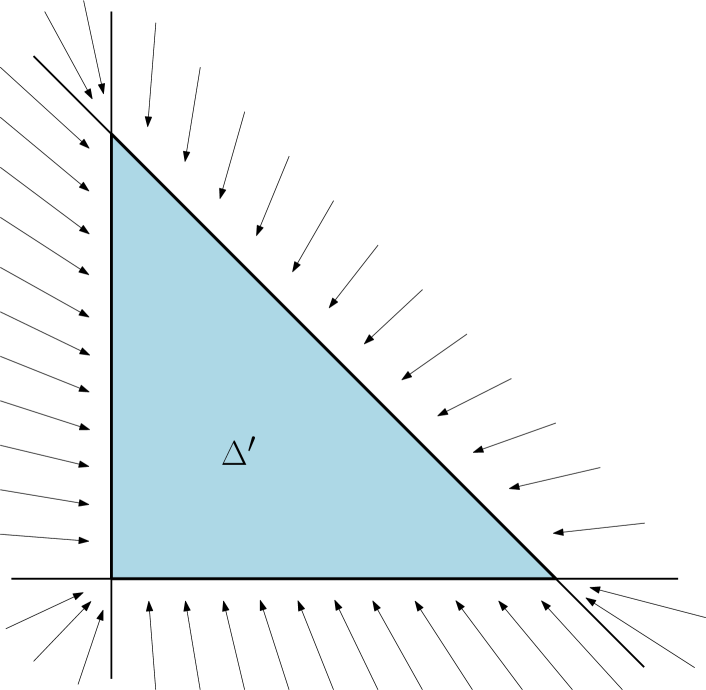
Figure 3: A piece-wise projective approximation to $T$

Denote by $a_{1}^{\prime},a_{2}^{\prime},a_{3}^{\prime}$ the sides of $\Delta^{\prime}$ lying on $l_{1}^{\prime},l_{2}^{\prime},l_{3}^{\prime}$ respectively, and by $v_{1}^{\prime},v_{2}^{\prime},v_{3}^{\prime}$ the opposite vertices. The lines $l_{1}^{\prime},l_{2}^{\prime},l_{3}^{\prime}$ divide the plane into 7 closed domains: $\Delta^{\prime}$, 3 exterior angles $A(v_{i}^{\prime})$ corresponding to the vertices $v_{i}^{\prime}$ and 3 unbounded domains $D(a_{i}^{\prime})$, so that $D(a_{i}^{\prime})$ has the side $a_{i}^{\prime}$ as a part of its boundary.

Pick a vertex $v_{i}^{\prime}$. Introduce polar coordinates $(r,\theta)$ on the plane so that $v_{i}^{\prime}$ is the center of the coordinate system. When a point $x$ runs through the straight line $l_{i}^{\prime}$, the value of $\theta(x)$ runs through an open interval in $S^{1}$ – denote it by $J_{i}\subset S^{1}$. For any $\theta\in J_{i}$ denote by $R_{i}(\theta)$ the distance between $v_{i}^{\prime}$ and the intersection point of $l_{i}^{\prime}$ with the ray from $v_{i}^{\prime}$ having the angle $\theta$ (note that $R_{i}(\theta)\to+\infty$ as $\theta$ approaches an end-point of $J_{i}$). Let $\psi:(0;+\infty)\rightarrow{\mathbb{R}}$ be a smooth function so that $0\leq\psi^{\prime}(t)<K$ for $t\in(0;+\infty)$, $\psi(t)=t$ for $t\in(0;1/2)$, $\psi(t)=1$ for $t\in[1;+\infty)$. In particular, $\psi(t)<Kt$. Define $\phi_{i}:(0;+\infty)\times S^{1}\rightarrow(0;+\infty)$ by

$$\phi_{i}(r,\theta)=\left\{\begin{array}[]{lllll}R_{i}(\theta)\psi(\frac{r}{R_{i}(\theta)}),\text{ if }\theta\in J_{i},\\[3.61371pt] r,\text{ if }\theta\notin J_{i}.\\[3.61371pt] \end{array}\right.$$

An easy check shows that $\phi_{i}$ is a smooth function. We have $\frac{\partial\phi_{i}}{\partial r}(r,\theta)<K$ and $\phi_{i}(r,\theta)<Kr$ for $(r,\theta)\in(0;+\infty)\times S^{1}$. Define $\Phi_{i}:{\mathbb{R}}^{2}\rightarrow{\mathbb{R}}^{2}$ by $\Phi_{i}(r,\theta)=(\phi_{i}(r,\theta),\theta)$ for $(r,\theta)\in(0;+\infty)\times S^{1}$, and $\Phi_{i}(v_{i}^{\prime})=v_{i}^{\prime}$. Then at the point $(r,\theta)$ we have

$$\Phi_{i}^{*}\omega=\frac{\phi_{i}(r,\theta)}{r}\frac{\partial\phi_{i}}{\partial r}(r,\theta)\omega$$

and hence

$$|d\Phi_{i}|=\frac{\phi_{i}(r,\theta)}{r}\frac{\partial\phi_{i}}{\partial r}(r,\theta)<K^{2},$$

since we know that $\frac{\partial\phi_{i}}{\partial r}(r,\theta)<K$ and $\phi_{i}(r,\theta)<Kr$ for $(r,\theta)\in(0;+\infty)\times S^{1}$. The map $\Phi_{i}$ maps the region $D(a_{i}^{\prime})$ onto $a_{i}^{\prime}$. Moreover, it maps the region $A(v_{i+1}^{\prime})$ (we use the cyclic numbering of vertices modulo $3$) onto the ray starting at $v_{i+1}^{\prime}$ and going outwards from $\Delta^{\prime}$ along $l_{i}^{\prime}$. Similarly, $\Phi_{i}$ maps the region $A(v_{i+2}^{\prime})$ onto the ray starting at $v_{i+2}^{\prime}$ and going outwards from $\Delta^{\prime}$ along $l_{i}^{\prime}$.

Consider an affine map $\Psi:{\mathbb{R}}^{2}\rightarrow{\mathbb{R}}^{2}$ defined by

$$\Psi(s,t)=\bigg{(}\frac{s-\delta}{1-\delta},\frac{t-\delta}{1-\delta}\bigg{)}$$

in the standard coordinates $(s,t)$. Then $\|d\Psi\|=K^{2}$. Now define $T:{\mathbb{R}}^{2}\rightarrow{\mathbb{R}}^{2}$ by $T=\Psi\circ\Phi_{1}\circ\Phi_{2}\circ\Phi_{3}$. We have $|dT|\leqslant K^{8}$, and it is easy to see that $T$ maps $\{s\leq\delta\}$ to $\{s=0\}$, $\{t\leq\delta\}$ to $\{t=0\}$, $\{s+t\geq 1-\delta\}$ to $\{s+t=1\}$. Finally it remains to take $K=\sqrt[8]{1+\kappa}$.   ∎

Put

$$pb^{\prime}_{3}:=\inf_{(F^{\prime},G^{\prime})\in{\mathcal{F}}^{\prime}_{3}(X,Y,Z)}||\{F^{\prime},G^{\prime}\}||.$$

Clearly, $pb_{3}\leq pb^{\prime}_{3}$. Thus it is enough to show that $pb_{3}\geq pb^{\prime}_{3}$.

Indeed, let $(F,G)\in{\mathcal{F}}_{3}(X,Y,Z)$, that is

$$F|_{X}\leq 0,G|_{Y}\leq 0,(F+G)|_{Z}\geq 1.$$

Take $T$ from Lemma 2.4 (with a small enough $\kappa>0$) and put

$$F^{\prime}=T_{1}(F,G),G^{\prime}=T_{2}(F,G).$$

An immediate check shows that $(F^{\prime},G^{\prime})\in{\mathcal{F}}^{\prime}_{3}(X,Y,Z)$ and

$$||\{F^{\prime},G^{\prime}\}||\leq||\{F,G\}||(1+\kappa).$$

Choosing $\kappa$ arbitrarily small and taking the infimums over $(F^{\prime},G^{\prime})$ and $(F,G)$ in both sides of the inequality we get that

$$pb^{\prime}_{3}\leq pb_{3},$$

and hence $pb_{3}=pb^{\prime}_{3}$, as required.   ∎

Proof of Proposition 1.3(ii). Set

$$pb_{4}:=pb_{4}(X_{0},X_{1},Y_{0},Y_{1}),$$

$$pb^{\prime}_{4}:=\inf_{(F,G)\in{\mathcal{F}}^{\prime}_{4}(X_{0},X_{1},Y_{0},Y_{1})}||\{F,G\}||.$$

Clearly,

$$pb_{4}\leq pb^{\prime}_{4},$$

so it suffices to prove that

$$pb_{4}\geq pb^{\prime}_{4}.$$ (34)

Fix $\epsilon>0$. Choose $(F,G)\in{\mathcal{F}}_{4}(X_{0},X_{1},Y_{0},Y_{1})$ so that

$$pb_{4}\geq||\{F,G\}||-\epsilon.$$

Fix a small enough $\delta>0$ and choose a smooth non-decreasing function $u:{\mathbb{R}}\to[0;1]$ so that $u(s)=0$ for $s\leq\delta$, $u(s)=1$ for $s\geq 1-\delta$ and $u^{\prime}(s)\leq 1+2\delta$. Put $\phi=u\circ F$ and $\psi=u\circ G$. An immediate check shows that $(\phi,\psi)\in{\mathcal{F}}^{\prime}_{4}(X_{0},X_{1},Y_{0},Y_{1})$. Now note that

$$pb^{\prime}_{4}\leq||\{\phi,\psi\}||\leq$$

$$\leq(1+2\delta)^{2}\cdot||\{F,G\}||\leq(1+2\delta)^{2}(pb_{4}+\epsilon).$$

Choosing $\epsilon$ and $\delta$ arbitrarily small, we get (34) which completes the proof.  ∎

Proof of Proposition 2.3. By monotonicity,

$$pb_{4}(X_{0}\cup A,X_{1},Y_{0},Y_{1})\geq pb_{4}(X_{0},X_{1},Y_{0},Y_{1}).$$

Let us prove the reverse inequality. Fix $\epsilon>0$. By Proposition 1.3(ii), there exist functions $F,G\in C^{\infty}(M)$ with $F=0$ on ${\it Op}(X_{0})$, $F=1$ on ${\it Op}(X_{1})$, $G=0$ on ${\it Op}(Y_{0})$, $G=1$ on ${\it Op}(Y_{1})$, and

$$pb_{4}(X_{0},X_{1},Y_{0},Y_{1})\geq||\{F,G\}||-\epsilon.$$

Let $U\subset{\it Op}(Y_{0})$ be a neighborhood of $A$, $U\cap X_{1}=\emptyset$. Choose a smooth cut-off function $u:M\to[0;1]$ which vanishes on $A$ and equals $1$ outside $U$. Put $F^{\prime}=uF$. Note that

$$\{F^{\prime},G\}=u\{F,G\}+F\{u,G\}.$$

If $x\in U$, the function $G$ is constant near $x$ and hence $\{F^{\prime},G\}=\{F,G\}=0$. If $x\notin U$, we have $u=1$ near $x$ and hence again $\{F^{\prime},G\}=\{F,G\}$. Thus $\{F^{\prime},G\}=\{F,G\}$ everywhere and therefore, since $F^{\prime}=0$ on $X_{0}\cup A$ and $F^{\prime}=1$ on $X_{1}$, we get that

$$pb_{4}(X_{0}\cup A,X_{1},Y_{0},Y_{1})\leq||\{F^{\prime},G\}||=||\{F,G\}||\leq pb_{4}(X_{0},X_{1},Y_{0},Y_{1})+\epsilon.$$

Since this holds for every $\epsilon>0$, we get that

$$pb_{4}(X_{0}\cup A,X_{1},Y_{0},Y_{1})\leq pb_{4}(X_{0},X_{1},Y_{0},Y_{1})$$

which completes the proof.  ∎

3 Symplectic approximation

In this section we prove the results on symplectic approximation stated in Section 1.3.

3.1 The Lipschitz property of the function $s\rho_{F,G}$

Proof of Proposition 1.6: Fix $c>0$. Then for any $\epsilon>0$ there exist $F^{\prime},G^{\prime}$ such that $\|\{F^{\prime},G^{\prime}\}\|\leqslant c$ and $\|F-F^{\prime}\|+\|G-G^{\prime}\|<\rho_{F,G}(c)+\epsilon$. Take any $0<\lambda<1$ and denote $F_{1}=\lambda F^{\prime}$, $G_{1}=G^{\prime}$. Then $(F_{1},G_{1})\in K_{\lambda c}$, and we have

$$\|F-F_{1}\|+\|G-G_{1}\|=\|F-\lambda F^{\prime}\|+\|G-G^{\prime}\|\leqslant$$

$$\leqslant\|F-F^{\prime}\|+(1-\lambda)\|F^{\prime}\|+\|G-G^{\prime}\|\leqslant\rho_{F,G}(c)+\epsilon+(1-\lambda)\|F^{\prime}\|\leqslant$$

$$\leqslant\rho_{F,G}(c)+\epsilon+(1-\lambda)\|F^{\prime}-F\|+(1-\lambda)\|F\|\leqslant$$

$$\leqslant\rho_{F,G}(c)+\epsilon+(1-\lambda)\rho_{F,G}(c)+(1-\lambda)\epsilon+(1-\lambda)\|F\|\leqslant$$

$$\leqslant\rho_{F,G}(c)+\epsilon+(1-\lambda)\|F\|+(1-\lambda)\epsilon+(1-\lambda)\|F\|=$$

$$=\rho_{F,G}(c)+2\|F\|(1-\lambda)+(2-\lambda)\epsilon.$$

Therefore $\rho_{F,G}(\lambda c)\leqslant\rho_{F,G}(c)+2\|F\|(1-\lambda)+(2-\lambda)\epsilon$. This is true for any $\epsilon>0$, hence $\rho_{F,G}(\lambda c)\leqslant\rho_{F,G}(c)+2\|F\|(1-\lambda)$. Therefore

$$|\lambda c\rho_{F,G}(\lambda c)-c\rho_{F,G}(c)|\leqslant|\lambda c\rho_{F,G}(\lambda c)-c\rho_{F,G}(\lambda c)|+|c\rho_{F,G}(\lambda c)-c\rho_{F,G}(c)|=$$

$$=\rho_{F,G}(\lambda c)|\lambda c-c|+c(\rho_{F,G}(\lambda c)-\rho_{F,G}(c))\leqslant$$

$$\leqslant\|F\|(c-\lambda c)+2c\|F\|(1-\lambda)=$$

$$=3\|F\|(c-\lambda c).$$

This is true for any $c>0$, $1>\lambda>0$. Therefore the function $s\mapsto s\rho_{F,G}(s)$ is Lipschitz on $(0;+\infty)$ with the Lipschitz constant $3\|F\|$. Since $\rho_{F,G}=\rho_{G,F}$, the same property is true with the Lipschitz constant $3||G||$ which finishes the proof.   ∎

3.2 The profile function and Poisson bracket invariants

Proof of Theorem 1.4(ii). Assume, without loss of generality, that $0\leq F\leq 1$. Choose $H\in C^{\infty}_{c}(M)$ such that $H=1/2$ on the union of the supports of $F$ and $G$ and $0\leq H\leq 1/2$. Then $\{H,G\}=0$ and

$$\rho_{F,G}(0)\leq d((F,G),(H,G))=||F-H||\leq 1/2.$$

Therefore, as soon as we prove (9) and (10), we would get $\rho_{F,G}(0)=1/2$. Furthermore, for any $t\in[0,1]$ we have $||\{tF+(1-t)H,G\}||=||\{tF,G\}||$ and therefore the pair $(tF+(1-t)H,G)$ lies in ${\mathcal{K}}_{t||\{F,G\}||}$. Thus $\rho_{F,G}(t||\{F,G\}||)\leq d((F,G),(tF+(1-t)H,G))=(1-t)||F-H||\leq 1/2-t/2$. Setting $s:=t||\{F,G\}||$ we get $\rho_{F,G}(s)\leq 1/2-s/(2||\{F,G\}||)$, that is (8).

Thus it remains to prove inequalities (9) and (10).

The case $(F,G)\in{\mathcal{F}}_{3}^{\flat}(X,Y,Z)$:

Fix $s\in[0;p)$. Suppose that $\rho_{F,G}(s)<1/2$ (otherwise (9) follows automatically). Take any $\delta\in(\rho_{F,G}(s),1/2)$. Take $(H,K)\in{\mathcal{F}}=C^{\infty}_{c}(M)\times C^{\infty}_{c}(M)$ with $d((F,G),(H,K))\leq\delta$ and

$$||\{H,K\}||\leq s.$$

Put

$$\alpha:=||F-H||,\beta:=||G-K||.$$

Thus $\alpha+\beta\leq\delta$. Furthermore,

$$H|_{X}\leq\alpha,K|_{Y}\leq\beta,(H+K)|_{Z}\geq 1-\delta.$$

Set

$$H_{1}:=\frac{H-\alpha}{1-2\delta},\ K_{1}:=\frac{K-\beta}{1-2\delta}.$$

Then

$$H_{1}|_{X}\leq 0,\,K_{1}|_{Y}\leq 0,\,(H_{1}+K_{1})|_{Z}\geq 1.$$

Note that, unlike $H$ and $K$, the functions $H_{1},K_{1}$ are not necessarily compactly supported but are constant outside a compact set (if $M$ is not closed). Pick a smooth compactly supported function $u:M\to[0;1]$ so that $u\equiv 1$ on an open neighborhood of $X\cup Y\cup Z\cup{\rm supp}\,H\cup{\rm supp}\,K$. Set $H_{2}:=uH_{1}$, $K_{2}:=uK_{1}$. An easy check shows that

$$||\{H_{2},K_{2}\}||=||\{H_{1},K_{1}\}||.$$

On the other hand, $(H_{2},K_{2})\in{\mathcal{F}}$ and

$$H_{2}|_{X}\leq 0,\,K_{2}|_{Y}\leq 0,\,(H_{2}+K_{2})|_{Z}\geq 1.$$

Therefore, by the definition of $pb_{3}$, we have

$$||\{H_{2},K_{2}\}||\geq p=pb_{3}(X,Y,Z).$$

Note that

$$||\{H_{2},K_{2}\}||=||\{H_{1},K_{1}\}||=\frac{1}{(1-2\delta)^{2}}\cdot||\{H,K\}||\leq\frac{s}{(1-2\delta)^{2}}.$$

Thus

$$\frac{s}{(1-2\delta)^{2}}\geq p$$

and therefore

$$\delta\geq\frac{1}{2}-\frac{1}{2\sqrt{p}}\cdot\sqrt{s}.$$

Since this is true for every $\delta\in(\rho_{F,G}(s),1/2)$ we get that

$$\rho_{F,G}(s)\geq\frac{1}{2}-\frac{1}{2\sqrt{p}}\cdot\sqrt{s},$$

as required.

The case $(F,G)\in{\mathcal{F}}_{4}^{\flat}(X_{0},X_{1},Y_{0},Y_{1})$:

Fix $s\in[0;p)$. Suppose that $\rho_{F,G}(s)<1/2$ (otherwise (10) follows automatically). Take any $\delta\in(\rho_{F,G}(s),1/2)$. Take $(H,K)\in{\mathcal{F}}=C^{\infty}_{c}(M)\times C^{\infty}_{c}(M)$ with $d((F,G),(H,K))\leq\delta$ and

$$||\{H,K\}||\leq s.$$

Put

$$\alpha:=||F-H||,\beta:=||G-K||.$$

Thus $\alpha+\beta\leq\delta$ and, in particular, $0\leq\alpha,\beta\leq\delta<1/2$. Furthermore,

$$H|_{X_{0}}\leq\alpha,H|_{X_{1}}\geq 1-\alpha,K|_{Y_{0}}\leq\beta,K|_{Y_{1}}\geq 1-\beta.$$

Set

$$H_{1}:=\frac{H-\alpha}{1-2\alpha},\ K_{1}:=\frac{K-\beta}{1-2\beta}.$$

Then

$$H_{1}|_{X_{0}}\leq 0,H_{1}|_{X_{1}}\geq 1,K_{1}|_{Y_{0}}\leq 0,K_{1}|_{Y_{1}}\geq 1.$$

Note that, unlike $H$ and $K$, the functions $H_{1},K_{1}$ are not necessarily compactly supported but are constant outside a compact set (if $M$ is not closed). Pick a smooth compactly supported function $u:M\to[0;1]$ so that $u\equiv 1$ on an open neighborhood of $X_{0}\cup X_{1}\cup Y_{0}\cup Y_{1}\cup{\rm supp}\,H\cup{\rm supp}\,K$. Set $H_{2}:=uH_{1}$, $K_{2}:=uK_{1}$. An easy check shows that

$$||\{H_{2},K_{2}\}||=||\{H_{1},K_{1}\}||.$$

On the other hand, $(H_{2},K_{2})\in{\mathcal{F}}$ and

$$H_{2}|_{X_{0}}\leq 0,H_{2}|_{X_{1}}\geq 1,K_{2}|_{Y_{0}}\leq 0,K_{2}|_{Y_{1}}\geq 1.$$

Therefore, by the definition of $pb_{4}$, we have

$$||\{H_{1},K_{1}\}||=||\{H_{2},K_{2}\}||\geq p=pb_{4}(X_{0},X_{1},Y_{0},Y_{1}).$$

Note that

$$||\{H_{1},K_{1}\}||=\frac{1}{(1-2\alpha)(1-2\beta)}\cdot||\{H,K\}||.$$

Since $\alpha,\beta\geq 0$ and $\alpha+\beta\leq\delta$,

$$(1-2\alpha)(1-2\beta)\geq 1-2(\alpha+\beta)+4\alpha\beta\geq 1-2\delta.$$

Thus $s/(1-2\delta)\geq p$ and therefore $\delta\geq 1/2-s/(2p)$. Since this is true for every $\delta\in(\rho_{F,G}(s),1/2)$, we get that $\rho_{F,G}(s)\geq 1/2-s/(2p)$ as required.   ∎

Remark 3.1.

Theorem 1.4(ii) has the following generalization concerning iterated Poisson brackets of two functions.

Namely, denote by ${\mathcal{P}}_{N}$, $N\geq 2$, the set of Lie monomials in two variables of degree $N$ (i.e. if the Lie brackets are denoted by $\{\cdot,\cdot\}$, the set ${\mathcal{P}}_{2}$ consists of $\{A,B\}$, ${\mathcal{P}}_{3}$ of $\{\{A,B\},A\}$ and $\{\{A,B\},B\}$, and so on). For $F,G\in(C^{\infty}_{c}(M),\{\cdot,\cdot\})$ set

$$Q_{N}(F,G):=\sum_{p\in{\mathcal{P}}_{N}}||p(F,G)||,$$

$${\mathcal{K}}_{s}^{(N)}:=\{(F,G)\in{\mathcal{F}}:Q_{N}(F,G)\leq s\}.$$

In particular, for $N=2$ we get the sets ${\mathcal{K}}_{s}$ defined in Section 1.2: ${\mathcal{K}}_{s}={\mathcal{K}}_{s}^{(2)}$. The sets ${\mathcal{K}}_{s}^{(N)}$ can be viewed as “tubular neighborhoods” of the set of Poisson-commuting pairs of functions on $M$: indeed, a symplectic version of the Landau-Hadamard-Kolmogorov inequality (see [17], [18]) implies that ${\mathcal{K}}_{0}^{(N)}={\mathcal{K}}_{0}$ for any $N$. Now, similarly to $\rho_{F,G}$, define a new profile function (cf. [18]):

$$\rho_{F,G}^{(N)}(s):=d((F,G),{\mathcal{K}}_{s}^{(N)}).$$

In particular, for $N=2$ we get the profile function $\rho_{F,G}$ studied above: $\rho_{F,G}^{(2)}=\rho_{F,G}$.

It turns out that, similarly to Theorem 1.4(ii), for certain $(F,G)$ one can estimate $\rho_{F,G}^{(N)}(s)$ from below for small $s$ using an analogue of $pb_{3}$ for iterated Poisson brackets. Namely, given a triple $(X,Y,Z)$ of compact subsets of $M$ with $X\cap Y\cap Z=\emptyset$, define

$$pb_{3}^{(N)}(X,Y,Z):=\inf_{(F,G)}Q_{N}(F,G),$$

where the infimum is taken over ${\mathcal{F}}_{3}(X,Y,Z)$.

Then the proof of Theorem 1.4(ii) can be carried over directly to the case of iterated Poisson brackets yielding the following claim:

Put $p_{N}=pb_{3}^{(N)}(X,Y,Z)$ and let ${\mathcal{F}}_{3}^{\flat}$ be defined as in Section 1.3. Assume that $p_{N}>0$.

Then for every $(F,G)\in{\mathcal{F}}_{3}^{\flat}$ the profile function $\rho_{F,G}^{(N)}$ is continuous. It satisfies $\rho_{F,G}^{(N)}(0)=1/2$ and

$$\rho_{F,G}^{(N)}(s)\geq\frac{1}{2}-\frac{C(N)}{p_{N}^{1/N}}s^{1/N},$$

for all $s\in[0;p)$, where $C(N)>0$ is a positive constant depending only on $N$.

Let us note that a similar result for another class of pairs $(F,G)$ (defined by means of a symplectic quasi-state) has been proved in [18]. It would be interesting to find out whether such a lower bound on the profile function is (asymptotically) exact.

It follows from [18] that $pb_{3}^{(N)}(X,Y,Z)>0$ for all $N\geq 2$ provided the sets $X,Y,Z$ are superheavy (see Section 1.5 above).

One can similarly define the natural analogue $pb_{4}^{(N)}$ of the $pb_{4}$-invariant in the context of iterated Poisson brackets, and repeat the proof of Theorem 1.4(ii) to get a lower bound for the generalized profile function $\rho_{F,G}^{(N)}$. However, at the moment we have no tools for proving the positivity of $pb_{4}^{(N)}$ in any example.

3.3 The two-dimensional case

In the two-dimensional case, the continuity of the profile function at $0$ readily follows from the following result by Zapolsky.

Proposition 3.2 ([49]).

Let $(M,\omega)$ be a closed connected $2$-dimensional symplectic manifold. Let $(F,G)\in{\mathcal{F}}$ be a pair of functions with $\|\{F,G\}\|\leqslant s$. Then there exist a pair of Poisson-commuting functions $(F^{\prime},G^{\prime})\in{\mathcal{F}}$ with $\|F-F^{\prime}\|+\|G-G^{\prime}\|\leqslant C\sqrt{s}$, where the constant $C$ depends only on $(M,\omega)$.

In other words, every almost commuting pair of functions is nearly commuting, that is it can be approximated by a commuting pair. Similar statements for various types of matrices and, more generally, elements of $C^{*}$-algebras have been extensively studied – see e.g. [37, 27] and the references therein. However, no analogue of Proposition 3.2 is known for higher-dimensional symplectic manifolds and there might be a counterexample.

Proof of Proposition 1.9. Fix $\delta>0$ small enough. Take $(F_{1},G_{1})\in{\mathcal{K}}_{s}$ with

$$d((F,G),(F_{1},G_{1}))\leq\rho_{F,G}(s)+\delta.$$

By Proposition 3.2, there exist Poisson-commuting functions $F_{2}$ and $G_{2}$ with

$$d((F_{1},G_{1}),(F_{2},G_{2}))\leq C\sqrt{s}.$$

By the triangle inequality,

$$\rho_{F,G}(0)\leq d((F,G),(F_{2},G_{2}))\leq\rho_{F,G}(s)+C\sqrt{s}+\delta$$

for every $\delta>0$. This yields inequality (12).   ∎

3.4 Sharpness of the convergence rate: an example

Proof of Theorem 1.5:

We need to show that

$$\rho_{F,G}(\varepsilon)\leq\rho_{F,G}(0)-C\sqrt{\varepsilon}$$

for some $C>0$ and any sufficiently small $\varepsilon$ (since $\rho_{F,G}$ is non-increasing, by choosing a smaller $C$ we can get the inequality for any $\epsilon$).

The standard symplectic form on the upper hemi-sphere can be expressed as $\omega=\frac{dx\wedge dy}{\sqrt{1-x^{2}-y^{2}}}$, while on the lower hemi-sphere we have $\omega=-\frac{dx\wedge dy}{\sqrt{1-x^{2}-y^{2}}}$. Therefore, for a given pair of functions $f,g:S^{2}\rightarrow{\mathbb{R}}$, on the upper hemi-sphere we have

$$\{f(x,y),g(x,y)\}_{S^{2}}=\sqrt{1-x^{2}-y^{2}}\{f(x,y),g(x,y)\}_{{\mathbb{R}}^{2}(x,y)},$$

while on the lower hemi-sphere we have

$$\{f(x,y),g(x,y)\}_{S^{2}}=-\sqrt{1-x^{2}-y^{2}}\{f(x,y),g(x,y)\}_{{\mathbb{R}}^{2}(x,y)}.$$

In any case we have

$$|\{f(x,y),g(x,y)\}_{S^{2}}|=\sqrt{1-x^{2}-y^{2}}\ |\{f(x,y),g(x,y)\}_{{\mathbb{R}}^{2}(x,y)}|.$$

Our purpose is to find smooth functions $F_{1},G_{1}:S^{2}\rightarrow{\mathbb{R}}$, depending on a small parameter $\varepsilon>0$, such that $\|F_{1}-F\|+\|G_{1}-G\|\leqslant 1/2-O(\varepsilon)$, while $\|\{F_{1},G_{1}\}\|\leqslant O(\varepsilon^{2})$. We will search for functions $F_{1},G_{1}$ of the form $F_{1}=f(x^{2},y^{2})$, $G_{1}=g(x^{2},y^{2})$, where $f,g:\bigtriangleup=\{(t,s)|t,s\geqslant 0,t+s\leqslant 1\}\rightarrow{\mathbb{R}}$ are smooth functions. Further on we use the notation $t=x^{2}$, $s=y^{2}$. We have

$$\|F_{1}-F\|+\|G_{1}-G\|=\|f(t,s)-t\|_{\bigtriangleup}+\|g(t,s)-s\|_{\bigtriangleup},$$

while

$$|\{F_{1},G_{1}\}_{S^{2}}|=|\{f(x^{2},y^{2}),g(x^{2},y^{2})\}_{S^{2}}|$$

$$=\sqrt{1-x^{4}-y^{4}}\ |\{f(x^{2},y^{2}),g(x^{2},y^{2})\}_{{\mathbb{R}}^{2}(x,y)}|$$

$$=4\sqrt{1-x^{4}-y^{4}}\ |xy||\{f(t,s),g(t,s)\}_{{\mathbb{R}}^{2}(t,s)}|$$

$$=4\sqrt{(1-t^{2}-s^{2})ts}\ |\{f(t,s),g(t,s)\}_{{\mathbb{R}}^{2}(t,s)}|.$$

For our purposes it is enough to find smooth $f,g:\bigtriangleup\rightarrow{\mathbb{R}}$ that satisfy

$$\|f(t,s)-t\|_{\bigtriangleup}+\|g(t,s)-s\|_{\bigtriangleup}\leqslant 1/2-O(\varepsilon),$$

$$\|\{f(t,s),g(t,s)\}_{{\mathbb{R}}^{2}(t,s)}\|\leqslant O(\varepsilon^{2}).$$

Consider new coordinates $u=t-s$, $v=t+s$. In these coordinates we have $\bigtriangleup=\{(u,v)|0\leqslant v\leqslant 1,-v\leqslant u\leqslant v\}$. We take the functions $f,g$ to be of the form

$$f(u,v)=\phi(v)+u\psi(v),$$

$$g(u,v)=\phi(v)-u\psi(v),$$

for some $\phi,\psi:[0,1]\to{\mathbb{R}}$, or, in regular coordinates $(t,s)$,

$$f(t,s)=\phi(t+s)+(t-s)\psi(t+s),$$

$$g(t,s)=\phi(t+s)-(t-s)\psi(t+s).$$

We have

$$\{f,g\}_{{\mathbb{R}}^{2}(t,s)}=2\{f,g\}_{{\mathbb{R}}^{2}(u,v)}=2\{\phi(v)+u\psi(v),\phi(v)-u\psi(v)\}_{{\mathbb{R}}^{2}(u,v)}$$

$$=-4\{\phi(v),u\psi(v)\}_{{\mathbb{R}}^{2}(u,v)}=-4\psi(v)\{\phi(v),u\}_{{\mathbb{R}}^{2}(u,v)}=4\psi(v)\phi^{\prime}(v).$$

First, let us find a pair of continuous functions $\phi,\psi$, such that

$$\|f(t,s)-t\|_{\bigtriangleup},\|g(t,s)-s\|_{\bigtriangleup}\leqslant 1/4-\varepsilon.$$ (35)

The image of the corresponding map $T:(s,t)\mapsto(f(s,t),g(s,t))$ consists of the union of a segment and a triangle attached to it, see Figure 4.

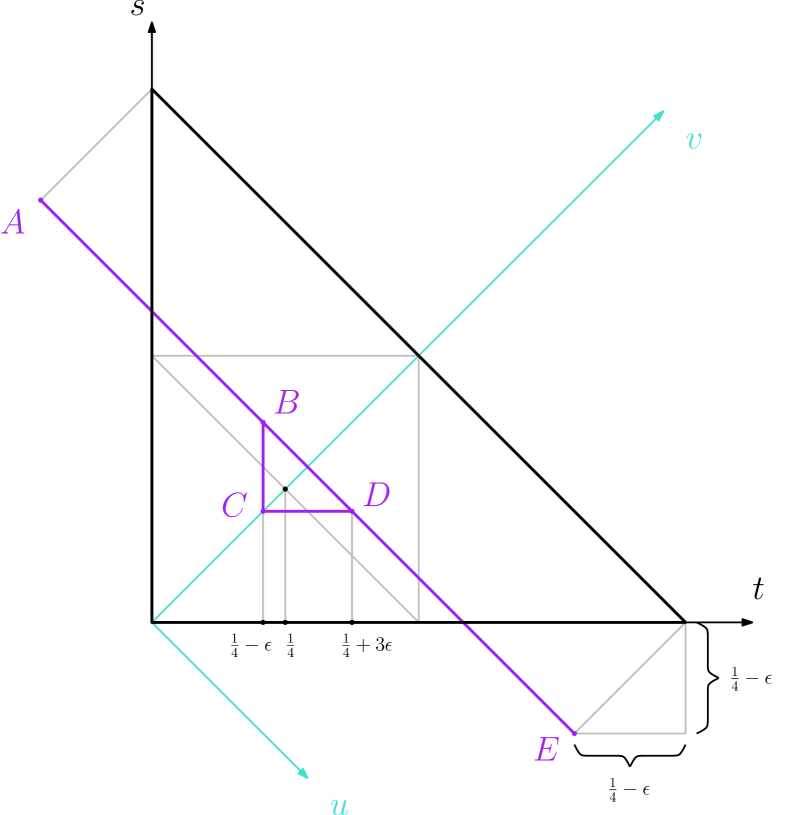
Figure 4: The image of $T$: $[A;E]\cup\triangle BCD$

Because of the symmetry, in order to verify (35) it is enough to check only that $\|f(t,s)-t\|_{\bigtriangleup}\leqslant 1/4-\varepsilon$. We have $f(t,s)-t=f(u,v)-(u+v)/2=\phi(v)+u\psi(v)-u/2-v/2$. For a fixed $v$ this is a linear function of $u$. Recall that $\bigtriangleup=\{(u,v)|0\leqslant v\leqslant 1,-v\leqslant u\leqslant v\}$. As a conclusion, it is enough to check the inequality $|f(u,v)-(u+v)/2|=|\phi(v)+u\psi(v)-u/2-v/2|\leqslant 1/4-\varepsilon$ only for the cases $u=v$ and $u=-v$ while $0\leqslant v\leqslant 1$. Substituting $u=v$, $u=-v$ we see that it is enough to check that

$$|\phi(v)+v\psi(v)-v|\leqslant 1/4-\varepsilon,$$

$$|\phi(v)-v\psi(v)|\leqslant 1/4-\varepsilon$$

for $0\leqslant v\leqslant 1$. We define our continuous $\phi,\psi$ to be

$$\phi(v)=(1/4-\varepsilon)+4\varepsilon v\text{ for }v\in[0;1/2],$$

$$\phi(v)=1/4+\varepsilon\text{ for }v\in[1/2;1],$$

and

$$\psi(v)=4\varepsilon\text{ for }v\in[0;1/2],$$

$$\psi(v)=(1-4\varepsilon)+\frac{1}{v}(-1/2+4\varepsilon)\text{ for }v\in[1/2;1].$$

Because of our choice of the functions $\phi,\psi$, the functions $\phi(v),v\psi(v)$ are linear on each one of intervals $[0;1/2]$ and $[1/2;1]$, and hence the functions $\phi(v)+v\psi(v)-v,\phi(v)-v\psi(v)$ are linear on the intervals $[0;1/2]$ and $[1/2;1]$ as well. Therefore it is enough to check that

$$|\phi(v)+v\psi(v)-v|\leqslant 1/4-\varepsilon$$

and

$$|\phi(v)-v\psi(v)|\leqslant 1/4-\varepsilon$$

only for $v=0,1/2,1$. We have

$$\phi(0)+0\cdot\psi(0)-0=\phi(0)=1/4-\varepsilon,$$

$$\phi(1/2)+1/2\psi(1/2)-1/2=(1/4+\varepsilon)+4\varepsilon/2-1/2=-1/4+3\varepsilon,$$

$$\phi(1)+1\cdot\psi(1)-1=(1/4+\varepsilon)+1/2-1=-1/4+\varepsilon,$$

$$\phi(0)-0\cdot\psi(0)=\phi(0)=1/4-\varepsilon,$$

$$\phi(1/2)-\psi(1/2)/2=(1/4+\varepsilon)-4\varepsilon/2=1/4-\varepsilon,$$

$$\phi(1)-1\cdot\psi(1)=(1/4+\varepsilon)-1/2=-1/4+\varepsilon.$$

In all the cases the absolute value of the result is not bigger than $1/4-\varepsilon$.

Hence we have found continuous $\phi,\psi:[0;1]\rightarrow{\mathbb{R}}$ for which

$$\|f(t,s)-t\|_{\bigtriangleup},\|g(t,s)-s\|_{\bigtriangleup}\leqslant 1/4-\varepsilon.$$

One can easily make the functions $\phi,\psi$ smooth by a sufficiently $C^{0}$-small perturbation so that we will still have $\|f(t,s)-t\|_{\bigtriangleup},\|g(t,s)-s\|_{\bigtriangleup}\leqslant 1/4-\varepsilon/2$, and, moreover,

$$|\phi^{\prime}(v)|\leqslant 4\varepsilon\text{ for }v\in[0;1/2],$$

$$|\phi^{\prime}(v)|\leqslant 32\varepsilon^{2}\text{ for }v\in[1/2;1],$$

$$|\psi(v)|\leqslant 4\varepsilon\text{ for }v\in[0;1/2],$$

$$|\psi(v)|\leqslant 1/2\text{ for }v\in[1/2;1].$$

Then for any $v\in[0;1]$ we have $|4\psi(v)\phi^{\prime}(v)|\leqslant 64\varepsilon^{2}$. As a conclusion, we obtain

$$\|f(t,s)-t\|_{\bigtriangleup}+\|g(t,s)-s\|_{\bigtriangleup}\leqslant(1/4-\varepsilon/2)+(1/4-\varepsilon/2)=1/2-\varepsilon,$$

and

$$|\{f,g\}_{{\mathbb{R}}^{2}(t,s)}|=|4\psi(v)\phi^{\prime}(v)|\leqslant 64\varepsilon^{2}$$

at any point $(t,s)\in\bigtriangleup$.   ∎

Remark 3.3.

At the moment we are unable to decide whether the example constructed above has a counterpart in the context of matrix algebras (for instance, for $su(n)$).

4 Detecting Hamiltonian chords

4.1 Proofs of the results about Hamiltonian chords

In this section we prove Theorems 1.11,1.12 and part (ii) of Corollary 1.17.

Proof of Theorem 1.11. Let $X_{0},X_{1}\subset M$ be disjoint compact subsets, and let $G$ be a function from $C^{\infty}_{c}(M)$. Set

$$Pb(X_{0},X_{1};G):=\inf||\{F,G\}||,$$

where the infimum is taken over all functions $F\in C^{\infty}_{c}(M)$ with $F|_{X_{0}}\leq 0,F|_{X_{1}}\geq 1$, and

$$Pb^{\prime}(X_{0},X_{1};G):=\inf||\{F,G\}||,$$

where the infimum is taken over all functions $F\in C^{\infty}_{c}(M)$ with $F|_{X_{0}}=0,F|_{X_{1}}=1$.

Put $T=T(X_{0},X_{1};G)$ and let $F$ be any smooth compactly supported function with

$$F|_{X_{0}}\leq 0,F|_{X_{1}}\geq 1.$$

There exist $i\in\{0;1\}$ and $x\in X_{i}$ so that $g_{T}x\in X_{1-i}$ (recall that $g_{t}$ is the Hamiltonian flow of $G$). Thus $|F(g_{T}x)-F(x)|\geq 1$, which yields $||\{F,G\}||\geq T^{-1}$. Therefore

$$T(X_{0},X_{1};G)\geq\frac{1}{Pb(X_{0},X_{1};G)}.$$

Since, obviously, $Pb(X_{0},X_{1};G)\leq Pb^{\prime}(X_{0},X_{1};G)$, it remains to prove that

$$T(X_{0},X_{1};G)\leq\frac{1}{Pb^{\prime}(X_{0},X_{1};G)}.$$

We shall need the following lemma.

Lemma 4.1.

Let $v$ be a smooth compactly supported vector field on $M$ and $X_{0},X_{1}$ be a pair of disjoint compact subsets of $M$. Denote by $g_{t}$ the flow of $v$. Assume that $g_{t}X_{0}\cap X_{1}=\emptyset$ for all $t\in[-a;a]$ for some $a>0$. Then there exists a smooth compactly supported function $F:M\to[0;1]$ such that $F|_{X_{0}}=0,F|_{X_{1}}=1$ and $||L_{v}F||<1/a$.

Proof of Lemma 4.1. Choose $b>a$, sufficiently close to $a$, so that $g_{t}X_{0}\cap X_{1}=\emptyset$ for all $t\in[-b;b]$. The sets

$$\check{X}_{0}:=\bigcup_{t\in[0;b]}g_{t}(X_{0})$$

and

$$\check{X}_{1}:=\bigcup_{t\in[0;b]}g_{t}(X_{1})$$

do not intersect. Take any smooth compactly supported function $H:M\to[0;1]$ so that $H=0$ on $\check{X}_{0}$ and $H=1$ on $\check{X}_{1}$. Put

$$F:=\frac{1}{b}\int_{0}^{b}H\circ g_{t}\;dt.$$

Clearly, $F$ has values in $[0;1]$, is compactly supported, $F=0$ on $X_{0}$, $F=1$ on $X_{1}$ and

$$L_{v}F=\frac{1}{b}\int_{0}^{b}\frac{d}{dt}H\circ g_{t}\;dt=\frac{1}{b}(H\circ g_{b}-H).\;$$

It follows that $||L_{v}F||\leq 1/b<1/a$, and we are done.   ∎

Let us return to the proof of the theorem. Put $v=\operatorname{sgrad}G$. Assume on the contrary that

$$T(X_{0},X_{1};G)>\frac{1}{Pb^{\prime}(X_{0},X_{1};G)}.$$

Thus there exists

$$a>\frac{1}{Pb^{\prime}(X_{0},X_{1};G)}$$

so that $g_{t}X_{0}\cap X_{1}=\emptyset$ for all $t\in[-a;a]$. By Lemma 4.1, there exists a smooth compactly supported function $F:M\to[0;1]$ so that $F|_{X_{0}}=0,F|_{X_{1}}=1$ and $||L_{v}F||<1/a$. But $L_{v}F=\{F,G\}$ and we conclude that $Pb^{\prime}(X_{0},X_{1},Y_{0},Y_{1})<1/a$, which means a contradiction. This completes the proof.   ∎

Proof of Theorem 1.12. Choose $a>0$ so that

$$\max G-\min G<R-a.$$ (36)

Let $u:{\mathbb{R}}\to[0;+\infty)$ be a cut-off function which is equal to $1$ on the interval $[-(R-a);R-a]$ and whose support lies in $(-R;R)$. Consider a new autonomous compactly supported Hamiltonian

$$H:M\times{\mathbb{A}}_{R}\to{\mathbb{R}},\;(x,r,\theta)\to u(r)(G(x,\theta)+r)\;$$

generating a Hamiltonian flow $h_{t}$. Since $H\leq 0$ on ${\text{stab}}_{R}Y_{0}$ and $H\geq 1$ on ${\text{stab}}_{R}Y_{1}$, Theorem 1.10 guarantees existence of a point $z=(y,0,\theta_{0})\in{\text{stab}}_{R}X_{0}$ and $T\in[-1/p;1/p]$ so that $h_{T}z\in{\text{stab}}_{R}X_{1}$.

We claim that the piece of trajectory $z(t)=\{h_{t}z\}$, $t\in[0;T]$ is entirely contained in the domain $V=\{|r|<R-a\}\subset M\times{\mathbb{A}}_{R}$. Indeed, assuming the contrary, choose $\tau\in[0;T]$ so that $h_{\tau}z\in\partial V$. Write $z(t)=(x(t),r(t),\theta(t))$. We have that $r(0)=0$ and $r(\tau)=\pm(R-a)$. By the energy conservation law, $H(z(0))=H(z(\tau))$ and hence

$$G(z(0),\theta(0))=G(z(\tau),\theta(\tau))\pm(R-a).$$

This contradicts assumption (36) and the claim follows.

It follows that $u(r(t))=1$ for all $t\in[0;T]$. Hence the projection of $z(t)$ to $M$ is a curve $\alpha$ of the form $\{g_{\theta_{0}+t}g_{\theta_{0}}^{-1}y\}$, $t\in[0;T]$. Put $x=g_{\theta_{0}}^{-1}y$, $t_{0}=\theta_{0}$ and $t_{1}=\theta_{0}+T$. We see that $g_{t_{0}}x=y\in X_{0}$ and $g_{t_{1}}x=x(T)\in X_{1}$. Thus $\alpha$ is a required Hamiltonian chord.   ∎

Proof of Corollary 1.17, part (ii). Choose $R>\max G-\min G$. Identify the annulus $A_{R}$ with the sphere $S^{2}$ of area $2R$ with punctured the North and the South Poles. Under this identification the zero section $\{r=0\}$ corresponds to the equator, say $E$, of the sphere. Thus we consider $M\times{\mathbb{A}}_{R}$ as a domain in $M\times S^{2}$. The latter manifold is equipped with the symplectic form $\omega+2R\sigma$, where $\sigma$ is the standard area form on $S^{2}$ of the total area $1$. The $S^{2}$-stability of the quasi-state $\zeta$ on $(M,\omega)$ yields a quasi-state ${\widetilde{\zeta}}_{2R}$ on $(M\times S^{2},\omega+2R\sigma)$. Denote by $K_{2R}$ the constant from the PB-inequality for ${\widetilde{\zeta}}_{2R}$.

Assume that the sets $X_{0}\cup Y_{0},Y_{0}\cup X_{1},X_{1}\cup Y_{1},Y_{1}\cup X_{0}$ are superheavy. Due to the $S^{2}$-stability of $\zeta$, the sets

$$(X_{0}\cup Y_{0})\times E,(Y_{0}\cup X_{1})\times E,(X_{1}\cup Y_{1})\times E,(Y_{1}\cup X_{0})\times E$$

are all superheavy with respect to the quasi-state ${\widetilde{\zeta}}_{2R}$. By inequality (28) and Theorem 1.15,

$$pb_{4}({\text{stab}}_{R}X_{0},{\text{stab}}_{R}X_{1},{\text{stab}}_{R}Y_{0},{\text{stab}}_{R}Y_{1})\\ \geq pb_{4}(X_{0}\times E,X_{1}\times E,Y_{0}\times E,Y_{1}\times E)\geq\frac{1}{4K_{2R}}.$$

Finally, the existence of the required Hamiltonian chord follows now from Theorem 1.12. This finishes the proof.   ∎

Remark 4.2.

Note that if we assume that $Y_{1}$ is superheavy (and so are $X_{0}\cup Y_{0}$ and $X_{1}\cup Y_{0}$), then the constant appearing in the previous proof can be improved from ${1}/({4K_{2R}})$ to ${1}/{K_{2R}}$. Indeed, by the $S^{2}$-stability of the quasi-state on $(M,\omega)$, the sets $(X_{0}\cup Y_{0})\times E,(X_{1}\cup Y_{0})\times E,Y_{1}\times E$ are superheavy with respect to ${\widetilde{\zeta}}_{2R}$. Then, by (17),

$$pb_{4}({\text{stab}}_{R}X_{0},{\text{stab}}_{R}X_{1},{\text{stab}}_{R}Y_{0},{\text{stab}}_{R}Y_{1})\geq\frac{1}{K_{2R}}.$$

4.2 Miscellaneous remarks

Let us make a few more remarks on the interplay between superheaviness and Hamiltonian chords for autonomous Hamiltonians. In this section we assume that $M$ is closed.

Remark 4.3 (Recurrence of Hamiltonian chords).

Let $F$ be a smooth function on $M$. Denote its Hamiltonian flow by $f_{t}$. Put $Y_{0}=\{F\leq 0\}$ and $Y_{1}=\{F\geq 1\}$. A subset $X$ is called a ballast if $X\cup Y_{i}$ is superheavy for $i=0,1$. For instance, in Example 1.18 above the role of ballasts is played by the Lagrangian discs $C^{v}$.

Given two ballasts $X_{0},X_{1}$, denote by $P\subset{\mathbb{R}}$ the set of all $\tau$ such that $f_{\tau}X_{0}\cap X_{1}\neq\emptyset$. We claim that Hamiltonian chords between $X_{0}$ and $X_{1}$ exhibit a recurrent behavior in the following sense: The set $P$ intersects every interval of time-length $8K$. Indeed, since $Y_{i}$ are invariant under $f_{t}$, the image of a ballast under $f_{t}$ is again a ballast. Take any $s\notin P$ so that $f_{s}X_{0}\cap X_{1}=\emptyset$. Thus the quadruple $(f_{s}X_{0},X_{1},Y_{0},Y_{1})$ satisfies the assumptions of Corollary 1.17. Hence there exists $t\in[-4K;4K]$ so that $f_{t+s}X_{0}=f_{t}f_{s}X_{0}$ intersects $X_{1}$, and the claim follows.

Remark 4.4 (Energy control).

Let us follow the notations and the set-up of the previous example. Fix an interval $I=[a;b]$ with $0\leq a<b\leq 1$ and put $X_{i}^{I}=X_{i}\cap F^{-1}(I)$, $i=0,1$, where $X_{i}$, $i=0,1$, are disjoint ballasts.

We claim there exists a Hamiltonian chord of $f_{t}$ of time-length $8K/(b-a)$ which touches both $X_{0}^{I}$ and $X_{1}^{I}$.

Interestingly enough, this statement has a flavor of time-energy uncertainty: we have to pay for the precision of our knowledge of the energy level carrying a chord by an uncertainty in our knowledge of the time interval on which the chord is defined.

To prove the claim put $Y_{0}^{\prime}=\{F\leq a\},Y_{1}^{\prime}=\{F\geq b\}$. One can deduce from Proposition 2.3 that

$$pb_{4}(X_{0}^{I},X_{1}^{I},Y_{0}^{\prime},Y_{1}^{\prime})=pb_{4}(X_{0},X_{1},Y_{0}^{\prime},Y_{1}^{\prime})\geq\frac{1}{4K}.$$

Put $F^{\prime}=(F-a)/(b-a)$. Then $F^{\prime}\leq 0$ on $Y_{0}^{\prime}$ and $F^{\prime}\geq 1$ on $Y_{1}^{\prime}$. Therefore, by Theorem 1.10, the Hamiltonian flow $f^{\prime}_{t}$ of $F^{\prime}$ admits a chord of time-length at most $8K$ touching both $X_{0}^{I}$ and $X_{1}^{I}$. The claim follows from the fact that $f_{t}=f^{\prime}_{t(b-a)}$.

Remark 4.5 (Producing rigid subsets from flexible ones).

Let $X_{0}$, $Y_{0}$, $Y_{1}$ be subsets of $M$ so that $Y_{0}$ and $Y_{1}$ are disjoint, and $X_{0}\cup Y_{0},Y_{1}\cup X_{0}$ are superheavy. Take any Hamiltonian $G$ such that $G|_{Y_{0}}\leq 0,G|_{Y_{1}}\geq 1$ and denote by $g_{t}$ its Hamiltonian flow. Put

$$Z:=\bigcup_{t\in[-4K;4K]}g_{t}X_{0}.$$

Theorem 1.15 implies that $Z$ intersects every superheavy subset $X_{1}\subset M$ and hence exhibits a “symplectically rigid” behavior. To illustrate this, assume in addition that the quasi-state $\zeta$ is invariant under the identity component $Symp_{0}$ of the symplectomorphism group of $(M,\omega)$: this happens in all known higher-dimensional examples. Let $r_{0}(M,\omega):=\sup r(B)$, where $r(B)$ is the radius of a symplectically embedded open ball $B\subset M$ and the supremum is taken over all balls $B$ whose complement contains a superheavy subset. It follows that $Z$ cannot be mapped into any symplectically embedded ball $B\subset M$ of radius $r<r_{0}(M,\omega)$ by a diffeomorphism from ${\hbox{\it Symp}}_{0}$. A somewhat paradoxical point here is that $X_{0}$ itself could be absolutely “flexible”, e.g. a closed Lagrangian disc. Of course, the Hamiltonian function $G$ as above is quite special, hence there is no contradiction.

Example 4.6.

Here we present a construction of subsets $X_{0},X_{1},Y_{0},Y_{1}$ satisfying the assumptions of Theorem 1.15 (ii). Let $A_{i}$, $i=1,2,3,4$, be four closed superheavy subsets such that no three of them have a common point. Put $A_{ij}:=A_{i}\cap A_{j}$. Present each $A_{i}$ as a union of closed subsets, $A_{i}=B_{i}\cup C_{i}$, so that

$$B_{i}\cap C_{i}\cap A_{ij}=\emptyset\;\forall i,j,$$

and

• $A_{12}\cup A_{13}\subset B_{1}$, $A_{14}\subset C_{1}$;

• $A_{23}\cup A_{24}\subset B_{2}$, $A_{21}\subset C_{2}$;

• $A_{34}\subset B_{3}$, $A_{31}\cup A_{32}\subset C_{3}$;

• $A_{41}\subset B_{4}$, $A_{42}\cup A_{43}\subset C_{4}$.

Put

$$X_{0}:=B_{1}\cup C_{2},Y_{0}:=B_{2}\cup C_{3},X_{1}:=B_{3}\cup C_{4},Y_{1}:=B_{4}\cup C_{1}.$$

Obviously, the sets $X_{0}\cup Y_{0}$, $Y_{0}\cup X_{1}$, $X_{1}\cup Y_{1}$, $Y_{1}\cup X_{0}$ contain superheavy sets $A_{2}$, $A_{3}$, $A_{4}$, $A_{1}$ respectively. At the same time it is straightforward to check that

$$X_{0}\cap X_{1}=Y_{0}\cap Y_{1}=\emptyset,$$

as required.

One can also construct a quadruple of sets satisfying the assumptions of Theorem 1.15 from a triple of superheavy sets. Namely, assume $A,B,C\subset M$ are closed superheavy sets with $A\cap B\cap C=\emptyset$. Let $U$ be an open neighborhood of $A\cap B$ such that $\overline{U}$ is disjoint from $C$. Set $X_{0}:=\overline{U}\cap(A\cup B)$, $X_{1}:=C$, $Y_{0}:=A\setminus U$, $Y_{1}:=B\setminus U$. Then $X_{0},X_{1},Y_{0},Y_{1}$ satisfy the assumptions of Theorem 1.15. By Proposition 2.3, formula (32) and monotonicity, $pb_{4}(X_{0},X_{1},Y_{0},Y_{1})\geq pb_{3}(A,B,C)$. Note that if $A,B,C$ are, for instance, superheavy Lagrangian submanifolds intersecting transversally and $U$ is the complement of a sufficiently small closed tubular neighborhood of $C$, the sets $Y_{0}$ and $Y_{1}$ given by this construction are finite unions of small Lagrangian discs.

Remark 4.7.

Let us compare the bounds on the time-length of Hamiltonian chords given by Theorem 1.10 (the autonomous case) and Theorem 1.12 (the non-autonomous case). We will compare the bounds for the case of an autonomous Hamiltonian and for $R=+\infty$ (i.e. when both estimates are applicable and there are no restrictions on the oscillation of the Hamiltonian). We have seen in (30) above that

$$1/pb_{4}(X_{0},X_{1},Y_{0},Y_{1})\leq 1/pb_{4}({\text{stab}}X_{0},{\text{stab}}X_{1},{\text{stab}}Y_{0},{\text{stab}}Y_{1}).$$ (37)

Thus for Hamiltonian chords of autonomous Hamiltonians the “autonomous” bound from Theorem 1.10 is a priori better than the “non-autonomous” one from Theorem 1.12. As it was mentioned above, the “autonomous” bound is sharp and therefore whenever one has the equality in (37) the “non-autonomous” bound is sharp as well (see Theorem 1.20 and Proposition 1.21 above for an example where the equality in (37) is actually reached). It would be interesting to find out whether the bound on the time-length of the Hamiltonian chord given by Theorem 1.12 is always sharp. In other words, the question is whether for any compact $X_{0},X_{1},Y_{0},Y_{1}\subset M$, $X_{0}\cap X_{1}=Y_{0}\cap Y_{1}=\emptyset$, one can find time-dependent Hamiltonians as in Theorem 1.12 admitting Hamiltonian chords that connect $X_{0}$ and $X_{1}$ and have time-lengths arbitrarily close to $1/pb_{4}({\text{stab}}X_{0},{\text{stab}}X_{1},{\text{stab}}Y_{0},{\text{stab}}Y_{1})$.

5 Poisson brackets and pseudo-holomorphic polygons

5.1 Defining polygons

Let ${\mathbb{D}}\subset{\mathbb{C}}$ be the unit disc. Take $k\geq 2$ pairwise distinct points $z_{0},\ldots,z_{k-1}$ on the unit circle in $\partial{\mathbb{D}}$ in the counter-clockwise cyclic order (thus further on we use the convention $(k-1)+1=0$ for the indices). They divide the circle into $k$ arcs

$$a_{0}=[z_{k-1};z_{0}],a_{1}=[z_{0};z_{1}],\ldots,a_{k-1}=[z_{k-2};z_{k-1}].$$

Let ${\mathcal{L}}=(L_{0},\ldots,L_{k-1})$ be a collection of Lagrangian submanifolds in a symplectic manifold $(M,\omega)$. A parameterized $k$-gon with boundary on ${\mathcal{L}}$ is a smooth map $\phi:{\mathbb{D}}\to M$ such that $\phi(a_{i})\subset L_{i}$ for all $i$. For the sake of brevity we shall often refer to the image $\phi({\mathbb{D}})$ as to a $k$-gon with boundary on ${\mathcal{L}}$ with edges $\phi(a_{i})$ and (cyclically oriented) vertices $\phi(z_{i})$. The $k$-gons are called triangles for $k=3$ and quadrilaterals for $k=4$.

Denote by ${\mathbb{D}}(z_{0},\ldots,z_{k-1})$ the unit disc in ${\mathbb{C}}$ with $k$ counter-clockwise cyclically ordered marked points $z_{0},\ldots,z_{k-1}$ on the boundary. The space ${\mathcal{P}}^{k}$ of all such discs is naturally identified with a subset of $(\partial{\mathbb{D}})^{k}$. The group $PU(1,1)$ acts on ${\mathcal{D}}$ by holomorphic automorphisms, and hence acts on ${\mathcal{P}}^{k}$. Given an almost complex structure $J$ on $(M,\omega)$ consider the set of all pairs $(z,\phi)$ where $z=(z_{0},\ldots,z_{k-1})\in{\mathcal{P}}^{k}$ and $\phi:{\mathbb{D}}(z_{0},\ldots,z_{k-1})\to M$ is a $J$-holomorphic parameterized $k$-gon with boundary on ${\mathcal{L}}$. Its quotient by the natural action of the group $PU(1,1)$ is called the moduli space of $J$-holomorphic $k$-gons with boundary on ${\mathcal{L}}$ and is denoted by ${\mathcal{M}}$ (with some extra decorations which will be introduced later).

5.2 A reminder on the Maslov class

Let $\ell_{1},\ell_{2}$ be a pair of Lagrangian subspaces in a symplectic vector space $V$. Pick any compatible almost complex structure $J$ on $V$ with $J\ell_{1}=\ell_{2}$. Denote by $\gamma_{J}(L_{1},L_{2})$ the path $e^{tJ}\ell_{1}$, $t\in[0;\pi/2]$, of Lagrangian subspaces joining $\ell_{1}$ with $\ell_{2}$.

Let now $L_{0},\ldots,L_{k-1}$ be a collection of Lagrangian submanifolds of a symplectic manifold $(M^{2n},\omega)$ in general position: every pair from this collection intersects transversally and there are no triple intersections. Let $P$ be a $k$-gon whose edges $e_{i}$ lie on $L_{i}$. Choose a parametrization $e_{i}(t)$ of the edges yielding the cyclic orientation of the boundary of the polygon. Denote by $v_{i,i+1}$ the vertex lying on $L_{i}\cap L_{i+1}$, where the indices are taken modulo $k$.

Let $\Lambda M\to M$ be a canonical fibration whose fiber over a point $x\in M$ is the Lagrangian Grassmannian $\Lambda_{n}(T_{x}M)$. For every edge $e_{i}$ consider its canonical lift $\hat{e}_{i}(t)=T_{e_{i}(t)}L_{i}$ to $\Lambda M$. Fix an $\omega$-compatible almost complex structure $J$ on $M$. The curves

$$\hat{e}_{0},\gamma_{J}(T_{v_{0,1}}L_{0},T_{v_{0,1}}L_{1}),\hat{e}_{1},\gamma_{J}(T_{v_{1,2}}L_{1},T_{v_{1,2}}L_{2}),\ldots,$$

$$\ldots\hat{e}_{k-1},\gamma_{J}(T_{v_{k-1,0}}L_{k-1},T_{v_{k-1,0}}L_{0})$$

form a loop, say $\theta$, in $\Lambda M$.

Take a symplectic trivialization of the tangent bundle $TM$ over $P$ so that the restriction of $\Lambda M$ to $P$ splits as $P\times\Lambda_{n}$, where $\Lambda_{n}$ is the Lagrangian Grassmannian (the space of Lagrangian planes in the symplectic vector space ${\mathbb{R}}^{2n}$). Write $\theta^{\prime}$ for the projection of $\theta$ to $\Lambda_{n}$.

Recall that ${\mathcal{T}}_{k}$ is the set of homotopy classes of $k$-gons in $M$ whose sides (in the natural cyclic order) lie, respectively, in $L_{0},L_{1},\ldots,L_{k-1}$. Let $\alpha=[P]\in{\mathcal{T}}_{k}$ be the homotopy class of a $k$-gon $P$. By definition, the Maslov index $m(\alpha)$ is the Maslov index of $\theta^{\prime}$ in $\Lambda_{n}$. This definition is independent of the choices of $J$, the specific polygon $P$ inside the homotopy class $\alpha$ and the symplectic trivialization. We refer to [23, 47] for the details.

5.3 Gluing polygons

Let ${\mathcal{L}}=(L_{0},\ldots,L_{k-1})$ be a collection of Lagrangian submanifolds of a symplectic manifold $(M^{2n},\omega)$ in general position. Given a homotopy class $\alpha$ of polygons with boundary on ${\mathcal{L}}$, we can perform two operations on it:

• Take a representative $P$ of $\alpha$ and attach a disc with the boundary on some $L_{i}$ at a point lying on the $i$-th edge of $P$;

• Attach a sphere at a point of $P$.

We say that two homotopy classes $\alpha$ and $\beta$ of the polygons are equivalent if $\beta$ can be obtained from $\alpha$ by a sequence of such operations. For brevity we shall write

$$\beta=\alpha+\sum_{i=0}^{k-1}D_{i}+S,$$

where $D_{i}\in\pi_{2}(M,L_{i})$ and $S\in\pi_{2}(M)$. Observe that this representation is not unique: for instance, $S\in\pi_{2}(M,L_{i})$ for all $i$. The Maslov indices of $\alpha$ and $\beta$ are related by the standard formula (cf. [47])

$$m(\beta)=m(\alpha)+\sum m_{L_{i}}(D_{i})+2c_{1}(S),$$ (38)

where $m_{L_{i}}$ is the Maslov class of $L_{1}$ and $c_{1}$ is the first Chern class of $(M,\omega)$.

We shall need also another gluing operation. Let $P$ be a $k$-gon with vertices $p_{j}\in L_{j}\cap L_{j+1}$, $j=0,\ldots,k-1$, with boundary on ${\mathcal{L}}$ and let $\alpha$ be a digon with vertices $v,p_{i}$ and boundaries on $(L_{i},L_{i+1})$ (the marked points $z_{0},z_{1}\in\partial{\mathbb{D}}$ are mapped, respectively, to $v$ and $p_{i}$; accordingly, the arcs $a_{0},a_{1}\subset\partial D$ are mapped, respectively, into $L_{i+1}$ and $L_{i}$). Attaching $\alpha$ to $P$ along $p_{i}$ we get in a natural way a new $k$-gon $P^{\prime}$ with boundary on ${\mathcal{L}}$ and the vertices

$$p_{0},\ldots,p_{i-1},v,p_{i+1},\ldots,p_{k-1}.$$

We shall write $P^{\prime}=\alpha\;\sharp\;P$. The homotopy class of $P^{\prime}$ in ${\mathcal{T}}_{k}$ does not depend on the specific choice of $P$ and $\alpha$ within their homotopy classes. It will be denoted by $[\alpha]\;\sharp\;[P]$. It is easy to check that

$$m([\alpha]\;\sharp\;P)=m([P])+m([\alpha])-n.$$ (39)

Proposition 5.1.

Let $(L,K)$ be a finite type collection of Lagrangian submanifolds. Let $\alpha$ be a digon with boundaries on $(L,K)$ with the same vertices: $\alpha\in{\mathcal{T}}_{2}(a,a)$. Suppose that $m(\alpha)=n$. Then $\omega(\alpha)=0$.

Proof. Changing, if necessary, the orientation of $\alpha$ we can assume that $\omega(\alpha)=c\geq 0$. Put $\alpha_{d}:=\alpha\;\sharp\;\ldots\;\sharp\;\alpha$ taken $d$ times. Then, by (39), we have that $m(\alpha_{d})=n$ while $\omega(\alpha_{d})=dc$. Thus, by the finite type condition, $dc$ is bounded as $d\to\infty$, and hence $c=0$.   ∎

5.4 Finite type collections of Lagrangian submanifolds

Here we discuss examples of finite type collections of Lagrangian submanifolds.

Proof of Proposition 1.26. Let ${\mathcal{L}}=(L_{0},\ldots,L_{k-1})$ be a collection of monotone Lagrangian submanifolds in general position with the same monotonicity constant. Assume that for every $i$ the morphism $\pi_{1}(L_{i})\to\pi_{1}(M)$ has a finite image. We have to show that the collection ${\mathcal{L}}$ is of finite type. The latter assumption guarantees that there exists only finite number of equivalence classes (in the sense of Section 5.3 above) of homotopy classes of polygons with boundary on ${\mathcal{L}}$. Suppose that $P\sim Q$ and $m(P)=m(Q)$. Since all $L_{i}$ have the same monotonicity constant, formula (38) readily yields $\omega(P)=\omega(Q)$. This, in turn, implies that ${\mathcal{L}}$ is of finite type.   ∎

Consider now the cotangent bundle $T^{*}X$ of a closed manifold $X^{l}$ equipped with the standard symplectic form $\sigma$. Let ${\mathcal{K}}=(K_{0},\ldots,K_{k-1})$ be a collection of Lagrangian sections of $T^{*}X$ of the form $K_{i}=\text{graph}\,dF_{i}$, where $F_{i}$ is a smooth function on $X$. Suppose that ${\mathcal{K}}$ is in general position – in particular, all functions $F_{i+1}-F_{i}$ are Morse. Each intersection point $p\in K_{i}\cap K_{i+1}$ is a critical point of $F_{i+1}-F_{i}$. Denote by $\nu(p)$ its Morse index. One can readily check that for every polygon $P$ with vertices $p_{0},\ldots,p_{k-1}$ and boundary in ${\mathcal{K}}$ one has

$$m(P)=\sum_{i}\nu(p_{i}),\ \sigma(P)=\sum_{i}(F_{i}(p_{i})-F_{i+1}(p_{i})).$$

In particular,

$$0\leq m(P)\leq kl,\;\;\;|\sigma(P)|\leq C({\mathcal{K}}):=2k\cdot\max_{i}||F_{i}||\;$$ (40)

for every polygon $P$ with boundaries on ${\mathcal{K}}$. This is a considerable strengthening of the finite type property for the collection ${\mathcal{K}}$. In particular, it immediately yields the following proposition.

Proposition 5.2.

Let $(L_{0},\ldots,L_{k-1})$ be any finite type collection of Lagrangian submanifolds in a symplectic manifold $(M,\omega)$. Let $K_{i}\subset T^{*}X$, $i=0,\ldots,k-1$ be sections as above. Then the collection $(L_{i}\times K_{i})_{i=0,\ldots,{k-1}}$ in $(M\times T^{*}X,\omega\oplus\sigma)$ is of finite type with

$$A(L_{0}\times K_{0},\ldots,L_{k-1}\times K_{k-1};N)\leq\\ \leq\max\{A(L_{0},\ldots,L_{k};j):j\in[N-kl;N]\}+C({\mathcal{K}}).$$ (41)

Proof. Put $\Omega=\omega\oplus\sigma$. Given a $k$-gon $P$ with boundary on $M\times T^{*}X$ and $m(P)=N$, look at its projections $P_{1}$ and $P_{2}$ to $M$ and to $T^{*}X$ respectively. Then $m(P)=m(P_{1})+m(P_{2})$ and $\Omega(P)=\omega(P_{1})+\sigma(P_{2})$. By (40),

$$-kl\leq m(P_{1})-N\leq 0,\ |\omega(P_{1})-\Omega(P)|\leq C({\mathcal{K}}).$$

Thus

$$|\Omega(P)|\leq\max_{j}A(L_{0},\ldots,L_{k};j)+C({\mathcal{K}}),$$

where $j$ runs over $[N-kl;N]$. Therefore the collection $(L_{i}\times K_{i})$ is of finite type and (41) holds.   ∎

5.5 Preliminaries on Lagrangian Floer homology

Here we sketch a definition of operations in Lagrangian Floer homology (over ${\mathbb{Z}}_{2}$) – the reader is referred to [11], [42], [23] for more details.

Let $(M^{2n},\omega)$ be a spherically monotone symplectic manifold with a “nice” behavior at infinity (e.g. geometrically bounded [4]). Let ${\mathcal{L}}=(L_{0},\ldots,L_{k-1})$ be a collection of $k$ closed connected monotone Lagrangian submanifolds, $k=2,3,4$. Our convention is that the indices of $L_{i}$’s are taken modulo $k$, that is $L_{k}=L_{0}$, etc. Recall that the minimal Maslov number $N_{L}$ of a Lagrangian submanifold is the minimal positive generator of the image of $\pi_{2}(M,L)$ under the Maslov class. We put $N_{L}=+\infty$ if $\pi_{2}(M,L)=0$.

Throughout this section we shall assume that the following conditions hold:

• The whole collection ${\mathcal{L}}$ is of finite type.

• Every pair $(L_{i},L_{i+1})$ forms a collection of finite type.

• The minimal Maslov number $N_{L_{i}}$ of each $L_{i}$ is $\geq 2$.

• In case $N_{L_{i}}=2$, the number of pseudo-holomorphic discs of the Maslov index $2$ passing through a generic point of $L_{i}$ is even. In the terminology of [23] this means that the obstruction class (over ${\mathbb{Z}}_{2}$) of each $L_{i}$ vanishes.

In addition we assume that $L_{i}$’s are in general position, meaning that they intersect pairwise transversally and there are no triple intersections, and if $k=4$, then

$$L_{0}\cap L_{2}=L_{1}\cap L_{3}=\emptyset.$$ (42)

Consider the vector space $CF(L_{i},L_{i+1}):=\text{Span}_{{\mathbb{Z}}_{2}}(L_{i}\cap L_{i+1})$. Fix an $\omega$-compatible almost complex structure $J$ on $M$. Given points $p_{i}\in L_{i-1}\cap L_{i}$, $i=1,\ldots,k$, and a homotopy class $A\in{\mathcal{T}}_{k}$ of $k$-gons with boundary on ${\mathcal{L}}$ and the vertices $p_{1},\ldots,p_{k}$, consider the moduli space ${\mathcal{M}}_{A}(p_{1},\ldots,p_{k})$ of $J$-holomorphic $k$-gons representing class $A$. A standard transversality argument yields that for a generic $J$ this space is a smooth manifold of the dimension

$$\dim{\mathcal{M}}_{A}(p_{1},\ldots,p_{k})=m(A)+n(1-k)+k-3.$$ (43)

Remark 5.3.

To make the transversality argument actually work one needs to deal with a more involved version of the $\bar{\partial}$-equation (see [42]). We shall ignore this point in our sketch. Furthermore, under certain assumptions there is a way to associate an index, say $I(p)$, to each intersection point from $L_{i}\cap L_{i+1}$ after equipping the Lagrangian submanifolds (and hence the intersection points) with an additional structure of a Lagrangian brane. In this case the dimension of the moduli space ${\mathcal{M}}_{A}(p_{1},\ldots,p_{k})$ is given by a more standard expression

$$I(p_{k})-\sum_{i=1}^{k-1}I(p_{i})+k-3\;$$

(see e.g. [42], formula (12.8) ). One can verify that it coincides with (43). We shall not enter the issue of grading.

We shall write $|Y|$ for the cardinality – modulo 2 – of a finite set $Y$. Define a ${\mathbb{Z}}_{2}$-multi-linear map

$$\mu^{k-1}:CF(L_{0},L_{1})\otimes\ldots\otimes CF(L_{k-2},L_{k-1})\to CF(L_{0},L_{k-1})$$

by

$$\mu^{k-1}(p_{1},\ldots,p_{k-1})=\sum_{A}\big{|}{\mathcal{M}}_{A}(p_{1},\ldots,p_{k})\big{|}\cdot p_{k},$$ (44)

where the sum is taken over all $0$-dimensional moduli spaces. Note that the moduli spaces ${\mathcal{M}}_{A}(p_{1},\ldots,p_{k})$ are zero-dimensional (or empty) whenever $m(A)=n(k-1)-k+3$. Since our collection is of finite type, the symplectic areas of all polygons from such moduli spaces are bounded away from infinity. Thus a compactness argument yields that the $0$-dimensional moduli spaces are necessarily finite sets and that the sum in the right-hand side of (44) is finite.

The operation $\mu^{1}:CF(L_{0},L_{1})\to CF(L_{0},L_{1})$ is a differential: $\mu^{1}\circ\mu^{1}=0$: this is guaranteed by Floer gluing/compactness theorems and by the vanishing of the obstruction class. For convenience we denote $\mu^{1}$ by $d$. The corresponding homology $\text{Ker}\,d/\text{Im}\,d$ is called the Lagrangian Floer homology $HF(L_{0},L_{1})$ of $L_{0}$ and $L_{1}$. It is a ${\mathbb{Z}}_{2}$-module. In the same way we define Floer homology $HF(L_{i},L_{j})$ for all $i,j$, and for the sake of brevity use the same notation $d$ for the Floer differentials for all $i,j$. Note that when $k=4$, the intersection condition (42) guarantees that $HF(L_{0},L_{2})=HF(L_{1},L_{3})=0$.

Consider the operation

$$\mu^{2}:CF(L_{0},L_{1})\otimes CF(L_{1},L_{2})\to CF(L_{0},L_{2}).$$

We shall abbreviate $\mu^{2}(a_{1},a_{2})=a_{1}a_{2}$. This operation satisfies the Leibnitz rule

$$d(a_{1}a_{2})=a_{1}\cdot da_{2}+da_{1}\cdot a_{2}$$

and hence descends to an operation in homology:

$$HF(L_{0},L_{1})\otimes HF(L_{1},L_{2})\to HF(L_{0},L_{2}).$$

The latter is called the triangle (or Donaldson) product in Lagrangian Floer homology. If $k=4$, we define the triangle product for the triple $L_{1},L_{2},L_{3}$ in the same way and keep for it the same notation. Note that for $k=4$ the intersection condition (42) guarantees that for pairwise distinct $i,j,l$ the triangle product

$$CF(L_{i},L_{j})\otimes CF(L_{j},L_{l})\to CF(L_{i},L_{l})$$

vanishes already on the chain level. The operation

$$\mu^{3}:CF(L_{0},L_{1})\otimes CF(L_{1},L_{2})\otimes CF(L_{2},L_{3})\to CF(L_{0},L_{2})$$

satisfies the $A_{\infty}$-relation

$$d\mu_{3}(a_{1},a_{2},a_{3})=\mu^{3}(da_{1},a_{2},a_{3})+\mu^{3}(a_{1},da_{2},a_{3})+\mu^{3}(a_{1},a_{2},da_{3})\\ +a_{1}(a_{2}a_{3})+(a_{1}a_{2})a_{3}.$$ (45)

This formula yields two useful facts. First, assume that $\mu^{3}=0$. Then the triangle product is associative: $a_{1}(a_{2}a_{3})=(a_{1}a_{2})a_{3}$. Second, we have the following proposition:

Proposition 5.4.

Assume that $L_{0}\cap L_{2}=L_{1}\cap L_{3}=\emptyset$. Then $\mu^{3}$ descends to an operation in Lagrangian Floer homology

$$HF(L_{0},L_{1})\otimes HF(L_{1},L_{2})\otimes HF(L_{2},L_{3})\to HF(L_{0},L_{2}).$$

By a slight abuse of notation, we shall still denote the homological operation by $\mu^{3}$.

Proof. The assumption on intersections yields that the product $\mu^{2}$ vanishes for every triple $L_{i},L_{i+1},L_{i+2}$. Thus the terms $a_{1}(a_{2}a_{3})$ and $(a_{1}a_{2})a_{3}$ in (45) vanish, which immediately yields the statement of the proposition.   ∎

It is a folkloric fact that the Lagrangian Floer homology and the operations introduced above remain invariant under exact Lagrangian isotopies of the submanifolds $L_{i}$ (of course, in case of the $\mu^{3}$-operation on homology one needs the intersection assumption $L_{0}\cap L_{2}=L_{1}\cap L_{3}=\emptyset$ to remain valid during the isotopies). We are going to discuss a particular case of this statement in a slightly different language: instead of deforming Lagrangian submanifolds we shall deform the symplectic form on $M$. A crucial feature of this setting which significantly simplifies the analysis is that the intersection points from $L_{i}\cap L_{i+1}$ remain fixed and transversal in the process of the deformation.

Consider a deformation $\omega_{s}$, $s\in[0;1]$, $\omega_{0}=\omega$, of the symplectic form $\omega$ through symplectic forms on $M$ which satisfy the following conditions:

• $\omega_{s}=\omega$ near each $L_{i}$ for all $s$;

• $\omega_{s}$ is cohomologous to $\omega$ for all $s$;

• for any $s\in[0;1]$ and any $i=0,\ldots,k-1$ the integrals of the forms $\omega_{s}$ and $\omega$ over discs define the same functional $\pi_{2}(M,L_{i}\cup L_{i+1})\to{\mathbb{R}}$.

Note that $L_{i}$ is a monotone Lagrangian submanifold of $(M,\omega_{s})$ and its monotonicity constant does not depend on $s$. Furthermore, assumptions (F2)-(F4) hold automatically for all $s$. We shall assume in addition that

• the collection ${\mathcal{L}}$ is of finite type with respect to $\omega_{s}$ for all $s\in[0;1]$.

Choose a generic $1$-parametric family $J_{s}$, $s\in[0;1]$, of $\omega_{s}$-compatible almost complex structures. Note that the vector spaces $CF(L_{i},L_{i+1})$ do not depend on $s$. Write $d_{s}$ for the Floer differential on $CF(L_{i},L_{j})$ with $i\neq j$. Denote by $HF_{s}(L_{i},L_{j})$ the Lagrangian Floer homology, and by $\mu^{k-1}_{s}$ the operations associated to the collection ${\mathcal{L}}$. We shall write ${\mathcal{M}}^{s}$ for the moduli space of $J_{s}$-holomorphic polygons with boundaries on ${\mathcal{L}}$ and ${\mathcal{M}}_{B}^{s}(p_{1},\ldots,p_{k})\subset{\mathcal{M}}^{s}$ for the space of ${\mathcal{J}}_{s}$-holomorphic polygons in a homotopy class $B$ with the vertices $p_{1},\ldots,p_{k}$.

Proposition 5.5.

Let $k=3$ or $4$. There exist isomorphisms

$$\phi_{i}:HF_{0}(L_{i},L_{i+1})\to HF_{1}(L_{i},L_{i+1}),\;\;i=0,\ldots,k-2,$$

and $\bar{\phi}_{k-1}:HF_{0}(L_{0},L_{k-1})\to HF_{1}(L_{0},L_{k-1})$ which send $\mu^{k-1}_{0}$ to $\mu^{k-1}_{1}$, i.e.

$$\mu^{k-1}_{1}(\phi_{0}(x_{0}),\ldots,\phi_{k-2}(x_{k-2}))=\bar{\phi}_{k-1}(\mu^{k-1}_{0}(x_{0},\ldots,x_{k-2}))$$ (46)

for all $x_{i}\in HF_{0}(L_{i},L_{i+1}),\;i=0,\ldots,k-2$.

Proof. Note that the differential $d_{s}$ and the operations $\mu^{k-1}_{s}$ can change in the process of deformation only due to bubbling-off. Since $L_{i}$’s are monotone with the minimal Maslov number $\geq 2$, for a generic 1-parametric family $J_{s}$ there is no bubbling-off of $J_{s}$-holomorphic discs and spheres (and we assume that our 1-parametric family is chosen to have this property). By the Gromov-Floer compactness result, other possible degenerations of $J_{s}$-holomorphic polygons can be analyzed by looking at possible degenerations of the disc ${\mathbb{D}}$ with the marked points on the boundary into tree-like connected cusp-curves with the marked points on them. Such an analysis, together with the intersection assumptions $L_{0}\cap L_{1}\cap L_{2}=\emptyset$ for $k=3$ and (42) for $k=4$, shows that the only possible pattern of the bubbling-off is as follows: a $J_{s}$-holomorphic digon $\beta$ with boundaries on some pair $(L_{i},L_{j})$ of index $m(\beta)=n+1$ splits into the sum of two digons $\beta=\beta^{\prime}\;\sharp\;\alpha$ where $m(\alpha)=n$. This splitting can take place for a finite set $T=\{0<t_{1}<\ldots<t_{N}<1\}$ of the parameter $s$ which we will call the critical values. Thus on the intervals

$$[0;t_{1}),\ldots,(t_{l-1};t_{l}),\ldots,(t_{N};1]$$

the Floer homology and the operations do not change and their realizations for different values of the parameter (within such an interval) will be identified. Without loss of generality, we can assume that for every critical parameter $t\in T$ there is a unique digon $\alpha$ with $m(\alpha)=n$. We shall call $\alpha$ an exceptional digon.

Fix a pair $(L,K)$ of distinct Lagrangian submanifolds from our collection. Suppose that for $t\in T$ there exists an exceptional digon $\alpha\in{\mathcal{M}}^{t}_{A}(a,b)$, where $a,b\in L\cap K$. Note that $\omega_{t}(\alpha)>0$ and hence Proposition 5.1 above yields that $a\neq b$. Following Floer [21, Lemma 3.5], define an endomorphism $\psi^{t}$ of $CF(L,K)$ by

$$\psi^{t}(x)=x+(x,a)b,$$ (47)

where $(x,a)$ is the coefficient at $a$ in the expansion of $x$ with respect to the basis $L\cap K$ of $CF(L,K)$. Observe that $\psi^{t}\circ\psi^{t}$ is the identity map (recall that we work over ${\mathbb{Z}}_{2}$) and hence $\psi^{t}$ is an isomorphism. By using a gluing/compactness argument Floer showed in [21] that for a sufficiently small $\epsilon>0$

$$\psi^{t}\circ d_{t-\epsilon}=d_{t+\epsilon}\circ\psi^{t}.$$

Thus $\psi^{t}$ induces an isomorphism

$$\phi^{t}:HF_{t-\epsilon}(L,K)\to HF_{t+\epsilon}(L,K).$$

Taking the composition of isomorphisms $\phi^{t}$ over all critical parameters $t\in T$ we get an isomorphism

$$\phi(L,K):HF_{0}(L,K)\to HF_{1}(L,K).$$ (48)

We claim that these isomorphisms send $\mu^{k-1}_{0}$ to $\mu^{k-1}_{1}$. The proof is based on the very same Floer’s argument. Let us elaborate it in the case $k=4$ (the case $k=3$ is analogous).

Let us study what happens with the operation $\mu^{3}_{s}$ when the parameter $s$ passes a critical value $t\in T$. Let $\alpha\in{\mathcal{M}}^{t}(a,b)$ be the exceptional digon, and $A$ be its homotopy class. We denote by ${\mathcal{M}}^{+}$ and ${\mathcal{M}}^{-}$ the moduli spaces of $J_{s}$-holomorphic $k$-gons for $s\in(t;t+\epsilon)$ and $s\in(t-\epsilon;t)$ respectively, and by $\mu^{3}_{\pm}$ the corresponding $\mu^{3}$-operations.

Case 1: $a,b\in L_{0}\cap L_{1}$. Consider a 0-dimensional moduli space of the form ${\mathcal{M}}^{s}_{B}(b,p_{2},p_{3})$, where $s\in(t-\epsilon,t+\epsilon)$, $p_{2}\in L_{1}\cap L_{2}$, $p_{3}\in L_{2}\cap L_{3}$. It does not change when $s$ passes through the critical value $t$. Take a $J_{t}$-holomorphic quadrilateral $P\in{\mathcal{M}}^{t}_{B}(b,p_{2},p_{3},q)$, $q\in L_{0}\cap L_{3}$, and look at the quadrilateral $\alpha\;\sharp\;P$. A parametric version of the standard compactness/gluing argument for pseudo-holomorphic polygons yields that the following bifurcation takes place: there exists a unique family of pseudo-holomorphic polygons from ${\mathcal{M}}^{s}_{A\;\sharp\;B}(a,p_{2},p_{3},q)$, where either $s\in(t-\epsilon;t)$ or $s\in(t;t+\epsilon)$ but not both, which bubbles off to $\alpha\;\sharp\;P$ as $s=t$ and which disappears as $s$ enters the other half of the interval $(t-\epsilon;t+\epsilon)$. In other words, each $P$ contributes $\pm 1$ to the difference

$$\big{|}{\mathcal{M}}^{+}_{A\;\sharp\;B}(a,p_{2},p_{3},q)\big{|}-\big{|}{\mathcal{M}}^{-}_{A\;\sharp\;B}(a,p_{2},p_{3},q)\big{|}.$$

It follows that

$$(\mu^{3}_{+}(a,p_{2},p_{3}),q)-(\mu^{3}_{-}(a,p_{2},p_{3}),q)=(\mu^{3}_{+}(b,p_{2},p_{3}),q),$$

(recall that we are counting modulo $2$), and hence

$$\mu^{3}_{+}(a,p_{2},p_{3})+\mu^{3}_{+}(b,p_{2},p_{3})=\mu^{3}_{-}(a,p_{2},p_{3}).$$ (49)

The cases when $a,b$ lie in $L_{1}\cap L_{2}$ (respectively, in $L_{2}\cap L_{3}$) yield similar equalities. The only difference with (49) is that the points $a,b$ appear at the second (respectively, at the third) position in $\mu^{3}_{\pm}$.

Case 2: $a,b\in L_{0}\cap L_{3}$. Similarly, we look at the broken quadrilateral $P\;\sharp\;\alpha$, where $P$ lies in the $0$-dimensional moduli space ${\mathcal{M}}^{t}_{B}(p_{1},p_{2},p_{3},a)$, and conclude that $P$ contributes $\pm 1$ to the difference

$$\big{|}{\mathcal{M}}^{+}_{B\;\sharp\;A}(p_{1},p_{2},p_{3},b)\big{|}-\big{|}{\mathcal{M}}^{-}_{B\;\sharp\;A}(p_{1},p_{2},p_{3},b)\big{|}.$$

This yields (modulo $2$)

$$(\mu^{3}_{+}(p_{1},p_{2},p_{3}),b)-(\mu^{3}_{-}(p_{1},p_{2},p_{3}),b)=(\mu^{3}_{-}(p_{1},p_{2},p_{3}),a).$$

For every $q\neq b$

$$(\mu^{3}_{+}(p_{1},p_{2},p_{3}),q)=(\mu^{3}_{-}(p_{1},p_{2},p_{3}),q)\;,$$

and hence (modulo 2)

$$\mu^{3}_{+}(p_{1},p_{2},p_{3})=\mu^{3}_{-}(p_{1},p_{2},p_{3})+(\mu^{3}_{-}(p_{1},p_{2},p_{3}),a)b.$$ (50)

Suppose that the exceptional digon $\alpha$ is associated to the pair $(L_{u},L_{v})$, where $(u,v)=(0,1),(1,2),(2,3)$ or $(0,3)$. Define an isomorphism $\psi^{t}_{ij}$ of $CF(L_{i},L_{j})$ by formula (47) if $(i,j)=(u,v)$ and as the identity map otherwise. Using formulas (47),(49) and (50) we conclude that

$$\mu^{3}_{+}(\psi^{t}_{01}(x_{0}),\psi^{t}_{12}(x_{1}),\psi^{t}_{23}(x_{2}))=\psi^{t}_{03}(\mu^{3}_{-}(x_{0},x_{1},x_{2}))$$ (51)

for all

$$x_{0}\in L_{0}\cap L_{1},x_{1}\in L_{1}\cap L_{2},x_{2}\in L_{2}\cap L_{3}.$$

The composition of $\psi^{t}_{ij}$’s over all $t\in T$ is exactly the isomorphism $\phi(L_{i},L_{j})$ introduced in (48) above. Put

$$\phi(L_{0},L_{1}):=\phi_{0},\;\phi(L_{1},L_{2}):=\phi_{1},\;\phi(L_{2},L_{3}):=\phi_{2},\;\phi(L_{0},L_{3})=\bar{\phi}_{3}.$$

With this notation formula (51) readily yields (46). This completes the proof of the proposition.   ∎

5.6 The product formula

Let ${\mathcal{L}}=(L_{0},\ldots,L_{k-1})$ be a generic collection of Lagrangian submanifolds of a symplectic manifold $(M,\omega)$ satisfying assumptions (F1)-(F4) of Section 5.5 above and the intersection condition (42). Choose a generic collection of $k$ sections ${\mathcal{K}}=(K_{0},\ldots,K_{k-1})$ of $T^{*}S^{1}$. Assume that all $K_{i}$ are exact, that is of the form $K_{i}=\text{graph}\,dF_{i}$ for some functions $F_{i}:S^{1}\to{\mathbb{R}}$. Consider a collection $\widehat{{\mathcal{L}}}:=(\widehat{L}_{i}:=L_{i}\times K_{i})$. It also satisfies properties (F1) -(F4) and (42). Indeed, (F1) and (F2) follow from Proposition 5.2 and the remaining properties readily follow from the definitions.

The Künneth formula in Floer homology (which can be obtained by considering the Floer complexes for a split almost complex structure on $M\times T^{*}S^{1}$) yields

$$HF(\widehat{L}_{i},\widehat{L}_{j})=HF(L_{i},L_{j})\otimes HF(K_{i},K_{j}).$$

With this identification we have that

$$(a\otimes A)\cdot(b\otimes B)=(ab)\otimes(AB)$$ (52)

and

$$\mu^{3}(a\otimes A,b\otimes B,c\otimes C)=\mu^{3}(a,b,c)\otimes(ABC).$$ (53)

It is well-known [22] that the ${\mathbb{Z}}_{2}$-module $HF(K_{i},K_{j})$ is canonically identified with $H^{1}(S^{1},{\mathbb{Z}}_{2})$ so that the product $\mu^{2}$ for ${\mathcal{K}}$ corresponds to the cup-product and the $\mu^{3}$-operation for ${\mathcal{K}}$ vanishes. Let us mention that the product $\mu^{2}$ for ${\mathcal{K}}$ is associative and hence the expression $ABC$ is well-defined.

The conclusion of this discussion is that the operations $\mu^{2}$ and $\mu^{3}$ for $\widehat{{\mathcal{L}}}$ do not vanish, provided they do not vanish for ${\mathcal{L}}$.

The proof of (52) is straightforward and will be omitted. The proof of (53) is a bit more delicate and will be sketched below. For more information on the product formulae see [3].

Sketch of the proof of formula (53): Consider the space ${\mathcal{P}}^{4}$ of all discs with four counterclockwise cyclically ordered boundary points, and denote by $\widetilde{{\mathcal{P}}}^{4}$ its quotient by the natural action of $PU(1,1)$. We shall denote by $\widetilde{P}\in\widetilde{{\mathcal{P}}}^{4}$ the image of $P\in{\mathcal{P}}^{4}$ in $\widetilde{{\mathcal{P}}}^{4}$.

Step 1: Fix the standard complex structure $I$ on $T^{*}S^{1}$. Fix a generic almost complex structure $J$ on $M$. We are studying $J\oplus I$-holomorphic maps $u$ from $P\in{\mathcal{P}}$ to $M\times T^{*}S^{1}$ with boundary on $\widehat{{\mathcal{L}}}$. (In this sketch we will not discuss the regularity of these almost complex structures.)

Each such map has the form $u=(\phi,\psi)$, where $\phi:P\to M$ and $\psi:P\to T^{*}S^{1}$. Using the dimension formula (43) and the fact that the Maslov class is additive with respect to direct sums, we get that the $0$-dimensional moduli space of such maps can arise from two sources:

• The map $\phi$ lies in the $0$-dimensional moduli space of $J$-holomorphic quadrilaterals with boundary on ${\mathcal{L}}$. This picks a finite subset, say $Z$, of possible classes $\widetilde{P}$ in the space $\widetilde{{\mathcal{P}}}^{4}$. To get a generic existence of an $I$-holomorphic map $\psi:P\to T^{*}S^{1}$ with boundary on ${\mathcal{K}}$ so that $[P]\in Z$, the map $\psi$ must lie in a $1$-dimensional component of the moduli space of $I$-holomorphic quadrilaterals with boundary on ${\mathcal{K}}$ – in this case by varying $\psi$ we can “tune in” its source to be in $Z$.

• The same, but with $\phi$ lying in the $1$-dimensional moduli space and $\psi$ lying in the $0$-dimensional moduli space.

Note that the count of $0$-dimensional moduli spaces of pseudo-holomorphic quadrilaterals yields the $\mu^{3}$-operation. Since the latter vanishes for ${\mathcal{K}}$, the scenario (ii) can be disregarded. Thus we shall focus on (i) and study $1$-dimensional components of the moduli space of $I$-holomorphic quadrilaterals with boundary on ${\mathcal{K}}$.

Step 2: Pass to the universal cover ${\mathbb{R}}^{2}:={\mathbb{C}}\to T^{*}S^{1}$ and lift the sections $K_{i}$ (we keep the same notation for the lifts). Look at the holomorphic quadrilaterals formed by $K_{0},K_{1},K_{2},K_{3}$. The holomorphic quadrilaterals of expected dimension $1$ correspond to embedded quadrilaterals with boundary on ${\mathcal{K}}$ which have a unique interior angle $>\pi$. Fix such a quadrilateral and, to make further analysis more transparent, draw it as a non-convex Euclidean quadrilateral $ABCD$ in ${\mathbb{R}}^{2}$, where the vertices are written in the counter-clockwise order and the angle at $C$ is $>\pi$. Introduce also the points $E$, which is the intersection of the edge $AD$ with the ray $[BC)$, and $F$, which is the intersection of the edge $AB$ with the ray $[DC)$, see Figure 5.

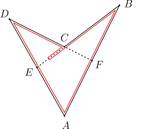
Figure 5: Non-convex quadrilateral $ABCD$

Suppose that

$$AB\subset K_{1},\;BE\subset K_{2},\;FD\subset K_{3},\;DA\subset K_{0}.$$

Introduce a parameter $t\in[0;1]$ on the broken line $ECF$ so that $E$ corresponds to $t=0$, $C$ corresponds to $t=1/2$, $F$ corresponds to $t=1$. Denote by $X_{t}$ the point on the broken line $ECF$ corresponding to the value $t$ of the parameter. Look at the following family of closed broken lines which depends on a parameter $t\in(0,1)$:

• the line formed by the segments $AB\subset K_{1}$, $BX_{t}\subset K_{2}$, $X_{t}C\subset K_{2}$, $CD\subset K_{3}$, $DA\subset K_{0}$ for $t\in(0;1/2)$;

• the line formed by the segments $AB\subset K_{1}$, $BC\subset K_{2}$, $CD\subset K_{3}$, $DA\subset K_{0}$ for $t=1/2$;

• the line formed by the segments $AB\subset K_{1}$, $BC\subset K_{2}$, $CX_{t}\subset K_{3}$, $X_{t}D\subset K_{3}$, $DA\subset K_{0}$ for $t\in(1/2;1)$.

For every $t\in(0;1)$ this broken line bounds a holomorphic polygon, say $\psi_{t}:P_{t}\to{\mathbb{C}}$, where $P_{t}={\mathbb{D}}(z_{0},z_{1},z_{2},z_{3})$, so that

$$\psi_{t}(z_{0})=A,\;\psi_{t}(z_{1})=B,\;\psi_{t}(z_{2})=C,\;\psi_{t}(z_{3})=D.$$

Note that for $t\neq 1/2$ the map $\psi_{t}|_{S^{1}}$ hits $C$ twice, so $z_{2}$ corresponds to the second hit for $t<1/2$ and to the first hit for $t>1/2$. By applying a Möbius transformation we can assume that $z_{0}=-i,z_{1}=1,z_{3}=-1$ and $z_{2}$ varies with $t\in(0;1)$ between $1$ and $-1$ (excluding the endpoints themselves) in the upper half-circle.

Next, we wish to analyze the behavior of these holomorphic quadrilaterals when $t\searrow 0$ and $t\nearrow 1$. For this purpose let us recall (see [22]) that the Deligne-Mumford compactification of $\widetilde{{\mathcal{P}}}^{4}$ can be identified with $[0;1]$, where the boundary point $0$ corresponds to the stable curve

$$\Sigma_{0}:={\mathbb{D}}^{-}(z_{0},z_{1},z_{*})\;\sharp\;{\mathbb{D}}^{+}(z_{*},z_{2},z_{3})$$

and the boundary point $1$ corresponds to the stable curve

$$\Sigma_{1}:={\mathbb{D}}^{-}(z_{0},z_{*},z_{3})\;\sharp\;{\mathbb{D}}^{+}(z_{*},z_{1},z_{2}).$$

Here we denote by ${\mathbb{D}}^{\pm}$ two copies of the unit disc.

When $t\searrow 0$, the bubbling-off happens: The map $\psi_{t}$ converges to a map $\psi_{0}=\psi_{0}^{-}\;\sharp\;\psi_{0}^{+}$ from $\Sigma_{0}$ to ${\mathbb{C}}$. Here $\psi_{0}^{-}:{\mathbb{D}}^{-}\to{\mathbb{C}}$ is a holomorphic triangle with the three sides, respectively, on $K_{0},K_{1},K_{2}$ and the vertices

$$\psi_{0}^{-}(z_{0})=A,\psi_{0}^{-}(z_{1})=B,\psi_{0}^{-}(z_{*})=E,$$

and $\psi_{0}^{+}:{\mathbb{D}}^{+}\to{\mathbb{C}}$ is a holomorphic triangle with the three sides, respectively, on $K_{0},K_{2},K_{3}$ and the vertices

$$\psi_{0}^{+}(z_{*})=E,\psi_{0}^{+}(z_{2})=C,\psi_{0}^{+}(z_{3})=D.$$

Similarly, when $t\nearrow 1$, the map $\psi_{t}$ converges to a map $\psi_{1}=\psi_{1}^{-}\;\sharp\;\psi_{1}^{+}$ from $\Sigma_{1}$ to ${\mathbb{C}}$. Here $\psi_{1}^{-}:{\mathbb{D}}^{-}\to{\mathbb{C}}$ is a holomorphic triangle with the three sides, respectively, on $K_{0},K_{1},K_{3}$ and the vertices

$$\psi_{1}^{-}(z_{0})=A,\psi_{1}^{-}(z_{*})=F,\psi_{1}^{-}(z_{3})=D,$$

and $\psi_{1}^{+}:{\mathbb{D}}^{+}\to{\mathbb{C}}$ is a holomorphic triangle with the three sides, respectively, on $K_{1},K_{2},K_{3}$ and the vertices

$$\psi_{1}^{+}(z_{*})=F,\psi_{1}^{+}(z_{1})=B,\psi_{1}^{+}(z_{2})=C.$$

The bubbling pattern shows that $z_{2}\to z_{3}=-1$ as $t\to 0$ and $z_{2}\to z_{1}=1$ as $t\to 1$. This shows that the map

$$\Phi:[0;1]\to\text{Compactification}(\widetilde{{\mathcal{P}}}^{4}),\;t\to\widetilde{P}_{t},$$

has degree $1$ (modulo 2). Thus, generically, for every $\widetilde{P}\in Z$ (where the finite set $Z$ was defined in Step 1) there exists an odd number of values of $t$ with $\widetilde{P}_{t}=\widetilde{P}$.

Step 3: We use the notations of Steps 1 and 2. Consider all pairs $(P\in{\mathcal{P}}^{4},\phi:P\to M)$ such that the image of $\phi$ is a polygon with vertices $a,b,c,d$. The moduli space of such pairs consists of $(\mu^{3}(a,b,c),d)$ points. We have seen that each such point and every quadrilateral $ABCD\subset T^{*}S^{1}$ as above together contribute $1$ (modulo $2$) to the coefficient

$$(\mu^{3}(a\otimes A,b\otimes B,c\otimes C),d\otimes D).$$

The analysis in Step 2 shows that the number of such quadrilaterals $ABCD$ equals $(A\cdot B\cdot C,D)$. We conclude that

$$(\mu^{3}(a\otimes A,b\otimes B,c\otimes C),d\otimes D)=(\mu^{3}(a,b,c),d)\cdot(A\cdot B\cdot C,D),$$

which immediately yields formula (53).   ∎

We refer to [31] and references therein for an algebraic discussion on $A_{\infty}$-operations for a tensor product of $A_{\infty}$-algebras.

5.7 Application to Poisson brackets invariants

The next result is a more precise version of Theorems 1.27 and 1.30 stated in the introduction. Let ${\mathcal{L}}=(L_{0},\ldots,L_{k-1})$, $k=3$ or $4$, be a collection of Lagrangian submanifolds of a geometrically bounded symplectic manifold. Assume that $L_{i}$’s are in general position, satisfy conditions (F1)-(F4) and for $k=4$ satisfy the intersection condition (42). Put

$$A_{3}=A(L_{0},L_{1},L_{2};2n),A_{4}=A(L_{0},L_{1},L_{2},L_{3};3n-1),$$

$$A^{\prime}_{3}=\max\{A(L_{0},L_{1},L_{2};j):j\in[2n-3;2n]\},$$

$$A^{\prime}_{4}=\max\{A(L_{0},L_{1},L_{2},L_{3};j):j\in[3n-5;3n-1]\}.$$

Theorem 5.6.

Assume that the operation $\mu^{k-1}$ in the Lagrangian Floer homology of ${\mathcal{L}}$ does not vanish. Then

• If $k=3$, then

  $$pb_{3}(L_{0},L_{1},L_{2})\geq\frac{1}{2A_{3}}$$ (54)

  and

  $$pb_{3}({\text{stab}}\,L_{0},{\text{stab}}\,L_{1},{\text{stab}}\,L_{2})\geq\frac{1}{2A^{\prime}_{3}}.$$ (55)

• If $k=4$, then

  $$pb_{4}(L_{0},L_{2},L_{1},L_{3})\geq 1/A_{4}$$ (56)

  and

  $$pb_{4}({\text{stab}}\,L_{0},{\text{stab}}\,L_{2},{\text{stab}}\,L_{1},{\text{stab}}\,L_{3})\geq 1/A^{\prime}_{4}.$$ (57)

Proof. We shall prove part (ii) (the proof of (i) is analogous). By Proposition 1.3, $pb_{4}(L_{0},L_{2},L_{1},L_{3})=\inf{||\{F,G\}||}$, where $F=0$ in a neighborhood of $L_{0}$, $F=1$ in a neighborhood of $L_{2}$, $G=0$ in a neighborhood of $L_{1}$, $G=1$ in a neighborhood of $L_{3}$. Given such functions $F,G\in C^{\infty}_{c}(M)$, consider the family of forms

$$\omega_{s}:=\omega-sdF\wedge dG.$$

Note that

$$dF\wedge dG\wedge\omega^{n-1}=\frac{1}{n}\{F,G\}\cdot\omega^{n}.$$

Thus

$$\omega_{s}^{n}=(1-s\{F,G\})\omega^{n}.$$

Therefore the form $\omega_{s}$ is symplectic for all

$$s\in I:=[0;1/||\{F,G\}||).$$

A straightforward application of the Stokes formula shows that the deformation $\omega_{s}$, $s\in I$, satisfies the assumptions (D1)-(D4) of Section 5.5 above. For instance, in order to verify that the collection ${\mathcal{L}}$ is of finite type for every $s$, observe that $\int_{\alpha}dF\wedge dG=1$ for every quadrilateral $\alpha$ with the boundary on ${\mathcal{L}}$ and hence

$$\omega_{s}(\alpha)\leq\omega(\alpha)-s.$$ (58)

At the same time the Maslov class $m(\alpha)$ does not change in the process of deformation and hence the finite type condition for $\omega_{s}$ follows from the one for $\omega$.

Choose a generic family of almost complex structures $J_{s}$ compatible with $\omega_{s}$. By Proposition 5.5, the operation $\mu^{3}$ in the Lagrangian Floer homology of ${\mathcal{L}}$ with respect to $\omega_{s}$ does not vanish. Thus for every $s\in I$ there exists a $J_{s}$-holomorphic quadrilateral, say $\alpha$, with boundary on ${\mathcal{L}}$. The dimension of the moduli space of such quadrilaterals equals $m(\alpha)-3n+1=0$ and thus the finite type condition (25) guarantees that $\omega(\alpha)\leq A_{4}$. Thus, by (58), $\omega_{s}(\alpha)\leq A_{4}-s$. At the same time $\omega_{s}(\alpha)>0$ and hence $s\leq A_{4}$ for every $s\in I=[0;1/||\{F,G\}||)$. This yields $||\{F,G\}||\geq 1/A_{4}$, and inequality (56) follows.

Let us pass to inequality (57). Choose a collection ${\mathcal{K}}=(K_{0},K_{1},K_{2},K_{3})$ of four generic sections of $T^{*}S^{1}$ and take $\epsilon>0$. Applying Proposition 5.2 and using the product formula (53) we get that the collection $(L_{i}\times\epsilon K_{i})_{i=0,1,2,3}$ also satisfies the assumptions of the theorem and hence, by (56),

$$pb_{4}(L_{0}\times\epsilon K_{0},L_{2}\times\epsilon K_{2},L_{1}\times\epsilon K_{1},L_{3}\times\epsilon K_{3})\geq\frac{1}{A^{\prime}_{4}-\epsilon C({\mathcal{K}})}.$$

Note that $L_{i}\times\epsilon K_{i}$ converges (in the sense of Section 2.1) to ${\text{stab}}L_{i}$ as $\epsilon\to 0$. Thus inequality (57) immediately follows from Corollary 2.1. This completes the proof.   ∎

Remark 5.7.

Let $K_{0},\ldots,K_{k-1}$ be arbitrary exact sections of $T^{*}S^{1}$ (not necessarily in general position). Put $L^{\prime}_{i}:=L_{i}\times K_{i}$. The same proof as above shows that under the assumptions of the theorem the Poisson bracket invariants $pb_{3}(L^{\prime}_{0},L^{\prime}_{1},L^{\prime}_{2})$ (when $k=3$) and $pb_{4}(L^{\prime}_{0},L^{\prime}_{2},L^{\prime}_{1},L^{\prime}_{3})$ (when $k=4$) are positive.

Remark 5.8.

The results of Section 5 extend verbatim to the case when Lagrangian submanifolds from our collections are not necessarily compact, but rather geometrically bounded (see [4, p.286]), that is properly embedded with “nice behavior” at infinity. In this case we should also assume that the number of intersection points of each pair of submanifolds is finite. Let us apply this remark to the quadruple of circles $X_{0},X_{1},Y_{0},Y_{1}$ on the torus ${\mathbb{T}}^{2}$ considered at the end of Example 1.2. Fix a square $\Pi$ on ${\mathbb{T}}^{2}$ whose edges (in counter-clockwise cyclic order) lie on $X_{0},Y_{0},X_{1},Y_{1}$. Take any lift of the contractible curve $\partial\Pi$ to the universal cover ${\mathbb{R}}^{2}\to{\mathbb{T}}^{2}$. Its edges lie on some lifts $\widetilde{X}_{0},\widetilde{Y}_{0},\widetilde{X}_{1},\widetilde{Y}_{1}$ of $X_{0},Y_{0},X_{1},Y_{1}$ respectively. The quadruple ${\mathcal{L}}$ of lines $\widetilde{X}_{0},\widetilde{Y}_{0},\widetilde{X}_{1},\widetilde{Y}_{1}$ on ${\mathbb{R}}^{2}$ forms a collection of finite type. Take a generic quadruple ${\mathcal{K}}=(K_{1},K_{2},K_{3},K_{4})$ of exact Lagrangian sections of $T^{*}S^{1}$ and put

$$\widehat{X}_{0}=\widetilde{X}_{0}\times K_{1},\widehat{X}_{1}=\widetilde{X}_{1}\times K_{2},\widehat{Y}_{0}=\widetilde{Y}_{0}\times K_{3},\widehat{Y}_{1}=\widetilde{Y}_{1}\times K_{4}.$$

Consider a pair $(F,G)\in{\mathcal{F}}^{\prime}_{4}(X_{0}\times K_{1},X_{1}\times K_{2},Y_{0}\times K_{3},Y_{1}\times K_{4})$. Consider the deformation $\omega_{s}=\omega-sdF\wedge dG$ of the symplectic form $\omega$ on ${\mathbb{T}}^{2}\times T^{*}S^{1}$. Let $J_{s}$ be an $\omega_{s}$-compatible family of almost complex structures on ${\mathbb{T}}^{2}\times T^{*}S^{1}$. Denote by $\widetilde{\omega}_{s}$ and $\widetilde{J}_{s}$ the lifts of $\omega_{s}$ and $J_{s}$ to ${\mathbb{R}}^{2}\times T^{*}S^{1}$. The periodicity of $\widetilde{\omega}_{s}$ and $\widetilde{J}_{s}$ with respect to the group ${\mathbb{Z}}^{2}$ acting on the ${\mathbb{R}}^{2}$-factor guarantees that Lagrangian submanifolds $\widehat{X}_{0},\widehat{Y}_{0},\widehat{X}_{1},\widehat{Y}_{1}$ remain geometrically bounded for every $s$ whenever $\omega_{s}$ is symplectic. Moreover, the $\mu^{3}$ operation is well defined and does not vanish: indeed, it does not vanish for the quadruple of lines ${\mathcal{L}}$ on ${\mathbb{R}}^{2}$ due to the contribution of the square $\Pi$, and it survives the stabilization by the product formula (53). Thus we get a $\widetilde{J}_{s}$-holomorphic quadrilateral $\widetilde{\Sigma}_{s}$ with the edges on $\widehat{X}_{0},\widehat{Y}_{0},\widehat{X}_{1},\widehat{Y}_{1}$. Its projection $\Sigma_{s}$ to ${\mathbb{T}}^{2}\times T^{*}S^{1}$ satisfies

$$\int_{{\Sigma}_{s}}{\omega}\leq\text{Area}(\Pi)+\text{const}({\mathcal{K}}),\;\;\int_{\partial\Sigma_{s}}FdG=1.$$

Applying Proposition 1.19 as in the proof of Theorem 5.6 above we readily get that $pb_{4}(X_{0}\times K_{1},X_{1}\times K_{2},Y_{0}\times K_{3},Y_{1}\times K_{4})>0$. This confirms the claim made in the end of Example 1.2.

5.8 Lagrangian spheres and the triangle product

Let $(M^{2n},\omega)$, $n\geq 2$, be an exact convex symplectic manifold, meaning there exists a 1-form $\theta$ on $M$ and an exhausting sequence of compact manifolds with boundary $M_{1}\subset M_{2}\subset\ldots\subset M$ such that $\omega=d\theta$ and for any $i$ the 1-form $\theta|_{\partial M_{i}}$ is contact. Let $L_{0}$, $L_{2}$ be exact Lagrangian submanifolds of $(M,\omega)$ (meaning that the restrictions of $\theta$ on them are exact 1-forms). Let $L_{1}\subset M$ be a Lagrangian sphere. Assume $L_{0}\cap L_{1}\cap L_{2}=\emptyset$ and all the $L_{i}$ intersect each other transversally – thus the collection $L_{0},L_{1},L_{2}\subset M$ is of finite type.

Fix a diffeomorphism $f:S^{n}\to L_{1}$. This data allows to associate to $L_{1}$ a compactly supported symplectomorphism $\tau_{L_{1}}:M\to M$, called the Dehn twist in $L_{1}$. It maps $L_{1}$ to itself. Therefore there is a canonical isomorphism

$$HF(\tau_{L_{1}}^{-1}(L_{0}),L_{1})\cong HF(L_{0},L_{1}).$$ (59)

Seidel showed [41] that there is an exact sequence:

where the map

$$F:HF(\tau_{L_{1}}^{-1}(L_{0}),L_{1})\otimes HF(L_{1},L_{2})\to HF(L_{0},L_{2})$$

is the composition of the isomorphism (59) and the triangle product

$$\mu^{2}:HF(L_{0},L_{1})\otimes HF(L_{1},L_{2})\to HF(L_{0},L_{2}).$$

Therefore Seidel’s exact sequence implies that if

$$HF(L_{0},L_{2})\neq 0,\ HF(\tau_{L_{1}}^{-1}(L_{0}),L_{2})=0,$$ (60)

then the product $\mu^{2}$ is non-trivial.

We learned the following specific example of such a situation from Ivan Smith [44] – we thank him for explaining it to us.

Consider ${\mathbb{C}}^{3}$ with the complex coordinates $x,y,z$. Take a smooth complex hypersurface $M$ in ${\mathbb{C}}^{3}$ given by the equation $x^{2}+y^{2}+p(z)=1$, where $p$ is a complex polynomial of degree $5$ with $4$ non-degenerate critical points, say $z_{0}=0$, $z_{1}=-1$, $z_{2}=i$, $z_{3}=1$. The symplectic structure on ${\mathbb{C}}^{3}$ induces the structure of an exact convex symplectic manifold on $M$. The projection $\pi:M\to{\mathbb{C}}$ to the complex $z$-plane is a Lefschetz fibration with the critical values $z_{i}$, $i=0,1,2,3$.

A smooth embedded path $\gamma:[0;1]\to{\mathbb{C}}$, which connects two distinct critical values $z_{i}=\gamma(0)$ and $z_{j}=\gamma(1)$ and does not pass through the other critical values, is called a matching path. To a matching path $\gamma$ one can associate a Lagrangian sphere $S\subset\pi^{-1}(\gamma)\subset M$, called a matching cycle. (The construction is due to Donaldson, for details see e.g. [42], pp. 230-231. The sphere is glued from two Lagrangian discs, called Lefschetz thimbles, coming out of the critical points $(0,0,z_{i})$ and $(0,0,z_{j})$ of $\pi$ and having a common boundary which is a vanishing cycle in a fiber of $\pi$).

Consider the matching paths $\gamma_{01}$, $\gamma_{02}$, $\gamma_{03}$, $\gamma_{23}$ which are straight segments in ${\mathbb{C}}$ connecting, respectively, $z_{0}$ with $z_{1}$, $z_{2}$, $z_{3}$, and $z_{2}$ with $z_{3}$. Denote the corresponding matching cycles $S_{01}$, $S_{02}$, $S_{03}$, $S_{23}$. An exact Lagrangian isotopy identifies the matching cycle $S_{23}$ with $\tau_{S_{03}}^{-1}(S_{02})$ (under an appropriate identification of $S_{03}$ with $S^{2}$) – see [42], p.232. We can perturb the matching cycles by $C^{\infty}$-small exact Lagrangian isotopies so that those of them that correspond to intersecting matching paths intersect each other transversally at exactly one point and all the triple intersections are empty. (Obviously, matching cycles corresponding to disjoint matching paths do not intersect each other).

Thus setting $L_{0}:=S_{02}$, $L_{1}:=S_{03}$, $L_{2}:=S_{01}$, we see that $L_{0}$, $L_{1}$ and $L_{2}$ are Lagrangian spheres in $M$ such that $L_{0}\cap L_{1}\cap L_{2}=\emptyset$ and which satisfy (60). Therefore the triangle product

$$\mu^{2}:HF(L_{0},L_{1})\otimes HF(L_{1},L_{2})\to HF(L_{0},L_{2})$$

is non-trivial.

6 Poisson bracket invariants and SFT

In this section we prove Proposition 1.22 by using a method of Symplectic Field Theory [12].

6.1 Lagrangian tori in $S^{2}\times T^{*}S^{1}$

Consider a symplectic manifold $V=S^{2}\times T^{*}S^{1}$ equipped with the split symplectic form $\omega_{0}$ so that the area of $\gamma:=[S^{2}\times\text{point}]$ equals $1$. Let $\Pi\subset S^{2}$ be a disc with smooth boundary. Consider a Lagrangian torus $L=\partial\Pi\times S^{1}$ in $V$. The relative Hurewicz morphism $\pi_{2}(V,L)\to H_{2}(V,L,{\mathbb{Z}})$ is an isomorphism. Denote by $\alpha$ and $\beta$ the elements in $H_{2}(V,L,{\mathbb{Z}})$ generated by $\Pi\times\{\text{point}\}$ and $\overline{S^{2}\setminus\Pi}\times\{\text{point}\}$ respectively so that $\alpha+\beta=\gamma$.

Theorem 6.1.

Let $\omega_{\tau}$, $\tau\in[0;1]$, be a smooth deformation of $\omega_{0}$ through symplectic forms such that $L$ remains $\omega_{\tau}$-Lagrangian for all $\tau$. Then

$$\omega_{1}(\alpha)>0\;\;\text{and}\;\;\omega_{1}(\beta)>0.$$ (61)

Proof:

Given a Riemann surface with boundary, say $C$, attach a punctured disc to each of its boundary components. The resulting Riemann surface is denoted by $\widehat{C}$.

Assume on the contrary that $\omega_{1}(\alpha)\leq 0.$ Since $\omega_{0}(\alpha)>0$, there exists $t\in(0;1]$ such that $\omega_{t}(\alpha)=0$.

We equip the torus $L$ with the Euclidean metric, make an appropriate choice of an $\omega_{t}$-compatible almost complex structure $J$ on $V$ and perform the stretching-the-neck procedure near $L$ as in [12]. As a result of the stretching, we get an almost complex structure $J_{b}$ with a negative cylindrical end on $V\setminus L$ and an almost complex structure $J_{w}$ on $T^{*}L$ with a positive cylindrical end. Let us emphasize that the structure $J_{b}$ is tamed by $\omega_{t}$.

The manifold $V$ is foliated by $J$-holomorphic spheres in the class $\gamma$ [25]. The compactness theorem of [8] guarantees that after stretching the neck some of these spheres split into a collection of multi-level pseudo-holomorphic curves asymptotic to closed orbits of the Euclidean geodesic flow on $L$. Without loss of generality we shall assume that there are just two levels. Thus there exists

• a partition of the sphere $S^{2}$ (equipped with the standard complex structure) by $K>0$ boundary circles into blue and white domains $B_{1},\ldots,B_{N}$ and $W_{1},\ldots,W_{M}$ so that any two domains with a common boundary component have different colors;

• pseudo-holomorphic maps $\phi_{i}:\widehat{B_{i}}\to(V\setminus L,J_{b})$ and $\psi_{i}:\widehat{W_{i}}\to(T^{*}L,J_{w})$ whose negative (resp. positive) asymptotic ends are closed orbits of the Euclidean geodesic flow on $L$.

By obvious topological reasons, there are at least two discs among the domains of our partition. Since all Euclidean geodesics on the two-torus are non-contractible, no white domain can be a disc. Thus there are $N\geq 2$ blue domains.

Persistence of the fibration by $J$-holomorphic spheres in the class $\gamma$ yields that $\omega_{t}(\gamma)>0$. Write the relative homology class of $\phi_{i}(\widehat{B}_{i})$ as $p_{i}\alpha+q_{i}\gamma$. Since the relative homology class of each $\psi_{i}(\widehat{W}_{i})$ is zero (because $\pi_{2}(T^{*}L,L)\cong 0$), the classes $\phi_{i}(\widehat{B}_{i})=p_{i}\alpha+q_{i}\gamma$ add up to $\gamma$ and we get

$$\sum_{i=1}^{N}q_{i}=1.$$ (62)

Since $\omega_{t}$ tames $J_{b}$, we have that $\omega_{t}(p_{i}\alpha+q_{i}\gamma)>0$. Since $\omega_{t}(\alpha)=0$ and $\omega_{t}(\gamma)>0$, we necessarily have that $q_{i}>0$ for all $i$. In view of (62), this contradicts $N\geq 2$. Therefore $\omega_{1}(\alpha)>0$. Similarly, $\omega_{1}(\beta)>0$. ∎

6.2 An application to Poisson bracket invariants

Proof of Proposition 1.22: Arguing as in Section 1.6.2 we see that it suffices to prove the lower bound

$$pb_{4}(a_{1}\times K,a_{3}\times K,a_{2}\times K,a_{4}\times K)\geq\max(1/A,1/(B-A))\;$$ (63)

assuming that the boundary $\partial\Pi$ is smooth. Without loss of generality, let $K=S^{1}$ be the zero section of $T^{*}S^{1}$ and $B=\text{Area}(S^{2})=1$. Pick two functions $F,G\in{\mathcal{F}}^{\prime}_{4}(a_{1}\times K,a_{3}\times K,a_{2}\times K,a_{4}\times K)$ and consider the deformation $\omega_{s}:=\omega_{0}-sdF\wedge dG$ of the split symplectic form $\omega_{0}$ on $V=S^{2}\times T^{*}S^{1}$. As we have seen in Section 1.6.1, $\omega_{s}$ is symplectic for all $s<1/||\{F,G\}$ and (in the notations of Section 6.1 above) $\omega_{s}(\alpha)=A-s$ (because $\int_{\alpha}dF\wedge dG=\int_{\partial\Pi}FdG=1$). By Theorem 6.1, $\omega_{s}(\alpha)>0$ and hence $s<A$. Therefore

$$p:=pb_{4}(a_{1}\times K,a_{3}\times K,a_{2}\times K,a_{4}\times K)\geq 1/A.$$

Applying the same argument to the quadrilateral $\Pi^{\prime}:=\overline{S^{2}\setminus\Pi}$ we get that

$$p^{\prime}:=pb_{4}(a_{1}\times K,a_{4}\times K,a_{2}\times K,a_{1}\times K)\geq 1/(1-A).$$

By the symmetry of the Poisson bracket invariants, $p=p^{\prime}$ and hence we get inequality (63). ∎

7 A vanishing result for $pb_{4}$

In this section we prove Proposition 1.23. Let us introduce the following terminology: Assume that $S$ is a finite simplicial complex and $M$ is a manifold. Let $\phi:S\to M$ be a homeomorphism from $S$ to its image $\phi(S)$ so that the restriction of $\phi$ to every simplex is a smooth embedding. We refer to the image $X:=\phi(S)$ as to an embedded simplicial complex in $M$. We denote by $\dim X$ the maximal dimension of a simplex from $S$.

Proposition 7.1.

Let $X_{0},X_{1}$ be disjoint embedded simplicial complexes in a symplectic manifold $(M,\omega)$. Assume that

$$\dim X_{0}+\dim X_{1}\leq 2n-2.$$ (64)

Then for every pair of disjoint compact subsets $Y_{0},Y_{1}$ of $M$

$$pb_{4}(X_{0},X_{1},Y_{0},Y_{1})=0.$$

Proof. Assume on the contrary that $pb_{4}(X_{0},X_{1},Y_{0},Y_{1})=p>0$. Fix neighborhoods $U_{i}$ of $Y_{i}$, $i=0,1$. Take any function $H\in C^{\infty}_{c}(M)$ so that $H=0$ on $U_{0}$ and $H=1$ on $U_{1}$. Denote by $h_{t}$ the Hamiltonian flow generated by $H$. Put $T=2/p$ and set $Z:=\bigcup_{|t|\leq T}h_{t}(X_{0})$. The dimension formula (64) and a standard transversality argument yield the existence of an arbitrary $C^{0}$-small Hamiltonian diffeomorphism $f$ of $M$ supported near $X_{1}$ such that

$$f(X_{1})\cap Z=\emptyset.$$ (65)

Since $f$ is $C^{0}$-small, we can assume that $f(Y_{i})\subset U_{i}$ for $i=0,1$. Moreover, since $f$ is supported near $X_{1}$ and $X_{0}\cap X_{1}=\emptyset$, we have $f(X_{0})=X_{0}$. By symplectic invariance of $pb_{4}$,

$$pb_{4}(f(X_{0}),f(X_{1}),f(Y_{0}),f(Y_{1}))=p.$$

Theorem 1.10 guarantees that there exists a Hamiltonian chord of $h_{t}$ joining $f(X_{0})=X_{0}$ and $f(X_{1})$ of time-length $\leq 1/p$. This contradicts property (65), and hence $p=0$.   ∎

Before proceeding further, let us introduce the following notation. Consider the annulus $A=[-1;1]\times S^{1}$. Let $x_{1},\ldots,x_{k},y_{1},\ldots,y_{l}$ be pairwise distinct points in $S^{1}$. Consider a 1-dimensional simplicial complex

$$A(x_{1},\ldots,x_{k},y_{1},\ldots,y_{l})\subset A$$

defined by

$$A(x_{1},\ldots,x_{k},y_{1},\ldots,y_{l})=(\{0\}\times S^{1})\cup\bigcup_{i=1}^{k}([0;1]\times\{x_{i}\})\cup\bigcup_{j=1}^{l}([-1;0]\times\{y_{j}\}).$$

Proof of Proposition 1.23. Recall that $M$ is a closed symplectic surface, $\Pi\subset M$ is a quadrilateral with edges denoted (in the cyclic order) by $a_{1},a_{2},a_{3},a_{4}$ and $K_{1},\ldots,K_{4}$ is a generic quadruple of exact sections of $T^{*}S^{1}$. Put $P_{i}=a_{i}\times K_{i}$. We have to show that

$$p:=pb_{4}(P_{1},P_{3},P_{2},P_{4})=0.$$

We will use the cyclic convention for the indices $i=1,2,3,4$ (that is $4+1=1$, $1-1=4$).

Choose in the obvious way parameterizations $\phi_{i}:A\to P_{i}$, $i=1,2,3,4$, such that $P_{i}\cap P_{i+1}$ consists of a finite number of points of the form

$$\phi_{i}(1,x_{j})=\phi_{i+1}(-1,y_{j}),\ j=1,\ldots,N(i),$$

for some $N(i)\in{\mathbb{N}}$. Put

$$S_{i}=A(x_{1},\ldots,x_{N(i)},y_{1},\ldots,y_{N(i-1)}).$$

Fix $\epsilon>0$ and observe that one can “collapse” the annulus $A$ to an $\epsilon$-neighborhood $S^{\epsilon}_{i}$ of $S_{i}$. More precisely, there exists a family of embeddings $\psi_{i}^{t}:A\to A$, $t\in[0;1]$, such that $\psi_{0}={1\hskip-2.5pt{\rm l}}$, $\psi^{1}_{i}(A)=S^{\epsilon}_{i}$ and $\psi_{i}^{t}={1\hskip-2.5pt{\rm l}}$ near $S_{i}$ for all $t$.

Put $Q_{i}=\phi_{i}(S_{i})$ and $Q^{\epsilon}_{i}=\phi_{i}(S^{\epsilon}_{i})$. Observe that $P_{i}\cap P_{i+1}=Q_{i}\cap Q_{i+1}$ and therefore the isotopies

$$\theta_{i}^{t}:=\phi_{i}\circ\psi_{i}^{t}:A\to P_{i}$$

have disjoint supports for distinct $i$. Since each $P_{i}$ is a Lagrangian submanifold of $M\times T^{*}S^{1}$, the isotopies $\theta_{i}^{t}$, $i=1,2,3,4$, extend simultaneously to an ambient Hamiltonian isotopy $\theta^{t}$ of $M\times T^{*}S^{1}$. By the symplectic invariance of $pb_{4}$,

$$pb_{4}(Q^{\epsilon}_{1},Q^{\epsilon}_{3},Q^{\epsilon}_{2},Q^{\epsilon}_{4})=p$$ (66)

for all $\epsilon$. Note that $Q^{\epsilon}_{i}\to Q_{i}$ as $\epsilon\to 0$, where the convergence is understood in the sense of Section 2.1. Thus, by Proposition 2.1,

$$p\leq q:=pb_{4}(Q_{1},Q_{3},Q_{2},Q_{4}).$$

Since each $Q_{i}$ is a one-dimensional embedded simplicial complex in $M\times T^{*}S^{1}$, Proposition 7.1 yields $q=0$. Hence $p=0$. This completes the proof.   ∎

Remark 7.2.

Let $X,Y,Z$ be compact subsets of a symplectic manifold $(M,\omega)$ with $X\cap Y\cap Z=\emptyset$. Assume that $X$ and $Z$ are embedded simplicial complexes with $\dim X+\dim Z\leq 2n-2$. We claim that $pb_{3}(X,Y,Z)=0$. Indeed, represent $Z$ as the union $Z_{1}\cup Z_{2}$ of two compact embedded complexes of the same dimension so that $X\cap Z_{1}=Y\cap Z_{2}=\emptyset$. Combining Proposition 7.1 with inequality (32) we get that

$$0=pb_{4}(X,Z_{1},Y,Z_{2})\geq pb_{3}(X,Y,Z),$$

and the claim follows.

8 Discussion and further directions

8.1 Hamiltonian chords and optimal control

Hamiltonian chords joining two disjoint subsets of a symplectic manifold appear in the mathematical theory of optimal control. For instance, the shortest geodesic between two closed submanifolds of a Riemannian manifold can be interpreted as a chord of the geodesic flow joining their Lagrangian co-normals in the cotangent bundle. As we have mentioned above (see discussion after Theorem 1.13), in some situations such chords can be captured by the Poisson brackets invariants.

A similar interpretation can be given to the extremals provided by Pontryagin’s maximum principle for an optimal-time control problem with variable end-points [38]. The Hamiltonian functions appearing in this context are degree-one homogeneous in the momenta and in general are not proper. It would be interesting to understand whether methods of symplectic and contact topology can detect Hamiltonian chords in this context.

The minimal time-length $T(X_{0},X_{1},G)$ introduced in Section 1.4 has the following counterpart in control theory. Let $(M,\omega)$ be a symplectic manifold (the so-called state space), $U$ be the input space and $G:M\times U\to{\mathbb{R}}$ be a controlled Hamiltonian (see e.g. [35, Ch. 12] or [29, Section 4.9.5]). For any path $u(t)$, $t\in{\mathbb{R}}$, in $U$ the function $(x,t)\mapsto G(x,u(t))$ can and will be viewed as a time-dependent Hamiltonian on $M$. The optimal-time control problem with the initial set $X_{0}$ and the terminal set $X_{1}$ is to find the minimal possible time $T:=T_{min}(X_{0},X_{1},G)$ and a sufficiently regular control $u:[0;T]\to U$ so that the Hamiltonian flow generated by $G(x,u(t))$ admits a trajectory $x(t)$ with $x(0)\in X_{0}$ and $x(T)\in X_{1}$.

In general, even if the minimal time $T_{min}(X_{0},X_{1},G)$ is finite, there is no reason for it to remain uniformly bounded under $C^{0}$-small perturbations of the controlled Hamiltonian $G$: such perturbations may drastically change the dynamics. Suppose now that $pb_{4}(X_{0},X_{1},Y_{0},Y_{1})=p>0$ for some subsets $Y_{0},Y_{1}\subset M$, and in addition

$$\min_{Y_{1}}G(x,u_{*})-\max_{Y_{0}}G(x,u_{*})=a>0\;$$

for some input $u_{*}\in U$. Taking the constant control $u(t)\equiv u_{*}$ and applying Theorem 1.10 we get that

$$T_{min}(X_{0},X_{1},G)\leq(ap)^{-1}.$$ (67)

This upper bound for $T_{min}(X_{0},X_{1},G)$ is robust under $C^{0}$-small perturbations of the controlled Hamiltonian $G$.

The methods of proving the bound (67) developed in the present paper are very much disjoint from the standard tools of control theory. It would be interesting to explore their possible interrelations. As a starting point one may consider the simplest case of an affine Hamiltonian control system. Here the controlled Hamiltonian $G$ is of the form

$$G(x,u)=G_{0}(x)+\sum_{i=1}^{k}u_{i}G_{i}(x),$$

and the input space $U$ is the cube

$$\{|u_{i}|\leq 1,i=1,\ldots,k\}.$$

Suppose also that $X_{0},X_{1},Y_{0},Y_{1}$ are closed Lagrangian submanifolds in $M$ as in the setting of Section 1.7 above. The maximum principle with transversality conditions at $X_{0}$ and $X_{1}$ provides a wealth of information about time-optimal trajectories joining $X_{0}$ and $X_{1}$ (note that these extremals may possess switches of the control parameters which manifest the so-called “bang-bang” control). It would be interesting to design specific examples where the upper bound (67) can be deduced from the maximum principle.

8.2 Higher Poisson bracket invariants

In this section we suggest a generalization of the Poisson brackets invariants to ordered collections ${\mathcal{X}}=(X_{1},\ldots,X_{N})$ of compact subsets of a symplectic manifold $(M,\omega)$. We start with the following data.

Let $a_{i}(s,t)=\alpha_{i}s+\beta_{i}t+\gamma_{i}$, $i=1,\ldots,N$, be a collection of $N$ affine functions on the plane ${\mathbb{R}}^{2}$ defining a convex Euclidean polygon $P=\bigcup_{i}\{a_{i}\geq 0\}$. Let $L_{i}=\{a_{i}=0\}$ be the line containing $i$-th edge of $P$. Fix a convex open domain $\Omega\subset{\mathbb{R}}^{2}$ containing $P$ with the following property:

Condition $\diamondsuit$: For every $i\neq j$ the set $L_{i}\cap L_{j}\cap\text{Closure}(\Omega)$ is either empty or consists of a vertex of $P$ (i.e. the closure of $\Omega$ does not contain the intersection points of the lines $L_{i}$ that are not vertices of $P$), see Figure 6. In addition, we assume that $0\in\Omega$ if $M$ is an open manifold.

Figure 6: Condition $\diamondsuit$

A collection ${\mathcal{X}}=\{X_{1},\ldots,X_{N}\}$ of $N\geq 3$ compact subsets of $M$ is called cyclic if $X_{i}\cap X_{j}=\emptyset$ unless $i$ and $j$ are equal or differ by $1$ (the indices are taken modulo $N$). Given a cyclic collection ${\mathcal{X}}$, denote by ${\mathcal{F}}_{N}({\mathcal{X}},P,\Omega)$ the class of pairs of functions $(F,G)\in{\mathcal{F}}$ which satisfy

$$(F(x),G(x))\in\Omega\;\;\forall x\in M$$

and

$$a_{i}(F(x),G(x))\leq 0\;\;\forall i=1,\ldots,N,\;\;\forall x\in X_{i}.$$

It is easy to see that this class is non-empty: First, we define $F$ and $G$ near $X_{i}\cap X_{i+1}$ as the $s-$ and $t-$coordinates of the corresponding vertex of $P$, then we extend $F,G$ to a neighborhood of $X_{i}$ so that $\alpha_{i}F(x)+\beta_{i}G(x)+\gamma_{i}=0$ and $(F(x),G(x))\in\Omega$, and finally we cut off $(F,G)$ outside the union of $X_{i}$’s.

Define the Poisson bracket invariant $pb_{N}$ of a cyclic collection ${\mathcal{X}}$ by

$$pb_{N}({\mathcal{X}},P,\Omega):=\inf||\{F,G\}||,$$

where the infimum is taken over all $(F,G)\in{\mathcal{F}}_{N}({\mathcal{X}},P,\Omega)$. The previously defined invariants $pb_{3}$ and $pb_{4}$ are particular cases of this construction: the invariant $pb_{3}(X_{1},X_{2},X_{3})$ corresponds to the case when $N=3$, $\Omega={\mathbb{R}}^{2}$ and $P=\{s\geq 0,t\geq 0,s+t\leq 1\}$, while $pb_{4}(X_{1},X_{3},X_{2},X_{4})$ (mind the order of the subsets) corresponds to the case when $N=4$, $\Omega={\mathbb{R}}^{2}$ and $P=\{0\leq s\leq 1,0\leq t\leq 1\}$.

Higher Poisson bracket invariants can be studied along the lines of the present paper. Denote by ${\mathcal{F}}^{\prime}_{N}({\mathcal{X}},P,\Omega)$ the class of pairs of functions $(F,G)\in{\mathcal{F}}_{N}({\mathcal{X}},P,\Omega)$ which satisfy

$$(F(x),G(x))\in P\;\;\forall x\in M.$$

We claim that

$$pb_{N}({\mathcal{X}},P,\Omega)=\inf||\{F,G\}||,$$

where the infimum is taken over all $(F,G)\in{\mathcal{F}}^{\prime}_{N}({\mathcal{X}},P,\Omega)$. Indeed, condition $\diamondsuit$ yields (cf. the proof of Lemma 2.4 above) the following fact: for every $\kappa>0$ there exists $\delta(\kappa)>0$, with $\delta(\kappa)\to 0$ as $\kappa\to 0$, and a map $T=(T_{1},T_{2}):\Omega\to P$ which takes $\{a_{i}\leq\delta\}$ to the edge $\{a_{i}=0\}\cap P$ for all $i=1,\ldots,N$ and which satisfies

$$||\{T_{1},T_{2}\}_{{\mathbb{R}}^{2}}||\leq 1+\kappa.$$

The claim readily follows from this fact (cf. the proof of Proposition 1.3 above).

Suppose now that the symplectic manifold $(M,\omega)$ is closed and admits a symplectic quasi-state satisfying the PB-inequality (see (14) above). We have then the following analogue of Theorem 1.15: Assume that the sets $Y_{i}:=\bigcup_{j=i}^{i+N-3}X_{j}$ are superheavy for all $i$ (we use the cyclic convention for the indices with $N+1=1$). Then $pb_{N}({\mathcal{X}},P,\Omega)\geq c>0$, where the constant $c$ depends only on the polygon $P$ and on the constant $K$ entering the PB-inequality (14).

Let us sketch a proof. Put $A_{i}=\prod_{k=i}^{i+N-3}a_{i}$ and $A=\sum_{i}A_{i}$. Observe that the function $A$ is strictly positive on the polygon $P$. Indeed, the functions $A_{i}$ are non-negative, while the intersection of their zero sets is empty. Put $c^{\prime}=\min_{P}A>0$. Take a pair $(F,G)\in{\mathcal{F}}^{\prime}_{N}({\mathcal{X}},P,\Omega)$. Define functions $H_{i}:=A_{i}(F,G)$ and $H:=A(F,G)$ on $M$. It follows that $\zeta(H)\geq c^{\prime}$. At the same time $H_{i}$ vanishes on $Y_{i}$, and hence the superheaviness of $Y_{i}$ yields $\zeta(H_{i})=0$. Thus if $||\{F,G\}||$ is sufficiently small, the functions $H_{i}$ “almost commute”, and hence, by the PB-inequality, $|\zeta(H)|$ should be strictly smaller than $c^{\prime}$ (which does not depend on $F,G$) yielding a contradiction. Therefore $||\{F,G\}||$ cannot be small which yields a lower bound on $pb_{N}$.

In case when $X_{i}$’s are Lagrangian submanifolds, one can pursue the second approach to the positivity of $pb_{N}$: deform the symplectic form and study persistent pseudo-holomorphic polygons coming from Donaldson-Fukaya category. Similarly to pseudo-holomorphic triangles and quadrilaterals used for the study of $pb_{3}$ and $pb_{4}$, pseudo-holomorphic polygons with a higher number of vertices can be used to give a positive lower bound on $pb_{N}({\mathcal{X}},P,\Omega)$. The existence of persistent pseudo-holomorphic polygons can be extracted from the higher (Massey-type) product

$$\mu^{N}:HF(X_{1},X_{2})\otimes\ldots\otimes HF(X_{N-1},X_{N})\to HF(X_{1},X_{N}),$$

provided it is well-defined and non-trivial.

It would be interesting to explore applications of higher Poisson bracket invariants beyond the applications of $pb_{3}$ or $pb_{4}$ described in this paper.

8.3 Vanishing of Poisson bracket invariants

According to the standard symplectic philosophy, the positivity of the Poisson bracket invariant $pb_{k}(X_{1},\ldots,X_{k})$ should manifest “symplectic rigidity” of the collection of compact subsets $X_{1},\ldots,X_{k}$. Thus for a “flexible” collection, $pb_{k}$ should vanish. Proposition 7.1 and Remark 7.2 above confirm this intuition: $pb_{4}(X_{0},X_{1},Y_{0},Y_{1})=0$ provided $\dim X_{0}+\dim X_{1}\leq\dim M-2$ and $pb_{3}(X,Y,Z)=0$ provided $\dim X+\dim Z\leq\dim M-2$.

The next natural test is the case when $\dim M=4$ and our subsets are two-dimensional surfaces.

Proposition 8.1.

Let $(M^{4},\omega)$ be a closed symplectic $4$-manifold and let $X,Y\subset M$ be closed $2$-dimensional submanifolds such that at any intersection point $p\in X\cap Y$, the tangent spaces $T_{p}X,T_{p}Y\subset T_{p}M$ are transversal and symplectically orthogonal. Let $Z\subset M$ be any compact set such that $X\cap Y\cap Z=\emptyset$. Then there exist smooth functions $F,G:M\rightarrow{\mathbb{R}}$ such that $F=0$ on $X$, $G=0$ on $Y$ and $F+G\geqslant 1$ on $Z$, and, moreover, we have $\{F,G\}=0$ on $M$. As a consequence, we have $pb_{3}(X,Y,Z)=0$.

Proof. For any point $p\in X\cap Y$ there exists a neighborhood $W_{p}$ of $p$ with Darboux coordinates $(x_{1},y_{1},x_{2},y_{2})$, where $p=(0,0,0,0)$, such that $X\cap W_{p}$ coincides with $x_{1}=y_{1}=0$ and $Y\cap W_{p}$ coincides with $x_{2}=y_{2}=0$. Let $p_{1},p_{2},\ldots,p_{k}$ be the intersection points of $X$ and $Y$. Replacing, if necessary, the neighborhoods $W_{p_{i}}$, $i=1,2,\ldots,k$, by smaller ones we may assume that $W_{p_{1}},W_{p_{2}},\ldots,W_{p_{k}}$ are pairwise disjoint and $W_{p_{i}}\cap Z=\emptyset$ for $i=1,2,\ldots,k$. Take a small $a>0$ such that

$$P_{a}:=\{(x_{1},y_{1},x_{2},y_{2})\,|\,x_{1}^{2}+y_{1}^{2}\leqslant a^{2},\;x_{2}^{2}+y_{2}^{2}\leqslant a^{2}\}\subset W_{p_{i}}$$

for $i=1,2,\ldots,k$. Moreover, one can find tubular neighborhoods $U_{X}$ of $X$ and $U_{Y}$ of $Y$ in $M$ such that $U_{X}\cap U_{Y}\subset\cup_{i=1}^{k}W_{p_{i}}$, and

$$U_{X}\cap W_{p}=\{(x_{1},y_{1},x_{2},y_{2})\in W_{p}\,|\,x_{1}^{2}+y_{1}^{2}<a^{2}\},$$

$$U_{Y}\cap W_{p}=\{(x_{1},y_{1},x_{2},y_{2})\in W_{p}\,|\,x_{2}^{2}+y_{2}^{2}<a^{2}\}$$

for any $p\in X\cap Y$. Consider a smooth function $u:[0;+\infty)\rightarrow[0;1]$ such that $u(t)=0$ for $t\in[0;a^{2}/3]$ and $u(t)=1$ for $t\in[2a^{2}/3;+\infty)$. Define functions

$$f,g:\cup_{i=1}^{k}W_{p_{i}}\rightarrow{\mathbb{R}}$$

by

$$f(x_{1},y_{1},x_{2},y_{2})=u(x_{1}^{2}+y_{1}^{2}),$$

$$g(x_{1},y_{1},x_{2},y_{2})=u(x_{2}^{2}+y_{2}^{2})$$

for $(x_{1},y_{1},x_{2},y_{2})\in W_{p}$ for any $p\in X\cap Y$. One can easily find smooth functions $F,G:M\rightarrow[0;1]$, such that $F(x)=0$ on $X$, $F(x)=1$ on $M\setminus U_{X}$, $G(x)=0$ on $Y$, $G(x)=1$ on $M\setminus U_{Y}$ and $F(x)=f(x)$, $G(x)=g(x)$ for $x$ lying in a neighborhood of $P_{a}\subset W_{p_{i}}$, $i=1,2,\ldots,k$. Then we will have $\{F,G\}=0$ on $M$, $F=0$ on $X$, $G=0$ on $Y$ and $F+G\geqslant 1$ on $Z$.   ∎

A similar argument shows that if $X_{0}$ and $Y_{0}$ are closed surfaces in a symplectic four-manifold which intersect transversally and are symplectically orthogonal at each intersection point, $pb_{4}(X_{0},X_{1},Y_{0},Y_{1})=0$ for all $X_{1},Y_{1}$ satisfying the intersection condition (5).

We still do not know the answer to the following basic question.

Question 8.2.

Let $X,Y,Z\subset M^{4}$ be closed $2$-dimensional non-Lagrangian submanifolds with $X\cap Y\cap Z=\emptyset.$ Is it true that $pb_{3}(X,Y,Z)=0$?

The obvious analogue of this question for $pb_{4}$ is also open.

Acknowledgements. We thank Richard Hind for his help with symplectic field theory and in particular for providing us a short proof of Theorem 6.1. We are grateful to Paul Seidel and Ivan Smith for useful consultations on Donaldson-Fukaya category. In particular, Smith explained to us some interesting examples where operations $\mu^{2}$ and $\mu^{3}$ do not vanish. We thank Paul Biran for a number of stimulating discussions. We thank Strom Borman and an anonymous referee for comments and corrections – in particular, Borman suggested a considerable improvement of the numerical constants in Section 1.5. A part of this paper was written during our stay in MSRI, Berkeley. We thank MSRI for the hospitality. The third-named author thanks the Simons Foundation for sponsoring this stay.

Lev Buhovsky

Department of Mathematics

University of Chicago

Chicago, IL 60637, USA

levbuh@gmail.com

Michael Entov

Department of Mathematics

Technion - Israel Institute of Technology

Haifa 32000, Israel

entov@math.technion.ac.il

Leonid Polterovich

Department of Mathematics

University of Chicago

Chicago, IL 60637, USA

and

School of Mathematical Sciences

Tel Aviv University

Tel Aviv 69978, Israel

polterov@runbox.com

References

- [1] Akveld, M., Salamon, D., Loops of Lagrangian submanifolds and pseudo-holomorphic discs, Geom. Funct. Anal. 11 (2001), 609 -650.
- [2] Albers, P., Frauenfelder, U., Floer homology for negative line bundles and Reeb chords in prequantization spaces, J. Mod. Dyn. 3 (2009), 407 -456.
- [3] Amorim, L., PhD thesis, University of Wisconsin at Madison, in progress.
- [4] Audin, M., Lalonde, F., Polterovich, L., Symplectic rigidity: Lagrangian submanifolds, in Holomorphic curves in symplectic geometry (eds. M.Audin and J.Lafontaine), 271-321, Progr. Math. 117, Birkhaüser, Basel, 1994.
- [5] Bernard, P., The dynamics of pseudographs in convex Hamiltonian systems, J. Amer. Math. Soc. 21 (2008), 615 -669.
- [6] Biran, P., Cornea, O., Rigidity and uniruling for Lagrangian submanifolds, Geom. Topol. 13 (2009), 2881-2989.
- [7] Biran, P., Polterovich, L., Salamon, D., Propagation in Hamiltonian dynamics and relative symplectic homology, Duke Math. J. 119 (2003), 65-118.
- [8] Bourgeois, F., Eliashberg, Y., Hofer, H., Wysocki, K., Zehnder, E., Compactness results in symplectic field theory, Geom. Topol. 7 (2003), 799 -888.
- [9] Buhovsky, L., The -convergence rate for the Poisson bracket, Geom. and Funct. Analysis 19 (2010), 1620-1649.
- [10] Cardin, F., Viterbo, C., Commuting Hamiltonians and Hamilton-Jacobi multi-time equations, Duke Math. J. 144 (2008), 235-284.
- [11] De Silva, V., Products in the symplectic Floer homology of Lagrangian intersections, PhD thesis, Oxford, 1998.
- [12] Eliashberg, Y., Givental, A., Hofer, H., Introduction to symplectic field theory, GAFA 2000 (Tel Aviv, 1999). Geom. Funct. Anal. 2000, Special Volume, Part II, 560 -673.
- [13] Entov, M., Polterovich, L., Quasi-states and symplectic intersections, Comm. Math. Helv. 81 (2006), 75-99.
- [14] Entov, M., Polterovich, L., Symplectic quasi-states and semi-simplicity of quantum homology, in Toric Topology (eds. M.Harada, Y.Karshon, M.Masuda and T.Panov), 47-70, Contemporary Mathematics 460, AMS, Providence RI, 2008.
- [15] Entov, M., Polterovich L., Rigid subsets of symplectic manifolds, Compositio Mathematica 145 (2009), 773-826.
- [16] Entov, M., Polterovich, L., -rigidity of Poisson brackets, in Proceedings of the Joint Summer Research Conference on Symplectic Topology and Measure-Preserving Dynamical Systems (eds. A. Fathi, Y.-G. Oh and C. Viterbo), 25-32, Contemporary Mathematics 512, AMS, Providence RI, 2010.
- [17] Entov, M., Polterovich, L., -rigidity of the double Poisson bracket, Int. Math. Res. Notices. 2009; 2009:1134-1158.
- [18] Entov, M., Polterovich L., Rosen, D., Poisson brackets, quasi-states and symplectic integrators, Discrete and Continuous Dynamical Systems, 28 (2010), no. 4, 1455 -1468.
- [19] Entov, M., Polterovich, L., Zapolsky, F., Quasi-morphisms and the Poisson bracket, Pure and Applied Math. Quarterly 3 (2007), 1037-1055.
- [20] Floer, A., The unregularized gradient flow of the symplectic action, Comm. Pure Appl. Math. 41 (1988), 775-813.
- [21] Floer, A., Morse theory for Lagrangian intersections, J. Diff. Geom. 28 (1988), 513-547.
- [22] Fukaya, K., Oh, Y.-G., Zero-loop open strings in the cotangent bundle and Morse homotopy, Asian J. Math. 1 (1997), 96-180.
- [23] Fukaya, K., Oh, Y.-G., Ohta, H., Ono, K., Lagrangian intersection Floer theory: anomaly and obstruction. Parts I, II. AMS, Providence, RI; International Press, Somerville, MA, 2009.
- [24] Gatien, D., Lalonde, F., Holomorphic cylinders with Lagrangian boundaries and Hamiltonian dynamics, Duke Math. J. 102 (2000), 485 -511.
- [25] Gromov, M., Pseudoholomorphic curves in symplectic manifolds, Invent. Math. 82 (1985), 307-347.
- [26] Gromov, M., Soft and hard symplectic geometry, in Proceedings of the International Congress of Mathematicians, Vol. 1, 2 (Berkeley, Calif., 1986), 81-98, AMS, Providence, 1987.
- [27] Hastings, M.B., Making almost commuting matrices commute, Comm. Math. Phys. 291 (2009), 321-345.
- [28] Hofer, H., Zehnder, E., A new capacity for symplectic manifolds, in Analysis, et cetera, 405 -427, Academic Press, Boston, MA, 1990.
- [29] Ivancevic, V.G., Ivancevic, T.T., Applied differential geometry. A modern introduction., World Scientific, Hackensack, NJ, 2007.
- [30] Kaloshin, V., Levi, M., An example of Arnold diffusion for near-integrable Hamiltonians, Bull. Amer. Math. Soc. (N.S.) 45 (2008), 409 -427.
- [31] Loday, J.-L., The diagonal of the Stasheff polytope, arXiv:0710.0572, 2007.
- [32] McDuff, D., Salamon, D., -holomorphic curves and symplectic topology, AMS, Providence RI, 2004.
- [33] Merry, W., Lagrangian Rabinowitz Floer homology and twisted cotangent bundles, preprint, arXiv:1010.4190, 2010.
- [34] Moser, J., On the volume elements on a manifold, Trans. Amer. Math. Soc. 120 (1965), 288-294.
- [35] Nijmeijer, H., van der Schaft, A., Nonlinear dynamical control systems, Springer-Verlag, New York, 1990.
- [36] Ostrover, Y., Calabi quasi-morphisms for some non-monotone symplectic manifolds, Algebr. Geom. Topol. 6 (2006), 405-434.
- [37] Pearcy, C., Shields, A., Almost commuting matrices, J. Funct. Anal. 33 (1979), 332 - 338.
- [38] Pontryagin, L. S., Boltyanskii, V. G., Gamkrelidze, R. V., Mishchenko, E. F., The mathematical theory of optimal processes, A Pergamon Press Book. The Macmillan Co., New York 1964.
- [39] Robbin, J., Salamon, D., The Maslov index for paths, Topology 32 (1993), 827 -844.
- [40] Seidel, P., More about vanishing cycles and mutation, in Symplectic geometry and mirror symmetry (Seoul, 2000), 429-465, World Sci. Publ., River Edge, NJ, 2001.
- [41] Seidel, P., A long exact sequence for symplectic Floer cohomology, Topology 42 (2003), 1003-1063.
- [42] Seidel, P., Fukaya categories and Picard-Lefschetz theory. European Mathematical Society (EMS), Zürich, 2008.
- [43] Smith, I., Floer cohomology and pencils of quadrics, preprint, arXiv:1006.1099, version 1, 2010.
- [44] Smith, I., Private communication, July 2010.
- [45] Usher, M., Duality in filtered Floer-Novikov complexes, J. Topol. Anal. 2 (2010), 233-258.
- [46] Usher, M., Deformed Hamiltonian Floer theory, capacity estimates, and Calabi quasimorphisms, preprint, arXiv:1006.5390, 2010.
- [47] Viterbo, C., Intersection de sous-variétés lagrangiennes, fonctionnelles d’action et indice des systèmes hamiltoniens, Bull. Soc. Math. France 115 (1987), 361-390.
- [48] Zapolsky, F., Quasi-states and the Poisson bracket on surfaces, J. of Modern Dynamics 1 (2007), 465–475.
- [49] Zapolsky, F., On almost Poisson commutativity in dimension two, preprint, arXiv:1004.0870, 2010.