Condensation phase transition in nonlinear fitness networks

Abstract

We analyze the condensation phase transitions in out-of-equilibrium complex networks in a unifying framework which includes the nonlinear model and the fitness model as its appropriate limits. We show a novel phase structure which depends on both the fitness parameter and the nonlinear exponent. The occurrence of the condensation phase transitions in the dynamical evolution of the network is demonstrated by using Bianconi-Barabási method. We find that the nonlinear and the fitness preferential attachment mechanisms play important roles in formation of an interesting phase structure.

1 Introduction

Condensation phenomena emerge in various physical contexts, to name a few, the well-known Bose-Einstein condensation (BEC) in dilute atomic gases [1, 2, 3], jamming in traffic flow [4, 5], wealth condensation in macroeconomies [6], and condensation in zero-range process (ZRP, see e.g., recent review [7] and references therein). Since the pioneered research on complex networks [8, 9, 10, 11, 12, 13, 14, 15, 16], in the last decade, condensation phenomena, i.e., condensation of links (or edges) in complex networks has also been widely discussed [17, 18, 19, 20, 21, 22, 23, 24, 25, 26, 27, 28, 30, 31, 32, 33, 34, 35, 29]. In the context of complex networks, the condensation phase corresponds to the situation that a single node captures a macroscopic finite fraction of total links/edges. It has been found that condensation phenomena can occur in both growing and non-growing complex networks. The condensation phase transitions occurring in non-growing networks [20, 22, 23, 25, 26, 27, 28] are formally equivalent to that in balls-in-boxes model [36], and hence has been well studied to a large extent via methods of equilibrium statistical mechanics. While for growing complex networks, the appearance of the condensation phase transitions during the dynamical evolution of the network are particularly interesting due to its out-of-equilibrium characteristics.

The tasks in this paper are two folds: first, we merge two important models on this regard, the growing network with nonlinear preferential attachment (we will refer to “nonlinear model” [18] from now on), and the fitness model [37] into a unifying framework–the nonlinear fitness model. We then argue that the condensation phase transition appearing in fitness model and that in nonlinear model stems from different mechanisms; Second, particularly interesting, we reveal a novel phase structure in the model and this may increase our understanding on the non-equilibrium phase transitions in dynamical evolution of complex networks.

The nonlinear model is defined as follows. At each time step $t$, the newly-added node created $m$ directed links to ones of the earlier existing nodes with $k$-link, according to a probability, say, $\Pi$, that is proportional to some “connection kernel” $k^{\gamma}$, $\Pi\propto k^{\gamma}$. Here the exponent $\gamma\geq 0$ reflects the tendency of preferential linking to a popular node and hence controls the preferential attachment. In Ref. [18], P. L. Krapivsky et al. had discussed the cases of different choices on exponent $\gamma$, i.e., $\gamma=1$, $\gamma<1$ and $\gamma>1$, for growing complex networks with connection probability,

$$\Pi^{s}=\frac{k_{i}^{\gamma}}{\Sigma_{j}k_{j}^{\gamma}}.$$ (1)

They proved that the number of nodes with $k$ links, $N_{k}$, follows a power law distribution in the case that $\gamma$ closes to unity. While in the case of $\gamma<1$, the distribution shows a stretched exponential form. For $\gamma>1$, that is so called the super-linear case, the model exhibits a condensation phase transition. Especially when $\gamma>2$, there exists a limiting situation where the most connected node links to almost all the other nodes in the network, this corresponds to a “winner-takes-all” phenomenon. In this case, the degree of the most connected node follows $k_{max}\sim t$.

A similar condensation phase, or so-called “winner-takes-all” phase, also appears in fitness model of the complex networks [37, 19, 24]. In fitness model of growing networks, a fitness parameter, $\eta_{i}$, which represents an internal superiority of the $i$-th node, is introduced and chosen randomly from some distribution. As a result, the well-known Barabási-Albert scale-free network [9] is generalized to the Bianconi-Barabási (B-B) fitness model of complex network. One may assign the $i$-th node the fitness $\eta_{i}$ according to its “energy level” $\varepsilon_{i}$ which satisfy some distribution $g(\varepsilon)$ through the relation

$$\eta_{i}=e^{-\beta\varepsilon_{i}},$$ (2)

where $\beta$ can be identified as inverse temperature, i.e., $\beta=1/T$. In this growing complex network with fitness, the connection probability $\Pi^{f}$ that a new node connects one of its $m$ links to an existing node $i$ at each time step $t$ is defined by

$$\Pi^{f}=\frac{\eta_{i}k_{i}}{\sum_{j}\eta_{j}k_{j}},$$ (3)

where $k_{i}$ is the degree (the number of links occupied by one node) of node $i$. One may introduce a partition function $Z_{t}$ as

$$Z_{t}=\sum_{j=1}^{t}e^{-\beta\varepsilon_{j}}k_{j}(\varepsilon_{j},t,t_{j}).$$ (4)

This model can be solved in a mean-field approximation and the condensation phase transition process is described by the “chemical potential” $\mu$ formally defined as follows,

$$e^{-\beta\mu}=\lim_{t\rightarrow\infty}\frac{\overline{Z_{t}}}{mt},$$ (5)

where $\overline{Z_{t}}$ is the partition function $Z_{t}$ averaged over some normalized distribution $g(\varepsilon)$ [19].

The chemical potential $\mu$ is determined by the self-consistent equation

$$I(\beta,\mu)=\int d\varepsilon g(\varepsilon)n(\varepsilon)=1,$$ (6)

where $n(\varepsilon)$ is the occupation number, i.e., the number of links attached by the preferential attachment mechanism to nodes with “energy” $\varepsilon$. Very interestingly, it was proved [19] that $n(\varepsilon)=1/(e^{\beta(\varepsilon-\mu)}-1)$, this is nothing but Bose-Einstein (BE) statistics. When $\mu<0$, the network is in so-called “fit-get-rich” (FGR) phase. While in the thermodynamic limit $t\rightarrow\infty$ if $I(\beta,0)<1$, i.e., the self-consistent equation (6) has no solution, and hence a BEC phase transition occurs. There exists a critical temperature $T_{C}=1/\beta_{C}$ such that $I(\beta,0)<1$ for $T<T_{C}$. This condensation phase transition was demonstrated as well by numerical simulations in Ref. [19].

Both the fitness model and nonlinear model of the complex network experience the condensation phase transition during their dynamical evolutions, two questions are naturally arisen: whether or not the condensation phase transitions in these models have some common underlying relationship [38, 39], and the role that different preferential attachment mechanism in either model plays during the phase transition of the network. In order to answer such questions, and as well, to explore the possible phase structure in out-of-equilibrium evolution in complex networks, we propose the nonlinear fitness model of complex networks which includes the nonlinear model and the fitness model as its appropriate limits, as we will show in the following.

2 The nonlinear fitness growing network

It is clear that the preferential attachment mechanism controls the network topology in the nonlinear network and the fitness parameter $\eta_{i}$ does in the network with fitness. To bridge the divergence between the two models and to give a general description of the phase structure, we employ a new connection probability, $\Pi^{sf}_{i}$, as follows,

$$\Pi^{sf}=\frac{\eta_{i}k^{\gamma}_{i}}{\sum_{j}\eta_{j}k^{\gamma}_{j}}.$$ (7)

This new probability includes the original connection probability $\Pi^{s}$ in the nonlinear model and $\Pi^{f}$ in the fitness model, respectively, as its proper limits: in the limit $\gamma\rightarrow 1$ one goes back to the preferential attachment probability of the fitness model, and in the limit $\eta\rightarrow 1$, one recovers the nonlinear model of growing network. This attachment mechanism now addresses the dynamical evolution of the network. In order to identify the condensation phase transition of this nonlinear fitness model of network, similar to the Bianconi-Barabási method, (see Eqn. (5)), we formally define the chemical potential $\mu$ [19],

$$\mu=-\frac{1}{\beta}\lim_{t\rightarrow\infty}\ln\frac{\overline{Z^{c}_{t}}}{mt}.$$ (8)

where, $\beta$ is again the inverse temperature, $m$ is the number of newly added links at each time step $t$, and $\overline{Z^{c}_{t}}=\sum_{j=1}^{t}e^{-\beta\varepsilon_{j}}k^{\gamma}(\varepsilon_{j},t,t_{j})$ is the partition function in our nonlinear fitness model, $t\rightarrow\infty$ plays the role of thermodynamic limit.

The corresponding rate equation is,

$$\frac{\partial k_{i}(\varepsilon_{i},t,t_{i})}{\partial t}=\frac{e^{-\beta\varepsilon_{i}}k_{i}^{\gamma}(\varepsilon_{i},t,t_{i})}{\overline{Z^{c}_{t}}}.$$ (9)

Note that in $\gamma\rightarrow 1$ limit, the rate equation of B-B fitness model is restored and one naturally expects a BEC phase transition at low enough temperature [19]. However, in general, the chemical potential $\mu(\gamma,T)$ is a function of both temperature $T$ (or the fitness $\eta$) and the nonlinear exponent $\gamma$, i.e., the phase structure of this nonlinear fitness network is controlled by these two parameters, instead only one parameter in either model ($T$ in the original B-B fitness model or $\gamma$ in the nonlinear one). These parameters both affect the phase transition during the dynamic evolution of the network. This fact leads to a more complicated behavior of $\mu$ in current model than that in the fitness or the nonlinear model alone. Here we apply the method of rate equation of degree, used in the B-B fitness model [19], rather than that of connectivity distribution, used in the nonlinear model [18]. This is due to the fact that the fitness parameter $\eta_{i}$ is different for each node $i$, i.e., $\eta$ is a local, not a global parameter. This suggests that the fitness parameter $\eta$ and the exponent parameter $\gamma$ which respectively controls the preferential attachment mechanism are different in nature – $\eta_{i}$ reflects an “inner” property of the $i$th node, while $\gamma$ controls the global evolution of the network. This important difference between the B-B fitness model and the nonlinear model leads to the different dynamical evolution result of the complex networks.

3 Numerical simulations and discussions

Similar to the original B-B fitness model, we identify the non-condensation-condensation phase transition by the change of sign of the chemical potential $\mu(\gamma,T)$, i.e., when $\mu$ experiences a change from negative value to positive value within some regime, that change implies the critical point of the corresponding phase transition. In addition, in principle, the phase transition occurs in the thermodynamic limits $t\rightarrow\infty$. However, in general situations, taking such thermodynamical limit is not realistic, one has to resort to the numerical simulations. We numerically compute the chemical potential $\mu$ according to Eqn.(8).

Throughout our simulations we fix the number of links per node (per time step) $m=2$. For simplicity, we take energy level distribution $g(\varepsilon)=C\varepsilon$ with normalization constant $C=2$, and the total number of time steps $t=10^{3}$, average over $100$ runs. The main numerical simulation results are plotted in a three dimensional (3d) figure (see Fig. 1), in which three axes of the figure are exponent $\gamma$, temperature $T$ and chemical potential $\mu$, respectively. In this “phase diagram”, one can see that the role that the temperature $T$ or exponent $\gamma$ plays in the formation of such a phase structure during the dynamical evolution of the network. For instance, for $\gamma=1$, when one lowers the temperature, a transition from FGR phase (high temperature phase) to BEC phase (low temperature phase) occurs [19] as what we expect. Similarly, if one fixes the temperature, say $T=2.0$, a phase transition would also occur when the exponent $\gamma$ is varied (between $\gamma=0$ and $\gamma=1.5$ in Fig. 1). However, one should keep in mind that the current phase transition is different with that in nonlinear model because no fitness (temperature) effect was taken into consideration in the latter model. On the other hand, in both cases, the signal of the phase transition lies on the change of sign of the chemical potential. Note that we do not take absolute value of the chemical potential, which is different with Ref. [19]. We see that in Fig. 1 the chemical potential $\mu$ experiences a change from positive values to negative ones when the exponent $\gamma$ and/or the temperature $T$ vary in some regime. Now the whole phase structure is richer than that in the B-B fitness model and in the nonlinear model, respectively, e.g., the BEC phase and the FGR phase in the B-B fitness model now are only parts of the new phase diagram in $\gamma=1$ limit.

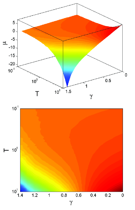
Figure 1: (Color online) Three dimensional illustration of the phase structure in the nonlinear fitness complex network (Top), and its projection on the $\gamma-T$ plane (Bottom). In top panel, it shows the chemical potential $\mu$ as a function of temperature $T$ and the nonlinear exponent $\gamma$, as defined in Eqn. (8). In this simulation we take the number of links per node (per time step) $m=2$, and energy level distribution $g(\varepsilon)=2\varepsilon$ (normalized), and the total number of time steps $t=10^{3}$, average over $100$ runs.

The situation is more clear when we plot the chemical potential $\mu$ as a function of exponent $\gamma$ in Fig. 2, and of temperature $T$ in Fig. 3, respectively. These figures display the different “cross section” views of 3d “phase diagram” of Fig. 1. Some new features of the phase transition can be read out from these plots. In Fig. 2, we show the chemical potential $\mu$ versus the exponent $\gamma$ with temperature $T$ fixed. It can be seen from the figure that as temperature increases, the critical value of exponent for phase transition $\gamma_{C}$ decreases, e.g., for $T=0.2$, $\gamma_{C}\sim 1.2$, while for $T=5.0$, $\gamma_{C}\sim 0.6$, roughly. This tells us that the transition of phase occurs with weaker tendency of preferential linking at relatively higher temperature.

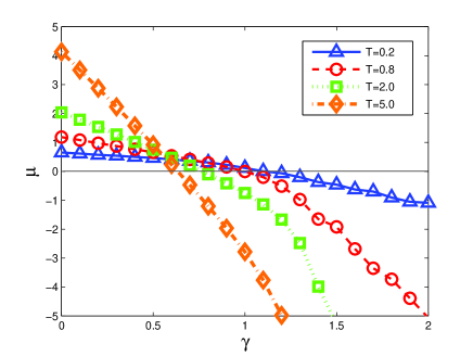
Figure 2: (Color online) The chemical potential $\mu(\gamma,T)$ as a function of the exponent $\gamma$ but with temperature fixed, in a linear-linear scale. The four curves shown in the panel correspond to $T=0.2$ (open triangles, solid line), $T=0.8$ (open circles, dashed line), $T=2.0$ (open squares, dotted line), $T=5.0$ (open diamonds, dot-dashed line), respectively. All symbols are connected by lines for eye guidance.

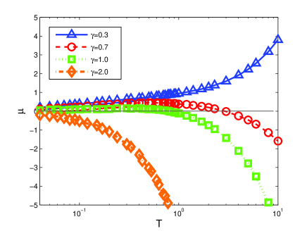
Figure 3: (Color online) Similar to Fig. 2, the chemical potential $\mu(\gamma,T)$ as a function of temperature but with exponent $\gamma$ fixed, in a linear-log scale. The four curves shown in the panel correspond to $\gamma=0.3$ (open triangles, solid line), $\gamma=0.7$ (open circles, dashed line), $\gamma=1.0$ (open squares, dotted line), $\gamma=2.0$ (open diamonds, dot-dashed line), respectively. Note that for $\gamma=0.3$, the values of $\mu$-s are all positive, while for $\gamma=2.0$, the values of $\mu$-s are all negative.

In Fig. 3 we plot the chemical potential $\mu$ versus the temperature $T$ with exponent $\gamma$ fixed in a linear-log scale. For data points with $\gamma=0.7$ (open circles, dashed line) and $\gamma=1$ (open squares, dotted line), the condensation phase transition is very similar to what happens in Fig. 2: the critical temperature $T_{C}$ of the phase transition decreases as the exponent $\gamma$ increases, e.g., for $\gamma=0.7$, $T_{C}\sim 3.0$, while for $\gamma=1$, $T_{C}\sim 0.8$. The latter case recovers the results of B-B BEC phase transition, as it should. Fig. 3 also displays some new, interesting aspects: the values of the chemical potential with $\gamma=0.3$ (open triangles, solid line) are all positive and those with $\gamma=2$ are all negative. This implies that the phase transition disappears eventually as $\gamma$ reaches some specific critical value, and hence results in a single phase structure – either a FGR phase (with negative chemical potential), or a condensation phase (with positive chemical potential). However, one can not always use this as an identification of transition between the condensation phase and the non-condensation phase, this point is illustrated in Fig. 4.

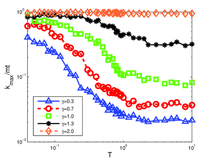
Figure 4: (Color online) The occupation ratios of the most connected node, $k_{max}/mt$, plotted as a function of temperature $T$, and of different nonlinear exponent $\gamma$. The five curves in the panel, from bottom to top, represent $\gamma=0.3$ (open triangles, solid line), $\gamma=0.7$ (open circles, dashed line), $\gamma=1$ (open squares, dotted line), $\gamma=1.3$ (stars, solid line), $\gamma=2$ (open diamonds, dot-dashed line), respectively. Note that the data points with $\gamma=1$ are consistent with B-B’s results (see the corresponding curve of Fig. 3. in Ref. [19]).

We plot the occupation ratio, $k_{max}/mt$, of the most connected node, in Fig. 4. At the first sight from Fig. 4, it seems that the network is in a condensation phase at low enough temperature $T<T_{C}$ ($T_{C}$ is the critical temperature), and in a non-condensation phase at high temperature, $T>T_{C}$. But note that as the exponent $\gamma$ increases, the condensation phase appears in even higher temperature region. Especially when $\gamma=2$, the network enters a condensation phase regardless of the value of temperature. This supports the conclusion of nonlinear growing network in Ref. [18]. However, in addition to the appearance of the condensation phase in original B-B fitness model and the nonlinear model with $\gamma>1$, we conclude from Fig. 4 that they are still different phases because the chemical potential is positive ($\mu>0$) for the B-B fitness model at $T<T_{C}$, while negative ($\mu<0$) for the nonlinear model. The competitive relationship between $e^{-\beta\varepsilon_{i}}$ and $k^{\gamma}$ in partition function play important roles in the dynamical evolution of corresponding complex networks and hence the formation of such a novel phase structure. When the former factor $e^{-\beta\varepsilon_{i}}$ is dominant, the network experiences a condensation phase transition if $T<T_{C}$, and its chemical potential is positive, $\mu>0$; while the prevailing role of the factor $k^{\gamma}$ leads to the opposite side: the chemical potential of the condensation phase is always negative, $\mu<0$. It is also clear that, from above figure, for $\mu>0$ and $\gamma=1$, the network with fitness preferential attachment is condensed on the node with the lowest energy level (or the fittest node) only if $T<T_{C}$ in the thermodynamic limit; for $\mu<0$, the network experiences a “winner takes all” phenomenon when $\gamma$ is large enough (e.g., $\gamma>1.7$). Due to aforementioned competitive relationship between two factors $e^{-\beta\varepsilon_{i}}$ and $k^{\gamma}$, the chemical potential of the non-condensation phase is changed, for instance, see the curve with $\gamma=0.3$ in Fig. 3, though one has an overall positive $\mu$ at high temperature, no condensation phase appears. The different phase structures identified by the chemical potential $\mu$ stem from different dominant factors of preferential attachment mechanism, they are distinct in nature. In addition, as is well known, a significantly different manifestation of BEC and FGR phases is that the fraction of the total number of links connected to the most connected node tends to zero in thermodynamic limit for the latter and tends to a finite value for the former. In current combined model, Fig. 4 shows that there exists a similar situation for $\mu>0$ when the factor $\eta$ dominates the attachment mechanism. while when the factor $\gamma$ dominates the attachment, the ratio tends to zero in thermodynamic limit for $\mu<0$, which displays a FGR phase. However, note that if $\gamma$ is large enough, this occupation ratio can also approach to a finite value and a condensation phase appears even for $\mu<0$.

A major difference between the condensations of fitness model and non-linear model is that the condensation in the former occurs on the node with the lowest energy level (or the highest fitness), instead in the latter model it only occurs on the first node of the network. However, topologically it is hardly able to tell whether or not a graph has reached condensation due to the non-linear preferential attachment or the BEC due to the fitness, since in both condensation phases, the important topological parameter, i.e., the cluster coefficient (CC) approaches to the same limit. If one trace the node with the lowest energy level, then this node is more likely to be the most connected node in low temperature region, since with large parameter $\beta=1/T$, the fitness parameter $\eta$ dominates the dynamical evolution in combined attachment mechanism. As temperature increases, the probability of the node with the lowest energy level being the most connected node is getting smaller due to the impact of fitness $\eta$, as a result, in high temperature region, the factor $k^{\gamma}$ dominates the attachment. This is shown in Fig. 5, in which the occupation ratios of the node with the lowest energy level, $k_{\varepsilon}/mt$, is plotted; as well as that of the most connected node, $k_{max}/mt$, as function of temperature. The former exhibits evidently larger fluctuations compared to the occupation ratio of the most connected node $k_{max}/mt$, since the node with the lowest energy level is not necessary the most connected node. As a result, in high temperature region, in which $k^{\gamma}$ dominates the attachment ($\eta\rightarrow 1$), fluctuations are relatively small, since as a global parameter, $\gamma$ does not depend on the local fitness of a node, such that the earliest presented node could be the most connected node for large $\gamma$, regardless the local fitness for $T>T_{C}$ ($T_{C}$ is the critical temperature); in low temperature region, ($T<T_{C}$), fluctuations of the occupation ratio of a node with the lowest energy level suggests that the emergence of condensation comes from the competition of two sides – the local fittest node (with fitness attachment) and the earliest presented node (with super-linear preferential attachment), and this competition between makes fluctuations larger and larger (e.g., see $\gamma=2$ in Fig. 5). This demonstrates how both attachment factors $\eta$ and $\gamma$ control the evolution of the network simultaneously.

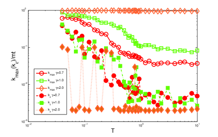
Figure 5: (Color online) The occupation ratios of the most connected node, $k_{max}/mt$, and that of the node with the lowest energy level, $k_{\varepsilon}/mt$, plotted as a function of temperature $T$, and of different nonlinear exponent $\gamma$’s. Data with hollow symbols and solid lines correspond to $k_{max}/mt$, represent $\gamma=0.7$ (open circles), $\gamma=1$ (open squares), $\gamma=2$ (open diamonds), respectively. Data with solid symbols and non-solid lines correspond to $k_{\varepsilon}/mt$, represent $\gamma=0.7$ (solid circles, dashed line), $\gamma=1$ (solid squares, dot-dashed line), $\gamma=2$ (solid diamonds, dotted line), respectively.

4 Conclusions

In conclusion, in this paper we analyze the condensation phase transitions in a unifying framework which includes both the nonlinear model and the fitness model as its appropriate limit. The goodness of this new framework is to, on one hand, bridge the differences between the nonlinear model and the fitness model; On the other hand, allow us to identify the different roles played by different factors in current model. Under appropriate limits (e.g., $\gamma\rightarrow 1$ or $\eta\rightarrow 1$), the typical phase structures of the original B-B fitness model and the nonlinear model are recovered respectively.

Through the numerical simulations of this nonlinear fitness model, we show a novel 3d phase diagram. We employ the Bianconi–Barabàsi method and numerically compute the chemical potential to identify the critical points ($T_{C}$ and $\gamma_{C}$) of the phase transitions of the networks. Our results and analysis directly answer the questions that asked in the beginning, i.e., the condensation phase transitions in both the B-B fitness model and the nonlinear model are in fact distinct in nature. As well, the preferential attachment mechanism in our nonlinear fitness model depends on two factors: $k^{\gamma}$ and $e^{-\beta\varepsilon_{i}}$ (or $\eta_{i}$). Both factors affect the phase structure of the network and hence the network topologies during the evolution of the network. We reveal that the competitive relationship between these two factors leads to the condensation phase transitions, and hence transitions between different network topologies. We hope the current study may increase our understanding to the non-equilibrium critical phenomena, particularly the condensation phase transitions in the evolution of complex networks.

- [1] \NameBose S. N. \REVIEWZeitschrift fur Physik261924178.
- [2] \NameAnderson M. H., Ensher J. R., Matthews M. R., Wieman C. E. Cornell E. A. \REVIEWScience2691995198.
- [3] \NameBradley C. C., SackettC. A., Tollett J. J. Hulet R. G. \REVIEWPhys. Rev. Lett.7519951687.
- [4] \NameEvans M. R. \REVIEWEurophys. Lett.36199613.
- [5] \NameChowdhury D., Santen L. Schadschneider A. \REVIEWPhys. Rep.3292000199.
- [6] \NameBurda Z., Johnston D., Jurkiewicz J., Kamiński M., Nowak M. A., Papp G., Zahed I. \REVIEWPhys. Rev. E652002026102.
- [7] \NameEvans M. R., Hanney T. \REVIEWJ. Phys. A: Math. Gen.382005R195.
- [8] \NameWatts D. J. Strogatz S. H. \REVIEWNature3931998440.
- [9] \NameBarabási A.-L. Albert R. \REVIEWScience2861999509.
- [10] \NameBarabási A.-L., Albert R. Jeong H. \REVIEWPhysica A (Amsterdam)281200069.
- [11] \NameStrogatz S. H. \REVIEWNature4102001268.
- [12] \NameDorogovtesev S. N. Mendes J. F. F. \REVIEWAdv. Phys.5120021079.
- [13] \NameNewman M. E. J. \REVIEWSIAM Rev.452003167.
- [14] \NameWatts D. J. \BookSmall Worlds: The Dynamics of Networks between Order and Randomness \PublPrinceton University Press, Princeton, NJ \Year1999.
- [15] \NamePastor-Satorras R. Vespignani A. \BookEvolution and Structure of the Internet: A Statistical Physics Approach \PublCambridge University Press, Cambridge \Year2004.
- [16] \NameDorogovtesev S. N. Mendes J. F. F. \BookEvolution of Networks: From Biological Nets to the Internet and WWW \PublOxford University Press, Oxford \Year2003.
- [17] \NameBouchaud J. P. Mézard M. \REVIEWPhysica A2822000536.
- [18] \NameKrapivsky P. L., Redner S. Leyvraz F. \REVIEWPhys. Rev. Lett.8520004629.
- [19] \NameBianconi G. Barabási A.-L. \REVIEWPhys. Rev. Lett.8620015632.
- [20] \NameBurda Z., Correia J. D. Krzywicki A. \REVIEWPhys. Rev. E642001046118.
- [21] \NameGodréche C. Luck J. M. \REVIEWEur. Phys. Jour. B232001473.
- [22] \NameBauer M. Bernard D. arXiv:cond-mat/0206150.
- [23] \NameBerg J. Lässig M. \REVIEWPhys. Rev. Lett.892002228701.
- [24] \NameErgün G. Rodgers G. J. \REVIEWPhysica A3032002261.
- [25] \NameDorogovtesev S. N., Mendes J. F. F. Samukhin A. N. \REVIEWNucl. Phys. B6532003307.
- [26] \NameDorogovtesev S. N., Mendes J. F. F., Povolotsky A. M. Samukhin A. N. \REVIEWPhys. Rev. Lett.952005195701.
- [27] \NameDorogovtesev S. N., Mendes J. F. F., Povolotsky A. M. Samukhin A. N. \REVIEWNucl. Phys. B6662003396.
- [28] \NameFarkas I., Derenyi I., Palla G. Vicsek T. \REVIEWLect. Notes Phys.6502004163.
- [29] \NameGodréche C. Luck J. M. \REVIEWJ. Phys. A: Math. Gen.3820057215.
- [30] \NameNoh J. D., Shim G. M. Lee H. \REVIEWPhys. Rev. Lett.942005198701.
- [31] \NameNoh J. D. \REVIEWPhys. Rev. E722005056123.
- [32] \NameOhkubo J. Horiguchi T. \REVIEWJ. Phys. Soc. Jpn.7420051334.
- [33] \NameOhkubo J., Tanaka K. Horiguchi T. \REVIEWPhys. Rev. E722005036120.
- [34] \NameOhkubo J., Yasuda M. Tanaka K. \REVIEWPhys. Rev. E722005065104(R).
- [35] \NameOhkubo J. arXiv: 0707.4519v2.
- [36] \NameBialas P., Burda Z. Johnston D. \REVIEWNucl. Phys. B4931997505.
- [37] \NameBianconi G. Barabási A.-L. \REVIEWEurophys. Lett.542001436.
- [38] \NameBarabási A.-L. Albert R. \REVIEWRev. Mod. Phys.74200247.
- [39] \NameGoltsev A. V., Dorogovtesev S. N. Mendes J. F. F. \REVIEWRev. Mod. Phys.8020081275.