Two-band model of Raman scattering on iron pnictide superconductors

Abstract

Based on a two-band model, we study the electronic Raman scattering intensity in both normal and superconducting states of iron-pnictide superconductors. For the normal state, due to the match or mismatch of the symmetries between band hybridization and Raman vertex, it is predicted that overall $B_{1g}$ Raman intensity should be much weaker than that of the $B_{2g}$ channel. Moreover, in the non-resonant regime, there should exhibit a interband excitation peak at frequency $\omega\simeq 7.3t_{1}(6.8t_{1})$ in the $B_{1g}$ ($B_{2g}$) channel. For the superconducting state, it is shown that $\beta$-band contributes most to the $B_{2g}$ Raman intensity as a result of multiple effects of Raman vertex, gap symmetry, and Fermi surface topology. Both extended $s$- and $d_{xy}$-wave pairings in the unfolded BZ can give a good description to the reported $B_{2g}$ Raman data [Muschler et al., Phys. Rev. B. 80, 180510 (2009).], while $d_{x^{2}-y^{2}}$-wave pairing in the unfolded BZ seems to be ruled out.

I Introduction

Recently superconductivity has been observed in several classes of iron-pnictide materials. kamihara ; Wang08 ; Hsu Despite that different classes of pnictides have somewhat different crystal structures, their electronic structures behave to be quite similar, as confirmed by ARPES and magneto-oscillation measurements. Liu177005 ; Evtushinsky ; Coldea Band structure calculations indicate that iron pnictides exhibit a quasi-two-dimensional electronic structure. Their parent compounds are metals which display an antiferromagnetic long-range order. Superconductivity is induced either by hole doping or electron doping when part of $\mathrm{Fe}^{2+}$ ions are replaced by $\mathrm{Fe}^{+}$, or solely by the application of high pressure. Overall speaking, iron-pnictide shows a good resemblance with the high-$T_{c}$ cuprate superconductor, and hence is an ideal candidate for studying the superconducting (SC) mechanism of high $T_{c}$.

One crucial issue towards identifying the interaction that drives superconductivity is the symmetry structure of Cooper pairs. A conclusive observation of the pairing symmetry remains unsettled for iron pnictides, however, Both nodal and nodeless order parameters were reported in experimental observations. ARPES measurements clearly indicated a nodeless gap at all points of the Fermi surface. Ding_EPL ; zhao Moreover, magnetic penetration depth measurement has revealed a $T^{2}$ behavior down to $0.02T_{c}$ – a possible signature for the unconventional $s_{\pm}$ state.mazin:057003 The $s_{\pm}$ state is currently a promising pairing candidate for iron pnictides, which has a sign reversal between $\alpha$ and $\beta$ bands and can be naturally explained by the spin fluctuation mechanism. mazin:057003 ; wang:047005 ; Tsuei2010 On the other hand the neutron-scattering spectrum seems to suggest the order parameter being fully gapped but without a sign reversal (called $s_{++}$-wave in contrast to $s_{\pm}$-wave). PhysRevB.81.060504 ; PhysRevB.81.180505 On the contrary, both scanning SQUID microscopyhicks-2008 and NMR measurements Matano ; Grafe08 are in favor of nodal SC order parameters. For phase sensitive experiments however, one point-contact spectroscopy reported was in favor of a nodal gap Shan , while the others reported were in favor of a nodeless gap. chen

Compared to other spectroscopy experiments, Raman scattering has a unique feature, namely, by manipulating the polarization directions of incident and scattered photons with respect to the crystallographic directions, it can selectively excite quasiparticles (QPs) on different parts of the Brillouin zone (BZ) . Therefore Raman scattering is considered a very useful probe for studying pairing symmetry of the SC order parameter. More explicitly, among various symmetry channels ($A_{1g}$, $A_{2g}$, $B_{1g}$, and $B_{2g}$ within a $D_{\rm 4h}$ symmetry group), powers laws of low-energy Raman intensity as well as peak positions can often give useful information on the pairing symmetry of a superconductor. Raman scattering had been very successful on the studies of the high-$T_{c}$ cuprate superconductors. RevModPhys.79.175 It is also anticipated that Raman scattering will give very useful signals on the iron-pnictide superconductors.

Electronic Raman scattering experiment has recently been carried out on high-quality single-crystal Ba(Fe_1-xCo_x)₂As₂. PhysRevB.80.180510 Both normal- and superconducting-state data were taken and for frequency below 300 cm^-1, it showed that a significant change of the Raman response between the normal and superconducting state occurs only in the $B_{2g}$ channel to which a strong peak develops at $\omega=69$cm^-1 in the superconducting state. Moreover, the low-energy spectral weight in the SC state suggests a gap having nodes for certain doping levels of Ba(Fe_1-xCo_x)₂As₂. It is of importance to perform a more quantitative theoretical fitting on the Raman data reported in Ref. [PhysRevB.80.180510, ] and this is indeed the goal of the present paper.

On the theoretical side, Boyd et al. PhysRevB.79.174521 have calculated the Raman response for iron-pnictides taking into account multiple gaps on different Fermi sheets. In their calculations, the Raman vertices are obtained by the expansion of harmonic functions for a cylindrical FS and the screening effect due to the long-range Coulomb interaction is considered but leaving out vertex corrections capturing effects of final state interactions. Their results give a criterion to distinguish the momentum and frequency dependence of the SC order parameters by Raman scattering. In another study, Chubukov and coworkers PhysRevB.79.220501 ; Physics.2.46 have also calculated the Raman response for iron-pnictide superconductors. By analyzing the vertex corrections for the extended $s$-wave gap symmetry, they have revealed a collective mode below $2\Delta_{0}$ in the $A_{1g}$ channel that may be crucial to unravel the pairing symmetry. It provides an alternative way to distinguish between various suggested gap symmetries of the iron-pnictide superconductors.

The electronic structure of iron-pnictide materials is considered to be more complex than that of the high-T_c cuprates. The band structure calculations showed that superconductivity is associated with the Fe-pnictide layer, and the FS consists of two hole pockets and two electron pockets. singh:237003 ; PhysRevB.77.220506 The maximum contribution to the density of states near the FS is due to the Fe-3$d$ orbitals. Several tight-binding models are thus proposed to construct the band structure and several competing orders are suggested to exist in these materials. PhysRevB.77.220506 ; PhysRevLett.101.087004 ; PhysRevLett.101.057008 ; 0953-8984-20-42-425203 In this paper, we shall study the Raman response based on a two-band model.raghu_prb_08 This minimal model is considered to be a promising one which captures the major features of the electronic structures of several classes of iron-pnictide materials. As mentioned before, our aim is to give a more quantitative fitting to the current available Raman data and uncover useful fitting parameters. It is hoped that our study, together with other theoretical Raman works (Refs. PhysRevB.79.220501, ; PhysRevB.79.174521, ) can give a more complete picture on the pairing symmetry and electronic structure of iron pnictides.

The paper is organized as the following. In Sec. II, we present the two-band model Hamiltonian for iron-pnictide superconductors. In Sec. III, theoretical derivations are given for the Raman scattering both in the normal and in the SC states with respect to the two-band model given in Sec. II. Calculations of Raman response are presented for both normal and SC states. Some predictions are made. Especially fitting to the $B_{2g}$ Raman peak in the SC state are performed with useful fitting parameters given. Sec. IV is a summary of this paper.

II Model Hamiltonian

For iron-pnictides, we start from the minimal two-band model introduced in Ref. [raghu_prb_08, ]. The normal-state Hamiltonian reads as

$$H_{0}=\sum_{\mathbf{k}\sigma}\left(\begin{array}[]{cc}c_{\mathbf{k}\sigma}^{{\dagger}}&d_{\mathbf{k}\sigma}^{{\dagger}}\end{array}\right)\left(\begin{array}[]{cc}\varepsilon_{x}-\mu&\varepsilon_{xy}\\ \varepsilon_{xy}&\varepsilon_{y}-\mu\end{array}\right)\left(\begin{array}[]{c}c_{\mathbf{k}\sigma}\\ d_{\mathbf{k}\sigma}\end{array}\right),$$ (1)

where $\mu$ is the chemical potential and $(c_{\mathbf{k}\sigma}^{(\dagger)},d_{\mathbf{k}\sigma}^{(\dagger)})$ are annihilation (creation) operators that annihilate (create) an electron in the $d_{xz}$- and $d_{yz}$-orbital with spin $\sigma$ and wavevector $\mathbf{k}$, respectively. Energy dispersions of orbital $d_{xz}$ and $d_{yz}$ are given by $\varepsilon_{x}=-2t_{1}\cos k_{x}-2t_{2}\cos k_{y}-4t_{3}\cos k_{x}\cos k_{y}$ and $\varepsilon_{y}=-2t_{2}\cos k_{x}-2t_{1}\cos k_{y}-4t_{3}\cos k_{x}\cos k_{y}$ respectively, which are coupled by the $d_{xy}$ orbital with dispersion $\varepsilon_{xy}=-4t_{4}\sin k_{x}\sin k_{y}$. By the unitary transformation

$$\left(\begin{array}[]{c}c_{\mathbf{k}\sigma}\\ d_{\mathbf{k}\sigma}\end{array}\right)=\left(\begin{array}[]{cc}\cos\theta_{\mathbf{k}}&-\sin\theta_{\mathbf{k}}\\ \sin\theta_{\mathbf{k}}&\cos\theta_{\mathbf{k}}\end{array}\right)\left(\begin{array}[]{c}\alpha_{\mathbf{k}\sigma}\\ \beta_{\mathbf{k}\sigma}\end{array}\right),$$ (2)

Hamiltonian (1) can be transformed to

$$H_{0}=\sum_{\mathbf{k}\sigma}\left(\begin{array}[]{cc}\alpha_{\mathbf{k}\sigma}^{{\dagger}}&\beta_{\mathbf{k}\sigma}^{{\dagger}}\end{array}\right)\left(\begin{array}[]{cc}E_{-}&0\\ 0&E_{+}\end{array}\right)\left(\begin{array}[]{c}\alpha_{\mathbf{k}\sigma}\\ \beta_{\mathbf{k}\sigma}\end{array}\right),$$ (3)

where $E_{\pm}=\varepsilon_{+}\pm\sqrt{\varepsilon_{-}^{2}+\varepsilon_{xy}^{2}}-\mu$ with $\varepsilon_{\pm}\equiv\left(\varepsilon_{x}\pm\varepsilon_{y}\right)/2$. The new basis $(\alpha_{\mathbf{k}\sigma},\beta_{\mathbf{k}\sigma})$ consists of new fermionic QP operators in the $E_{\pm}$ bands which are hybrids of the $d_{xz}$- and $d_{yz}$-orbital. In the literature, $E_{-}$ ($E_{+}$) is usually labeled as the $\alpha$ ($\beta$) band.

The coherence factors in (2) can be solved to be

$$\cos^{2}\theta_{\mathbf{k}} = \frac{1}{2}\left(1+\frac{\varepsilon_{\mathbf{-}}}{\sqrt{\varepsilon_{xy}^{2}+\varepsilon_{\mathbf{-}}^{2}}}\right)$$

$$\sin^{2}\theta_{\mathbf{k}} = \frac{1}{2}\left(1-\frac{\varepsilon_{\mathbf{-}}}{\sqrt{\varepsilon_{xy}^{2}+\varepsilon_{\mathbf{-}}^{2}}}\right).$$ (4)

Moreover, the single-particle Matsubara Green’s functions in the normal-state are

$$\mathcal{G}^{0}_{cc}(\mathbf{k},ip_{n}) = -\int_{0}^{\beta}d\tau~{}e^{ip_{n}\tau}\langle c_{{\bf k}\sigma}(\tau)c^{\dagger}_{{\bf k}\sigma}(0)\rangle_{0}$$

$$= \frac{\cos^{2}\theta_{\mathbf{k}}}{ip_{n}-E_{-}}+\frac{\sin^{2}\theta_{\mathbf{k}}}{ip_{n}-E_{+}},$$

$$\mathcal{G}^{0}_{dd}(\mathbf{k},ip_{n}) = -\int_{0}^{\beta}d\tau~{}e^{ip_{n}\tau}\langle d_{{\bf k}\sigma}(\tau)d^{\dagger}_{{\bf k}\sigma}(0)\rangle_{0}$$ (5)

$$= \frac{\sin^{2}\theta_{\mathbf{k}}}{ip_{n}-E_{-}}+\frac{\cos^{2}\theta_{\mathbf{k}}}{ip_{n}-E_{+}},$$

$$\mathcal{G}^{0}_{cd}(\mathbf{k},ip_{n}) = \mathcal{G}^{0}_{dc}(\mathbf{k},ip_{n})=-\int_{0}^{\beta}d\tau~{}e^{ip_{n}\tau}\langle c_{{\bf k}\sigma}(\tau)d^{\dagger}_{{\bf k}\sigma}(0)\rangle_{0}$$

$$= -\frac{\sin 2\theta_{\mathbf{k}}}{2}\left(\frac{1}{ip_{n}-E_{-}}-\frac{1}{ip_{n}-E_{+}}\right).$$

Throughout this paper, we shall choose $t_{1}=-1$, $t_{2}=1.3$, $t_{3}=t_{4}=-0.85$, and $\mu=1.54$, all measured in units of $|t_{1}|$. These represent a good fit to the first-principle calculations for the band structures of LaOFeAs. Xu67002

III Raman Scattering

III.1 Normal state

Raman scattering intensity is proportional to the imaginary part of the effective density-density correlation function $\chi(\mathbf{q},\tau)=\langle T_{\tau}[\tilde{\rho}(\mathbf{q},\tau),\tilde{\rho}(-\mathbf{q},0)]\rangle$ in the $\mathbf{q}\rightarrow 0$ limit. For the current two-band system, effective density operator associated with Raman scattering can be given by

$$\tilde{\rho}(\mathbf{q},\tau) \equiv {\sum_{\mathbf{k}\sigma}}[\gamma_{\mathbf{k}}^{c}c_{\mathbf{k}+\mathbf{q}\sigma}^{{\dagger}}(\tau)c_{\mathbf{k}\sigma}(\tau)$$ (6)

$$+ \gamma_{\mathbf{k}}^{d}d_{\mathbf{k}+\mathbf{q}\sigma}^{{\dagger}}(\tau)d_{\mathbf{k}\sigma}(\tau)],$$

where $\gamma_{\mathbf{k}}^{c}$ ($\gamma_{\mathbf{k}}^{d}$) is the Raman vertex associated with the electrons on $d_{xz}$ ($d_{yz}$) orbital. In the Matsubara frequency space, symmetry-channel dependent irreducible Raman response function in the normal state has been solved to be

$$\chi_{N}({\bf q}\rightarrow 0,i\omega_{n})={1\over 4}\sum_{\mathbf{k}}\Gamma_{\mathbf{k}}^{2}$$ (7)

$$\times\left[\frac{f(E_{-})-f(E_{+})}{i\omega_{n}-(E_{+}-E_{-})}+\frac{f(E_{+})-f(E_{-})}{i\omega_{n}-(E_{-}-E_{+})}\right],$$

where $f(E)=1/[\exp(E/{k_{B}T})+1]$ is the Fermi distribution function and

$$\Gamma_{\mathbf{k}}=\sin 2\theta_{\mathbf{k}}\left(\gamma_{\mathbf{k}}^{c}+\gamma_{\mathbf{k}}^{d}\right)$$ (8)

is a weighting factor for the symmetry-dependent Raman scattering of a two-band system. $\Gamma_{\mathbf{k}}$ is comprised of two parts where $\sin 2\theta_{\mathbf{k}}$ corresponds to the effect of orbital hybridization, while $(\gamma_{\mathbf{k}}^{c}+\gamma_{\mathbf{k}}^{d})$ is the sum of the Raman vertexes associated with two individual orbitals. In the case of zero orbital hybridization ($\varepsilon_{xy}\rightarrow 0$), $\sin 2\theta_{\mathbf{k}}\rightarrow 0$ and hence $\chi_{N}\rightarrow 0$.

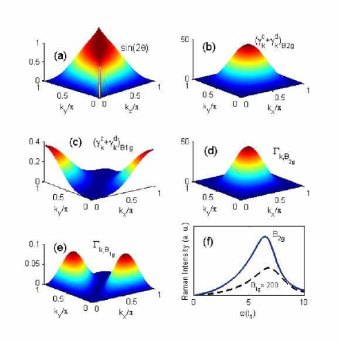
Figure 1: (Color online) Panel (a)–(e): To see the properties of the channel-dependent weighting factor $\Gamma_{\mathbf{k}}$, $\sin 2\theta_{\mathbf{k}}$, $(\gamma_{\mathbf{k}}^{c}+\gamma_{\mathbf{k}}^{d})_{B_{2g}}$, $(\gamma_{\mathbf{k}}^{c}+\gamma_{\mathbf{k}}^{d})_{B_{1g}}$, $\Gamma_{\mathbf{k},B_{2g}}$, and $\Gamma_{\mathbf{k},B_{1g}}$ are plotted respectively in the first quadrant of the BZ. Panel (f) is the calculated normal-state Raman intensity.

When the energy of incident light is much smaller than the optical band gap of the system, the contribution from the resonant channel is negligible. Consequently, Raman vertex can be obtained in terms of the curvature of the band dispersion, known as the inverse effective mass approximation.PhysRevB.51.16336 That is, depending on the symmetry of the Raman modes, $(\gamma_{\mathbf{k}}^{c})_{ij}\sim\partial^{2}\varepsilon_{x}/\partial{\bf k}_{i}\partial{\bf k}_{f}$ and $(\gamma_{\mathbf{k}}^{d})_{ij}\sim\partial^{2}\varepsilon_{y}/\partial{\bf k}_{i}\partial{\bf k}_{f}$ with ${\bf k}_{i}$ and ${\bf k}_{f}$ being the wavevectors of incident and scattered lights respectively. In the current two-band model of iron-pnictides, it is obtained that

$$(\gamma_{\mathbf{k}}^{c})_{B_{1g}} \sim \frac{1}{2}(\varepsilon_{x}^{xx}-\varepsilon_{x}^{yy})=t_{1}\cos{k}_{x}-t_{2}\cos{k}_{y},$$

$$(\gamma_{\mathbf{k}}^{d})_{B_{1g}} \sim \frac{1}{2}(\varepsilon_{y}^{xx}-\varepsilon_{y}^{yy})=t_{2}\cos{k}_{x}-t_{1}\cos{k}_{y},$$ (9)

$$(\gamma_{\mathbf{k}}^{c})_{B_{2g}} = (\gamma_{\mathbf{k}}^{d})_{B_{2g}}\sim\varepsilon_{x}^{xy}=\varepsilon_{y}^{xy}=4t_{3}\sin{k}_{x}\sin{k}_{y},$$

where $\varepsilon_{x}^{xx}\equiv\partial^{2}\varepsilon_{x}/\partial{\bf k}_{x}\partial{\bf k}_{x}$, etc.

In Fig. 1, we first examine the behaviors of the weighting factor $\Gamma_{\mathbf{k}}$. Respectively in Fig. 1(a)–(e), we plot $\sin 2\theta_{\mathbf{k}}$, $(\gamma_{\mathbf{k}}^{c}+\gamma_{\mathbf{k}}^{d})_{B_{2g}}$, $(\gamma_{\mathbf{k}}^{c}+\gamma_{\mathbf{k}}^{d})_{B_{1g}}$, $\Gamma_{\mathbf{k},B_{2g}}$, and $\Gamma_{\mathbf{k},B_{1g}}$ in the first quadrant of the BZ. As shown, both $\sin 2\theta_{\mathbf{k}}$ and $(\gamma_{\mathbf{k}}^{c}+\gamma_{\mathbf{k}}^{d})_{B_{2g}}$ are peaked at $(\pi/2,\pi/2)$, while $(\gamma_{\mathbf{k}}^{c}+\gamma_{\mathbf{k}}^{d})_{B_{1g}}$ is peaked at $(\pi,0)$ and $(0,\pi)$. Consequently, $\Gamma_{\mathbf{k},B_{2g}}$ is strongly peaked at $(\pi/2,\pi/2)$, while due to the mismatch of $\sin 2\theta_{\mathbf{k}}$ and $(\gamma_{\mathbf{k}}^{c}+\gamma_{\mathbf{k}}^{d})_{B_{1g}}$, $\Gamma_{\mathbf{k},B_{1g}}$ turns out to have two peaks located at $(k_{x},k_{y})=(0.26\pi,0.74\pi)$ and $(0.74\pi,0.26\pi)$. The symmetry mismatch between $\sin 2\theta_{\mathbf{k}}$ and $(\gamma_{\mathbf{k}}^{c}+\gamma_{\mathbf{k}}^{d})_{B_{1g}}$ implies that the overall normal-state $B_{1g}$ Raman intensity should be weaker than that of the $B_{2g}$ channel. The reported normal-state Raman intensities of Ba(Fe_1-xCo_x)₂As₂ seem to be consistent with the prediction. PhysRevB.80.180510

Fig. 1(f) shows the calculated normal-state Raman spectra in both $B_{1g}$ and $B_{2g}$ channels. Apart from the feature that $B_{1g}$ Raman intensity is much weaker than that of the $B_{2g}$ channel, $B_{2g}$-channel Raman intensity shows a peak at $\omega\simeq 6.8t_{1}$ while $B_{1g}$-channel Raman intensity shows a peak at $\omega\simeq 7.3t_{1}$. According to Eq. (7), the frequencies where the peaks appear are actually predictable. When temperature $T\rightarrow 0$, the Raman peak for each channel can be estimated to be at $\omega=E_{+}(k_{x},k_{y})-E_{-}(k_{x},k_{y})$ with $(k_{x},k_{y})$ corresponding to the maximum of the weighting factor $\Gamma_{\bf k}$. Therefore for $B_{2g}$-channel Raman intensity, the peak is predicted to be at $\omega=E_{+}(\pi/2,\pi/2)-E_{-}(\pi/2,\pi/2)=6.8t_{1}$, while the $B_{1g}$-channel Raman peak is predicted to be at $\omega=E_{+}(0.74\pi,0.26\pi)-E_{-}(0.74\pi,0.26\pi)=7.3t_{1}$. The above predicted normal-state Raman peaks may provide an alternative route to the measurement of the band energy scale for iron-pnictide superconductors.

In iron-pnictide superconductors, the energy scale of the nearest hopping $t_{1}$ is estimated to be about $0.05-0.3$eV. Thus the predicted normal-state Raman peaks could have energy $\omega\sim 0.35-2.1$eV. The lower-bound energy (0.35 eV) should well be in the non-resonant regime, while the upper-bound energy (2.1 eV) could be in the resonant regime and poses a question mark for the above results to be valid. Current reported normal-state Raman data on BaFe_1-xCo_x)₂As₂ have only be measured up to 300cm^-1 however. PhysRevB.80.180510

III.2 Superconducting state

We next study the Raman spectra in the SC state. To do so, in a mean-field level one can add a SC pairing Hamiltonian:

$$H_{\text{SC}}\ =\sum_{\mathbf{k}}\left(\Delta_{\mathbf{k}}^{\alpha}\alpha_{\mathbf{k}\uparrow}^{{\dagger}}\alpha_{-\mathbf{k}\downarrow}^{{\dagger}}+\Delta_{\mathbf{k}}^{\beta}\beta_{\mathbf{k}\uparrow}^{{\dagger}}\beta_{-\mathbf{k}\downarrow}^{{\dagger}}+\text{h.c.}\right)$$ (10)

to the diagonalized Hamiltonian $H_{0}$ in (3). In Eq. (10), the pairing is considered between the long-lived $\alpha_{\mathbf{k}\sigma}$ QPs and between $\beta_{\mathbf{k}\sigma}$ QPs only. That is, interband pairing is neglected. Since decoupled $\alpha$ and $\beta$ bands are originated from the coupled $d_{xz}$ and $d_{yz}$-orbitals, the kind of SC pairing Hamiltonian (10) automatically includes both intra- and inter-orbital pairings in the original fermion basis $\left(c_{\mathbf{k}\sigma},d_{\mathbf{k}\sigma}\right)$. PhysRevB.79.020501 ; Nazario:144513 The QP excitation energy is then given by $\tilde{E}_{\mathbf{k}l}=(E^{2}_{l}+|\Delta_{\mathbf{k}}^{l}|^{2})^{1/2}$ ($l=\alpha,\beta$) for the two bands respectively. In this section, for convenience, $E_{-}\rightarrow E_{\alpha}$ and $E_{+}\rightarrow E_{\beta}$.

If the pairing originates from the same mechanism, most likely $\alpha_{1}$ and $\alpha_{2}$ bands will have the same pairing symmetry. Similarly $\beta_{1}$ and $\beta_{2}$ bands will also likely have the same pairing symmetry. The Raman spectra reported in Ref. [PhysRevB.80.180510, ] do not show a clear activation threshold rather exhibit a finite intensity down to an arbitrarily small Raman shift. It gives a strong evidence that the SC pairing favors an anisotropic nodal gap rather than a full isotropic gap such as the $s_{\pm}$ state or the $s_{++}$ state. Furthermore, the scanning SQUID microscopy measurements seemed to exclude the spin-triplet pairing states and suggested that the order parameter has well-developed nodes [hicks-2008, ]. Within the anisotropic and nodal scenarios, the possible candidates are the extended $s$-wave and $d$-wave states.

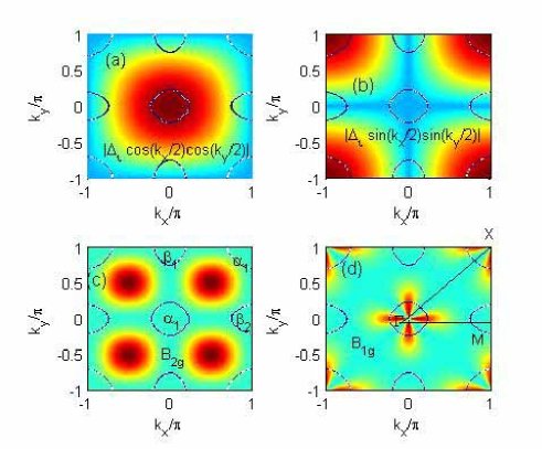
Figure 2: (Color online) Panel (a)&(b): Schematic plot of the $\alpha$- and $\beta$-band Fermi surfaces and the $\mathbf{k}$-dependent amplitude of (a) extended $s$-wave gap and (b) $d_{xy}$-wave gap. Panel (c)&(d): Momentum dependence of the effective Raman vertices of (c) $(\gamma_{\bf k}^{\alpha\alpha})_{B_{2g}}$ and (d) $(\gamma_{\bf k}^{\alpha\alpha})_{B_{1g}}$. Here we only show $(\gamma_{\bf k}^{\alpha\alpha})_{B_{2g}}$ and $(\gamma_{\bf k}^{\alpha\alpha})_{B_{1g}}$ because $(\gamma_{\bf k}^{\beta\beta})_{B_{2g}}=(\gamma_{\bf k}^{\alpha\alpha})_{B_{2g}}$ and $(\gamma_{\bf k}^{\beta\beta})_{B_{1g}}\simeq(\gamma_{\bf k}^{\alpha\alpha})_{B_{1g}}$ (see text).

After a lengthy derivation, the irreducible Raman response function in the SC state is solved to be

$$\chi_{S}(\mathbf{q}\rightarrow 0,\tau) = -\sum_{\mathbf{k},ll^{\prime}=\alpha,\beta}(\gamma_{\mathbf{k}}^{ll^{\prime}})^{2}[\mathcal{G}_{l}(\mathbf{k},\tau)\mathcal{G}_{l^{{}^{\prime}}}(\mathbf{k},-\tau)$$ (11)

$$+ \mathcal{F}_{l}(\mathbf{k},\tau)\mathcal{F}_{l^{{}^{\prime}}}(\mathbf{k},-\tau)],$$

where $\mathcal{G}_{l}$ and $\mathcal{F}_{l}$ are the usual normal and anomalous Green functions for a superconductor associated with band $l$. The intra- and interband vertex functions are solved to be

$$\gamma_{\mathbf{k}}^{\alpha\alpha} =\gamma_{\mathbf{k}}^{c}\cos^{2}\theta_{\mathbf{k}}+\gamma_{\mathbf{k}}^{d}\sin^{2}\theta_{\mathbf{k}},$$

$$\gamma_{\mathbf{k}}^{\beta\beta} =\gamma_{\mathbf{k}}^{c}\sin^{2}\theta_{\mathbf{k}}+\gamma_{\mathbf{k}}^{d}\cos^{2}\theta_{\mathbf{k}},$$ (12)

$$\gamma_{\mathbf{k}}^{\alpha\beta} =\gamma_{\mathbf{k}}^{\beta\alpha}=\sin 2\theta_{\mathbf{k}}(\gamma_{\mathbf{k}}^{c}+\gamma_{\mathbf{k}}^{d})/2,$$

where $\gamma_{\mathbf{k}}^{c}$ and $\gamma_{\mathbf{k}}^{d}$ were defined in (9) for both $B_{1g}$ and $B_{2g}$ channels. Frequency and channel-dependent Raman intensity is proportional to the imaginary part of the effective density-density correlation function (11) transformed to the Matsubara space. As shown in Eq. (11), Raman spectra are contributed by both intraband and interband transitions. Nevertheless, due to the little nesting effect occurring across different bands, interband transitions are negligibly small for the Raman intensity. Thus one can safely ignore the interband Raman scattering in the present case. Consequently, at $T\rightarrow 0$, Raman intensity is proportional to

$$I(\omega)=\sum_{\mathbf{k},l=\alpha,\beta}(\gamma_{\bf k}^{ll})^{2}\left({|\Delta_{\mathbf{k}}^{l}|\over 2\tilde{E}_{\mathbf{k}l}}\right)^{2}\frac{\Gamma}{(\omega-2\tilde{E}_{\mathbf{k}l})^{2}+\Gamma^{2}},$$ (13)

where $\Gamma$ is the broadening which is set to be 0.08 in our calculations.

As is well-known, Raman scattering is a directional probe for SC QP excitations. In the present two-band iron-pnictide superconductors, the directional selectivity is dependent of two factors [see (13)]. One is due to the Raman vertex $\gamma_{\bf k}^{ll}$ and the other is due to the symmetry of the pairing gap $\Delta_{\mathbf{k}}^{l}$. The overall Raman will also depend on the detailed locations and topology of the Fermi surfaces of the system. It is worth noting that, as shown explicitly in (13), Raman intensity is directly proportional to the gap maximum of the pairing gap.

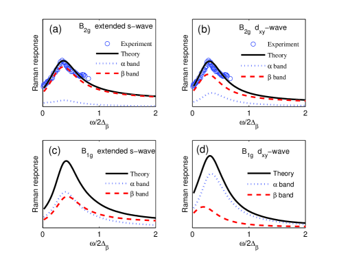
Figure 3: Frame (a) and (b): Comparison of theoretical fitting and experimental data of the $B_{2g}$ Raman spectra. The SC gaps tested are extended $s$-wave $\Delta_{\bf k}=\Delta_{0}\cos k_{x}/2\cos k_{y}/2$ in (a) and extended $d$-wave $\Delta_{\bf k}=\Delta_{0}\sin k_{x}\sin k_{y}$ in (b). Frame (c) and (d) are the calculated $B_{1g}$ Raman shift using the same parameters in frame (a) and (b).

It is important to first observe how the directional selection occurs for the iron-pnictide superconductors. We consider the unfolded BZ for the case of one Fe/cell. The $\alpha$-band FSs of the 2-orbital model are hole Fermi pockets given by $E_{-}(\mathbf{k}_{f})=0$ which are around the $\Gamma$ point and the corner, $(\pm\pi,\pm\pi)$. The $\beta$-band FSs are electron Fermi pockets given by $E_{+}(\mathbf{k}_{f})=0$ which are around the $M$ point. In the SC state. the coupling of the two orbitals results in complex Raman vertices given in (12). Shown in Fig. 2 (c) and (d) are the momentum dependence of the Raman vertices $(\gamma_{\bf k}^{\alpha\alpha})_{B_{2g}}$ and $(\gamma_{\bf k}^{\alpha\alpha})_{B_{1g}}$. Note that for the current two-band model, $(\gamma_{\bf k}^{\beta\beta})_{B_{2g}}=(\gamma_{\bf k}^{\alpha\alpha})_{B_{2g}}$ and $(\gamma_{\bf k}^{\beta\beta})_{B_{1g}}\simeq(\gamma_{\bf k}^{\alpha\alpha})_{B_{1g}}$. It is because $(\gamma_{\bf k}^{c})_{B_{2g}}=(\gamma_{\bf k}^{d})_{B_{2g}}$ and $(\gamma_{\bf k}^{c})_{B_{1g}}\simeq(\gamma_{\bf k}^{d})_{B_{1g}}$ [see Eqs. (9) and (12)] for the current parameters. As shown in Fig. 2 (c) and (d), $B_{2g}$ vertex peaks at $(\pm\pi/2,\pm\pi/2)$ in the unfolded BZ and the peak is roughly of same distance to both $\alpha$- and $\beta$-band FSs. As a matter of the fact, it couples roughly equal to both $\alpha$ and $\beta$ bands. In contrast, the $B_{1g}$ vertex has a $d_{x^{2}-y^{2}}$ symmetry and is centered around the $\Gamma$ point and the corners, $(\pm\pi,\pm\pi)$. Thus it couples predominantly to the $\alpha$ bands in the unfolded BZ. Consequently $B_{1g}$ Raman scattering mainly excite the QP in the $\alpha$ bands and can give more information about the pairing symmetry in the $\alpha$ bands.

We now test the possible extended $s$-wave and $d$-wave pairings. Our approach is the following. We will try to fit the currently available $B_{2g}$ Raman intensity PhysRevB.80.180510 for each possible pairing symmetry. The best fitting parameters of the gap magnitudes will be quoted. Using the best fitting parameters for $B_{2g}$ Raman spectra, the predicted $B_{1g}$ Raman intensity will be given. While $B_{1g}$ Raman intensity is also reported in Ref. [PhysRevB.80.180510, ], a strong phonon mode has appeared at $\omega=214$ cm^-1 responsible for Fe vibration, which makes the fitting unfeasible at the present time.

In our following calculations, the only fitting parameters are $\Delta_{\alpha}$ and $\Delta_{\alpha}$ which are in units of $t_{1}$. Both $\Delta_{\alpha}$ and $\Delta_{\beta}$ are adjusted to obtain the best fitting for the experimental $B_{2g}$ spectra. In particular, the $B_{2g}$ peak obtained through fitting is identified with the ratio of $\omega/2\Delta_{\beta}$ which in turn is compared to the actual experimental data of $\omega=69$cm^-1. One thus obtains the fitting value of $\Delta_{\beta}$. With the knowledge of $\Delta_{\beta}$, one can further deduce the fitting values of $\Delta_{\alpha}$ and $t_{1}$. The results for all possible pairing candidates associated with extended $s$-wave and $d$-waves are listed in Table 1.

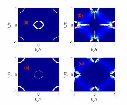
Figure 4: Plot of the integrand, $(\gamma_{\bf k}^{ll})^{2}({|\Delta_{\mathbf{k}}^{l}|/2\tilde{E}_{\mathbf{k}l}})^{2}$, in Eq. (13) in the first BZ. Frame (a)& (b) correspond respectively to $l=\alpha$ and $\beta$ with extended $s$-wave gap; frame (c)& (d) correspond respectively to $l=\alpha$ and $\beta$ with $d_{xy}$-wave gap.

We first consider the case of the extended $s$-wave pairing: $\Delta_{\bf k}^{l}=\Delta_{l}\cos(k_{x}/2)\cos(k_{y}/2)$ ($l=\alpha,\beta$) shown in Fig. 2(a). In a close observation of the $B_{2g}$ Raman spectra reported in Ref. PhysRevB.80.180510 , it is identified that only a single peak develops at $\omega=69$ cm^-1. This is an important point in terms of theoretical fitting. In our fitting, the key is thus to ensure that both bands give a peak at the same frequency ($\omega=69$ cm^-1). This one-peak scenario of fitting may seem unrealistic, but indeed it is the only way to successfully describe the presently available data. It is found that for the best fitting [see Fig. 3(a)], $\Delta_{\alpha}/\Delta_{\beta}=0.35$. The Raman peak occurs at $\omega/{2\Delta_{\beta}}=0.38$ which corresponds to gap magnitudes $\Delta_{\beta}=91$ cm^-1 and $\Delta_{\alpha}=32$ cm^-1. Moreover we have obtained $t_{1}=455$cm^-1.

In view of Fig. 3(a) for the best fitted curve, it is seen that $\beta$-band contributes most to the overall $B_{2g}$ Raman intensity. As mentioned before, $B_{2g}$ Raman vertex couples roughly equal to the $\alpha$ and $\beta$ bands, thus the individual contribution to the Raman intensity will depend crucially on the multiple effect of Raman vertex, symmetry and magnitude of the gap function, as well as the Fermi surface topology. To see this multiple effect, we have plotted in Fig. 4 the integrand, $(\gamma_{\bf k}^{ll})^{2}({|\Delta_{\mathbf{k}}^{l}|/2\tilde{E}_{\mathbf{k}l}})^{2}$, in Eq. (13) in the first BZ. It is shown that $\beta$-band has much stronger intensity near the $\beta$-band FS which results in a much stronger contribution to the overall Raman scattering [see Fig. 3(a)]. Moreover, due to the nature of an extended $s$-wave gap which has nodes at the BZ edges, Raman intensity is linear dependent at small frequencies.

The case of the $d_{xy}$-wave pairing in the unfolded BZ: $\Delta_{\bf k}^{l}=\Delta_{l}\sin(k_{x}/2)\sin(k_{y}/2)$ ($l=\alpha,\beta$) is studied next. As shown in Fig. 2(b), the gap amplitude in $\alpha_{2}$ FS is larger than that in $\alpha_{1}$ FS. Thus the Raman intensity due to the $\alpha$-band will mainly contributed by the $\alpha_{2}$-band FS. Due to the same gap amplitude near $\beta_{1}$ and $\beta_{2}$ FSs, they will contribute equally to the Raman intensity. In a similar approach, to obtain the same Raman peak for the two-band model, we again use the two-gap approach. It is found that $\Delta_{\alpha}/\Delta_{\beta}=0.3$ will give the best fitting for the experimental $B_{2g}$ data. Moreover the $B_{2g}$ Raman peak corresponds to $\omega/{2\Delta_{\beta}}=0.3$ which in turn gives $\Delta_{\beta}=115$ cm^-1, $\Delta_{\alpha}=34$ cm^-1, and $t_{1}=575$cm^-1. While $\alpha$ band FSs are fully gapped, $\beta$-band FSs are gapped with a node. Therefore the Raman intensity is powers-law dependent at low frequencies. Moreover, as $\beta$-band contributes most to the Raman intensity because of larger gap size, the low-energy $B_{2g}$ Raman intensity is actually linear.

The fitting to the Raman response in $B_{1g}$ channel is not feasible at the moment. There occurs a strong phonon mode at 214 cm^-1 due to the Fe vibration PhysRevB.80.180510 . The phonon mode is expected to be removed by changing the crystal structure slightly. We have calculated and predicted the $B_{1g}$ Raman responses for the extended $s$-wave pairing symmetry shown in Fig. 3(c) with the same parameters as those used in Fig. 3(a). As shown in Fig. 2(d), although $B_{1g}$ mode couples predominantly to the $\alpha$ band in XM directions, the gap amplitude of $\alpha$-band is smaller than that of the $\beta$-band. Consequently it results QP excitation from the two bands with the same weight approximately. The low-energy Raman response is predicted to be power-law dependent due to the full gap in both FSs.

We have also calculated and predicted the $B_{1g}$ Raman responses for the $d_{xy}$-wave pairing symmetry shown in Fig. 3(d) with the same parameters as those used in Fig. 3(b). As shown in Fig. 2(b), $\alpha_{1}$ FS is near gap node while $\alpha_{2}$ FS is fully gapped. Thus $\alpha_{1}$-band will contribute more to the low-energy Raman scattering than the $\alpha_{2}$-band. Since the gap amplitudes in $\beta_{1}$ FS is equal to that of $\beta_{2}$ FS, they have the same contribution to Raman scattering. Although the gap amplitude of $\alpha$-band is smaller than that of the $\beta$-band, $B_{1g}$ mode couples predominantly to the $\alpha$ band in XM directions however. It results that $\alpha$ bands contribute more to the Raman scattering than the $\beta$ band. The low-energy Raman response is predicted to be power-law dependent with frequency due to the full gap in $\alpha_{1}$ band FS.

Table 1: Summary of the fitting results for the three possible pairing symmetries on the $B_{2g}$ Raman intensity.PhysRevB.80.180510 Row 1 corresponds to the energy ratio of the $B_{2g}$ peak (occurs at 69cm^-1) to $2\Delta_{\beta}$. Row 2 and 3 are the gap amplitudes of $\Delta_{\beta}$ and $\Delta_{\alpha}$ in units of cm^-1 and row 4 are their ratios. Row 5 are the deduced values of $t_{1}$ in units of cm^-1.

Pairing Symmetry	extended $s$-wave	$d_{xy}$-wave	$d_{x^{2}-y^{2}}$-wave
${\omega}/{2\Delta_{\beta}}$	0.38	0.3	0.24
$\Delta_{\beta}$(cm-1)	91	115	143
$\Delta_{\alpha}$(cm-1)	32	34	14
$\Delta_{\alpha}/\Delta_{\beta}$	0.3	0.3	0.1
$t_{1}$(cm-1)	455	575	7150

To complete the studies, we have also studied the case of $d_{x^{2}-y^{2}}$-wave pairing symmetry. It is found that the best fitting of the $B_{2g}$ Raman intensity is given by the ratio $\Delta_{\alpha}/\Delta_{\beta}=0.1$ which in turn gives $t_{1}=7150$cm^-1. Based on the given unrealistically large $t_{1}$, we conclude that $d_{x^{2}-y^{2}}$-wave pairing is ruled out in terms of the current available Raman scattering data. Table 1 is a summary of the the fitting results for the $B_{2g}$ Raman intensity.

IV Summary

In summary, we have studied the Raman response of iron-pnictide superconductor in both normal and SC states based on a two-band model. Predictions are given for the normal-state Raman intensities. A more quantitative fitting to the currently available Raman spectra is made to which useful fitting parameters are quoted in terms of the gap amplitudes on both bands.

- (1) X. H. Chen et al., Nature 100, 247002 (2008)
- (2) X. C. Wang et al., Solid State Commun. 148, 538 (2008)
- (3) F.-C. Hsu et al., Proc. Nat. Acad. Sci. 105, 14262 (2008)
- (4) C. Liu et al., Phys. Rev. Lett. 101, 177005 (2008)
- (5) D. V. Evtushinsky et al., Phys. Rev. B 79, 054517 (2009)
- (6) A. Coldea et al., Phys. Rev. Lett. 101, 216402 (2008)
- (7) H. Ding et al., Europhys. Lett. 83, 47001 (2008)
- (8) L. Zhao et al., Chin. phys. Lett. 25, 4402 (2008)
- (9) I. I. Mazin, D. J. Singh, M. D. Johannes, and M. H. Du, Phys. Rev. Lett. 101, 057003 (2008)
- (10) F. Wang et al., Phys. Rev. Lett. 102, 047005 (2009)
- (11) C.-T. Chen et al., Nature Physics 6, 260 (2010)
- (12) S. Onari, H. Kontani, and M. Sato, Phys. Rev. B 81, 060504 (2010)
- (13) J. Zhao, L.-P. Regnault, C. Zhang, M. Wang, Z. Li, F. Zhou, Z. Zhao, C. Fang, J. Hu, and P. Dai, Phys. Rev. B 81, 180505 (2010)
- (14) C. W. Hicks et al., J. Phys. Soc. Jpn. 78, 013708 (2009)
- (15) K. Matano et al., Europhys. Lett. 83, 57001 (2008)
- (16) H.-J. Grafe et al., Phys. Rev. Lett. 101, 047003 (2008)
- (17) L. Shan et al., Europhys. Lett. 83, 57004 (2008)
- (18) T. Y. Chen et al., Nature 453, 1224 (2008)
- (19) T. P. Devereaux and R. Hackl, Rev. Mod. Phys. 79, 175 (2007)
- (20) B. Muschler, W. Prestel, R. Hackl, T. P. Devereaux, J. G. Analytis, J.-H. Chu, and I. R. Fisher, Phys. Rev. B 80, 180510 (2009)
- (21) G. R. Boyd, T. P. Devereaux, P. J. Hirschfeld, V. Mishra, and D. J. Scalapino, Phys. Rev. B 79, 174521 (2009)
- (22) A. V. Chubukov, I. Eremin, and M. M. Korshunov, Phys. Rev. B 79, 220501 (2009)
- (23) M. V. Klein, Physics 2, 46 (2009)
- (24) D. J. Singh and M.-H. Du, Phys. Rev. Lett. 100, 237003 (2008)
- (25) C. Cao, P. J. Hirschfeld, and H.-P. Cheng, Phys. Rev. B 77, 220506 (2008)
- (26) K. Kuroki, S. Onari, R. Arita, H. Usui, Y. Tanaka, H. Kontani, and H. Aoki, Phys. Rev. Lett. 101, 087004 (2008)
- (27) X. Dai, Z. Fang, Y. Zhou, and F.-C. Zhang, Phys. Rev. Lett. 101, 057008 (2008)
- (28) T. Li, Journal of Physics: Condensed Matter 20, 425203 (2008)
- (29) S. Raghu, X.-L. Qi, C.-X. Liu, D. J. Scalapino, , and S.-C. Zhang, Phys. Rev. B 77, 220503(R) (2008)
- (30) G. Xu, W. Ming, Y. Yao, X. Dai, S.-C. Zhang, and Z. Fang, EPL 82, 67002 (2008)
- (31) T. P. Devereaux and D. Einzel, Phys. Rev. B 51, 16336 (1995)
- (32) J. Linder and A. Sudbø, Phys. Rev. B 79, 020501 (2009)
- (33) Z. Nazario and D. I. Santiago, Phys. Rev. B 70, 144513 (2004)
- (34) When the pairing symmetry in the unfolded BZ is extended -wave with [see Fig. 2(a)], it will transform to be in the folded BZ. Similarly, when the pairing symmetry in the unfolded BZ is extended -wave with [see Fig. 2(b)], it will transform to be in the folded BZ.