Topologically Protected Zero Modes in Twisted Bilayer Graphene

Abstract

We show that the twisted graphene bilayer can reveal unusual topological properties at low energies, as a consequence of a Dirac-point splitting. These features rely on a symmetry analysis of the electron hopping between the two layers of graphene and we derive a simplified effective low-energy Hamiltonian which captures the essential topological properties of twisted bilayer graphene. The corresponding Landau levels peculiarly reveal a degenerate zero-energy mode which cannot be lifted by strong magnetic fields.

I Introduction

One of the most fascinating aspects of graphene is its band structure which can be fundamentally changed in several different ways by modifying its lattice structure. This happens because the honeycomb lattice of monolayer graphene has two independent sublattices and the electron, as it moves through the lattice, has to change its sublattice and hence the character of its wavefunction.Revs Thus, even small local changes in the lattice structure lead to the appearance of gauge potentials which are associated with the phase of the electronic wavefunction in each sublattice. As a consequence, there is a one-to-one correspondence between graphene’s structure with the topological features of the electronic states.

Another amazing property of graphene is its honeycomb structure which yields an electronic low-energy effective theory which is Lorentz-invariant in two dimensions (2D), and thus corresponds to 2D Dirac fermions. This Lorentz invariance is robust because the energy associated with sublattice coupling, that is, the inter-sublattice hopping energy $t$ ($\approx 3$ eV) is the dominant energy scale in the system. Lorentz invariance persists even when the lattice is modified either by external forces (strain, shear, etc.),strain by external fields, or by the addition of more layers.Lorentz For instance, AB-stacked bilayer graphene is described, at low energies by two sets of massive Lorentz invariant Dirac particles per valley and spin. In the simplest models where only nearest neighbor hoppings are taking into account, there is still an accidental degeneracy that makes the particle-like band of one flavor to be degenerate with the anti-particle-like (hole-like) band of the other flavor at the K (K’) point in each valley. This degeneracy can be easily lifted by the application of a perpendicular electric field that breaks the inversion symmetry in the system.Revs Although the Lorentz invariance is preserved, the wavefunction of the electrons at low energies is modified$-$whereas in monolayer graphene the Dirac fermions carry a Berry phase $\pm\pi$, the Berry phase is $\pm 2\pi$ in AB-stacked bilayer graphene.MF06 At low energies, trigonal warping splits this “double” Dirac point into three with a Berry phase $\pi$ and an additional one with $-\pi$,MF06 a situation that persists for a translational mismatch between the layers.Son

Twisted bilayer graphene, in which the two layers have a rotational mismatch described by an angle $\theta$ as compared to the perfect AB stacking, is another example where lattice structure and wavefunction topology are directly interconnected. In fact, from the experimental point of view, twisted graphene is more the rule than the exception. It naturally occurs at the surface of graphite,Rong ; Pong in graphene grown in the surface of SiC,Hass or graphene grown by chemical vapor deposition on metal substrates.Eva As compared to monolayer graphene, each Dirac flavor is then split into two copies that are separated in reciprocal space by a wave vector $\Delta{\bf K}$, as a function of $\theta$.Lopes Inter-layer hopping results in a renormalization of the Fermi velocityHeer ; Schmidt ; Lopes ; Shallcross as well as in a van Hove singularity at relatively low energy as compared to that in monolayer graphene.Lopes ; Eva Once again, Lorentz invariance is preserved at low energies but the nature of the electronic wavefunctions is modified in a profound way.

In this paper, we investigate the topological aspects of the band structure of twisted graphene bilayers at low energies in the continuum approximation, for small angle mismatches as compared to perfect AB stacking. We identify possible topological classes that describe band inversion symmetry. These topological classes determine the relative Berry phase between the two copies of Dirac particles, which have either the same or opposite Berry phase. If the two Dirac cones are related by time-reversal symmetry, such as the $K$ and $K^{\prime}$ points in monolayer graphene, the Berry phases are naturally opposite. In twisted graphene bilayers, however, the two Dirac points emanating from different layers are not time-related, and the symmetry of the inter-layer hopping term enforces the Berry phases to be identical. We show that this feature yields a topologically protected zero-energy Landau level, in contrast to the former case. The scenario may be tested in quantum Hall measurements.

The paper is organized as follows. In Sec. II, we discuss the model of twisted bilayer graphene and the symmetry properties of their bands (Sec. II.1) that are fixed by the form of the inter-layer hopping. Furthermore, we present an effective two-band model (Sec. II.2) that displays the same topological low-energy properties as the original four-band model. Section III is devoted to the discussion of the Landau-level spectrum in twisted bilayer graphene, in the perspective of possible quantum-Hall measurements.

Figure 1: First Brillouin zone for twisted bilayer graphene. The 1BZ of the upper layer (dashed hexagon) is rotated by an angle $\theta$ with respect to that of the lower layer (full hexagon). The corners, where Dirac points occur, are labeled by $K_{\theta}^{(\prime)}$ and $K^{(\prime)}$, respectively.

II Model of twisted bilayer graphene

If we neglect, for the moment, hopping between atoms in different layers, the electronic properties of twisted bilayer graphene are described by two copies of the Hamiltonian for monolayer graphene (we use units with $\hbar=1$):

$$H_{0}({\bf k})\equiv v_{F}\left(\begin{array}[]{cc}0&k^{*}\\ k&0\end{array}\right),$$ (1)

where $v_{F}$ is the Fermi velocity and $k=k_{x}+ik_{y}$ is the 2D wave-vector relative to the K (K’) points of the rotated layers (see Fig.1). For a twist (rotation) angle $\theta\neq 0$, each of the two inequivalent Dirac points, which reside at the corners of the first BZ $K$ and $K^{\prime}$, are split into two, separated by a wave vector $\Delta{\bf K}={\bf K}-{\bf K}_{\theta}$, where ${\bf K}_{(\theta)}$ is the position of the $K$ point in the lower (upper) layer and $-{\bf K}_{(\theta)}$ the position of the points $K^{\prime}$ and $K_{\theta}^{\prime}$, respectively. Throughout this paper, we will work in the continuum limit around a single pair ($K$,$K_{\theta}$) and, therefore, neglect commensuration effects between the two layers which could enlarge the unit cell in position space and thus fold it back in reciprocal space. This procedure is mostly justified because the coupling between the pairs of Dirac conesMele ; MacDonald is negligible.Shallcross

The Hamiltonian describing the electronic properties of twisted bilayer graphene reads

$$H({\bf k})=\left(\begin{array}[]{cc}H_{0}({\bf k}+\Delta{\bf K}/2)&H_{\perp}\\ H_{\perp}^{\dagger}&H_{0}({\bf k}-\Delta{\bf K}/2)\end{array}\right),$$ (2)

where $H_{\perp}$ is the hopping matrix between the two layers. Equation (2) refers to an expansion around the ${\bf Q}$ point of Fig. 1. The analysis of the Moiré pattern formed by the twisted bilayer shows that, for small angle $\theta$, the hopping matrix $H_{\perp}$ may have three different forms corresponding to the three main Fourier components.Lopes ; MacDonald This leads to three different types of inter-layer hopping terms,

$$H_{\perp}^{0}\equiv\tilde{t}_{\perp}\left(\begin{array}[]{cc}1&1\\ 1&1\\ \end{array}\right),\quad H_{\perp}^{\pm}\equiv\tilde{t}_{\perp}\left(\begin{array}[]{cc}e^{\mp i\phi}&1\\ e^{\pm i\phi}&e^{\mp i\phi}\\ \end{array}\right),$$ (3)

where $\phi=2\pi/3$ and $\tilde{t}_{\perp}$ is a hopping parameter which generally depends on $\theta$.Lopes ; MacDonald ; note

II.1 Symmetry of the bands and Berry phases

In contrast to a lattice Hamiltonian that may be analyzed with the help of global symmetries, such as time reversal or lattice inversion, $H({\bf k})$ in Eq. (2) is a continuum model in which the two Dirac points are no longer related by these symmetries. However, $H({\bf k})$ and the inter-layer hopping term $H_{\perp}$ may be investigated via symmetries that involve directly the energy bands, such as rotation, mirror, and inversion symmetry. Whereas for $H_{\perp}=0$ the rotation and inversion symmetries are respected, the latter are broken for non-zero inter-layer hopping, and we therefore restrict the discussion to the inversion symmetry $\mathcal{I}$ of the bands. We emphasize that this inversion symmetry is defined with respect to the bands in reciprocal space, in contrast to a previous analysis,Paco in which the more common definition of inversion symmetry with respect to the lattice was used.

In the absence of any inter-layer hopping, the Hamiltonian (2) would be ambiguous since one could work equally well with $H_{0}^{*}$ in the second layer. As a consequence, there remain two possible representations of inversion (with different spinorial expressions) $\mathcal{I}_{1}$ and $\mathcal{I}_{2}$:

$$\mathcal{I}_{1}:H(-{\bf k})=-H({\bf k})\qquad{\rm or}\qquad\mathcal{I}_{2}:H(-{\bf k})=-H({\bf k})^{*}.$$ (4)

The minus signs in both transformations maps positive to negative energy states at opposite wave vectors and vice-versa: $E({\bf k})\rightarrow-E(-{\bf k})$, whereas the complex conjugation in $\mathcal{I}_{2}$ changes the relative phase between the spinor components and, hence, the Berry phase of a cone.

The phases of the two Dirac points are thus different for the two representations. For the $\mathcal{I}_{1}$ case, the Berry phases at fixed energy are opposite such that a merging transition of the two Dirac points (at $\theta=0$) corresponds to a vanishing total Berry phase and consequently to the possible opening of a band gap. This situation arises e.g. in the framework of the model discussed in Refs. listDPmerg, , which describes monolayer graphene under strong strain.strain In contrast to this rather well-known topological universality class, the transformation $\mathcal{I}_{2}$ yields Berry phases that are the same at fixed energy $E$ and opposite to those at $-E$ and thus represents a second universality class for Hamiltonians describing pairs of Dirac points. The transformation $\mathcal{I}_{2}$ may be represented in terms of a tensor product of Pauli matrices, $\mathcal{I}_{2}=\sigma_{y}^{E}\otimes\sigma_{x}^{A}$, where $\sigma_{x/y}^{A}$ and $\sigma_{x/y}^{E}$ describe the intra-layer and the inter-layer spinorial spaces, respectively. The phases are eventually fixed by the symmetry of the interlayer hopping $H_{\perp}$, and the particular forms (3) happen to be invariant under $\mathcal{I}_{2}$.

Notice, however, that as a consequence of the inter-layer hopping terms (3), the two Dirac points are no longer exactly at the same energy, but we neglect this energy shift here because it is associated with a very small energy scale $\sim 1$ meV. As a second-order perturbation, this indeed scales like $\tilde{t}_{\perp}^{2}/(v_{F}\Delta{\bf K})$ with $\tilde{t}_{\perp}$ of the order of $100$ meV and $v_{F}\Delta{\bf K}\sim 1$ eV.Lopes

II.2 Effective two-band model

In the opposite limit, $\tilde{t}_{\perp}\gg v_{F}\Delta K$, the model (2) may be reduced to an effective two-band model, similarly to the case of a perfectly AB-stacked ($\theta=0$) graphene bilayer.MF06 This is done in two steps. First, one replaces $H_{\perp}$ in Eq. (2) by a simplified inter-layer hopping term,

$$H_{\perp}^{\rm eff}=\tilde{t}_{\perp}\left(\begin{array}[]{cc}0&0\\ 1&0\end{array}\right),$$ (5)

in the limit where $\tilde{t}_{\perp}\gg v_{F}\Delta K$, i.e. for small tilt angles. The inter-layer hopping term (5) is reminiscent of the Bernal bilayer case. In spite of this simplification and the difference in the energy scales, the resulting Hamiltonian may be viewed as a representative of the topological universality class that also includes the original four-band model. We consider the eigenvectors of Eq. (5) in terms of the 4-spinor basis $\left\{\psi_{A},\psi_{B},\psi_{A^{\prime}},\psi_{B^{\prime}}\right\}$ where $(A,B)$ belongs to the two sublattices of the first layer and $(A^{\prime},B^{\prime})$ to that of the second one. With the particular form of Eq. (5), the zero-energy sector is spanned $\psi_{A}$ and $\psi_{B^{\prime}}$, whereas $\psi_{B}$ and $\psi_{A^{\prime}}$ are strongly hybridized by the inter-layer hopping term. Their symmetric and anti-symmetric combinations are the eigenstates at $-\tilde{t}_{\perp}$ and $\tilde{t}_{\perp}$, respectively. In order to describe the electronic properties in the vicinity of $E=0$, one may therefore project the Hamiltonian onto the reduced $\left\{\psi_{A},\psi_{B^{\prime}}\right\}$ basis and neglecting terms of the form $E\psi_{B/A^{\prime}}$, which are a product of the energy $E\sim 0$ and the small components $\psi_{B/A^{\prime}}$. The eigenvalue problem reads

$$v_{F}(k+\Delta K/2)^{*}\psi_{B} = E\psi_{A}$$ (6)

$$v_{F}(k+\Delta K/2)\psi_{A}+\tilde{t}_{\perp}\psi_{A^{\prime}} = E\psi_{B}\simeq 0$$ (7)

$$\tilde{t}_{\perp}\psi_{B}+v_{F}(k-\Delta K/2)^{*}\psi_{B^{\prime}} = E\psi_{A^{\prime}}\simeq 0$$ (8)

$$v_{F}(k-\Delta K/2)\psi_{A^{\prime}} = E\psi_{B^{\prime}}.$$ (9)

By rewriting Eqs. (8) and (9),

$$-v_{F}/\tilde{t}_{\perp}(k+\Delta K/2)\psi_{A} = \psi_{A^{\prime}}$$ (10)

$$-v_{F}/\tilde{t}_{\perp}(k-\Delta K/2)^{*}\psi_{B^{\prime}} = \psi_{B},$$ (11)

and substituting them into Eqs. (6) and (9), one obtains the Schrödinger equation

$$H^{\text{eff}}({\bf k})\left(\begin{array}[]{c}\psi_{A}\\ \psi_{B^{\prime}}\end{array}\right)=E\left(\begin{array}[]{c}\psi_{A}\\ \psi_{B^{\prime}}\end{array}\right),$$ (12)

in terms of the effective two-band Hamiltonian

$$H^{\text{eff}}({\bf k})=-\frac{v_{F}^{2}}{\tilde{t}_{\perp}}\left(\begin{array}[]{cc}0&\left(k^{*}\right)^{2}-\left(\Delta K^{*}\right/2)^{2}\\ k^{2}-\left(\Delta K/2\right)^{2}&0\\ \end{array}\right),$$ (13)

which is similar to that for the nematic transition of the interacting Bernal graphene bilayer.Vafek

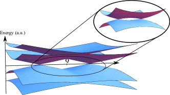
Figure 2: (Color online) Generic band structure for the lowest four bands of the twisted bilayer graphene, around the ${\bf Q}$ point, with only $H_{\perp}^{0}$ considered. The inset of the figure pictures the effective bands of the model Hamiltonian (13). Both band structures are inversion-invariant with respect to the ${\bf Q}$ point.

The generic form of the band structure obtained from the effective two-band model (13) is depicted in the inset of Fig. 2. One notices the two Dirac points originally situated at ${\bf K}$ and ${\bf K}_{\theta}$, separated by a wave vector $|\Delta{\bf K}|\sim\theta/a$ in the first BZ, in terms of the intra-layer distance $a=0.142$ nm between neighboring carbon atoms. In order to see the linearity of the dispersion relation in the vicinity of these contact points, one can further expand the Hamiltonian (5) around $\pm\Delta{\bf K}/2$, by defining ${\bf k}={\bf q}\pm\Delta{\bf K}/2$, with $|{\bf q}|\ll|\Delta{\bf K}|/2$. This expansion yields two Dirac Hamiltonians

$$\pm\frac{v_{F}^{2}\Delta K}{\tilde{t}_{\perp}}\left(\begin{array}[]{cc}0&q^{*}\\ q&0\end{array}\right),$$ (14)

with identical chirality for the two contact points.

Furthermore, the bands have saddle points at ${\bf k}=0$ between the two Dirac points. The effective two-band Hamiltonian therefore captures the logarithmic van-Hove singularity in agreement with previous theoreticalLopes and experimental studies.Li10

The most salient features of the Hamiltonian (13) are its chiral properties. In agreement with the above-mentioned general symmetry considerations, electrons at a fixed energy at the ${\bf K}$-point have the same chirality as those at the ${\bf K}_{\theta}$ point, such that in both cases the electron experiences the same Berry phase $\gamma=\pi$ (and $\gamma=-\pi$ at the points ${\bf K}^{\prime}$ and ${\bf K}_{\theta}^{\prime}$) on a closed orbit around one of the Dirac points. This is obvious in the low-energy expansion (14) around the two Dirac points. As for AB-stacked bilayer graphene, the Berry phase acquired on an orbit enclosing both Dirac points is then $2\gamma$, as one may also see from the limit of vanishing twist angle ($\theta=0$) which reproduces the perfectly AB-stacked bilayer.MF06 Furthermore, it becomes apparent from the form of the Hamiltonian (13) that the merging of the Dirac points is not accompanied with a gap opening, in contrast to the Hamiltonian discussed in Ref. listDPmerg, , which desribes the same band structure in the semi-metallic phase but which belongs to another topological class, described by the symmetry $\mathcal{I}_{1}$.

III Landau levels of twisted bilayer graphene

One of the most prominent consequences of these topological properties is the presence of a (doubly-degenerate) zero mode that emerges in the presence of a quantizing magnetic field, in which case the Hamiltonian (13) may be written in terms of the usual ladder operators $a$ and $a^{\dagger}$, with $[a,a^{\dagger}]=1$:

$$H_{B}=\omega_{C}\left(\begin{array}[]{cc}0&a^{2}-\alpha^{*2}\\ a^{\dagger 2}-\alpha^{2}&0\end{array}\right),$$ (15)

where $\omega_{C}=2v_{F}^{2}eB/\tilde{t}_{\perp}$ is the cyclotron frequency and $\alpha\equiv\Delta Kl_{B}/2\sqrt{2}$. As compared to the perfectly AB-stacked bilayer ($\alpha=0$), where one readily obtains the Landau level (LL) spectrum,MF06 one notices that the additional terms couple states only of the same parity. One obtains thus two classes of eigenstates $\psi_{2n}$ and $\psi_{2n+1}$ that may be written in the usual harmonic-oscillator basis $|m\rangle$, with $a^{\dagger}a|m\rangle=m|m\rangle$:

$$\Psi_{2n(+1)}=\sum_{m=0}^{\infty}\left(\begin{array}[]{c}\phi_{2m(+1)}^{1}\\ \phi_{2m(+1)}^{2}\end{array}\right)|2m(+1)\rangle,$$ (16)

where the components $\phi_{m}^{1}$ and $\phi_{m}^{2}$ are to be determined recursively.

III.1 Zero-energy levels

Before discussing the LL spectrum of Hamiltonian (15), we investigate the zero-energy states, which may be obtained analytically from the equation $H_{B}\Psi=0$. As for the AB-stacked bilayer, one obtains two distinct solutions, one with even and one with odd parity, such that the zero-energy level is orbitally two-fold degenerate, in addition to its usual four-fold spin-valley degeneracy and the orbital degeneracy described by the flux density $n_{B}=eB/h$. The two zero-energy states, which are reminiscent of coherent states, are directly obtained from the secular equation:

$$\Psi_{0} = \mathcal{N}_{0}\cosh(\alpha^{*}a^{\dagger})\left(\begin{array}[]{c}0\\ |n=0\rangle\end{array}\right),$$ (19)

$${\rm and}\qquad\Psi_{1} = \mathcal{N}_{1}\frac{\sinh(\alpha^{*}a^{\dagger})}{\alpha^{*}}\left(\begin{array}[]{c}0\\ |n=0\rangle\end{array}\right),$$ (22)

in terms of the normalization factors $\mathcal{N}_{0/1}$. These states are generalizations of the zero-energy states $(0,|0\rangle)$ and $(0,|1\rangle)$ of the AB-stacked bilayer.MF06 . We also notice that we neglect any other potential lifts due to Zeeman effect and/or interactions.goerbig10

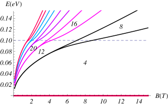
Figure 3: (Color online) Landau levels of twisted bilayer graphene, obtained from the numerical solution of Eq. (15). The characteristic energy scale of the van-Hove singularity has been chosen as $|\alpha|^{2}\omega_{C}=(\Delta K)^{2}/8m=0.1$eV. The red line indicates the zero-energy level, and the numbers correspond to the filling factors in the gaps.

The existence of those zero-mode states is independent of the strength of the magnetic field. This is to be compared to the other topological class of Dirac cones with opposite Berry phases where the degeneracy of the zero-mode is lifted.listDPmerg This protection is solely determined by the topology of the model Hamiltonian since the band-structures are otherwise identical. Notice further that the scaling of the Landau levels relative to $\Delta{\bf K}$ is different for the two topological classes.

III.2 Full Landau-level spectrum

The full LL spectrum, which has been calculated numerically, is depicted in Fig. 3. In the regime of small magnetic fields, the LLs with small index $n\ll n_{C}$, where $n_{C}$ denotes roughly the LL which crosses the van-Hove singularity, $\sqrt{n_{C}B}\sim v_{F}|\Delta K|^{2}/4\sqrt{2}\tilde{t}_{\perp}$, display the $\sqrt{Bn}$ behavior, which is the benchmark of massless Dirac fermions, as expected for the linear dispersion below the van-Hove singularity. Because of the two Dirac points, these LLs, as well as the zero-energy level discussed above, are twofold degenerate, in addition to the fourfold spin-valley degeneracy. The twofold degeneracy due to the Dirac-point splitting in the twisted bilayer is lifted once the LLs approach and eventually cross the van-Hove singularity, $n\gtrsim n_{C}$, above which the LLs scale as $\sim B(n+1/2)$, as one would expect from the parabolic dispersion relation revealed by Hamiltonian (13) at high energies. Notice, however, that as for AB-stacked bilayer graphene the effective two-band approximation is no longer valid at higher energies (far beyond the van-Hove singularity) because of the presence of the remaining bands, which become visible there.

The LL spectrum in Fig. 3 allows one to understand the main features of a quantum Hall effect (QHE) in twisted bilayer graphene. The topologically protected zero-energy LL, with its altogether eightfold degeneracy, yields a QHE at filling factors $\nu=\pm 4$ (taking into account spin degeneracy). This feature is independent of the interlayer hopping strength $t_{\perp}$ and of the van-Hove singularity, which is triggered by the twist angle $\theta$. For other LLs, the position of the van-Hove singularity determines their degeneracy. If the LLs remain well below the singularity, $n\ll n_{C}$, they maintain their eightfold degeneracy, and one would therefore expect Hall plateaus at filling factors $\nu=\pm 4(2n+1)=\pm 4,\pm 12,\pm 20,...$, but one would expect additional plateaus at $\nu=\pm 8,\pm 16,...$ for LLs with $n\gtrsim n_{C}$. The experimentLee10 indicates, even at rather low magnetic fields of $B\sim 5$T, only the zero-energy LL is eightfold degenerate, whereas a plateau at $\nu=\pm 8$ has been observed. This stipulates that the energy of the van-Hove singularity is as small as the first excited LL.

IV Conclusions

In conclusion, we have investigated the topological band structure of twisted bilayer graphene, in the framework of a symmetry analysis of the inter-layer hopping in the continuum limit. For small and moderate twist angles $\theta$, the two copies of the Dirac point (that are not related by time-reversal symmetry) are described by the same Berry phase, due to the the symmetry of the inter-layer hopping term. Therefore, they belong to a different topological class than the (usual) two Dirac points, which are related by time-reversal symmetry. In the presence of a quantizing magnetic field, these particular topological properties yield a protected zero-energy LL with an eight-fold degeneracy that may be evidenced in quantum Hall transport measurements.

- (1) For a review, see A. H. Castro Neto, F. Guinea, N. M. R. Peres, K. S. Novoselov, and A. K. Geim, Rev. Mod. Phys. 81, 109 (2009).
- (2) C. Lee, X. Wei, J. K. Kysar, and J. Hone, Science 321, 385 (2008); M. O. Goerbig, J.-N. Fuchs, G. Montambaux, and F. Piéchon, Phys. Rev. B 78, 045415 (2008); V. M. Pereira, A. H. Castro Neto, and N. M. R. Peres, Phys. Rev. B 80, 045401 (2009).
- (3) B. Partoens and F. M. Peeters, Phys. Rev. B 75, 193402 (2007); M. Koshino and T. Ando, ibid. 76, 085425 (2007); S. Latil, V. Meunier, and L. Henrard, Phys. Rev. B 76, 201402 (2007); J. Nilsson, A. H. Castro Neto, F. Guinea, and N. M. R. Peres, ibid. 78, 045405 (2008).
- (4) E. McCann and V. I. Fal’ko, Phys. Rev. Lett. 96, 086805 (2006)
- (5) Y.-W. Son, S.-M. Choi, Y. P. Hong, S. Woo and S.-H. Jhi, preprint arXiv:1012.0643.
- (6) Z. Y. Rong and P. Kuiper, Phys. Rev. B 48, 17427 (1993).
- (7) W. T. Pong and C. Durkan, J. Phys. D 38, R329 (2005).
- (8) J. Hass, F. Varchon, J. E. Millán-Otoya, M. Sprinkle, N. Sharma, W. A. de Heer, C. Berger, P. N. First L. Magaud, and E. H. Conrad, Phys. Rev. Lett. 100, 125504 (2008).
- (9) A. Luican, G. Li, A. Reina, J. Kong, R. R. Nair, K. S. Novoselov, A. K. Geim, and E. Y. Andrei, Phys. Rev. Lett. 106, 126802 (2011).
- (10) J. M. B. Lopes dos Santos, N. M. R. Peres, and A. H. Castro Neto, Phys. Rev. Lett. 99, 256802 (2007).
- (11) S. Shallcross, S. Sharma, and O. A. Pankratov, Phys. Rev. Lett. 101, 056803 (2008); S. Shallcross, S. Sharma, E. Kandelaki, and O. A. Pankratov, Phys. Rev. B 81, 165105 (2010).
- (12) H. Schmidt, T. Lüdtke, P. Barthold, and R. J. Haug, Phys. Rev. B 81, 121403.
- (13) W. A. de Heer, C. Berger, X. Wu, P. N. First, E. H. Conrad, X. B. Li, T. B. Li, M. Sprinkle, J. Hass, M. Sadowski, M. Potemski, and G. Martinez, Solid State Comm. 143, 92 (2007).
- (14) E. J. Mele, Phys. Rev. B 81, 161405(R) (2010),
- (15) R. Bistritzer and A. H. MacDonald, Phys. Rev. B 81, 245412 (2010); arXiv:1009.4203 (2010); arXiv:1101.2606 (2011).
- (16) The Hamiltonian (2) is similar to that of Ref. MacDonald, up to a low-angle expansion.
- (17) J. L. Mañes, F. Guinea, and M. A. H. Vozmediano, Phys. Rev. B 75, 155424 (2007).
- (18) P. Dietl, F. Piéchon, and G. Montambaux, Phys. Rev. Lett. 100, 236405 (2008); B. Wunsch , New J. Phys. 10, 103027 (2008); G. Montambaux, G., F. Piéchon, J.-N. Fuchs, and M. O. Goerbig, Phys. Rev. B 80, 153412 (2009); Eur. Phys. J. B 72, 509 (2009).
- (19) O. Vafek and K. Yang, Phys. Rev. B 81, 041401(R) (2010).
- (20) G. Li, A. Luican, J. M. B. Lopes dos Santos, A. H. Castro Neto, A. Reina, J. Kong, E.Y. Andrei, Nature Physics 6, 109 (2010).
- (21) M. O. Goerbig, to be published in Rev. Mod. Phys., arXiv:1004.3396.
- (22) D. S. Lee, C. Riedl, T. Beringer, K. v. Klitzing, U. Stake, and J. H. Smet, unpublished