Elemental abundances of low-mass stars in the young clusters 25 Ori and $\lambda$ Ori

Abstract

Aims. We aim to derive the chemical pattern of the young clusters 25 Orionis and $\lambda$ Orionis through homogeneous and accurate measurements of elemental abundances.

Methods. We present flames/uves observations of a sample of 14 K-type targets in the 25 Ori and $\lambda$ Ori clusters; we measure their radial velocities, in order to confirm cluster membership. We derive stellar parameters and abundances of Fe, Na, Al, Si, Ca, Ti, and Ni using the code MOOG.

Results. All the 25 Ori stars are confirmed cluster members without evidence of binarity; in $\lambda$ Ori we identify one non-member and one candidate single-lined binary star. We find an average metallicity [Fe/H]=$-0.05\pm 0.05$ for 25 Ori, where the error is the $1\sigma$ standard deviation from the average. $\lambda$ Ori members have a mean iron abundance value of $0.01\pm 0.01$. The other elements show close-to-solar ratios and no star-to-star dispersion.

Conclusions. Our results, along with previous metallicity determinations in the Orion complex, evidence a small but detectable dispersion in the [Fe/H] distribution of the complex. This appears to be compatible with large-scale star formation episodes and initial non-uniformity in the pre-cloud medium. We show that, as expected, the abundance distribution of star forming regions is consistent with the chemical pattern of the Galactic thin disk.

1 Introduction

In the last ten years, several studies have focused on the determination of the chemical composition of open clusters with ages $\raisebox{-2.15277pt}{$\>\stackrel{{\scriptstyle\textstyle>}}{{\sim}}\>$}100$ Myr; less attention has been paid to abundances of $\sim 10-100$ Myr old clusters (D’Orazi & Randich 2009, and references therein), and to the chemical pattern of young ($\raisebox{-2.15277pt}{$\>\stackrel{{\scriptstyle\textstyle<}}{{\sim}}\>$}10$ Myr) clusters and star forming regions (hereafter, SFRs; James et al. 2006; Santos et al. 2008; Biazzo et al. 2011, and references therein). Instead, elemental abundances of very young clusters and SFRs provide a powerful tool to investigate the possible common origin of different subgroups, to investigate scenarios of triggered star formation, and to trace the chemical composition of the solar neighborhood and Galactic thin disk at recent times.

Also, whilst the correlation between stellar metallicity and the presence of giant planets around old solar-type stars is well established (Gonzalez 1998; Santos et al. 2001; Johnson et al. 2010) and seems to be primordial (Gilli et al. 2006), the presence of a metallicity-planet connection at early stages of planet formation is still a matter of debate. On the one hand, the efficiency of dispersal of circumstellar (or proto-planetary) disks, the planet birthplace, is predicted to depend on metallicity (Ercolano & Clarke 2010). In a recent study, Yasui et al. (2010) find that the disk fraction in significantly low-metallicity clusters ([O/H]$\sim-0.7$) declines rapidly in $<1$ Myr, which is much faster than the value of $\sim 5-7$ Myr observed in solar-metallicity clusters. They suggest that, since the shorter disk lifetime reduces the time available for planet formation, this could be one of the reasons for the strong planet-metallicity correlation. On the other hand, Cusano et al. (2011) find that a significant fraction of the oldest pre-main sequence stars in the SFR Sh 2-284 have preserved their accretion discs/envelopes, despite the low-metallicity environment. Moreover, none of the SFRs with available metallicity determination is metal rich, challenging a full understanding of the metallicity-planet connection at young ages. Additional measurements of [Fe/H] in several star forming regions and young clusters are thus warranted.

In a recent paper, we have presented an homogeneous determination of the abundance pattern in the Orion Nebula Cluster (ONC) and the OB1b subgroup (Biazzo et al. 2011). We report here an abundance study of two other young groups belonging to the Orion complex; namely, the 25 Orionis and $\lambda$ Orionis clusters. Although the two clusters have been extensively observed and analyzed, no abundance measurement is available for 25 Ori, while for $\lambda$ Ori the metallicity of only one member has been derived (namely, Dolan 24; D’Orazi et al. 2009). The metallicity of these two clusters will allow us to put further constrains on the metal distribution in the whole Orion complex; furthermore, the age of 25 Ori ($\sim 7-10$ Myr; Briceño et al. 2005) and $\lambda$ Ori ($\sim 5-10$ Myr; Dolan & Mathieu 2002) is comparable to the maximum lifetime of accretion disks as derived from near-IR studies and can be considered indicative of the timescale for the formation of giant planets. For these reasons, measurements of [Fe/H] and other elements in such clusters are important and timely.

The 25 Ori group is a concentration of T Tauri stars (TTS) in the Orion OB1a subassociation, roughly surrounding the B2e star 25 Ori; this stellar aggregate was first recognized by Briceño et al. (2005) during the course of the CIDA Variability Survey of Orion (CVSO) as a distinct feature centered at $\alpha_{\rm J2000.0}=$5^h23^m and $\delta_{\rm J2000.0}=$1^°45^′. The 25 Orionis group was also reported by Kharchenko et al. (2005) as ASCC-16 in their list of 109 new open clusters identified through parallaxes, proper motions, and photometric data. Briceño et al. (2007) determined radial velocities of the cluster candidates, finding that the 25 Ori group constitutes a distinct kinematic group from the other Orion subassociations. The color-magnitude diagram, the lithium equivalent widths, and the fraction of CTTS ($\sim$6%) are consistent with the 25 Ori group being older than Ori OB1b (age $\sim 4-5$ Myr; Briceño et al. 2007). Finally, the same authors derive a cluster radius of $\sim 7$ pc centered 23.6^′ southeast of the star 25 Ori, with some indication of extension farther north.

The $\lambda$ Orionis cluster, discovered by Gomez & Lada (1998), is distributed over an area of 1 square degree around the O8 III star $\lambda^{1}$ Ori (at a distance of 400 pc; Murdin & Penston 1977). As suggested by Dolan & Mathieu (1999, 2001), the star formation process in this region began some 8–10 Myr ago in the central region and has since been accelerating, followed by an abrupt decline $\sim$1–2 Myr ago due to a supernova (SN) explosion (Cunha & Smith 1996). CO surveys clearly show that the central region of the cluster, composed by eleven OB stars, has been largely vacated of molecular gas. A ring of neutral and molecular hydrogen with a diameter of $\sim$9° surrounds an H ii region, and is likely the consequence of the sweeping of interstellar gas by the H ii region (see, e.g., Lang et al. 2000, and references therein).

In Sect. 2 we describe the target selection, observations, and data reduction. In Sect. 3 the radial velocity and elemental abundance measurements are determined, while the discussion and conclusions are presented in Sect. 4 and 5.

2 Observations and data analysis

2.1 Target selection

We selected four K2-K7 members of 25 Ori from the Briceño et al. (2007) sample, and four additional stars located about 1 degree to the north-east (Briceño et al. 2011, in preparation). These four targets, candidate pre-main sequence (PMS) stars in the CVSO dataset, were included for follow-up observations with the Hectospec and Hectochelle spectrographs at the 6.5m MMT (Arizona), in order to investigate the extent of the 25 Ori aggregate. As for $\lambda$ Ori, we selected four stars from the Dolan & Mathieu (1999) sample and two candidates from Barrado et al. (2004).

The distribution in the sky of the sample stars is shown in Figs. 1 and 2 overlaid on CO maps. Both samples lie away from giant molecular clouds and dark clouds, i.e. far from regions where star formation is actively occurring.

In Table 1 we list the sample stars along with information from the literature. In particular, in Columns 1–5 we give for the 25 Ori stars the name, $VJK$ magnitude, spectral type, and object class from Cutri et al. (2003), and Briceño et al. (2005; 2007; 2011, in preparation), while for the $\lambda$ Ori stars the name, $VJK$ magnitude, spectral type, and disk property are from Dolan & Mathieu (1999), Cutri et al. (2003), Zacharias et al. (2004), Sacco et al. (2008), and Hernández et al. (2010). In the last Column of both samples, radial velocities from Dolan & Mathieu (1999), Briceño et al. (2007), and Sacco et al. (2008) are given.

Both samples were selected with the following criteria: $i)$ no evidence of extremely high accretion; $ii)$ no evidence of high rotational velocity ($v\sin i\raisebox{-2.15277pt}{$\>\stackrel{{\scriptstyle\textstyle>}}{{\sim}}\>$}30$ km/s), and $iii)$ no evidence of binarity.

Figure 1: Spatial distribution of the 25 Ori stars (squares) in Galactic coordinates overlaid on the velocity-integrated CO J$=1\rightarrow$0 emission map (Lang et al. 2000). The position of 25 Ori, the Orion Belt stars and $\sigma$ Ori is shown by open triangles.

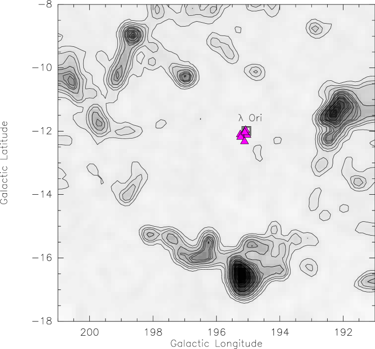
Figure 2: As in Fig. 1, but for the $\lambda^{1}$ Ori stars (triangles). The position of $\lambda$ Ori is shown by an open square ($l\sim 195$°, $b\sim-$12°).

2.2 Observations and data reduction

The observations were carried out in October 2008–January 2010 with flames (Pasquini et al. 2002) on UT2 Telescope. We observed both 25 Ori and $\lambda$ Ori using the fiber link to the red arm of uves. We allocated four fibers to the 25 Ori sample, and two or four fibers to the $\lambda$ Ori sample (depending on the pointing), leaving from two to six fibers for sky acquisition. We used the CD#3 cross-disperser covering the range 4770–6820 Å at the resolution $R=47\,000$, allowing us to select 70+9 Fe i+Fe ii lines, as well as 57 lines of other elements (Sect. 3.4).

In the end, the 25 Ori targets were observed in two different pointings, each including four stars, with no overlap. For each pointing, we obtained four 45 minutes exposures, resulting in a total integration time of 3 hours each. Two pointings were also necessary to observe the $\lambda$ Ori targets. The pointings included four and two stars, and each field was observed three times, for a total exposure time of 2.3 hours each. The log book of the observations is given in Table 2.

For a detailed description of the instrumental setup and data reduction, we refer to Biazzo et al. (2011; and references therein). Ultimately, the typical signal-to-noise ratio ($S/N$) of the co-added spectra in the region of the Li-$\lambda$6708 Å line was 30–80 for 25 Ori and 30–150 for $\lambda$ Ori (see Table 3).

Table 1: Sample stars.

25 Ori
Stara	$V$	$J$	$K$	Sp.T.	Classb	$V_{\rm rad}$
	(mag)	(mag)	(mag)			(km/s)
CVSO35	14.72	11.46	10.35	K7	C	18.8
CVSO207	13.63	11.35	10.56	K4	W	24.2
CVSO211	13.98	11.78	11.06	K5	W	19.4
CVSO214	13.42	11.43	10.74	K2	W	19.1
CVSO259	14.93	12.25	11.40	K7.25	W	…
CVSO260	…	12.57	11.70	M0.6	W	…
CVSO261	…	12.71	11.83	M0	W	…
CVSO262	13.84	11.26	10.45	…	…	…

$\lambda$ Ori
Stara	$V$	$J$	$K$	Sp.T.	Classb	$V_{\rm rad}$
	(mag)	(mag)	(mag)			(km/s)
DM07	13.01	10.80	10.13	…	DL	25.48
DM14	15.18	12.07	11.19	K7	DL	25.66, 27.72
DM26	13.02	10.95	10.30	…	EV	24.96
DM21	14.80	11.66	10.84	…	DL	23.65
CFHT6	13.97	11.54	10.65	…	DL	…
CFHT12	14.09	11.82	10.80	…	DL	…

^a Star names from the following sources: CVSO = CIDA Variability Survey of Orion (Briceño et al. 2005); DM = Dolan & Mathieu (1999); CFHT = Canada-France-Hawaii Telescope optical survey (Barrado et al. 2004).
^b W: Weak-Lined T Tauri; C: Classical T Tauri; DL: Disk-Less; EV: EVolved disk.

Table 2: Log of the observations.

$\alpha$	$\delta$	Date	UT	$t_{\rm exp}$	#
(h:m:s)	(°: ′ : ″)	(d/m/y)	(h:m:s)	(s)	(stars)
25 Ori
05:25:14	01:45:32	12/10/2008	07:17:02	2775	4
05:25:14	01:45:32	16/01/2009	02:20:23	2775	4
05:25:14	01:45:32	17/01/2009	00:54:27	2775	4
05:25:14	01:45:32	19/01/2009	00:37:23	2775	4
05:28:06	02:51:36	21/01/2009	00:52:22	2775	4
05:28:06	02:51:36	21/01/2009	01:40:26	2775	4
05:28:06	02:51:36	27/11/2008	04:58:42	2775	4
05:28:06	02:51:36	29/11/2008	06:27:28	2775	4
$\lambda$ Ori
05:34:33	09:44:01	12/12/2009	03:16:07	2775	4
05:34:33	09:44:01	12/12/2009	04:08:18	2775	4
05:34:33	09:44:01	14/12/2009	03:50:03	2775	4
05:35:07	09:54:55	14/12/2009	04:49:03	2775	2
05:35:07	09:54:55	15/12/2009	03:11:49	2775	2
05:35:07	09:54:55	07/01/2010	03:33:58	2775	2

Table 3: S/N ratios, radial velocities, luminosities, and masses.

25 Ori
Star	$S/N$	$V_{\rm rad}$	Notesa	$L$	$M^{\rm in}$
		(km/s)		($L_{\odot}$)	($M_{\odot}$)
CVSO35	70	19.8$\pm$1.2	M	…	…
CVSO207	70	18.6$\pm$0.6	M	0.64	1.06
CVSO211	70	21.0$\pm$0.4	M	0.44	0.92
CVSO214	70	20.1$\pm$0.2	M	0.62	1.02
CVSO259	50	18.9$\pm$0.8	M	0.27	0.74
CVSO260	30	19.2$\pm$0.6	M	…	…
CVSO261	30	19.8$\pm$0.6	M	…	…
CVSO262	80	19.2$\pm$1.0	M	0.67	1.07

$\lambda$ Ori
Star	$S/N$	$V_{\rm rad}$	Notesa	$L$	$M^{\rm in}$
		(km/s)		($L_{\odot}$)	($M_{\odot}$)
DM07	150	25.3$\pm$0.2	M	1.63	1.35
DM14	60	26.6$\pm$0.4	M	0.46	0.77
DM26	120	28.0$\pm$0.2	M	1.44	1.22
DM21	50	25.4$\pm$1.2	M	0.67	0.86
CFHT6	30	26.8$\pm$0.6	PB	0.79	0.82
”	”	31.1$\pm$0.5	”	”	”
CFHT12	60	$-$3.3$\pm$2.5	NM	…	…

^a M = Member; NM = Non-Member; PB = Probable Binary.

3 Analysis and results

3.1 Radial velocity measurements and membership

We measured radial velocities (RVs) in each observing night, to identify possible non-members and binaries. Since we could not acquire any template spectrum, we first chose for both 25 Ori and $\lambda$ Ori the stars with the spectra at highest $S/N$, low $v\sin i$ ($<$15 km s^-1), available RV measurements from the literature, and without any accretion signature. In particular, we considered CVSO211 for 25 Ori and DM14 for $\lambda$ Ori and followed the method explained in Biazzo et al. (2011). We obtained $V_{\rm rad}=$21.0$\pm$0.4 km s^-1 for CVSO211, while for DM14 we found $V_{\rm rad}=$26.6$\pm$0.4 km s^-1. These values are close to the values of $V_{\rm rad}=$19.4$\pm$0.5 km s^-1 and $V_{\rm rad}=$27.72$\pm$0.18 km s^-1 obtained by Briceño et al. (2007) and Sacco et al. (2008), respectively. Using these two templates, we measured the heliocentric RV of all our targets using the task fxcor of the IRAF package rv, following the prescriptions given by Biazzo et al. (2011).

All our stars were characterized by single peaks of the cross-correlation function. For all measurements with RV of different nights in agreement within $2\sigma$, we computed a mean RV as the weighted average of the different values. Only the star CFHT6 in $\lambda$ Ori shows evidence of binarity, with RV measurements around $V_{\rm rad}=$26.8 km s^-1 (in December 2009) and $V_{\rm rad}=$31.1 km s^-1 (in January 2010). Final radial velocities are listed in Table 3.

We find that all the 25 Ori stars are members with a cluster distribution centered at $<V_{\rm rad}>=19.6\pm 0.8$ km s^-1 (Fig. 3, Table 3), i.e. very close to the peak of $<V_{\rm rad}>=19.7\pm 1.7$ km s^-1 found by Briceño et al. (2007). In particular, the four new PMS stars off to the north-east of 25 Ori (CVSO259,260,261,262) share the same radial velocity of the cluster members from Briceño et al. (2007), consistent with being members of this stellar aggregate. Although four stars represent a small number statistics, this result supports the suggestion made by Briceño et al. (2007) that 25 Ori extends further north than implied by the map in their Fig. 5. The full photometric census of 25 Ori will be presented in Briceño et al. (2011, in preparation). All the $\lambda$ Ori stars are members, with the exception of CFHT12, as also suggested by Barrado et al. (2004) from photometric selection criteria. Excluding CFHT6 and CFHT12, we find a mean $\lambda$ Ori RV of $V_{\rm rad}=$26.3$\pm$1.3 km s^-1, in good agreement with the cluster distribution centered at $<V_{\rm rad}>=27.03\pm 0.49$ km s^-1 (Sacco et al. 2008) .

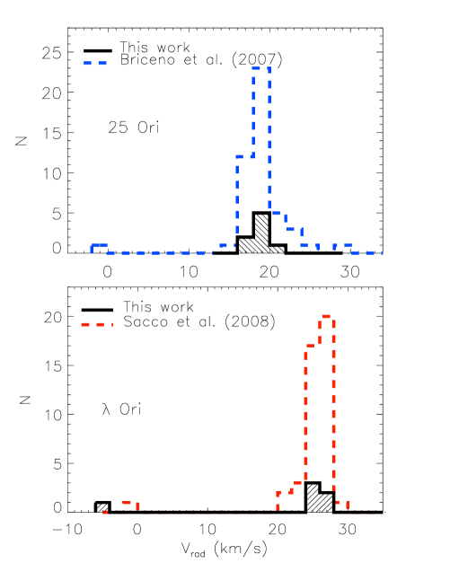
Figure 3: Radial velocity distributions (solid lines) of all the targets in 25 Ori (upper panel) and $\lambda$ Ori (lower panel). The dashed lines represent the distribution obtained by Briceño et al. (2007) for 47 stars in 25 Ori and by Sacco et al. (2008) for 45 members in $\lambda$ Ori.

3.2 Final sample for elemental analysis

Unfortunately, some of the stars are not suitable for abundance analysis. In particular, CVSO35 is a very cool accreting star (classified as CTTS by Briceño et al. 2005), for which the abundance determination through equivalent widths is not reliable. Moreover, CVSO260 and CVSO261 have low $S/N$ spectra ($\raisebox{-2.15277pt}{$\>\stackrel{{\scriptstyle\textstyle<}}{{\sim}}\>$}40$) and low effective temperature ($T_{\rm eff}\raisebox{-2.15277pt}{$\>\stackrel{{\scriptstyle\textstyle<}}{{\sim}}\>$}$4000 K). In these $T_{\rm eff}$ regime, strong molecular bands do not allow one to derive accurate EWs. As a result, we performed abundance measurements in ten stars, five in 25 Ori and five in $\lambda$ Ori. In Figs. 4 and 5 we display the co-added spectra of these stars in the spectral region (6220–6260 Å) containing several features used to derive the effective temperature through line-depth ratios (Sect. 3.3), and to measure the elemental abundances (Sect. 3.4).

Figure 4: Portion of spectra of the targets in 25 Ori used for the abundance determination. The values of $T_{\rm eff}^{\rm SPEC}$ are given for each star.

Figure 5: As in Fig. 4, but for $\lambda$ Ori.

3.3 Initial temperature and surface gravity

Since effective temperatures from the literature were not available for all our targets, we used as initial the values ($T_{\rm eff}^{\rm LDR}$) derived using the method based on line-depth ratios (Gray & Johanson 1991). We followed the prescriptions given by Biazzo et al. (2011) and obtained the values listed in Table 4 and plotted in Fig. 6.

As for surface gravity, the initial gravity ($\log g^{\rm in}$ in Table 4) was obtained from the relation between mass, luminosity, and effective temperature: $\log g=4.44+\log(M/M_{\odot})+4\log(T_{\rm eff}/5770)-\log(L/L_{\odot})$. Effective temperatures were set to our $T_{\rm eff}^{\rm LDR}$ (see Table 4). Stellar luminosities (Table 3), were computed from a relationship between the absolute bolometric magnitude, the $J$ absolute magnitude ($M_{J}$), and the $(V-K)$ color index given by Kenyon & Hartmann (1995) for late-type stars, considering $M_{\rm bol}^{\odot}=4.64$ as solar bolometric magnitude (Cox 2000). The value of $M_{J}$ was obtained adopting a distance of 330 pc for 25 Ori (Briceño et al. 2005) and 400 pc for $\lambda$ Ori (Murdin & Penston 1977), respectively. We used as mean interstellar extinctions the values of $A_{V}=0.29$ given by Briceño et al. (2007) for 25 Ori and $A_{J}=0.106$ for $\lambda$ Ori (Barrado et al. 2004). Initial masses ($M^{\rm in}$ in Table 3) were estimated from the isochrones of Palla & Stahler (1999) at given stellar $M_{J}$ and $T_{\rm eff}^{\rm LDR}$. The HR diagrams for both samples are shown in Fig. 7, together with the Palla & Stahler (1999) tracks and isochrones. The 25 Ori stars show an age around 10 Myr, with the exception of one member, which is marginally older. Three of the $\lambda$ Ori targets are 3–5 Myr old, while the other two are slightly older. Both samples show ages in agreement with previous studies (see Dolan & Mathieu 2001 for $\lambda$ Ori and Briceño et al. 2007 for 25 Ori).

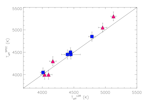
Figure 6: Spectroscopic effective temperatures ($T_{\rm eff}^{\rm SPEC}$) derived by imposing the excitation equilibrium versus effective temperatures obtained through line-depth ratios ($T_{\rm eff}^{\rm LDR}$). The squares and triangles refer to 25 Ori and $\lambda$ Ori, respectively.

Table 4: Astrophysical parameters and elemental abundances derived from spectroscopic analysis.

Star	$T_{\rm eff}^{\rm LDR}$	$T_{\rm eff}^{\rm SPEC}$	$\tiny{\log g}^{\rm in}$	$\tiny{\log g}^{\rm SPEC}$	$\xi$	[Fe i/H]	[Fe ii/H]	[Na/Fe]	[Al/Fe]	[Si/Fe]	[Ca/Fe]	[Ti i/Fe]	[Ti ii/Fe]	$<$[Ti/Fe]$>$	[Ni/Fe]
	(K)	(K)			(km/s)
25 Ori
CVSO207	4447$\pm$48	4600	4.2	4.1	1.7	$-$0.10$\pm$0.09(34)	$-$0.07$\pm$0.11(4)	0.03$\pm$0.10(1)	0.16$\pm$0.11(2)	0.06$\pm$0.21(5)	0.05$\pm$0.09(3)	$-$0.02$\pm$0.16(6)	0.00$\pm$0.10(2)	$-$0.01$\pm$0.13	$-$0.04$\pm$0.11(13)
CVSO211	4399$\pm$47	4550	4.3	4.2	1.4	$-$0.05$\pm$0.09(43)	$-$0.03$\pm$0.13(3)	$-$0.04$\pm$0.09(1)	0.08$\pm$0.12(2)	0.08$\pm$0.24(5)	0.01$\pm$0.10(3)	$-$0.03$\pm$0.12(7)	0.10$\pm$0.10(2)	0.04$\pm$0.13	$-$0.02$\pm$0.12(15)
CVSO214	4787$\pm$52	4900	4.3	4.2	2.1	$-$0.08$\pm$0.06(41)	$-$0.06$\pm$0.09(5)	0.08$\pm$0.06(1)	0.12$\pm$0.13(2)	0.10$\pm$0.10(3)	0.06$\pm$0.08(3)	0.01$\pm$0.10(9)	0.00$\pm$0.08(3)	0.01$\pm$0.13	$-$0.02$\pm$0.13(22)
CVSO259	4011$\pm$42	4050	4.2	…	1.4	0.01$\pm$0.16(32)	…	$-$0.26$\pm$0.16(1)	$-$0.06$\pm$0.22(2)	0.06$\pm$0.16(2)	$-$0.20$\pm$0.16(2)	$-$0.28$\pm$0.19(8)	…	…	0.01$\pm$0.21(6)
CVSO262	4453$\pm$150	4450	4.1	…	1.9	$-$0.01$\pm$0.09(23)	…	…	$-$0.05$\pm$0.09(2)	…	$-$0.04$\pm$0.15(1)	$-$0.21$\pm$0.21(3)	…	…	$-$0.02$\pm$0.17(2)
25 Ori						$-$0.05$\pm$0.05	$-$0.05$\pm$0.02	0.02$\pm$0.06	0.08$\pm$0.08	0.08$\pm$0.02	0.02$\pm$0.05			0.01$\pm$0.02	$-$0.02$\pm$0.02
$\lambda$ Ori
DM07	4956$\pm$67	5050	4.1	4.2	2.1	0.00$\pm$0.07(39)	0.02$\pm$0.04(3)	0.06$\pm$0.08(1)	0.15$\pm$0.01(2)	0.13$\pm$0.03(4)	$-$0.03$\pm$0.09(2)	0.00$\pm$0.09(7)	0.12$\pm$0.17(4)	0.06$\pm$0.20	$-$0.01$\pm$0.07(14)
DM14	4037$\pm$64	4000	4.0	…	1.4	0.01$\pm$0.08(31)	…	$-$0.26$\pm$0.09(1)	$-$0.13$\pm$0.05(2)	0.18$\pm$0.19(4)	$-$0.21$\pm$0.09(2)	$-$0.23$\pm$0.12(6)	0.45$\pm$0.14(2)	0.11$\pm$0.18	0.08$\pm$0.13(16)
DM21	4167$\pm$55	4300	4.0	…	1.4	0.02$\pm$0.08(19)	…	$-$0.13$\pm$0.13(1)	$-$0.01$\pm$0.09(2)	0.06$\pm$0.43(2)	$-$0.09$\pm$0.13(1)	$-$0.05$\pm$0.08(3)	…	…	$-$0.03$\pm$0.15(3)
DM26	5128$\pm$40	5300	4.2	…	2.3	0.01$\pm$0.10(21)	…	…	0.23$\pm$0.01(2)	0.04$\pm$0.18(3)	…	0.06$\pm$0.10(5)	…	…	0.01$\pm$0.13(5)
CFHT6	4099$\pm$58	4000	3.8	…	1.6	$-$0.01$\pm$0.14(18)	…	$-$0.23$\pm$0.16(1)	$-$0.20$\pm$0.09(2)	0.14$\pm$0.17(1)	$-$0.26$\pm$0.14(2)	$-$0.29$\pm$0.20(3)	0.26$\pm$0.19(1)	$-$0.02$\pm$0.28	0.04$\pm$0.17(5)
$\lambda$ Ori						0.01$\pm$0.01	0.02$\pm$0.04	0.06$\pm$0.08	0.19$\pm$0.06	0.11$\pm$0.06	$-$0.03$\pm$0.09			0.05$\pm$0.06	0.02$\pm$0.04

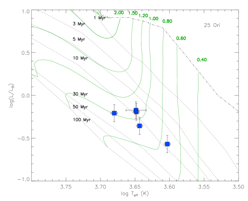
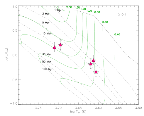
Figure 7: HR diagram of the members of 25 Ori (upper panel; squares) and $\lambda$ Ori (lower panel; triangles) where the abundance analysis was done. The Palla & Stahler (1999) PMS evolutionary tracks are displayed with the labels representing their masses (solid lines). Similarly, the birthline and isochrones (from 1 to 30 Myr) are shown with dash-dotted and dotted lines, respectively.

3.4 Stellar abundance measurements

Stellar abundances were measured following the prescriptions given by Biazzo et al. (2011). We briefly list the main steps, but we refer to that paper for a detailed description of the method.

• We performed abundance analysis in local thermodynamic equilibrium (LTE) conditions using equivalent widths and the 2002 version of MOOG (Sneden 1973). The radiative and Stark broadening were treated in a standard way, while, for collisional broadening, we used the Unsöld (1955) approximation.

• Kurucz (1993) and Brott & Hauschildt (2010, private comm.) grid of plane-parallel model atmospheres were used for warm ($>$4400 K) and cool ($\>\stackrel{{\scriptstyle\textstyle<}}{{\sim}}\>$4400 K) stars, respectively.

• Equivalent widths were measured by direct integration or by Gaussian fit using the IRAF splot task.

• We adopted the line list of Biazzo et al. (2011), adding other useful iron lines (see Table 5) taken from Santos et al. (2008).

• After removing lines with $EW>150$ mÅ, likely saturated and most affected by the treatment of damping, we applied a $2\sigma$ clipping rejection.

• Although we do not expect high levels of veiling in our sample, we searched for any possible excess emission. We found that all stars had veiling levels consistent with zero, confirming that this quantity is not an issue in our abundance measurements.

• Our study is performed differentially with respect to the Sun. We analyzed the uves solar spectrum adopting $T_{\rm eff}=5770$ K, $\log g=4.44$, $\xi=1.1$ km s^-1 (see Randich et al. 2006). We obtained $\log n{\rm({Fe\textsc{i}})}=7.52\pm 0.02$ and $\log n{\rm({Fe\textsc{i}})}=7.51\pm 0.02$ with Kurucz and Brott & Hauschildt model atmospheres, respectively. For the iron solar abundance of each line, see Biazzo et al. (2011, and references therein), and Table 5. The solar abundances of all the other elements are listed in Table 3 of Biazzo et al. (2011), since we used the same line list.

Table 5: Wavelength, excitation potential, oscillator strength, equivalent width, and abundance obtained with ATLAS (Kurucz 1993) and GAIA (Brott & Hauschildt 2010, private comm.) models for the iron lines taken from Santos et al. (2008) are listed.

$\lambda$	$\chi$	$\log gf$	$EW$	$\log n_{\rm ATLAS}$	$\log n_{\rm GAIA}$
(Å)	(eV)		(mÅ)
5322.05	2.28	$-$2.90	62.3	7.49	7.47
5852.22	4.55	$-$1.19	41.2	7.50	7.48
5855.08	4.61	$-$1.53	22.2	7.46	7.45
6027.06	4.08	$-$1.18	63.7	7.48	7.46
6079.01	4.65	$-$1.01	48.3	7.54	7.52
6089.57	5.02	$-$0.88	36.1	7.51	7.49
6151.62	2.18	$-$3.30	51.1	7.47	7.47
6608.03	2.28	$-$3.96	17.8	7.46	7.46
6646.94	2.61	$-$3.94	11.0	7.51	7.51
6710.32	1.48	$-$4.82	17.2	7.49	7.50

3.4.1 Stellar parameters

Effective temperatures were also determined by imposing the condition that the Fe i abundance does not depend on the line excitation potentials. The initial value of the effective temperature ($T_{\rm eff}^{\rm LDR}$), and the final values ($T_{\rm eff}^{\rm SPEC}$) are listed in Table 4 and plotted in Fig. 6. The temperatures obtained with both methods are in good agreement (mean difference of $\sim$100 K), with $T_{\rm eff}^{\rm SPEC}$ higher on average than $T_{\rm eff}^{\rm LDR}$.

The microturbulence velocity $\xi$ was determined by imposing that the Fe i abundance is independent on the line equivalent width. The initial value was set to 1.5 km s^-1, and the final values are listed in Table 4.

The surface gravity was determined by imposing the ionization equilibrium of Fe i/Fe ii. With the exception of CVSO259 and CVSO262 with few suitable lines in the spectra, we were able to constrain the gravity for the stars in 25 Ori ($\log g^{\rm SPEC}$ in Table 4). In the case of $\lambda$ Ori, only DM07 shows enough Fe ii lines to allow a spectroscopic measurement of the gravity.

3.4.2 Errors

As described in Biazzo et al. (2011), elemental abundances are affected by random (internal) and systematic (external) errors.

In brief, sources of internal errors include uncertainties in atomic parameters, stellar parameters, and line equivalent widths, where the former should cancel out when the analysis is carried out differentially with respect to the Sun, as in our case.

Errors due to uncertainties in stellar parameters were estimated by assessing errors in $T_{\rm eff}$, $\xi$, and $\log g$, and by varying each parameter separately, while keeping the other two unchanged. We found that variations in $T_{\rm eff}$ larger than 60 K would introduce spurious trends in $\log n{\rm({Fe\textsc{i}})}$ versus $\chi$; variations in $\xi$ larger than 0.2 km s^-1 would result in significant trends of $\log n{\rm({Fe\textsc{i}})}$ versus $EW$, and variations in $\log g$ larger than 0.2 dex would lead to differences between $\log n{\rm({Fe\textsc{i}})}$ and $\log n{\rm({Fe\textsc{ii}})}$ larger than 0.05 dex. Errors in abundances due to uncertainties in stellar parameters are summarized in Table 6 for one of the coolest stars (DM14) and for the warmest target (DM07).

Random errors in EW are well represented by the standard deviation around the mean abundance determined from all the lines. When only one line was measured, the abundance error is the standard deviation of three independent EW measurements. In Table 4 these errors are listed together with the number of lines used (in brackets).

As for the external error, the biggest one is given by the abundance scale, which is mainly influenced by errors in model atmospheres. As pointed out by Biazzo et al. (2011), this error source is negligible, because we used for both clusters the same procedure and instrument set-up to measure the elemental abundances.

Table 6: Internal errors in abundance determination due to uncertainties in stellar parameters for one of the coolest star (namely, DM14) and for the warmest star (DM07). Numbers refer to the differences between the abundances obtained with and without the uncertainties in stellar parameters.

DM14	$T_{\rm eff}$=4000 K	$\log g=4.0$	$\xi=1.4$ km/s
$\Delta$	$\Delta T_{\rm eff}=-/+60$ K	$\Delta\log g=-/+0.2$	$\Delta\xi=-/+0.2$ km/s
$[$Fe i/H$]$	0.05/$-$0.03	$-$0.04/0.06	0.05/$-$0.04
$[$Na/Fe$]$	$-$0.09/0.06	0.07/$-$0.09	$-$0.03/0.01
$[$Al/Fe$]$	$-$0.05/0.03	0.02/$-$0.03	$-$0.03/0.01
$[$Si/Fe$]$	0.04/$-$0.06	$-$0.05/0.04	$-$0.05/0.03
$[$Ca/Fe$]$	$-$0.08/0.07	0.07/$-$0.07	0.01/$-$0.01
$[$Ti i/Fe$]$	$-$0.07/0.06	0.03/$-$0.04	0.04/$-$0.06
$[$Ti ii/Fe$]$	0.02/$-$0.03	$-$0.08/0.06	$-$0.03/0.02
$[$Ni/Fe$]$	0.00/$-$0.01	$-$0.02/0.02	$-$0.01/0.01
DM07	$T_{\rm eff}$=5050 K	$\log g=4.2$	$\xi=2.1$ km/s
$\Delta$	$\Delta T_{\rm eff}=-/+60$ K	$\Delta\log g=-/+0.2$	$\Delta\xi=-/+0.2$ km/s
$[$Fe i/H$]$	$-$0.01/0.02	$-$0.02/0.02	0.06/$-$0.05
$[$Fe ii/H$]$	0.05/$-$0.04	$-$0.14/0.10	0.03/$-$0.02
$[$Na/Fe$]$	$-$0.03/0.01	0.03/$-$0.05	$-$0.05/0.03
$[$Al/Fe$]$	$-$0.02/0.01	0.03/$-$0.03	$-$0.03/0.03
$[$Si/Fe$]$	0.02/$-$0.04	$-$0.04/0.00	$-$0.05/0.03
$[$Ca/Fe$]$	$-$0.03/0.02	0.04/$-$0.04	$-$0.02/0.01
$[$Ti i/Fe$]$	$-$0.06/0.04	0.02/$-$0.02	0.01/$-$0.01
$[$Ti ii/Fe$]$	0.03/$-$0.03	$-$0.08/0.06	$-$0.05/0.04
$[$Ni/Fe$]$	0.01/$-$0.02	$-$0.03/0.01	$-$0.03/0.02

3.5 Elemental abundances

We measured the abundances of iron, sodium, aluminum, silicon, calcium, titanium, and nickel. Our final abundances are listed in Table 4.

In Fig. 8 we show the [Fe/H] and [X/Fe] ratios as a function of $T_{\rm eff}^{\rm SPEC}$ for 25 Ori and $\lambda$ Ori. The figure shows that there is no star-to-star variation in all elements in both groups with the exceptions of the elements where NLTE effects are present, namely Na, Al, Ca, and Ti. In particular, due to their young age, cluster stars are characterized by high levels of chromospheric activity and are more affected by NLTE over-ionization, which cause a decreasing trend towards lower temperatures of neutral species of elements with low ionization potential (see D’Orazi & Randich 2009; Biazzo et al. 2011, and references therein, for thorough discussions of this issue).

For 25 Ori, the mean iron abundance is $<$[Fe/H]$>=-0.05\pm 0.05$, while for $\lambda$ Ori we find $<$[Fe/H]$>$$=0.01\pm 0.01$.

Fig. 8 also shows that stars of 25 Ori and $\lambda$ Ori are characterized by homogeneous, close-to-solar elemental abundances.

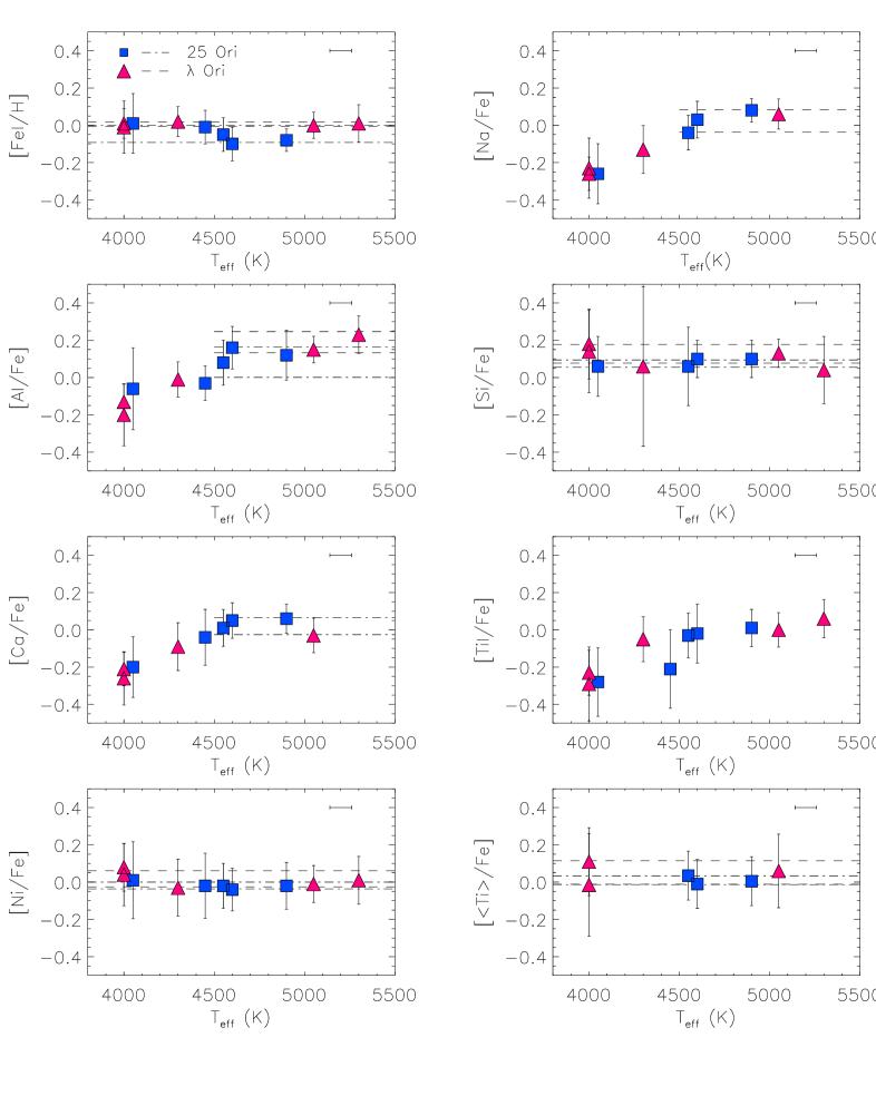
Figure 8: [X/Fe] versus $T_{\rm eff}^{\rm SPEC}$ for our 25 Ori (squares) and $\lambda$ Ori (triangles) members. Mean abundances values for elements affected by NLTE effects were computed considering the stars with $T_{\rm eff}^{\rm SPEC}>4400$ K, while $\pm 1\sigma$ dispersions are shown by dash-dotted lines for 25 Ori and dotted lines for $\lambda$ Ori. The dashed and dash-dotted lines show the $\pm 1\sigma$ values from the mean 25 Ori and $\lambda$ Ori abundances, respectively. The horizontal error bar in all plots represents the typical uncertainty in $T_{\rm eff}^{\rm SPEC}$.

4 Discussion

4.1 Metallicity distribution in Orion

In Fig. 9 and in Table 7 we show the [Fe/H] distribution of the Orion subgroups, namely the Orion Nebula Cluster (ONC), OB1b, OB1a (Biazzo et al. 2011), $\sigma$ Ori (González-Hernández et al. 2008), $\lambda$ Ori, and 25 Ori (this work). As can be seen, the Orion complex seems to be slightly inhomogeneous, with the iron abundance ranging from $-$0.13$\pm$0.03 (the ONC) to 0.01$\pm$0.01 ($\lambda$ Ori), and an internal dispersion of $\sim 0.05$ dex. Interestingly, while $\lambda$ Ori has an iron abundance identical to solar, all the Orion subgroups are below solar. It is also remarkable that the youngest object, the ONC, has the lowest value at all. These results seem to exclude a direct and significant amount of contamination between neighboring (or adjacent) regions, or an increase of iron abundance with age, as naïvely expected in a SN-driven abundance enriched scenario (see Biazzo et al. 2011, and references therein). This is also supported by the velocity dispersion observed in the Orion subgroups, which is around 0.5–2.7 km/s, or $\sim$0.5–2 pc/Myr (see Table 7). This means that the members of the subgroups would have moved at most (if on ballistic orbits) by only a few pc for the ONC and up to $\sim$10 pc for the oldest ones. Excluding systematic biases in the analysis, this small dispersion in Orion may be the result of several effects. $i)$ Different and independent episodes of star formation between $\lambda$ Ori and the other Orion subgroups analyzed. The former formed $\sim 8-10$ Myr ago from a supernova explosion close to the present $\lambda^{1}$ Ori position (Dolan & Mathieu 1999, 2001), while the other regions are the result of sequential star formation triggered by supernova type-II events in the OB1a association (Preibisch & Zinnecker 2006). $ii)$ Large-scale formation processes on $\sim 1$ kpc scale may lead to chemically inhomogenous gas inside the giant molecular cloud (Elmegreen 1998). A quick onset of star formation in clumps of the molecular clouds born under turbulent conditions implies that any non-uniformity of abundances may enter the cloud, from an initial non-uniform pre-cloud gas or from the background Galactic gradient. In this case there is not enough time for uniform mixing before star formation, and the range of cloud metallicity inhomogeneity may reach a level of $\pm 0.05$ dex. Even if the spatial scales involved in the formation of the Orion complex are most likely smaller (Hartmann & Burkert 2007), the presence of inhomogeneous gas in the interstellar medium could contribute to the observed small dispersions.

These results are encouraging, because for many years our knowledge about the chemical composition in the Orion complex from early-B main sequence stars (Cunha & Lambert 1992, 1994) and late-type stars (Cunha et al. 1998; D’Orazi et al. 2009) was characterized by highly inhomogeneous abundances, with group-to-group differences of $\sim 0.40$ dex in oxygen, $\sim 0.30-0.40$ dex in silicon, and $\sim 0.10$ dex in iron. These large spreads have been interpreted as the chemical signature of self-enrichment inside the Orion OB association by ejecta of type-II SNe from massive stars. Our results change this picture. Also, the new revision of the abundances of B-type stars in Orion OB1a, b, c, d performed by Simón-Díiaz (2010) and the good agreement between our own and the Santos et al. (2008) values for low-mass stars indicate a very low dispersion in the abundances of oxygen, silicon, nickel, and iron, with the Orion Nebula Cluster representing the most metal-poor subgroup. Note that, as pointed out by Simón-Díiaz (2010) and Biazzo et al. (2011), the small group-to-group elemental abundance dispersions are smaller than the internal errors in measurements.

Why is the ONC so significantly different from the other regions is an interesting question that should be addressed in the future. The cluster is located at the tip of a loose molecular cloud that contains an extended population of embedded and optically visible low-mass stars (Megeath et al. 2005). Their properties have been recently analyzed by Fang et al. (2009), who provide useful candidates to be observed for abundance measurements. Then, one can verify if the ONC is just an anomaly or if it shows the same abundance of the present Giant Molecular Cloud. Similarly, the situation in $\lambda$ Ori is favorable to study a possible link between what we find close to the $\lambda^{1}$ Ori star and the chemical abundances of the current generation of young stars located in the vicinity of the molecular gas clumps shown in Fig. 2. For example, Dolan & Mathieu (2001) provide the properties of the CTTS/WTTS in these regions that can then be observed for metallicity measurements.

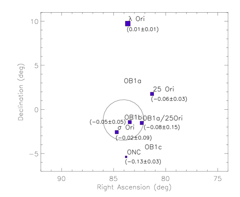
Figure 9: Iron abundance distribution of members of the Orion complex (ONC, OB1b, OB1a, $\sigma$ Ori, 25 Ori, and $\lambda$ Ori) taken from the most recent literature (González-Hernández et al. 2008; Biazzo et al. 2011) and this work. Symbols with different size denote three different metallicity bins: [Fe/H]$\leq-0.10$, $-0.09\leq$[Fe/H]$\leq 0.00$, and [Fe/H]$>0.00$, from the smallest to the largest size. The central bin corresponds to the average metallicity of the Orion complex $\pm 1\sigma$. The mean metallicity of each subgroup is written in parenthesis. The circle outlines the Briceño et al. (2005) boundary of the Orion OB subgroups.

Table 7: Mean iron abundance of low-mass stars, velocity dispersion, and age range of the Orion subgroups.

SFR	[Fe/H]	Reference	# stars	$\delta V_{\rm rad}$	Reference	Age	Reference
				(km/s)		(Myr)
$\sigma$ Ori	$-$0.02$\pm$0.09	González-Hernández et al. (2008)	8	0.9	Sacco et al. (2008)	2–3	Walter et al. (2008)
ONC	$-$0.13$\pm$0.03	Biazzo et al. (2011)	10	3.1	Fürész et al. (2009)	2–3	Da Rio et al. (2010)
OB1b	$-$0.05$\pm$0.05	Biazzo et al. (2011)	4	1.9	Briceño et al. (2007)	4–6	Briceño et al. (2007)
OB1a/25 Ori	$-$0.08$\pm$0.15	Biazzo et al. (2011)	1	$\sim$2	Briceño et al. (2007)	7–10	Briceño et al. (2005)
25 Ori	$-$0.05$\pm$0.05	This work	5	1.7	Briceño et al. (2007)	7–10	Briceño et al. (2005)
$\lambda$ Ori	0.01$\pm$0.01	This work	5	0.5	Sacco et al. (2008)	5–10	Dolan & Mathieu (2002)

4.2 SFR abundances in the Galactic disk

Each component of our Galaxy (bulge, halo, thin and thick disk) presents a characteristic abundance pattern of elements (such as iron-peak and $\alpha$-elements) with respect to iron. The observed differences reflect a variety of star formation histories. One would expect that SFRs show a similar pattern as thin disk stars, unless the gas from which they have formed has undergone a peculiar enrichment. In order to check if this is indeed true, we compare [X/Fe] ratios versus [Fe/H] trends for SFRs (King et al. 2000; Santos et al. 2008; González-Hernández et al. 2008; Biazzo et al. 2011; D’Orazi et al. 2011) with studies of nearby field stars of the thin Galactic disk (Soubiran & Girard 2005).

Fig. 10 shows an overall good agreement between the [X/Fe] versus [Fe/H] distribution of SFRs and nearby field stars. A more detailed discussion on the different groups of elements is provided below:

The $\alpha$ elements Si, Ca, and Ti

The $\alpha$ elements are mostly produced in the aftermath of explosions of type II supernovae, with small contribution from type Ia SNe. On average, [Si/Fe] in SFRs seems to be slightly higher than the Sun (Fig. 10). Given the dispersion in Si abundance of the SFRs, it is fully consistent with the distribution of the field stars of the thin disk. The behaviour of [Ca/Fe] and [Ti/Fe] ratios versus [Fe/H] is similar to those reported by Soubiran & Girard (2005) for field stars with $-0.2\raisebox{-2.15277pt}{$\>\stackrel{{\scriptstyle\textstyle<}}{{\sim}}\>$}$[Fe/H]$\raisebox{-2.15277pt}{$\>\stackrel{{\scriptstyle\textstyle<}}{{\sim}}\>$}0.2$.

The slight overabundance in [$\alpha$/Fe] of the SFRs might be the result of the contributions of recent local enrichment due to SNIIe ejecta (occurred in particular in the Orion complex) or of local accretion from enriched gas pre-existing in the nearby thin disk (Elmegreen 1998). In particular, the slight overabundance in Si of SFRs might reflect its larger production during SNII events compared to the calcium and titanium elements (Woosley & Weaver 1995).

The iron-peak element nickel

Most of the iron-peak elements are synthesized by SNIa explosions. The nickel abundance is very close to the solar value, as found for field stars with [Fe/H] between $-0.4$ and 0.0 (Fig. 10).

Other elements: Na and Al

Sodium and aluminum are thought to be mostly a product of Ne and Mg burning in massive stars, through the NeNa and MgAl chains. The [Na/Fe] ratio does not show a trend with [Fe/H], with a mean value close to that of field stars at the same [Fe/H]. Similarly, the Al abundance does not show trend with [Fe/H], but at slightly above-solar values, as for field stars in the solar neighborhood. Its phenomenological behaviour is very similar to the $\alpha$-elements, as indicated by McWilliam (1997).

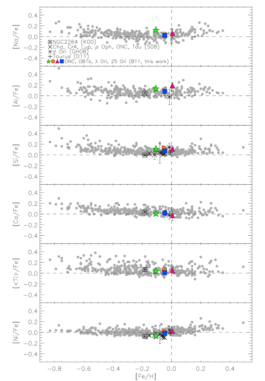
Figure 10: [X/Fe] versus [Fe/H] for SFRs with known high-resolution abundances. The references are: Biazzo et al. (2011; B11), D’Orazi et al. (2011; D11), Santos et al. (2008; S08), King et al. (2000; K00), and González-Hernández et al. (2008; GH08). The errors in [Fe/H] are around 0.02–0.12 dex. The dashed lines mark the solar abundances. The filled dots in the background represent the [X/Fe] distribution of nearby field stars in the Galactic thin disk (Soubiran & Girard 2005).

5 Conclusions

In this paper we have derived homogeneous and accurate abundances of Fe, Na, Al, Si, Ti, Ca, and Ni of two very young clusters, namely 25 Orionis and $\lambda$ Orionis. Our main results can be summarized as follows:

• Stellar properties have been derived for 14 low-mass stars over a relatively wide temperature interval. Four new PMS candidates show kinematics consistent with membership in the 25 Ori cluster.

• $\lambda$ Ori and 25 Ori have mean iron abundances of $0.01\pm 0.01$ and $-0.05\pm 0.05$, respectively, without the presence of metal-rich stars.

• Whereas this should be confirmed based on larger number statistics, our results suggest that no star-to-star variation is present for all elements, with a high degree of homogeneity inside each stellar group.

• Elemental abundances of $\lambda$ Ori, 25 Ori, and other known SFRs agree with those of the Galactic thin disk.

• The Orion complex seems to be characterized by a small group-to-group dispersion, consistent with a different star formation history of each subgroup and an initially inhomogeneous interstellar gas.

• Finally, we note that the close-to-solar metallicity of both 25 Ori and $\lambda$ Ori reinforces the conclusion that none of the SFRs in the solar neighborhood is metal-rich and that metal-rich stars hosting giant planets are likely migrated from the inner part of the Galactic disk to their current location (Santos et al. 2008; Haywood 2008).