Diameters of random circulant graphs

Abstract.

The diameter of a graph measures the maximal distance between any pair of vertices. The diameters of many small-world networks, as well as a variety of other random graph models, grow logarithmically in the number of nodes. In contrast, the worst connected networks are cycles whose diameters increase linearly in the number of nodes. In the present study we consider an intermediate class of examples: Cayley graphs of cyclic groups, also known as circulant graphs or multi-loop networks. We show that the diameter of a random circulant $2k$-regular graph with $n$ vertices scales as $n^{1/k}$, and establish a limit theorem for the distribution of their diameters. We obtain analogous results for the distribution of the average distance and higher moments.

1. Introduction

The diameter of a graph is the largest distance between any pair of vertices, and is a popular measure for the connectedness of a network. Many models of small-world networks, for example, have diameters that grow slowly (i.e., logarithmically) with the total number of nodes [9], [19]. The same phenomenon is observed for a wide variety of other random graph models, and has been proved rigorously in many instances [6], [7], [12], [15], [18], [27], [33]. The worst connected networks are cycles, whose diameters increase linearly with the number of vertices. Here, connectedness is dramatically improved by additionally linking every vertex with a random partner; the logarithmic growth of the diameter is then recovered [8].

In the present paper we consider a more regular generalization, the circulant graphs (often also called multi-loop networks) which comprise an interwoven assembly of cycles (Figs. 1, 2 left). We will show that the diameter of a random $2k$-regular circulant graph with $n$ vertices scales as $n^{1/k}$, and prove a limit theorem for the distribution of diameters of such graphs; the existence of a limit distribution was recently conjectured in [2]. Analogous results hold for the distribution of the average distance in a circulant graph and related quantities, see Sec. 5 for details. It is interesting to note that an algebraic scaling of the diameter has also been observed for the largest connected component of the critical Erdös-Rényi random graph [31]; here the scaling factor is $n^{1/3}$.

We furthermore establish corresponding results for circulant digraphs (cf. Figs. 1, 2 right), where the limit distribution of diameters turns out to coincide with the limit distribution of Frobenius numbers in $d=k+1$ variables studied in [28]. The connection of these two objects has been exploited previously [3], [32], [35], [39]. As for the Frobenius problem [24], the question of calculating the diameter of circulant graphs can be transformed to a problem in the geometry of numbers [11], [41]. We will use a particularly transparent approach that identifies circulant graphs with lattice graphs on flat tori [13], [16], and then employ the ergodic-theoretic method developed in [28] to prove the existence of the limit distribution of diameters.

Let us fix an integer vector ${\text{\boldmath$a$}}=(a_{1},\ldots,a_{k})$ with distinct positive coefficients $0<a_{1}<\ldots<a_{k}\leq\frac{n}{2}$. We construct a graph $C_{n}({\text{\boldmath$a$}})$ with $n$ vertices $0,1,2,\ldots,n-1$, by connecting vertex $i$ and $j$ whenever $|i-j|\equiv a_{h}\bmod n$ for some $h\in\{1,\ldots,k\}$. Because the adjacency matrix of this graph is circulant, $C_{n}({\text{\boldmath$a$}})$ is called a circulant graph. If $a_{k}<\frac{n}{2}$, then $C_{n}({\text{\boldmath$a$}})$ is $2k$-regular, i.e., every vertex has precisely $2k$ neighbours. If $a_{k}=\frac{n}{2}$, then $C_{n}({\text{\boldmath$a$}})$ is $(2k-1)$-regular. It is easy to see that $C_{n}({\text{\boldmath$a$}})$ is connected if and only if $\gcd(a_{1},\ldots,a_{k},n)=1$. In this case $C_{n}({\text{\boldmath$a$}})$ is the (undirected) Cayley graph of $\mathbb{Z}/n\mathbb{Z}$ with respect to the generating set $\{\pm a_{1},\ldots,\pm a_{k}\}$.

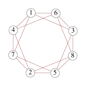
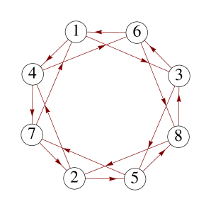
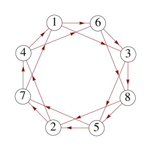
Figure 1. The 4-regular circulant graph $C_{8}(2,3)$ and the circulant digraphs $C_{8}^{+}(2,3)$, $C_{8}^{+}(2,5)$. The corresponding diameters are 2, 3 and 4, respectively.

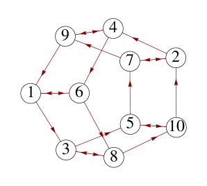
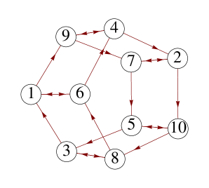
Figure 2. The 3-regular circulant graph $C_{10}(2,5)$ and the circulant digraphs $C_{10}^{+}(2,5)$, $C_{10}^{+}(5,8)$. The corresponding diameters are 3, 5 and 5, respectively.

To construct a directed circulant graph (circulant digraph for short) choose an integer vector ${\text{\boldmath$a$}}=(a_{1},\ldots,a_{k})$ with distinct positive coefficients $0<a_{1}<\ldots<a_{k}<n$. The circulant digraph $C_{n}^{+}({\text{\boldmath$a$}})$ is defined to have an edge from $i$ to $j$ whenever $j-i\equiv a_{h}\bmod n$ for some $h\in\{1,\ldots,k\}$. In $C_{n}^{+}({\text{\boldmath$a$}})$, every vertex has precisely $k$ outgoing and $k$ incoming edges. $C_{n}^{+}({\text{\boldmath$a$}})$ is strongly connected if and only if $\gcd(a_{1},\ldots,a_{k},n)=1$. In this case $C_{n}^{+}({\text{\boldmath$a$}})$ is the directed Cayley graph of $\mathbb{Z}/n\mathbb{Z}$ with respect to the generating set $\{a_{1},\ldots,a_{k}\}$.

Fix a vector ${\text{\boldmath$\ell$}}=(\ell_{1},\ldots,\ell_{k})\in{\mathbb{R}}_{>0}^{k}$. We endow our circulant (di-)graph with a (quasi-)metric by stipulating that the edge from $i$ to $j\equiv i+a_{h}\bmod n$ has length $\ell_{h}$. We denote the corresponding metric graphs by $C_{n}({\text{\boldmath$\ell$}},{\text{\boldmath$a$}})$ and $C_{n}^{+}({\text{\boldmath$\ell$}},{\text{\boldmath$a$}})$, respectively. The distance $d(i,j)$ between two vertices is the length of the shortest path from $i$ to $j$. The diameter is the maximal distance between any pair of vertices,

(1.1) $$\operatorname{diam}=\max_{i,j}d(i,j).$$

To define an ensemble of random circulant graphs, we set

(1.2) $${\mathfrak{F}}^{+}:=\{{\text{\boldmath$x$}}\in{\mathbb{R}}^{k+1}:0<x_{1}<\ldots<x_{k}<x_{k+1}\};\qquad{\mathfrak{F}}:={\mathfrak{F}}^{+}\cap\{x_{k}\leq{\textstyle\frac{1}{2}}x_{k+1}\},$$

and then in the directed case we fix an arbitrary bounded subset ${\mathcal{D}}\subset{\mathfrak{F}}^{+}$ with nonempty interior and boundary of Lebesgue measure zero; in the undirected case we fix an arbitrary bounded subset ${\mathcal{D}}\subset{\mathfrak{F}}$ subject to the same conditions. Denote by $\widehat{\mathbb{N}}^{k+1}$ the set of integer vectors in ${\mathbb{R}}^{k+1}$ with positive coprime coefficients (i.e., the greatest common divisor of all coefficients is one). The numbers $({\text{\boldmath$a$}},n)\in\widehat{\mathbb{N}}^{k+1}$ defining $C_{n}({\text{\boldmath$\ell$}},{\text{\boldmath$a$}})$ or $C_{n}^{+}({\text{\boldmath$\ell$}},{\text{\boldmath$a$}})$ are then picked uniformly at random from the dilated set $T{\mathcal{D}}$ ($T>0$). Note here that $\widehat{\mathbb{N}}^{k+1}\cap T{\mathcal{D}}$ is nonempty for all large $T$; in fact

(1.3) $$\#\big{\{}({\text{\boldmath$a$}},n)\in\widehat{\mathbb{N}}^{k+1}\cap T{\mathcal{D}}\big{\}}\sim\frac{\operatorname{vol}({\mathcal{D}})}{\zeta(k+1)}\,T^{k+1},\qquad\text{as }\>T\to\infty.$$

Our first main theorem shows that the (properly scaled) diameter of a random circulant digraph has a limit distribution which is independent of the choice of ${\mathcal{D}}$. In order to describe this limit distribution, we introduce some further notation. For a given closed bounded convex set $K$ of nonzero volume in $\mathbb{R}^{k}$ and a ($k$-dimensional) lattice $L\subset\mathbb{R}^{k}$, we denote by $\rho(K,L)$ the covering radius of $K$ with respect to $L$, i.e. the smallest positive real number $r$ such that the translates of $rK$ by the vectors of $L$ cover all of $\mathbb{R}^{k}$:

(1.4) $$\rho(K,L)=\inf\bigl{\{}r>0\>:\>rK+L=\mathbb{R}^{k}\bigr{\}}.$$

Let $X_{k}$ be the set of all lattices $L\subset\mathbb{R}^{k}$ of covolume one, and let $\mu_{0}$ be the $\operatorname{SL}(k,\mathbb{R})$ invariant probability measure on $X_{k}$. Also let $\Delta$ be the simplex

(1.5) $$\Delta=\big{\{}{\text{\boldmath$x$}}\in{\mathbb{R}}_{\geq 0}^{k}:x_{1}+\ldots+x_{k}\leq 1\big{\}}.$$

Theorem 1.

Let $k\geq 2$. Then for any ${\text{\boldmath$\ell$}}\in{\mathbb{R}}_{>0}^{k}$ and any bounded set ${\mathcal{D}}\subset{\mathfrak{F}}^{+}$ with nonempty interior and boundary of Lebesgue measure zero, we have convergence in distribution

(1.6) $$\frac{\operatorname{diam}C_{n}^{+}({\text{\boldmath$\ell$}},{\text{\boldmath$a$}})}{(n\ell_{1}\cdots\ell_{k})^{1/k}}\xrightarrow[]{\textup{ d }}\rho(\Delta,L)\qquad\text{as }\>T\to\infty,$$

where the random variable in the left-hand side is defined by taking $({\text{\boldmath$a$}},n)$ uniformly at random in $\widehat{\mathbb{N}}^{k+1}\cap T{\mathcal{D}}$, and the random variable in the right-hand side is defined by taking $L$ at random in $X_{k}$ according to $\mu_{0}$.

Figure 3. Distribution of diameters $n^{-1/k}(\operatorname{diam}C_{n}^{+}({\text{\boldmath$\ell$}},{\text{\boldmath$a$}})+{\text{\boldmath$e$}}\cdot{\text{\boldmath$\ell$}})$ for circulant digraphs with $k=2$ and ${\text{\boldmath$\ell$}}={\text{\boldmath$e$}}:=(1,1)$ vs. Ustinov’s distribution $p_{2}(R)$ in (1.12). The numerical computations assume ${\mathcal{D}}={\mathfrak{F}}^{+}\cap\{x_{3}\leq 1\}$ and $T=1000$.

Figure 4. Distribution of diameters $n^{-1/k}\operatorname{diam}C_{n}({\text{\boldmath$e$}},{\text{\boldmath$a$}})$ for circulant graphs with $k=2$ vs. our formula (1.20). The numerical computations assume ${\mathcal{D}}={\mathfrak{F}}\cap\{x_{3}\leq 1\}$ and $T=1000$.

Remark 1.1.

The limit distribution in Theorem 1 is the same as the limit distribution for Frobenius numbers in $d=k+1$ variables found in [28], and our proof depends crucially on the equidistribution result proved in [28, Thms. 6, 7]. Let $P_{k}(R)$ be the complementary distribution function of $\rho(\Delta,L)$, viz.

(1.7) $$P_{k}(R):=\mu_{0}\bigl{(}\bigl{\{}L\in X_{k}\>:\>\rho(\Delta,L)>R\bigr{\}}\bigr{)}.$$

($P_{k}(R)=\Psi_{d}(R)$ in the notation of [28].) It was proved in [28] that $P_{k}(R)$ is continuous for any fixed $k\geq 2$. Hence, recalling also (1.3), the statement of Theorem 1 is equivalent with the statement that for any $R\geq 0$ we have

(1.8) $$\lim_{T\to\infty}\frac{1}{T^{k+1}}\#\bigg{\{}({\text{\boldmath$a$}},n)\in\widehat{\mathbb{N}}^{k+1}\cap T{\mathcal{D}}\>:\>\frac{\operatorname{diam}C_{n}^{+}({\text{\boldmath$\ell$}},{\text{\boldmath$a$}})}{(n\ell_{1}\cdots\ell_{k})^{1/k}}>R\bigg{\}}=\frac{\operatorname{vol}({\mathcal{D}})}{\zeta(k+1)}\,P_{k}(R).$$

We also remark that Li [26] has recently proved effective versions of the equidistribution results in [28]. Using Li’s work it should be possible to also prove effective versions of our Theorems 1, 2, as well as Theorems 3, 4 in Section 2.

Remark 1.2.

In analogy with the case of Frobenius numbers [1], we also obtain the following sharp lower bound, writing ${\text{\boldmath$e$}}:=(1,\ldots,1)\in\mathbb{R}^{k}$,

(1.9) $$\frac{\operatorname{diam}C_{n}^{+}({\text{\boldmath$\ell$}},{\text{\boldmath$a$}})+{\text{\boldmath$e$}}\cdot{\text{\boldmath$\ell$}}}{(n\ell_{1}\cdots\ell_{k})^{1/k}}\geq\rho_{k},\qquad\text{with }\>\rho_{k}:=\inf_{L\in X_{k}}\rho(\Delta,L).$$

It follows from the description in Remark 1.1 that

(1.10) $$P_{k}(R)=1\>\text{ for }\>0\leq R\leq\rho_{k},\qquad\text{and}\qquad 0<P_{k}(R)<1\>\text{ for }\>R>\rho_{k}.$$

It is proved in [1] that $\rho_{k}>(k!)^{1/k}$, and in fact for $k$ large, $\rho_{k}$ is not much larger than $(k!)^{1/k}$; indeed $\rho_{k}\leq(k!)^{1/k}(1+O(k^{-1}\log k))$ (cf. [16, Sec. 9], [20], [34]). Also for $k$ large, the limit distribution described by $P_{k}(R)$ has almost all of its mass concentrated between $(k!)^{1/k}$ and $1.757\cdot(k!)^{1/k}$. In fact, for any fixed $\alpha>1+\eta_{0}$, where $\eta_{0}=0.756\ldots$ is the unique real root of $e\log\eta+\eta=0$, $P_{k}(\alpha(k!)^{1/k})$ tends to zero with an exponential rate as $k\to\infty$ [38, Thm. 4.1].

Remark 1.3.

For $k$ fixed and $R$ large,

(1.11) $$P_{k}(R)=\frac{k+1}{2\zeta(k)}R^{-k}+O_{k}\bigl{(}R^{-k-1-\frac{1}{k-1}}\bigr{)}.$$

This asymptotic formula is proved in [38, Thm. 1.2]. The upper bound $P_{k}(R)\ll R^{-k}$ had previously been proved in [26].

Remark 1.4.

For $k=2$, Theorem 1 has been proved by Ustinov by different methods, see the last section of [39]. This paper also computes an explicit formula for the limit density $p_{k}(R)=-\frac{d}{dR}P_{k}(R)$ (which coincides with the distribution of Frobenius numbers for three variables):

(1.12) $$p_{2}(R)=\begin{cases}0&(0\leq R\leq\sqrt{3})\\ \frac{12}{\pi}\big{(}\frac{R}{\sqrt{3}}-\sqrt{4-R^{2}}\big{)}&(\sqrt{3}\leq R\leq 2)\\ \frac{12}{\pi^{2}}\big{(}R\sqrt{3}\arccos\big{(}\frac{R+3\sqrt{R^{2}-4}}{4\sqrt{R^{2}-3}}\big{)}+\frac{3}{2}\sqrt{R^{2}-4}\log\big{(}\frac{R^{2}-4}{R^{2}-3}\big{)}\big{)}&(R>2).\end{cases}$$

We give an alternative proof of this formula, deriving it as a consequence of (1.7), in Section 4.3 below.

We now turn to the case of undirected circulant graphs. The following theorem says in particular that, as in the directed case, the limit distribution for the diameter is independent of the choice of ${\mathcal{D}}$. Let ${\mathfrak{P}}$ be the (regular) polytope

(1.13) $${\mathfrak{P}}=\big{\{}{\text{\boldmath$x$}}\in{\mathbb{R}}^{k}:|x_{1}|+\ldots+|x_{k}|\leq 1\big{\}}.$$

This is a $k$-dimensional cross-polytope, cf. [14]; in particular ${\mathfrak{P}}$ is a square for $k=2$ and an octahedron for $k=3$.

Theorem 2.

Let $k\geq 2$. Then for any ${\text{\boldmath$\ell$}}\in{\mathbb{R}}_{>0}^{k}$ and any bounded set ${\mathcal{D}}\subset{\mathfrak{F}}$ with nonempty interior and boundary of Lebesgue measure zero, we have convergence in distribution

(1.14) $$\frac{\operatorname{diam}C_{n}({\text{\boldmath$\ell$}},{\text{\boldmath$a$}})}{(n\ell_{1}\cdots\ell_{k})^{1/k}}\xrightarrow[]{\textup{ d }}\rho({\mathfrak{P}},L)\qquad\text{as }\>T\to\infty,$$

where the random variable in the left-hand side is defined by taking $({\text{\boldmath$a$}},n)$ uniformly at random in $\widehat{\mathbb{N}}^{k+1}\cap T{\mathcal{D}}$, and the random variable in the right-hand side is defined by taking $L$ at random in $X_{k}$ according to $\mu_{0}$.

Remark 1.5.

Let $\tilde{P}_{k}(R)$ be the complementary distribution function of $\rho({\mathfrak{P}},L)$, viz.

(1.15) $$\tilde{P}_{k}(R):=\mu_{0}\bigl{(}\bigl{\{}L\in X_{k}\>:\>\rho({\mathfrak{P}},L)>R\bigr{\}}\bigr{)}.$$

This function is continuous (cf. Section 3.1 below), and hence, recalling also (1.3), the statement of Theorem 2 is equivalent with the statement that for any $R\geq 0$ we have

(1.16) $$\lim_{T\to\infty}\frac{1}{T^{k+1}}\#\bigg{\{}({\text{\boldmath$a$}},n)\in\widehat{\mathbb{N}}^{k+1}\cap T{\mathcal{D}}\>:\>\frac{\operatorname{diam}C_{n}({\text{\boldmath$\ell$}},{\text{\boldmath$a$}})}{(n\ell_{1}\cdots\ell_{k})^{1/k}}>R\bigg{\}}=\frac{\operatorname{vol}({\mathcal{D}})}{\zeta(k+1)}\,\tilde{P}_{k}(R).$$

Remark 1.6.

We have the lower bound (cf. Proposition 1 and Lemma 4 below)

(1.17) $$\frac{\operatorname{diam}C_{n}({\text{\boldmath$\ell$}},{\text{\boldmath$a$}})+\frac{1}{2}{\text{\boldmath$e$}}\cdot{\text{\boldmath$\ell$}}}{(n\ell_{1}\cdots\ell_{k})^{1/k}}\geq\tilde{\rho}_{k},\qquad\text{with }\>\tilde{\rho}_{k}:=\inf_{L\in X_{k}}\rho({\mathfrak{P}},L).$$

(Recall ${\text{\boldmath$e$}}:=(1,\ldots,1)\in\mathbb{R}^{k}$). Also the distribution described by $\tilde{P}_{k}(R)$ has support exactly in the interval $[\tilde{\rho}_{k},\infty)$, in analogy with (1.10). Since any covering of $\mathbb{R}^{k}$ has density at least one we have

(1.18) $$\tilde{\rho}_{k}\geq\operatorname{vol}({\mathfrak{P}})^{-1/k}={\textstyle\frac{1}{2}}(k!)^{1/k}.$$

In fact (1.18) holds with equality for $k=2$; $\tilde{\rho}_{2}=\frac{1}{\sqrt{2}}$, since there exist lattice coverings of $\mathbb{R}^{2}$ by squares without any overlap; however for every $k\geq 3$ we have strict inequality in (1.18); cf. Section 3.2 below. We also have $\tilde{\rho}_{k}\leq\frac{1}{2}(k!)^{1/k}(1+O(k^{-1}\log k))$ (again cf. [16, Sec. 9], [20], [34]), and for $k$ large, the limit distribution described by $\tilde{P}_{k}(R)$ has almost all of its mass concentrated between $\frac{1}{2}(k!)^{1/k}$ and $1.757\cdot\frac{1}{2}(k!)^{1/k}$, in the same sense as for $P_{k}(R)$ [38, Thm. 4.1].

Remark 1.7.

For $k$ fixed and $R$ large, we will show in Section 3.3 that

(1.19) $$\tilde{P}_{k}(R)=\frac{R^{-k}}{2\zeta(k)}+O_{k}\bigl{(}R^{-k-1-\frac{1}{k-1}}\bigr{)}.$$

Remark 1.8.

In the case $k=2$, the limit density $\tilde{p}_{k}(R)=-\frac{d}{dR}\tilde{P}_{k}(R)$ can be calculated explicity; we will show in Section 4 that

(1.20) $$\tilde{p}_{2}(R)=\begin{cases}0&(0\leq R\leq\frac{1}{\sqrt{2}})\\ \frac{24}{\pi^{2}}\big{(}\frac{2R^{2}-1}{R}\log\big{(}\frac{2R^{2}}{2R^{2}-1}\big{)}+\frac{1-R^{2}}{R}\log\big{(}\frac{R^{2}}{|1-R^{2}|}\big{)}\big{)}&(R>\frac{1}{\sqrt{2}}).\end{cases}$$

The outline of the paper is as follows. In Section 2 we prove Theorems 1 and 2, by realizing the circulant graphs as lattice graphs on flat tori, and applying the central equidistribution result proved in [28]. In Section 3 we prove the assertions which we have made about the limit distribution in Theorem 2, viz. that the distribution function $R\mapsto\tilde{P}_{k}(R)$ is continuous, that we have strict inequality $\tilde{\rho}_{k}>\frac{1}{2}(k!)^{1/k}$ for every $k\geq 3$, and that $\tilde{P}_{k}(R)$ has the precise polynomial decay as given by (1.19). In Section 4 we prove the explicit formula for $\tilde{p}_{2}(R)$, and also give a new proof of the explicit formula for $p_{2}(R)$. Finally in Section 5 we discuss a number of natural extensions and variations of Theorems 1 and 2.

Acknowledgements

We are grateful to Svante Janson for inspiring and helpful discussions.

Figure 5. Distribution of the shortest cycle length $n^{-1/k}\operatorname{scl}C_{n}^{+}({\text{\boldmath$e$}},{\text{\boldmath$a$}})$ for circulant digraphs with $k=2$ vs. the probability density $p_{2,\operatorname{scl}}(R)$ discussed in Section 5. The numerical computations assume ${\mathcal{D}}={\mathfrak{F}}^{+}\cap\{x_{3}\leq 1\}$ and $T=1000$.

Figure 6. Distribution of the shortest non-trivial cycle length $n^{-1/k}\operatorname{scl}C_{n}({\text{\boldmath$e$}},{\text{\boldmath$a$}})$ for circulant graphs with $k=2$ vs. the probability density $\tilde{p}_{2,\operatorname{scl}}(R)$ discussed in Section 5. The numerical computations assume ${\mathcal{D}}={\mathfrak{F}}\cap\{x_{3}\leq 1\}$ and $T=1000$.

2. Lattice graphs on flat tori and their continuum limit

In this section we will prove Theorems 1 and 2. The first step is to realize an arbitrary circulant graph as a lattice graph on a flat torus. This has previously been used in [16] and [13]; we here give an alternative presentation, adapted so as to make the equidistribution results from [28] apply in a transparent fashion.

2.1. Directed lattice graphs

Let $LG_{k}^{+}=({\mathbb{Z}}^{k},E)$ be the standard directed lattice graph with vertex set ${\mathbb{Z}}^{k}$; the edge set $E$ comprises all directed edges of the form $({\text{\boldmath$m$}},{\text{\boldmath$m$}}+{\text{\boldmath$e$}}_{h})$ where ${\text{\boldmath$m$}}\in{\mathbb{Z}}^{k}$ and ${\text{\boldmath$e$}}_{1},\ldots,{\text{\boldmath$e$}}_{k}$ is the standard basis. We define a quasimetric on $LG_{k}^{+}$ by fixing ${\text{\boldmath$\ell$}}=(\ell_{1},\ldots,\ell_{k})\in{\mathbb{R}}_{>0}^{k}$ and assigning length $\ell_{h}$ to every edge of the form $({\text{\boldmath$m$}},{\text{\boldmath$m$}}+{\text{\boldmath$e$}}_{h})$. The distance from vertex $m$ to $n$ in $LG_{k}^{+}$ is then given by

(2.1) $$d({\text{\boldmath$m$}},{\text{\boldmath$n$}})=\begin{cases}({\text{\boldmath$n$}}-{\text{\boldmath$m$}})\cdot{\text{\boldmath$\ell$}}&\text{if ${\text{\boldmath$n$}}-{\text{\boldmath$m$}}\in{\mathbb{Z}}_{\geq 0}^{k}$,}\\ \infty&\text{otherwise.}\end{cases}$$

If $\Lambda$ is a sublattice of ${\mathbb{Z}}^{k}$ we define the quotient lattice graph $LG_{k}^{+}/\Lambda$ as the digraph with vertex set ${\mathbb{Z}}^{k}/\Lambda$ and edge set

(2.2) $$\bigl{\{}({\text{\boldmath$m$}}+\Lambda,{\text{\boldmath$m$}}+{\text{\boldmath$e$}}_{h}+\Lambda):{\text{\boldmath$m$}}\in{\mathbb{Z}}^{k},\>h=1,\ldots,k\bigr{\}}.$$

(Note that edges of the form $({\text{\boldmath$m$}}+\Lambda,{\text{\boldmath$m$}}+\Lambda)$ correspond to loops.) The distance from vertex ${\text{\boldmath$m$}}+\Lambda$ to ${\text{\boldmath$n$}}+\Lambda$ in $LG_{k}^{+}/\Lambda$ is

(2.3) $$d\bigl{(}{\text{\boldmath$m$}}+\Lambda,{\text{\boldmath$n$}}+\Lambda\bigr{)}=\begin{cases}\min\bigl{(}({\text{\boldmath$n$}}-{\text{\boldmath$m$}}+\Lambda)\cap{\mathbb{Z}}_{\geq 0}^{k}\bigr{)}\cdot{\text{\boldmath$\ell$}}&\text{if }\>({\text{\boldmath$n$}}-{\text{\boldmath$m$}}+\Lambda)\cap{\mathbb{Z}}_{\geq 0}^{k}\neq\emptyset,\\ \infty&\text{otherwise.}\end{cases}$$

Set $d=k+1$. Given $({\text{\boldmath$a$}},n)=(a_{1},\ldots,a_{k},n)\in\widehat{\mathbb{N}}^{d}$ with $0<a_{1}<\cdots<a_{k}<n$, we introduce the following sublattices of $\mathbb{Z}^{d}$:

(2.4) $$\Lambda_{n}={\mathbb{Z}}^{k}\times n{\mathbb{Z}}\quad\text{and}\quad\Lambda_{n}({\text{\boldmath$a$}})=\Lambda_{n}u({\text{\boldmath$a$}}),$$

where

(2.5) $$u({\text{\boldmath$a$}}):=\begin{pmatrix}1_{k}&\,{}^{\mathrm{t}}\!{\text{\boldmath$a$}}\\ {\text{\boldmath$0$}}&1\end{pmatrix}\in\operatorname{SL}(d,\mathbb{Z}).$$

For a subset $Y\subset{\mathbb{R}}^{d}$ we denote by $Y_{0}$ the set $Y\cap({\mathbb{R}}^{k}\times\{0\})$; we view $Y_{0}$ as a subset of ${\mathbb{R}}^{k}$.

Lemma 1.

The set $\Lambda_{n}({\text{\boldmath$a$}})_{0}$ is a sublattice of ${\mathbb{Z}}^{k}$ of index $n$; furthermore the quasimetric digraphs $LG_{k}^{+}/\Lambda_{n}({\text{\boldmath$a$}})_{0}$ and $C_{n}^{+}({\text{\boldmath$\ell$}},{\text{\boldmath$a$}})$ are isomorphic.

Proof.

An integer vector ${\text{\boldmath$m$}}\in\mathbb{Z}^{k}$ lies in $\Lambda_{n}({\text{\boldmath$a$}})_{0}$ if and only if $({\text{\boldmath$m$}},0)\in\Lambda_{n}({\text{\boldmath$a$}})$, and this holds if and only if ${\text{\boldmath$m$}}\cdot{\text{\boldmath$a$}}\equiv 0\text{ mod }n$. In other words $\Lambda_{n}({\text{\boldmath$a$}})_{0}$ is the kernel of the homomorphism ${\text{\boldmath$m$}}\mapsto{\text{\boldmath$m$}}\cdot{\text{\boldmath$a$}}\text{ mod }n$ from $\mathbb{Z}^{k}$ onto $\mathbb{Z}/n\mathbb{Z}$. Hence $\Lambda_{n}({\text{\boldmath$a$}})_{0}$ is indeed a sublattice of $\mathbb{Z}^{k}$ of index $n$, and the map just considered induces an isomorphism $J:\mathbb{Z}^{k}/\Lambda_{n}({\text{\boldmath$a$}})_{0}\overset{\sim}{\to}\mathbb{Z}/n\mathbb{Z}$. Note that $J({\text{\boldmath$e$}}_{h}+\Lambda_{n}({\text{\boldmath$a$}})_{0})=a_{h}\text{ mod }n$; hence the edge set of $LG_{k}^{+}/\Lambda_{n}({\text{\boldmath$a$}})_{0}$ is

(2.6) $$\bigl{\{}(J^{-1}(j),J^{-1}(j+a_{h}))\>:\>j\in\mathbb{Z}/n\mathbb{Z},\>h=1,\ldots,k\bigr{\}},$$

where the length of any edge $(J^{-1}(j),J^{-1}(j+a_{h}))$ is $\ell_{h}$. Hence $J$ yields an isomorphism between the digraphs $LG_{k}^{+}/\Lambda_{n}({\text{\boldmath$a$}})_{0}$ and $C_{n}^{+}({\text{\boldmath$\ell$}},{\text{\boldmath$a$}})$, preserving the quasimetric. ∎

2.2. Undirected lattice graphs

The discussion of the previous section applies with very small changes to the undirected lattice graph $LG_{k}=({\mathbb{Z}}^{k},E)$, where the edge set $E$ is the same as before but the edges are considered without orientation.

The metric on $LG_{k}$ is defined as for $LG_{k}^{+}$, and now the distance between vertices ${\text{\boldmath$m$}},{\text{\boldmath$n$}}\in LG_{k}$ is given by

(2.7) $$d({\text{\boldmath$m$}},{\text{\boldmath$n$}})=({\text{\boldmath$n$}}-{\text{\boldmath$m$}})_{+}\cdot{\text{\boldmath$\ell$}},$$

where we denote ${\text{\boldmath$z$}}_{+}:=(|z_{1}|,\ldots,|z_{k}|)$ for any ${\text{\boldmath$z$}}=(z_{1},\ldots,z_{k})\in\mathbb{R}^{k}$. Furthermore if $\Lambda$ is a sublattice of $\mathbb{Z}^{k}$ then the distance between vertices ${\text{\boldmath$m$}}+\Lambda$ and ${\text{\boldmath$n$}}+\Lambda$ in $LG_{k}/\Lambda$ is given by

(2.8) $$d\bigl{(}{\text{\boldmath$m$}}+\Lambda,{\text{\boldmath$n$}}+\Lambda\bigr{)}=\min\bigl{\{}{\text{\boldmath$z$}}_{+}\cdot{\text{\boldmath$\ell$}}\>:\>{\text{\boldmath$z$}}\in{\text{\boldmath$n$}}-{\text{\boldmath$m$}}+\Lambda\bigr{\}}.$$

Now take $({\text{\boldmath$a$}},n)=(a_{1},\ldots,a_{k},n)\in\widehat{\mathbb{N}}^{d}$ with $0<a_{1}<\ldots<a_{k}\leq\frac{n}{2}$, and recall the definitions (2.4) and (2.5).

Lemma 2.

The metric graphs $LG_{k}/\Lambda_{n}({\text{\boldmath$a$}})_{0}$ and $C_{n}({\text{\boldmath$\ell$}},{\text{\boldmath$a$}})$ are isomorphic.

The proof is the same as for Lemma 1.

2.3. Diameters

Let $\Lambda$ be a sublattice of $\mathbb{Z}^{k}$ of full rank (viz., of finite index). In view of the definition of the distance on $LG_{k}/\Lambda$, we have for the diameter

(2.9) $$\operatorname{diam}(LG_{k}/\Lambda)=\max_{{\text{\boldmath$m$}}\in\mathbb{Z}^{k}/\Lambda}\min\bigl{\{}{\text{\boldmath$z$}}_{+}\cdot{\text{\boldmath$\ell$}}\>:\>{\text{\boldmath$z$}}\in{\text{\boldmath$m$}}+\Lambda\bigr{\}}.$$

We define a corresponding diameter for the continuous torus $\mathbb{R}^{k}/\Lambda$:

(2.10) $$\operatorname{diam}_{\text{\boldmath$\ell$}}(\mathbb{R}^{k}/\Lambda)=\sup_{{\text{\boldmath$y$}}\in\mathbb{R}^{k}/\Lambda}\min\bigl{\{}{\text{\boldmath$z$}}_{+}\cdot{\text{\boldmath$\ell$}}\>:\>{\text{\boldmath$z$}}\in{\text{\boldmath$y$}}+\Lambda\bigr{\}}.$$

This is the maximal distance between any two points on $\mathbb{R}^{k}/\Lambda$, when distance is measured in the “$\ell$-weighted $\ell^{1}$-metric”, i.e. we define the distance between any two points ${\text{\boldmath$x$}}+\Lambda$ and ${\text{\boldmath$y$}}+\Lambda$ on $\mathbb{R}^{k}/\Lambda$ as the minimum of ${\text{\boldmath$z$}}_{+}\cdot{\text{\boldmath$\ell$}}$ taken over all ${\text{\boldmath$z$}}\in{\text{\boldmath$y$}}-{\text{\boldmath$x$}}+\Lambda$.

Similarly for the directed graph $LG_{k}^{+}/\Lambda$ we have

(2.11) $$\operatorname{diam}(LG_{k}^{+}/\Lambda)=\max_{{\text{\boldmath$m$}}\in{\mathbb{Z}}^{k}/\Lambda}\min\big{(}({\text{\boldmath$m$}}+\Lambda)\cap{\mathbb{Z}}_{\geq 0}^{k}\big{)}\cdot{\text{\boldmath$\ell$}}.$$

We define a corresponding directed diameter for the continuous torus ${\mathbb{R}}^{k}/\Lambda$:

(2.12) $$\operatorname{diam}_{\text{\boldmath$\ell$}}^{+}({\mathbb{R}}^{k}/\Lambda)=\sup_{{\text{\boldmath$y$}}\in{\mathbb{R}}^{k}/\Lambda}\min\big{(}({\text{\boldmath$y$}}+\Lambda)\cap{\mathbb{R}}_{\geq 0}^{k}\big{)}\cdot{\text{\boldmath$\ell$}}.$$

This is the maximal distance between any two points on $\mathbb{R}^{k}/\Lambda$, when distance is measured in the $\ell$-weighted $\ell^{1}$-metric, and we only allow paths with non-negative components.

Recall that we write ${\text{\boldmath$e$}}=(1,\ldots,1)\in\mathbb{R}^{k}$.

Lemma 3.

Let $({\text{\boldmath$a$}},n)=(a_{1},\ldots,a_{k},n)\in\widehat{\mathbb{N}}^{d}$ with $0<a_{1}<\cdots<a_{k}<n$. Then

(2.13) $$\operatorname{diam}\bigl{(}LG_{k}^{+}/\Lambda_{n}({\text{\boldmath$a$}})_{0}\bigr{)}=\operatorname{diam}_{\text{\boldmath$\ell$}}^{+}\bigl{(}{\mathbb{R}}^{k}/\Lambda_{n}({\text{\boldmath$a$}})_{0}\bigr{)}-{\text{\boldmath$e$}}\cdot{\text{\boldmath$\ell$}}.$$

If furthermore $a_{k}\leq\frac{n}{2}$ then

(2.14) $$\operatorname{diam}_{\text{\boldmath$\ell$}}\bigl{(}{\mathbb{R}}^{k}/\Lambda_{n}({\text{\boldmath$a$}})_{0}\bigr{)}-\frac{{\text{\boldmath$e$}}\cdot{\text{\boldmath$\ell$}}}{2}\leq\operatorname{diam}\bigl{(}LG_{k}/\Lambda_{n}({\text{\boldmath$a$}})_{0}\bigr{)}\leq\operatorname{diam}_{\text{\boldmath$\ell$}}\bigl{(}{\mathbb{R}}^{k}/\Lambda_{n}({\text{\boldmath$a$}})_{0}\bigr{)}.$$

Proof.

Set $\Lambda=\Lambda_{n}({\text{\boldmath$a$}})_{0}$. Let ${\text{\boldmath$y$}}\in\mathbb{R}^{k}$ be arbitrary. Set ${\text{\boldmath$m$}}:=(\lfloor y_{1}\rfloor,\ldots,\lfloor y_{k}\rfloor)\in\mathbb{Z}^{k}$, so that ${\text{\boldmath$y$}}={\text{\boldmath$m$}}+{\text{\boldmath$z$}}$ for some vector ${\text{\boldmath$z$}}\in[0,1)^{k}$. Using $\Lambda\subset\mathbb{Z}^{k}$ we have

(2.15) $$({\text{\boldmath$y$}}+\Lambda)\cap\mathbb{R}_{\geq 0}^{k}={\text{\boldmath$z$}}+(({\text{\boldmath$m$}}+\Lambda)\cap\mathbb{Z}_{\geq 0}^{k}),$$

and thus

(2.16) $$\min\bigl{(}({\text{\boldmath$y$}}+\Lambda)\cap\mathbb{R}_{\geq 0}^{k}\bigr{)}\cdot{\text{\boldmath$\ell$}}={\text{\boldmath$z$}}\cdot{\text{\boldmath$\ell$}}+\min\bigl{(}({\text{\boldmath$m$}}+\Lambda)\cap\mathbb{Z}_{\geq 0}^{k}\bigr{)}\cdot{\text{\boldmath$\ell$}}.$$

Taking the supremum over all ${\text{\boldmath$y$}}\in\mathbb{R}^{k}$, or equivalently the supremum over all $\langle{\text{\boldmath$m$}},{\text{\boldmath$z$}}\rangle\in\mathbb{Z}^{k}\times[0,1)^{k}$, we obtain

(2.17) $$\operatorname{diam}_{\text{\boldmath$\ell$}}^{+}(\mathbb{R}^{k}/\Lambda)=\sup_{{\text{\boldmath$z$}}\in[0,1)^{k}}{\text{\boldmath$z$}}\cdot{\text{\boldmath$\ell$}}+\operatorname{diam}(LG_{k}^{+}/\Lambda)={\text{\boldmath$e$}}\cdot{\text{\boldmath$\ell$}}+\operatorname{diam}(LG_{k}^{+}/\Lambda),$$

and we have proved (2.13).

We next turn to (2.14). The right inequality in (2.14) is obvious from (2.9) and (2.10). To prove the left inequality, let ${\text{\boldmath$y$}}=(y_{1},\ldots,y_{k})$ be an arbitrary point in $\mathbb{R}^{k}$. Then there is an integer vector ${\text{\boldmath$m$}}=(m_{1},\ldots,m_{k})$ satisfying $|m_{j}-y_{j}|\leq\frac{1}{2}$ for $j=1,\ldots,k$. Now for any ${\text{\boldmath$z$}}\in{\text{\boldmath$m$}}+\Lambda$ there is a point ${\text{\boldmath$z$}}^{\prime}\in{\text{\boldmath$y$}}+\Lambda$ satisfying $|z_{j}^{\prime}-z_{j}|\leq\frac{1}{2}$ for all $j$. Hence

(2.18) $$\min\bigl{\{}{\text{\boldmath$z$}}_{+}\cdot{\text{\boldmath$\ell$}}\>:\>{\text{\boldmath$z$}}\in{\text{\boldmath$y$}}+\Lambda\bigr{\}}\leq\min\bigl{\{}{\text{\boldmath$z$}}_{+}\cdot{\text{\boldmath$\ell$}}\>:\>{\text{\boldmath$z$}}\in{\text{\boldmath$m$}}+\Lambda\bigr{\}}+\frac{{\text{\boldmath$e$}}\cdot{\text{\boldmath$\ell$}}}{2}\leq\operatorname{diam}(LG_{k}/\Lambda)+\frac{{\text{\boldmath$e$}}\cdot{\text{\boldmath$\ell$}}}{2}.$$

Since this holds for all ${\text{\boldmath$y$}}\in\mathbb{R}^{k}$ we obtain the left inequality in (2.14). ∎

Now set

(2.19) $$D_{n}({\text{\boldmath$\ell$}})=\operatorname{diag}\bigl{(}\Pi^{-1/k}\ell_{1},\ldots,\Pi^{-1/k}\ell_{k}\bigr{)}\in\operatorname{GL}(k,\mathbb{R}),\qquad\text{with }\>\Pi=n\ell_{1}\cdots\ell_{k}.$$

We have $\det D_{n}({\text{\boldmath$\ell$}})=n^{-1}$, and hence

(2.20) $$L_{n,{\text{\boldmath$a$}},{\text{\boldmath$\ell$}}}:=\Lambda_{n}({\text{\boldmath$a$}})_{0}D_{n}({\text{\boldmath$\ell$}})$$

is a lattice in $\mathbb{R}^{k}$ of covolume one, viz. $L_{n,{\text{\boldmath$a$}},{\text{\boldmath$\ell$}}}\in X_{k}$. It is also clear from the definition (2.10) that this transformation translates $\operatorname{diam}_{\text{\boldmath$\ell$}}(\mathbb{R}^{k}/\Lambda_{n}({\text{\boldmath$a$}})_{0})$ into an unweighted (or “$e$-weighted”) $\ell^{1}$-diameter, viz.

(2.21) $$\operatorname{diam}_{\text{\boldmath$\ell$}}(\mathbb{R}^{k}/\Lambda_{n}({\text{\boldmath$a$}})_{0})=\Pi^{\frac{1}{k}}\operatorname{diam}_{\text{\boldmath$e$}}\bigl{(}\mathbb{R}^{k}/L_{n,{\text{\boldmath$a$}},{\text{\boldmath$\ell$}}}\bigr{)}.$$

Similarly

(2.22) $$\operatorname{diam}_{\text{\boldmath$\ell$}}^{+}(\mathbb{R}^{k}/\Lambda_{n}({\text{\boldmath$a$}})_{0})=\Pi^{\frac{1}{k}}\operatorname{diam}_{\text{\boldmath$e$}}^{+}\bigl{(}\mathbb{R}^{k}/L_{n,{\text{\boldmath$a$}},{\text{\boldmath$\ell$}}}\bigr{)}.$$

Combining Lemma 1, Lemma 2 and Lemma 3, we have now proved:

Proposition 1.

Let $({\text{\boldmath$a$}},n)=(a_{1},\ldots,a_{k},n)\in\widehat{\mathbb{N}}^{d}$ with $0<a_{1}<\cdots<a_{k}<n$. Then

(2.23) $$\operatorname{diam}C_{n}^{+}({\text{\boldmath$\ell$}},{\text{\boldmath$a$}})=\Pi^{\frac{1}{k}}\operatorname{diam}_{\text{\boldmath$e$}}^{+}\bigl{(}\mathbb{R}^{k}/L_{n,{\text{\boldmath$a$}},{\text{\boldmath$\ell$}}}\bigr{)}-{\text{\boldmath$e$}}\cdot{\text{\boldmath$\ell$}}.$$

If furthermore $a_{k}\leq\frac{n}{2}$ then

(2.24) $$\Pi^{\frac{1}{k}}\operatorname{diam}_{\text{\boldmath$e$}}\bigl{(}\mathbb{R}^{k}/L_{n,{\text{\boldmath$a$}},{\text{\boldmath$\ell$}}}\bigr{)}-\frac{{\text{\boldmath$e$}}\cdot{\text{\boldmath$\ell$}}}{2}\leq\operatorname{diam}C_{n}({\text{\boldmath$\ell$}},{\text{\boldmath$a$}})\leq\Pi^{\frac{1}{k}}\operatorname{diam}_{\text{\boldmath$e$}}\bigl{(}\mathbb{R}^{k}/L_{n,{\text{\boldmath$a$}},{\text{\boldmath$\ell$}}}\bigr{)}.$$

2.4. Diameters and covering radii

We next note that, for an arbitrary $k$-dimensional lattice $\Lambda\subset\mathbb{R}^{k}$, the $\ell^{1}$-diameters $\operatorname{diam}_{\text{\boldmath$e$}}(\mathbb{R}^{k}/\Lambda)$ and $\operatorname{diam}_{\text{\boldmath$e$}}^{+}(\mathbb{R}^{k}/\Lambda)$ can be interpreted as the covering radius with respect to $\Lambda$ of the simplex $\Delta$ and the cross-polytope ${\mathfrak{P}}$, respectively. (Recall (1.5) and (1.13).)

Lemma 4.

For any lattice $\Lambda\subset\mathbb{R}^{k}$ of full rank we have

(2.25) $$\operatorname{diam}_{\text{\boldmath$e$}}(\mathbb{R}^{k}/\Lambda)=\rho({\mathfrak{P}},\Lambda)$$

and

(2.26) $$\operatorname{diam}_{\text{\boldmath$e$}}^{+}(\mathbb{R}^{k}/\Lambda)=\rho(\Delta,\Lambda).$$

Proof.

Note that, for any ${\text{\boldmath$y$}}\in\mathbb{R}^{k}$,

(2.27) $$\min\bigl{\{}{\text{\boldmath$z$}}_{+}\cdot{\text{\boldmath$e$}}\>:\>{\text{\boldmath$z$}}\in{\text{\boldmath$y$}}+\Lambda\bigr{\}} =\sup\bigl{\{}R>0\>:\>R{\mathfrak{P}}\cap({\text{\boldmath$y$}}+\Lambda)=\emptyset\bigr{\}}.$$

Hence by (2.10), $\operatorname{diam}_{\text{\boldmath$e$}}(\mathbb{R}^{k}/\Lambda)$ equals the supremum of all $R>0$ such that there exists a translate of $\Lambda$ which is disjoint from $R{\mathfrak{P}}$. One sees that this holds if and only if $R{\mathfrak{P}}+\Lambda\neq\mathbb{R}^{k}$. Hence

(2.28) $$\operatorname{diam}_{\text{\boldmath$e$}}(\mathbb{R}^{k}/\Lambda)=\sup\bigl{\{}R>0\>:\>R{\mathfrak{P}}+\Lambda\neq\mathbb{R}^{k}\bigr{\}}=\rho({\mathfrak{P}},\Lambda).$$

The proof of (2.26) is the same, using the fact that

(2.29) $$\min\bigl{(}({\text{\boldmath$y$}}+\Lambda)\cap\mathbb{R}_{\geq 0}^{k}\bigr{)}\cdot{\text{\boldmath$e$}}=\sup\bigl{\{}R>0\>:\>R\Delta\cap({\text{\boldmath$y$}}+\Lambda)=\emptyset\bigr{\}}$$

for all ${\text{\boldmath$y$}}\in\mathbb{R}^{k}$. ∎

2.5. Equidistribution

The key to the proof of Theorems 1 and 2 is the following equidistribution theorem, which is a consequence of Theorem 7 in [28].

Theorem 3.

Let ${\text{\boldmath$\ell$}}=(\ell_{1},\ldots,\ell_{k})\in{\mathbb{R}}_{>0}^{k}$, and let ${\mathcal{D}}\subset\{{\text{\boldmath$x$}}\in{\mathbb{R}}^{d}:0<x_{1},\ldots,x_{d-1}\leq x_{d}\}$ be a bounded subset with boundary of Lebesgue measure zero. Then for any bounded continuous function $f:X_{k}\to{\mathbb{R}}$,

(2.30) $$\lim_{T\to\infty}\frac{1}{T^{d}}\sum_{({\text{\boldmath$a$}},n)\in\widehat{\mathbb{N}}^{d}\cap T{\mathcal{D}}}f\bigl{(}L_{n,{\text{\boldmath$a$}},{\text{\boldmath$\ell$}}}\bigr{)}=\frac{\operatorname{vol}({\mathcal{D}})}{\zeta(d)}\int_{L\in X_{k}}f(L)\,d\mu_{0}(L).$$

In order to prove Theorem 3 we first prove Theorem 4 below, which is a corollary of [28, Thm. 7]. Set $G=\operatorname{SL}(d,\mathbb{R})$, $G_{0}=\operatorname{SL}(k,\mathbb{R})$ and $\Gamma=\operatorname{SL}(d,\mathbb{Z})$, $\Gamma_{0}=\operatorname{SL}(k,\mathbb{Z})$. For any $M\in G_{0}$, $\mathbb{Z}^{k}M$ is a $k$-dimensional lattice of covolume one in $\mathbb{R}^{k}$, and this gives an identification of $X_{k}$ with the homogeneous space $\Gamma_{0}\backslash G_{0}$. Then $\mu_{0}$ is identified with the unique $G_{0}$-right invariant probability measure on $\Gamma_{0}\backslash G_{0}$; we also use the same notation $\mu_{0}$ for the corresponding Haar measure on $G_{0}$. Let $H$ be the following subgroup of $G$:

(2.31) $$H=\bigg{\{}M=\begin{pmatrix}A&\,{}^{\mathrm{t}}\!{\text{\boldmath$0$}}\\ {\text{\boldmath$c$}}&1\end{pmatrix}:A\in G_{0},\;{\text{\boldmath$c$}}\in{\mathbb{R}}^{k}\bigg{\}}.$$

We normalize the Haar measure $\mu_{H}$ of $H$ so that it becomes a probability measure on $\Gamma\backslash\Gamma H$; explicitly:

(2.32) $$d\mu_{H}(M)=d\mu_{0}(A)\,d{\text{\boldmath$c$}},\qquad M=\begin{pmatrix}A&\,{}^{\mathrm{t}}\!{\text{\boldmath$0$}}\\ {\text{\boldmath$c$}}&1\end{pmatrix},$$

where $d{\text{\boldmath$c$}}$ denotes the standard Lebesgue measure on $\mathbb{R}^{k}$. We set

(2.33) $$D_{n}^{\prime}({\text{\boldmath$\ell$}}):=\left(\begin{matrix}D_{n}({\text{\boldmath$\ell$}})&\,{}^{\mathrm{t}}\!\mathbf{0}\\ \mathbf{0}&n\end{matrix}\right)=\operatorname{diag}\bigl{(}\Pi^{-1/k}\ell_{1},\ldots,\Pi^{-1/k}\ell_{k},n\bigr{)}\in G\qquad(\Pi=n\ell_{1}\cdots\ell_{k}).$$

Theorem 4.

1. For every $({\text{\boldmath$a$}},n)\in\widehat{\mathbb{N}}^{d}$ we have $u(n^{-1}{\text{\boldmath$a$}})D_{n}^{\prime}({\text{\boldmath$\ell$}})\in\Gamma H$.

2. For any ${\text{\boldmath$\ell$}}\in{\mathbb{R}}_{>0}^{k}$, any bounded subset ${\mathcal{D}}\subset\{{\text{\boldmath$x$}}\in{\mathbb{R}}^{d}:0<x_{1},\ldots,x_{d-1}\leq x_{d}\}$ with boundary of Lebesgue measure zero, and any bounded continuous function $f_{0}:\Gamma\backslash\Gamma H\to{\mathbb{R}}$, we have

   (2.34) $$\lim_{T\to\infty}\frac{1}{T^{d}}\sum_{({\text{\boldmath$a$}},n)\in\widehat{\mathbb{N}}^{d}\cap T{\mathcal{D}}}f_{0}\Bigl{(}u(n^{-1}{\text{\boldmath$a$}})D_{n}^{\prime}({\text{\boldmath$\ell$}})\Bigr{)}=\frac{\operatorname{vol}({\mathcal{D}})}{\zeta(d)}\int_{\Gamma\backslash\Gamma H}f_{0}(M)\,d\mu_{H}(M).$$

Proof.

To prove (i), note that for any $({\text{\boldmath$a$}},n)\in\widehat{\mathbb{N}}^{d}$ there exists $\gamma\in\Gamma$ such that $({\text{\boldmath$a$}},n)\gamma={\text{\boldmath$e$}}_{d}$ and for this $\gamma$ we have

(2.35) $$\,{}^{\mathrm{t}}\!\gamma u(n^{-1}{\text{\boldmath$a$}})=\left(\begin{matrix}A&\,{}^{\mathrm{t}}\!\mathbf{0}\\ {\text{\boldmath$c$}}&n^{-1}\end{matrix}\right)$$

for some ${\text{\boldmath$c$}}\in\mathbb{R}^{k}$ and $A\in\operatorname{GL}(k,\mathbb{R})$ with $\det A=n$. It follows that $\,{}^{\mathrm{t}}\!\gamma u(n^{-1}{\text{\boldmath$a$}})D_{n}^{\prime}({\text{\boldmath$\ell$}})\in H$, and hence $u(n^{-1}{\text{\boldmath$a$}})D_{n}^{\prime}({\text{\boldmath$\ell$}})\in\Gamma H$,

Next to prove (ii), note that since $\Gamma\backslash\Gamma H$ is an embedded submanifold of $\Gamma\backslash G$, it suffices to prove that (2.34) holds when $f_{0}$ is an arbitrary bounded continuous real-valued function on $\Gamma\backslash G$. But this follows by applying Theorem 7 in [28] with the test function $f({\text{\boldmath$x$}},M)=f_{0}(MD^{\prime}_{x_{d}}({\text{\boldmath$\ell$}}))$. ∎

Proof of Theorem 3.

We have

(2.36) $$L_{n,{\text{\boldmath$a$}},{\text{\boldmath$\ell$}}}=\bigl{(}(\mathbb{Z}^{k}\times n\mathbb{Z})u({\text{\boldmath$a$}})\bigr{)}_{0}D_{n}({\text{\boldmath$\ell$}})=\bigl{(}\mathbb{Z}^{k+1}u(n^{-1}{\text{\boldmath$a$}})\bigr{)}_{0}D_{n}({\text{\boldmath$\ell$}})=\bigl{(}\mathbb{Z}^{k+1}u(n^{-1}{\text{\boldmath$a$}})D_{n}^{\prime}({\text{\boldmath$\ell$}})\bigr{)}_{0}.$$

Hence the left hand side of (2.30) can be expressed as

(2.37) $$\lim_{T\to\infty}\frac{1}{T^{d}}\sum_{({\text{\boldmath$a$}},n)\in\widehat{\mathbb{N}}^{d}\cap T{\mathcal{D}}}f\Bigl{(}\bigl{(}\mathbb{Z}^{k+1}u(n^{-1}{\text{\boldmath$a$}})D_{n}^{\prime}({\text{\boldmath$\ell$}})\bigr{)}_{0}\Bigr{)}.$$

Let us now apply Theorem 4 with the test function $f_{0}$ given by $f_{0}(M):=f\bigl{(}(\mathbb{Z}^{k+1}M)_{0}\bigr{)}$ for all $M\in\Gamma H$. To see that this is well-defined, note that if $M=\gamma\left(\begin{smallmatrix}A&\,{}^{\mathrm{t}}\!\mathbf{0}\\ {\text{\boldmath$c$}}&1\end{smallmatrix}\right)$ with $\gamma\in\Gamma$ and $\left(\begin{smallmatrix}A&\,{}^{\mathrm{t}}\!\mathbf{0}\\ {\text{\boldmath$c$}}&1\end{smallmatrix}\right)\in H$ then

(2.38) $$(\mathbb{Z}^{k+1}M)_{0}=\left(\mathbb{Z}^{k+1}\left(\begin{matrix}A&\,{}^{\mathrm{t}}\!\mathbf{0}\\ {\text{\boldmath$c$}}&1\end{matrix}\right)\right)_{0}=\mathbb{Z}^{k}A\in X_{k}$$

so that $f_{0}(M)=f(\mathbb{Z}^{k}A)$. The function $f_{0}$ is obviously bounded and $\Gamma$-left invariant; furthermore the formula $f_{0}(M)=f(\mathbb{Z}^{k}A)$ just proved shows that $f_{0}$ is continuous on $H$, and hence on $\Gamma H$. Now Theorem 4 gives that the limit in (2.37) equals

(2.39) $$\frac{\operatorname{vol}({\mathcal{D}})}{\zeta(d)}\int_{\Gamma\backslash\Gamma H}f_{0}(M)\,d\mu_{H}(M)=\frac{\operatorname{vol}({\mathcal{D}})}{\zeta(d)}\int_{\Gamma_{0}\backslash G_{0}}\int_{\mathbb{R}^{k}/\mathbb{Z}^{k}}f_{0}\left(\left(\begin{matrix}A&\,{}^{\mathrm{t}}\!\mathbf{0}\\ {\text{\boldmath$c$}}&1\end{matrix}\right)\right)\,d{\text{\boldmath$c$}}\,d\mu_{0}(A)$$

$$=\frac{\operatorname{vol}({\mathcal{D}})}{\zeta(d)}\int_{\Gamma_{0}\backslash G_{0}}f(\mathbb{Z}^{k}A)\,d\mu_{0}(A),$$

and we are done. ∎

Theorems 1 and 2 now follow from Theorem 3 combined with (1.3), Proposition 1 and Lemma 4. Indeed, let ${\text{\boldmath$\ell$}}\in\mathbb{R}_{>0}^{k}$ and ${\mathcal{D}}\subset{\mathfrak{F}}^{+}$ be given as in Theorem 1. Then Theorem 3 together with (1.3) imply that if we view $L_{n,{\text{\boldmath$a$}},{\text{\boldmath$\ell$}}}$ as a ($X_{k}$-valued) random variable defined by taking $({\text{\boldmath$a$}},n)$ uniformly at random in $\widehat{\mathbb{N}}^{k+1}\cap T{\mathcal{D}}$, then as $T\to\infty$, $L_{n,{\text{\boldmath$a$}},{\text{\boldmath$\ell$}}}$ converges in distribution to a random variable $L\in X_{k}$ taken according to $\mu_{0}$. We next note that the functions $L\mapsto\rho({\mathfrak{P}},L)$ and $L\mapsto\rho(\Delta,L)$ are continuous on $X_{k}$ (this is immediate from [16, Prop. 4.4]; for the case of $\Delta$ it was also proved in [28, Lem. 4, Thm. 9]). Hence by the continuous mapping theorem,

$$\rho({\mathfrak{P}},L_{n,{\text{\boldmath$a$}},{\text{\boldmath$\ell$}}})\xrightarrow[]{\textup{ d }}\rho({\mathfrak{P}},L)\quad\text{and}\quad\rho(\Delta,L_{n,{\text{\boldmath$a$}},{\text{\boldmath$\ell$}}})\xrightarrow[]{\textup{ d }}\rho(\Delta,L)\qquad\text{as }\>T\to\infty.$$

Thus by Lemma 4, and using the obvious fact that $(n\ell_{1}\cdots\ell_{k})^{-\frac{1}{k}}\xrightarrow[]{\textup{ d }}0$, we have both

$$\operatorname{diam}^{+}_{\text{\boldmath$e$}}(\mathbb{R}^{k}/L_{n,{\text{\boldmath$a$}},{\text{\boldmath$\ell$}}})-\frac{{\text{\boldmath$e$}}\cdot{\text{\boldmath$\ell$}}}{(n\ell_{1}\cdots\ell_{k})^{1/k}}\xrightarrow[]{\textup{ d }}\rho(\Delta,L),$$

$$\operatorname{diam}_{\text{\boldmath$e$}}(\mathbb{R}^{k}/L_{n,{\text{\boldmath$a$}},{\text{\boldmath$\ell$}}})-\frac{{\text{\boldmath$e$}}\cdot{\text{\boldmath$\ell$}}}{2(n\ell_{1}\cdots\ell_{k})^{1/k}}\xrightarrow[]{\textup{ d }}\rho({\mathfrak{P}},L),\quad\text{and}\quad\operatorname{diam}_{\text{\boldmath$e$}}(\mathbb{R}^{k}/L_{n,{\text{\boldmath$a$}},{\text{\boldmath$\ell$}}})\xrightarrow[]{\textup{ d }}\rho({\mathfrak{P}},L)$$

as $T\to\infty$. Hence Theorem 1 follows from Proposition 1, and so does Theorem 2 if we also assume ${\mathcal{D}}\subset{\mathfrak{F}}$. $\square$ $\square$

3. On the distribution of $\rho({\mathfrak{P}},L)$ for random $L\in X_{k}$

In this section we give proofs of those results about the distribution of $\rho({\mathfrak{P}},L)$ for random $L\in X_{k}$ which we have used or mentioned in previous sections.

3.1. Proof of the continuity of $\tilde{P}_{k}(R)$

The proof that $\tilde{P}_{k}(R)$ is a continuous function of $R$ follows the same basic strategy as the proof of the continuity of $P_{k}(R)=\Psi_{d}(R)$ in [28, Lem. 7], but the details are a bit more complicated. We start by giving a necessary criterion for $\rho({\mathfrak{P}},L)=R$, in Lemma 5 below. We write $\{\pm 1\}^{k}$ for the set of all vectors in $\mathbb{R}^{k}$ of the form $\pm{\text{\boldmath$e$}}_{1}\pm{\text{\boldmath$e$}}_{2}\pm\ldots\pm{\text{\boldmath$e$}}_{k}$. For each ${\text{\boldmath$\epsilon$}}=(\epsilon_{1},\ldots,\epsilon_{k})\in\{\pm 1\}^{k}$ we let ${\mathfrak{P}}_{\text{\boldmath$\epsilon$}}$ be the (closed) face of ${\mathfrak{P}}$ given by

(3.1) $${\mathfrak{P}}_{\text{\boldmath$\epsilon$}} =\{{\text{\boldmath$x$}}\in{\mathfrak{P}}\>:\>{\text{\boldmath$\epsilon$}}\cdot{\text{\boldmath$x$}}=1\}$$

$$=\Bigl{\{}{\text{\boldmath$x$}}=(x_{1},\ldots,x_{k})\in\mathbb{R}^{k}\>:\>\sum_{j=1}^{k}\epsilon_{j}x_{j}=1\text{ and }\epsilon_{j}x_{j}\geq 0\text{ for all }j=1,\ldots,k\Bigr{\}}.$$

It is clear from the last relation that ${\mathfrak{P}}_{\text{\boldmath$\epsilon$}}$ is a $(k-1)$-dimensional simplex. The faces ${\mathfrak{P}}_{\text{\boldmath$\epsilon$}}$ together cover the boundary of ${\mathfrak{P}}$:

(3.2) $$\partial{\mathfrak{P}}=\Bigl{\{}{\text{\boldmath$x$}}\in\mathbb{R}^{k}\>:\>\sum_{j=1}^{k}|x_{j}|=1\Bigr{\}}=\bigcup_{{\text{\boldmath$\epsilon$}}\in\{\pm 1\}^{k}}{\mathfrak{P}}_{\text{\boldmath$\epsilon$}}.$$

Lemma 5.

If $\rho({\mathfrak{P}},L)=R$ for some $L\in X_{k}$ and $R>0$, then there is a vector ${\text{\boldmath$\zeta$}}\in\mathbb{R}^{k}$ and a nonempty subset $E\subset\{\pm 1\}^{k}$ such that

1. $L\cap({\text{\boldmath$\zeta$}}+R{\mathfrak{P}}^{\circ})=\emptyset$;

2. $L\cap({\text{\boldmath$\zeta$}}+R{\mathfrak{P}}_{\text{\boldmath$\epsilon$}})\neq\emptyset$ for each ${\text{\boldmath$\epsilon$}}\in E$;

3. there does not exist any ${\text{\boldmath$\alpha$}}\in\mathbb{R}^{k}$ satisfying ${\text{\boldmath$\epsilon$}}\cdot{\text{\boldmath$\alpha$}}<0$ for all ${\text{\boldmath$\epsilon$}}\in E$.

Proof.

Let $L\in X_{k}$ and $R>0$ be given with $\rho({\mathfrak{P}},L)=R$. Then, similarly to what we noted in the proof of Lemma 4, $R$ is the supremum of all $R^{\prime}>0$ such that there exists a translate of $R^{\prime}{\mathfrak{P}}$ which is disjoint from $L$. Hence by a simple compactness argument there is some translate of $R{\mathfrak{P}}^{\circ}$ which is disjoint from $L$, i.e. we have $L\cap({\text{\boldmath$\zeta$}}+R{\mathfrak{P}}^{\circ})=\emptyset$ for some ${\text{\boldmath$\zeta$}}\in\mathbb{R}^{k}$. Let us fix such a vector $\zeta$, and let $E$ be the set of all ${\text{\boldmath$\epsilon$}}\in\{\pm 1\}^{k}$ for which $L\cap({\text{\boldmath$\zeta$}}+R{\mathfrak{P}}_{\text{\boldmath$\epsilon$}})\neq\emptyset$. Then conditions (i) and (ii) hold by construction. Assume that (iii) does not hold, and let $\alpha$ be a vector in $\mathbb{R}^{k}$ satisfying ${\text{\boldmath$\epsilon$}}\cdot{\text{\boldmath$\alpha$}}<0$ for all ${\text{\boldmath$\epsilon$}}\in E$. Now because of $L\cap({\text{\boldmath$\zeta$}}+R{\mathfrak{P}}^{\circ})=\emptyset$ and (3.2), for every point ${\text{\boldmath$x$}}\in({\text{\boldmath$\zeta$}}+R{\mathfrak{P}})\cap L$ there exists some ${\text{\boldmath$\epsilon$}}\in E$ such that ${\text{\boldmath$x$}}\in{\text{\boldmath$\zeta$}}+R{\mathfrak{P}}_{\text{\boldmath$\epsilon$}}$. In particular we then have ${\text{\boldmath$\epsilon$}}\cdot({\text{\boldmath$x$}}-{\text{\boldmath$\zeta$}})=R$, and hence, for all $t>0$,

(3.3) $${\text{\boldmath$\epsilon$}}\cdot({\text{\boldmath$x$}}-({\text{\boldmath$\zeta$}}+t{\text{\boldmath$\alpha$}}))=R-t{\text{\boldmath$\epsilon$}}\cdot{\text{\boldmath$\alpha$}}>R,$$

so that ${\text{\boldmath$x$}}\notin({\text{\boldmath$\zeta$}}+t{\text{\boldmath$\alpha$}})+R{\mathfrak{P}}$. It follows that $({\text{\boldmath$\zeta$}}+t{\text{\boldmath$\alpha$}})+R{\mathfrak{P}}$ is disjoint from $({\text{\boldmath$\zeta$}}+R{\mathfrak{P}})\cap L$, for every $t>0$. Hence for $t>0$ sufficiently small, $({\text{\boldmath$\zeta$}}+t{\text{\boldmath$\alpha$}})+R{\mathfrak{P}}$ is in fact disjoint from all $L$, so that $L\cap(({\text{\boldmath$\zeta$}}+t{\text{\boldmath$\alpha$}})+R^{\prime}{\mathfrak{P}})=\emptyset$ even holds for some $R^{\prime}>R$. This gives $\rho({\mathfrak{P}},L)>R$, a contradiction. Hence also condition (iii) must hold. ∎

Lemma 6.

A finite nonempty subset $E=\{{\text{\boldmath$\epsilon$}}_{1},\ldots,{\text{\boldmath$\epsilon$}}_{r}\}\subset\mathbb{R}^{k}\setminus\{\mathbf{0}\}$ satisfies the condition (iii) in Lemma 5 if and only if $\sum_{i=1}^{r}c_{i}{\text{\boldmath$\epsilon$}}_{i}=\mathbf{0}$ holds for some choice of $c_{1},\ldots,c_{r}\geq 0$, not all $0$.

Proof.

Let $C$ be the conic hull of $-E$. Then condition (iii) in Lemma 5 says that the dual cone $C^{*}$ has empty interior, or in other words that $C^{*}$ is contained in a proper linear subspace of $\mathbb{R}^{k}$. This holds if and only if $C^{**}=C$ contains a line through the origin, i.e. if and only if $\sum_{i=1}^{r}c_{i}{\text{\boldmath$\epsilon$}}_{i}=\mathbf{0}$ holds for some choice of $c_{1},\ldots,c_{r}\geq 0$, not all $0$. ∎

The following lemma shows that $\tilde{P}_{k}(R)$ is continuous.

Lemma 7.

For every $R>0$,

(3.4) $$\mu_{0}(\{L\in X_{k}\>:\>\rho({\mathfrak{P}},L)=R\})=0.$$

Proof.

By the definition of $\mu_{0}$, it is equivalent to prove that the set $S$ of all $A\in G_{0}$ satisfying $\rho({\mathfrak{P}},\mathbb{Z}^{k}A)=R$ satisfies $\mu_{0}(S)=0$. Let ${\mathcal{E}}$ be the family of all subsets $E\subset\{\pm 1\}^{k}$ satisfying condition (iii) in Lemma 5. Then, by that lemma, $S$ is a subset of

(3.5) $$\bigcup_{E\in{\mathcal{E}}}\bigl{\{}A\in G_{0}\>:\>\text{ there exists ${\text{\boldmath$\zeta$}}\in\mathbb{R}^{k}$ such that }\mathbb{Z}^{k}A\cap({\text{\boldmath$\zeta$}}+R{\mathfrak{P}}_{\text{\boldmath$\epsilon$}})\neq\emptyset,\>\forall{\text{\boldmath$\epsilon$}}\in E\bigr{\}}.$$

But ${\mathcal{E}}$ is finite; hence it suffices to prove that each individual set in the above union has measure zero. Thus fix some $E\in{\mathcal{E}}$; say $E=\{{\text{\boldmath$\epsilon$}}_{1},\ldots,{\text{\boldmath$\epsilon$}}_{r}\}$. The corresponding set in the above union can be expressed as

(3.6) $$\bigcup_{{\text{\boldmath$n$}}_{1},\ldots,{\text{\boldmath$n$}}_{r}\in\mathbb{Z}^{k}}\bigl{\{}A\in G_{0}\>:\>\text{ there exists ${\text{\boldmath$\zeta$}}\in\mathbb{R}^{k}$ such that }{\text{\boldmath$n$}}_{i}A\in{\text{\boldmath$\zeta$}}+R{\mathfrak{P}}_{{\text{\boldmath$\epsilon$}}_{i}}\>(i=1,\ldots,r)\bigr{\}}.$$

This is a countable union, and hence it suffices to prove that each individual set in the union has measure zero. Thus we fix some ${\text{\boldmath$n$}}_{1},\ldots,{\text{\boldmath$n$}}_{r}\in\mathbb{Z}^{k}$. Since $E$ satisfies condition (iii) in Lemma 5, there exist, by Lemma 6, some $c_{1},\ldots,c_{r}\geq 0$, not all zero, so that $\sum_{i=1}^{r}c_{i}{\text{\boldmath$\epsilon$}}_{i}=\mathbf{0}$. Now ${\text{\boldmath$n$}}_{i}A\in{\text{\boldmath$\zeta$}}+R{\mathfrak{P}}_{{\text{\boldmath$\epsilon$}}_{i}}$ implies $({\text{\boldmath$n$}}_{i}A-{\text{\boldmath$\zeta$}})\cdot{\text{\boldmath$\epsilon$}}_{i}=R$, and multiplying this relation with $c_{i}$ and adding over all $i$ we obtain $\sum_{i=1}^{r}c_{i}{\text{\boldmath$n$}}_{i}A\cdot{\text{\boldmath$\epsilon$}}_{i}=R\sum_{i=1}^{r}c_{i}$. Hence the set corresponding to our fixed ${\text{\boldmath$n$}}_{1},\ldots,{\text{\boldmath$n$}}_{r}$ in the above union is a subset of:

(3.7) $$\Bigl{\{}A\in G_{0}\>:\>\sum_{i=1}^{r}c_{i}{\text{\boldmath$n$}}_{i}A\cdot{\text{\boldmath$\epsilon$}}_{i}=R\sum_{i=1}^{r}c_{i}\Bigr{\}}=\Bigl{\{}A\in G_{0}\>:\>\text{tr}(MA)=R\sum_{i=1}^{r}c_{i}\Bigr{\}},$$

where $M=(m_{\ell j})$ is the $k\times k$-matrix given by $m_{\ell j}=\sum_{i=1}^{r}c_{i}({\text{\boldmath$n$}}_{i}\cdot{\text{\boldmath$e$}}_{j})({\text{\boldmath$\epsilon$}}_{i}\cdot{\text{\boldmath$e$}}_{\ell})$. We have $\sum_{i=1}^{r}c_{i}>0$, since $c_{1},\ldots,c_{r}\geq 0$ and at least one $c_{i}$ is positive. Hence if $M=0$ then the set (3.7) is empty. If $M\neq 0$ then the set (3.7) is a submanifold of $G_{0}$ of codimension one (cf. the proof of [28, Lem. 7]). Hence the set (3.7) has measure zero also in this case and the proof is complete. ∎

3.2. Proof of $\tilde{\rho}_{k}>\frac{1}{2}(k!)^{1/k}$ for $k\geq 3$

We noted in (1.18) that $\tilde{\rho}_{k}\geq\operatorname{vol}({\mathfrak{P}})^{-1/k}={\textstyle\frac{1}{2}}(k!)^{1/k}$ and in the present section we will prove that strict inequality holds in this relation when $k\geq 3$. Since the infimum in (1.17) is known to be attained (cf., e.g., [21, Thm. 21.3]), it suffices to prove that there does not exist any lattice covering of $\mathbb{R}^{k}$ by translates of ${\mathfrak{P}}$ which has density exactly one, viz. with the ${\mathfrak{P}}$-translates having pairwise disjoint interiors. In fact we will prove the stronger fact that there does not exist any tessellation (lattice or non-lattice) of $\mathbb{R}^{k}$ by translates of ${\mathfrak{P}}$:

Proposition 2.

For $k\geq 3$ there does not exist any subset $P\subset\mathbb{R}^{k}$ such that $P+{\mathfrak{P}}=\mathbb{R}^{k}$ and $({\text{\boldmath$r$}}+{\mathfrak{P}}^{\circ})\cap({\text{\boldmath$s$}}+{\mathfrak{P}}^{\circ})=\emptyset$ for all ${\text{\boldmath$r$}}\neq{\text{\boldmath$s$}}\in P$. Hence in particular, $\tilde{\rho}_{k}>\frac{1}{2}(k!)^{1/k}$ for $k\geq 3$.

The proof of this fact is quite easy but we have not been able to find an appropriate reference for it. The question of finding the optimal lattice covering of $\mathbb{R}^{3}$ by translates of ${\mathfrak{P}}$ was studied by Dougherty and Faber in [16, Sec. 7], and they conjecture that the optimal density is $\frac{9}{8}$, which would mean that $\tilde{\rho}_{3}=\frac{3}{4}\sqrt[3]{2}=0.9449\ldots$. We remark that for the more classical question of lattice sphere coverings, the optimal coverings are known in dimensions up to $5$; cf. [17], [36], [40].

Proof of Proposition 2.

Assume $P+{\mathfrak{P}}=\mathbb{R}^{k}$ and $({\text{\boldmath$r$}}+{\mathfrak{P}}^{\circ})\cap({\text{\boldmath$s$}}+{\mathfrak{P}}^{\circ})=\emptyset$ for all ${\text{\boldmath$r$}}\neq{\text{\boldmath$s$}}\in P$. Without loss of generality we assume $\mathbf{0}\in P$. Now for any point ${\text{\boldmath$x$}}=(x_{1},\ldots,x_{k})\in\mathbb{R}_{>0}^{d}$ with $x_{1}+\ldots+x_{k}=1$ (i.e. ${\text{\boldmath$x$}}\in\partial{\mathfrak{P}}$) we may argue as follows. For any $\varepsilon>0$ we have ${\text{\boldmath$x$}}+\varepsilon{\text{\boldmath$e$}}\notin{\mathfrak{P}}$, and thus ${\text{\boldmath$x$}}+\varepsilon{\text{\boldmath$e$}}\in{\text{\boldmath$r$}}+{\mathfrak{P}}$ for some ${\text{\boldmath$r$}}=(r_{1},\ldots,r_{k})\in P\setminus\{\mathbf{0}\}$. Letting $\varepsilon\to 0$ it follows that there exists a point ${\text{\boldmath$r$}}=(r_{1},\ldots,r_{k})\in P\setminus\{\mathbf{0}\}$ such that ${\text{\boldmath$x$}}\in{\text{\boldmath$r$}}+\partial{\mathfrak{P}}$, i.e. $\sum_{j=1}^{k}|r_{j}-x_{j}|=1$, and also ${\text{\boldmath$x$}}+\varepsilon{\text{\boldmath$e$}}\in{\text{\boldmath$r$}}+{\mathfrak{P}}$ for all $\varepsilon$’s in some sequence of positive numbers tending to $0$. Now

(3.8) $$\sum_{j=1}^{k}|r_{j}|\leq\sum_{j=1}^{k}|r_{j}-x_{j}|+\sum_{j=1}^{k}x_{j}=1+1=2,$$

and if $r_{j}<x_{j}$ would hold for some $j$ then we would have strict inequality in the above computation, and this would lead to the contradiction $\frac{1}{2}{\text{\boldmath$r$}}\in{\mathfrak{P}}^{\circ}\cap({\text{\boldmath$r$}}+{\mathfrak{P}}^{\circ})$. To sum up, we have proved that for any given ${\text{\boldmath$x$}}\in\mathbb{R}_{>0}^{k}$ with $x_{1}+\ldots+x_{k}=1$, there exists some ${\text{\boldmath$r$}}\in P\setminus\{\mathbf{0}\}$ satisfying $r_{j}\geq x_{j}$ for $j=1,\ldots,k$, and $\sum_{j=1}^{k}r_{j}=2$.

Let us first apply the above fact with ${\text{\boldmath$x$}}=(1-(k-1)\varepsilon,\varepsilon,\ldots,\varepsilon)$ with $\varepsilon>0$ tending to zero. It follows that there exists some ${\text{\boldmath$r$}}\in P$ with $r_{1}\geq 1$, $r_{2},\ldots,r_{k}>0$ and $\sum_{j=1}^{k}r_{j}=2$. Next we apply the above fact with ${\text{\boldmath$x$}}=(r_{1}-1+\varepsilon,r_{2}+\varepsilon,r_{3}-2\varepsilon,r_{4},\ldots,r_{k})$ (here we use $k\geq 3$!). This leads to the conclusion that there exists some ${\text{\boldmath$s$}}\in P$ with $s_{1}>r_{1}-1$, $s_{2}>r_{2}$, $s_{j}\geq r_{j}$ for $j=3,\ldots,k$, and $\sum_{j=1}^{k}s_{j}=2$. In particular ${\text{\boldmath$r$}}\neq{\text{\boldmath$s$}}$ since $s_{2}>r_{2}$. Now $s_{1}=2-\sum_{j=2}^{k}s_{j}<2-\sum_{j=2}^{k}r_{j}=r_{1}$, and hence

(3.9) $$\sum_{j=1}^{k}|s_{j}-r_{j}|=(r_{1}-s_{1})+\sum_{j=2}^{k}(s_{j}-r_{j})=2r_{1}-2s_{1}<2r_{1}-2(r_{1}-1)=2,$$

which leads to the contradiction $\frac{1}{2}({\text{\boldmath$r$}}+{\text{\boldmath$s$}})\in({\text{\boldmath$r$}}+{\mathfrak{P}}^{\circ})\cap({\text{\boldmath$s$}}+{\mathfrak{P}}^{\circ})$. ∎

3.3. The asymptotic formula for $\tilde{P}_{k}(R)$

We now discuss the proof of the asymptotic formula stated in Remark 1.7, viz.

(3.10) $$\tilde{P}_{k}(R)=\frac{R^{-k}}{2\zeta(k)}+O_{k}\bigl{(}R^{-k-1-\frac{1}{k-1}}\bigr{)}.$$

It turns out that most of the proof in [38] of the asymptotic formula for $P_{k}(R)$, (1.11), carries over with very small changes to the present case: Mimicking [38, Sec. 2.1-3] we obtain

(3.11) $$\tilde{P}_{k}(R)=\frac{R^{-k}}{2k\zeta(k)}\int_{\operatorname{S{}}_{1}^{k-1}}\ell({\text{\boldmath$v$}})^{-k}\,d{\text{\boldmath$v$}}+O_{k}(R^{-(k+1)-\frac{1}{k-1}}),$$

where $\operatorname{S{}}_{1}^{k-1}$ is the unit sphere in $\mathbb{R}^{k}$ centered at zero, $d{\text{\boldmath$v$}}$ is the $(k-1)$-dimensional volume measure on $\operatorname{S{}}_{1}^{k-1}$, and $\ell({\text{\boldmath$v$}})$ is the width of ${\mathfrak{P}}$ in the direction $v$, viz., for ${\text{\boldmath$v$}}=(v_{1},\ldots,v_{d})\in\operatorname{S{}}_{1}^{k-1}$,

(3.12) $$\ell({\text{\boldmath$v$}})=2\max(|v_{1}|,\ldots,|v_{k}|).$$

Now to get (3.10) it only remains to prove the following.

Lemma 8.

For every $k\geq 2$ we have

(3.13) $$\int_{\operatorname{S{}}_{1}^{k-1}}\ell({\text{\boldmath$v$}})^{-k}\,d{\text{\boldmath$v$}}=k.$$

Proof.

Let ${\mathfrak{P}}^{*}$ be the polar body of ${\mathfrak{P}}$, i.e.

(3.14) $${\mathfrak{P}}^{*}=\bigl{\{}{\text{\boldmath$x$}}\in\mathbb{R}^{k}\>:\>{\text{\boldmath$x$}}\cdot{\text{\boldmath$y$}}\leq 1,\>\forall{\text{\boldmath$y$}}\in{\mathfrak{P}}\bigr{\}}=\bigl{\{}r{\text{\boldmath$v$}}\>:\>{\text{\boldmath$v$}}\in\operatorname{S{}}_{1}^{k-1},\>0\leq r\leq({\textstyle\frac{1}{2}}\ell({\text{\boldmath$v$}}))^{-1}\bigr{\}}.$$

Then clearly

(3.15) $$\int_{\operatorname{S{}}_{1}^{k-1}}\ell({\text{\boldmath$v$}})^{-k}\,d{\text{\boldmath$v$}}=2^{-k}k\operatorname{vol}({\mathfrak{P}}^{*}).$$

However one verifies easily that ${\mathfrak{P}}^{*}$ equals the $k$-dimensional cube $[-1,1]^{k}$; hence $\operatorname{vol}({\mathfrak{P}}^{*})=2^{k}$ and the lemma follows. ∎

One may note that for $k=2$, (3.10) says $\tilde{P}_{2}(R)=\frac{3}{\pi^{2}}R^{-2}+O(R^{-4})$, which is consistent with the explicit formula stated in Remark 1.8.

4. The explicit formulas for $\tilde{p}_{2}(R)$ and $p_{2}(R)$

We now prove the explicit formula for the density $\tilde{p}_{2}(R)$ which we stated in Remark 1.8.

Proposition 3.

For $k=2$ the density $\tilde{p}_{k}(R)=-\frac{d}{dR}\tilde{P}_{k}(R)$ is given by

(4.1) $$\tilde{p}_{2}(R)=\begin{cases}0&(0\leq R\leq\frac{1}{\sqrt{2}})\\ \frac{24}{\pi^{2}}\big{(}\frac{2R^{2}-1}{R}\log\big{(}\frac{2R^{2}}{2R^{2}-1}\big{)}+\frac{1-R^{2}}{R}\log\big{(}\frac{R^{2}}{|1-R^{2}|}\big{)}\big{)}&(R>\frac{1}{\sqrt{2}}).\end{cases}$$

4.1. Auxiliary lemmas

To prepare for the proof of Proposition 3 we first prove a series of lemmas. As a first step, note that since ${\mathfrak{P}}$ for $k=2$ is a square with side $\sqrt{2}$, the formula (1.15) may be rewritten as (using the $\operatorname{SO}(2)$-invariance of $\mu_{0}$)

(4.2) $$\tilde{P}_{2}(R)=\mu_{0}\bigl{(}\bigl{\{}L\in X_{2}\>:\>\rho\bigl{(}K,L\bigr{)}>r\bigr{\}}\bigr{)},\qquad\text{where }\>r:=\sqrt{2}R,$$

and where $K$ is the unit square

(4.3) $$K:=[0,1]^{2}=\{{\text{\boldmath$x$}}=(x_{1},x_{2})\>:\>x_{1},x_{2}\in[0,1]\}.$$

We will make frequent use of the fact that, just as in proof of Lemma 4, $\rho(K,L)$ is the supremum of all $r>0$ for which there exists a translate of $rK$ that is disjoint from $L$.

We now introduce a parametrization of $X_{2}$ that is tailored to give a practicable expression for (4.2). To motivate our definition below, note that by Lemma 5 (transformed from ${\mathfrak{P}}$ to $K$), if $L\in X_{2}$ and $\rho(K,L)=r$ then there is some ${\text{\boldmath$\zeta$}}\in\mathbb{R}^{2}$ such that $L$ has no point in the interior of ${\text{\boldmath$\zeta$}}+rK$, but $L$ has a point on each of two opposite sides of ${\text{\boldmath$\zeta$}}+rK$. By perturbing $\zeta$ in a direction parallel to these sides we may also, at least for generic $L$, assume that $L$ intersects one more side of ${\text{\boldmath$\zeta$}}+rK$. If we assume that the three $L$-points on the sides of ${\text{\boldmath$\zeta$}}+rK$ are ${\text{\boldmath$\zeta$}}+r(\alpha,0)$, ${\text{\boldmath$\zeta$}}+r(0,\beta)$ and ${\text{\boldmath$\zeta$}}+r(1,\gamma)$ with $\alpha,\beta,\gamma\in(0,1)$ then it follows that $L$ contains the vectors $r(\alpha,-\beta)$ and $r(1,\gamma-\beta)$, and in fact these two vectors necessarily span $L$, since $L$ is disjoint from the interior of ${\text{\boldmath$\zeta$}}+rK$. Using also the fact that $L$ has co-area one, it follows that

(4.4) $$L=L_{(\alpha,\beta,\gamma)}:=\delta^{-\frac{1}{2}}\bigl{(}\mathbb{Z}(\alpha,-\beta)+\mathbb{Z}(1,\gamma-\beta)\bigr{)}$$

where

(4.5) $$\delta=\delta(\alpha,\beta,\gamma):=\left|\begin{matrix}\alpha&-\beta\\ 1&\gamma-\beta\end{matrix}\right|=(1-\alpha)\beta+\alpha\gamma>0.$$

Lemma 9.

The map $(\alpha,\beta,\gamma)\mapsto L_{(\alpha,\beta,\gamma)}$ is a local diffeomorphism from $(0,1)^{3}$ to $X_{2}$, under which the measure $\mu_{0}$ corresponds to

(4.6) $$\frac{3}{\pi^{2}}\delta(\alpha,\beta,\gamma)^{-2}\,d\alpha\,d\beta\,d\gamma.$$

Proof.

Set

(4.7) $$A=A_{(\alpha,\beta,\gamma)}:=\delta^{-\frac{1}{2}}\begin{pmatrix}\alpha&-\beta\\ 1&\gamma-\beta\end{pmatrix}\in G_{0},$$

so that $L_{(\alpha,\beta,\gamma)}=\mathbb{Z}^{2}A$. A computation shows that the Iwasawa decomposition of $A$ is given by

(4.8) $$A_{(\alpha,\beta,\gamma)}=\left(\begin{matrix}1&x\\ 0&1\end{matrix}\right)\left(\begin{matrix}\sqrt{y}&0\\ 0&1/\sqrt{y}\end{matrix}\right)\left(\begin{matrix}\cos\phi&-\sin\phi\\ \sin\phi&\cos\phi\end{matrix}\right)$$

where

(4.9) $$x=\frac{\alpha-\beta\gamma+\beta^{2}}{1+(\beta-\gamma)^{2}};\qquad y=\frac{(1-\alpha)\beta+\alpha\gamma}{1+(\beta-\gamma)^{2}};\qquad\phi=\frac{\pi}{2}+\arctan(\beta-\gamma).$$

One furthermore computes

(4.10) $$\frac{\partial(x,y,\phi)}{\partial(\alpha,\beta,\gamma)}=-(1+(\beta-\gamma)^{2})^{-2}.$$

It is clear from (4.9) that $x,y,\phi$ are smooth functions of $(\alpha,\beta,\gamma)\in(0,1)^{3}$, and since also the Jacobian determinant (4.10) is non-vanishing for all these $(\alpha,\beta,\gamma)$ it follows that the map $(\alpha,\beta,\gamma)\mapsto(x,y,\phi)$ is a local diffeomorphism from $(0,1)^{3}$ to $\mathbb{R}\times\mathbb{R}_{>0}\times(0,\pi)$. However the Iwasawa decomposition is known to be a diffeomorphism from $(x,y,\phi)\in\mathbb{R}\times\mathbb{R}_{>0}\times(\mathbb{R}/2\pi\mathbb{Z})$ onto $G_{0}$, under which the measure $\mu_{0}$ corresponds to $\frac{3}{\pi^{2}}y^{-2}\,dx\,dy\,d\phi$. Hence the map $(\alpha,\beta,\gamma)\mapsto A_{(\alpha,\beta,\gamma)}$ is a local diffeomorphism from $(0,1)^{3}$ to $G_{0}$, under which $\mu_{0}$ corresponds to (4.6). To complete the proof of the lemma we need only recall that the quotient map $G_{0}\to X_{2}=\Gamma_{0}\backslash G_{0}$ is a local diffeomorphism and $\mu_{0}$ on $X_{2}$ is just the measure corresponding to $\mu_{0}$ on $G_{0}$. ∎

Set

(4.11) $$L^{\prime}_{(\alpha,\beta,\gamma)}:=\mathbb{Z}(\alpha,-\beta)+\mathbb{Z}(1,\gamma-\beta)\subset\mathbb{R}^{2}$$

so that $L_{(\alpha,\beta,\gamma)}=\delta^{-\frac{1}{2}}L^{\prime}_{(\alpha,\beta,\gamma)}$. By construction the translated lattice $(0,\beta)+L^{\prime}_{(\alpha,\beta,\gamma)}$ contains three points on the boundary of the unit square $K$, namely $(\alpha,0)$, $(0,\beta)$ and $(1,\gamma)$. We next determine those $(\alpha,\beta,\gamma)$ for which $(0,\beta)+L^{\prime}_{(\alpha,\beta,\gamma)}$ contains no other point in $K$.

Lemma 10.

Given $(\alpha,\beta,\gamma)\in(0,1)^{3}$, the relation

(4.12) $$\bigl{(}(0,\beta)+L^{\prime}_{(\alpha,\beta,\gamma)}\bigr{)}\cap K=\bigl{\{}(\alpha,0),(0,\beta),(1,\gamma)\bigr{\}}$$

holds if and only if $\beta+\gamma>1$.

Proof.

We have

(4.13) $$(0,\beta)+L^{\prime}_{(\alpha,\beta,\gamma)}=\bigl{\{}(0,\beta)+n_{1}(\alpha,-\beta)+n_{2}(1,\gamma-\beta)\>:\>{\text{\boldmath$n$}}=(n_{1},n_{2})\in\mathbb{Z}^{2}\bigr{\}}.$$

In this representation the three points $(\alpha,0)$, $(0,\beta)$, $(1,\gamma)$ correspond to ${\text{\boldmath$n$}}=(1,0)$, ${\text{\boldmath$n$}}=(0,0)$ and ${\text{\boldmath$n$}}=(0,1)$, respectively. Taking ${\text{\boldmath$n$}}=(-1,1)$ in (4.13) we see that (4.12) implies $(1-\alpha,\beta+\gamma)\notin K$, viz. $\beta+\gamma>1$. Conversely, assume $\beta+\gamma>1$. One then immediately checks that, in the above representation, those $n$ with $|n_{1}|\leq 1$ which give points in $K$ are ${\text{\boldmath$n$}}=(1,0),(0,0),(0,1)$, and no others. To conclude the proof of the lemma it now suffices to show that all ${\text{\boldmath$n$}}\in\mathbb{Z}^{2}$ with $|n_{1}|\geq 2$ also give points outside $K$. Assume the opposite, i.e. that

(4.14) $${\text{\boldmath$p$}}:=(0,\beta)+n_{1}(\alpha,-\beta)+n_{2}(1,\gamma-\beta)\in K$$

for some ${\text{\boldmath$n$}}\in\mathbb{Z}^{2}$ with $|n_{1}|\geq 2$. It is a simple geometric fact that for any such $n$, there exists an integer $m$ such that the point $(\operatorname{sgn}(n_{1}),m)$ belongs to the closed triangle with vertices $(0,0)$, $(0,1)$ and $n$. Applying the affine map $(x,y)\mapsto(0,\beta)+x(\alpha,-\beta)+y(1,\gamma-\beta)$ we conclude that the point

(4.15) $${\text{\boldmath$q$}}:=(0,\beta)+\operatorname{sgn}(n_{1})(\alpha,-\beta)+m(1,\gamma-\beta)$$

lies in the closed triangle with vertices $(0,\beta)$, $(1,\gamma)$, $p$. Hence, since $q$ is not equal to one of the triangle vertices, and since $0<\beta,\gamma<1$ and ${\text{\boldmath$p$}}\in K$, we conclude that ${\text{\boldmath$q$}}\in K^{\circ}$. This is a contradiction since we saw above that no point in (4.13) with $|n_{1}|\leq 1$ lies in $K^{\circ}$. ∎

Set

(4.16) $$\Omega:=\bigl{\{}(\alpha,\beta,\gamma)\in(0,1)^{3}\>:\>\beta+\gamma>1\bigr{\}}.$$

After a translation and a scaling, Lemma 10 says that for any $(\alpha,\beta,\gamma)\in\Omega$, the lattice $L_{(\alpha,\beta,\gamma)}$ meets $\delta^{-\frac{1}{2}}(0,-\beta)+\delta^{-\frac{1}{2}}K$ in exactly three points, all lying on the boundary of this square. Hence for such $(\alpha,\beta,\gamma)$ we have $\rho(K,L_{(\alpha,\beta,\gamma)})\geq\delta^{-\frac{1}{2}}$. The next lemma shows that we always have equality in this relation.

Lemma 11.

For any $(\alpha,\beta,\gamma)\in\Omega$ we have $L^{\prime}_{(\alpha,\beta,\gamma)}\cap({\text{\boldmath$\zeta$}}+rK^{\circ})\neq\emptyset$ for all $r>1$, ${\text{\boldmath$\zeta$}}\in\mathbb{R}^{2}$, and hence $\rho(K,L_{(\alpha,\beta,\gamma)})=\delta^{-\frac{1}{2}}$.

Proof.

Assume the contrary; then $L^{\prime}_{(\alpha,\beta,\gamma)}\cap({\text{\boldmath$\zeta$}}+rK^{\circ})=\emptyset$ for some $r>1$ and ${\text{\boldmath$\zeta$}}\in\mathbb{R}^{2}$. Note that there exists $t>0$ such that $L^{\prime}_{(\alpha,\beta,\gamma)}\cap({\text{\boldmath$\zeta$}}-(0,t)+rK^{\circ})\neq\emptyset$ (this follows since $L^{\prime}_{(\alpha,\beta,\gamma)}$ contains a vector with positive ${\text{\boldmath$e$}}_{1}$-component $<r$, e.g. the vector $(\alpha,0)$). Taking $t_{0}\geq 0$ to be the infimum of all $t>0$ with that property, and then replacing $\zeta$ with ${\text{\boldmath$\zeta$}}-(0,t_{0})$, we obtain a situation where the side $\{{\text{\boldmath$\zeta$}}+(x,0)\>:\>0<x<r\}$ contains a lattice point ${\text{\boldmath$\ell$}}\in L^{\prime}_{(\alpha,\beta,\gamma)}$, while still $L^{\prime}_{(\alpha,\beta,\gamma)}\cap({\text{\boldmath$\zeta$}}+rK^{\circ})=\emptyset$. But now also ${\text{\boldmath$\ell$}}+(-\alpha,\beta)\in L^{\prime}_{(\alpha,\beta,\gamma)}$ and ${\text{\boldmath$\ell$}}+(1-\alpha,\gamma)\in L^{\prime}_{(\alpha,\beta,\gamma)}$, and at least one of these two points must lie in ${\text{\boldmath$\zeta$}}+rK^{\circ}$, since ${\text{\boldmath$\ell$}}\in\{{\text{\boldmath$\zeta$}}+(x,0)\>:\>0<x<r\}$ and $r>1$. This is a contradiction. ∎

Lemma 12.

The map $(\alpha,\beta,\gamma)\mapsto L_{(\alpha,\beta,\gamma)}$ is a diffeomorphism from $\Omega$ onto an open subset $X_{2}^{\prime}$ of $X_{2}$.

Proof.

In view of Lemma 9 it suffices to prove that the map is injective. Thus assume $L_{(\alpha,\beta,\gamma)}=L_{(\alpha^{\prime},\beta^{\prime},\gamma^{\prime})}$ for some $(\alpha,\beta,\gamma),(\alpha^{\prime},\beta^{\prime},\gamma^{\prime})\in\Omega$. Then $\delta(\alpha,\beta,\gamma)=\delta(\alpha^{\prime},\beta^{\prime},\gamma^{\prime})$ by Lemma 11, and hence $L^{\prime}_{(\alpha,\beta,\gamma)}=L^{\prime}_{(\alpha^{\prime},\beta^{\prime},\gamma^{\prime})}$. Call this lattice $L^{\prime}$. Using now Lemma 10 and $(\alpha,-\beta)\in L^{\prime}$ it follows that $(\alpha,0)+L^{\prime}$ is disjoint from $K^{\circ}$. In particular $(\alpha,0)+(-\alpha^{\prime},\beta^{\prime})\notin K^{\circ}$ and $(\alpha,0)+(1-\alpha^{\prime},\gamma^{\prime})\notin K^{\circ}$, and these two relations together imply $\alpha^{\prime}=\alpha$. Now also $\beta^{\prime}=\beta$ and $\gamma^{\prime}=\gamma$ follow easily. ∎

Let $W=\left(\begin{smallmatrix}0&1\\ 1&0\end{smallmatrix}\right)$; this element acts on $\mathbb{R}^{2}$ by switching coordinates, and it acts on lattices $L\subset\mathbb{R}^{2}$ by $L\mapsto LW:=\{{\text{\boldmath$x$}}W\>:\>{\text{\boldmath$x$}}\in L\}$. The latter action gives a diffeomorphism of $X_{2}$ onto itself, preserving $\mu_{0}$. Set

(4.17) $$X_{2}^{\prime\prime}:=X_{2}^{\prime}W,$$

where $X_{2}^{\prime}$ is the open subset of $X_{2}$ defined in Lemma 12.

Lemma 13.

$X_{2}^{\prime}\cap X_{2}^{\prime\prime}=\emptyset.$

Proof.

Assume the contrary; then $L_{(\alpha,\beta,\gamma)}=L_{(\alpha^{\prime},\beta^{\prime},\gamma^{\prime})}W$ for some $(\alpha,\beta,\gamma),(\alpha^{\prime},\beta^{\prime},\gamma^{\prime})\in\Omega$. Now $\rho(K,L_{(\alpha^{\prime},\beta^{\prime},\gamma^{\prime})}W)=\rho(K,L_{(\alpha^{\prime},\beta^{\prime},\gamma^{\prime})})$, since $W$ maps $K$ onto itself; hence by Lemma 11 we have $\delta(\alpha,\beta,\gamma)=\delta(\alpha^{\prime},\beta^{\prime},\gamma^{\prime})$, and thus also $L^{\prime}_{(\alpha,\beta,\gamma)}=L^{\prime}_{(\alpha^{\prime},\beta^{\prime},\gamma^{\prime})}W$. Call this lattice $L^{\prime}$. By Lemma 10 we have

(4.18) $$((0,\beta)+L^{\prime})\cap K=\bigl{\{}(\alpha,0),(0,\beta),(1,\gamma)\bigr{\}}.$$

Using here $(\gamma^{\prime},1-\alpha^{\prime})\in L^{\prime}$ we get $(0,\beta)+(\gamma^{\prime},1-\alpha^{\prime})\notin K$, viz. $\beta>\alpha^{\prime}$. On the other hand using $(\beta^{\prime},-\alpha^{\prime})\in L^{\prime}$ we get that $(0,\beta)+(\beta^{\prime},-\alpha^{\prime})$ is either outside $K$ or else equals $(\alpha,0)$; hence we must have $\beta\leq\alpha^{\prime}$. This is a contradiction. ∎

Lemma 14.

$\mu_{0}(X_{2}^{\prime}\cup X_{2}^{\prime\prime})=1.$

Proof.

We have

(4.19) $$\mu_{0}(X_{2}^{\prime}\cup X_{2}^{\prime\prime})=2\mu_{0}(X_{2}^{\prime})=\frac{6}{\pi^{2}}\int_{\Omega}\delta^{-2}\,d\alpha\,d\beta\,d\gamma=\frac{6}{\pi^{2}}\int_{\Omega}\frac{d\alpha\,d\beta\,d\gamma}{((1-\alpha)\beta+\alpha\gamma)^{2}},$$

by Lemma 9. Writing this as an iterated integral and evaluating the innermost integral over $\alpha\in(0,1)$, we get

(4.20) $$=\frac{6}{\pi^{2}}\int_{0}^{1}\int_{1-\gamma}^{1}\frac{d\beta\,d\gamma}{\beta\gamma}=-\frac{6}{\pi^{2}}\int_{0}^{1}\frac{\log(1-\gamma)}{\gamma}\,d\gamma=\frac{6}{\pi^{2}}\int_{0}^{\infty}\frac{x}{e^{x}-1}\,dx=\frac{6}{\pi^{2}}\Gamma(2)\zeta(2)=1.$$

(We substituted $\gamma=1-e^{-x}$ and then used [22, Thm. 14].) ∎

Remark 4.1.

Another way to prove Lemma 14 is to make the discussion preceding (4.4) more precise, so as to show that for a generic lattice $L\in X_{2}$, there exists some ${\text{\boldmath$\zeta$}}\in\mathbb{R}^{2}$ such that $L\cap({\text{\boldmath$\zeta$}}+rK^{\circ})=\emptyset$ and either $L$ contains the three points ${\text{\boldmath$\zeta$}}+r(\alpha,0)$, ${\text{\boldmath$\zeta$}}+r(0,\beta)$ and ${\text{\boldmath$\zeta$}}+r(1,\gamma)$ for some $(\alpha,\beta,\gamma)\in\Omega$ (thus $L\in X_{2}^{\prime}$), or $L$ contains the three points ${\text{\boldmath$\zeta$}}+r(0,\alpha)$, ${\text{\boldmath$\zeta$}}+r(\beta,0)$ and ${\text{\boldmath$\zeta$}}+r(\gamma,1)$ for some $(\alpha,\beta,\gamma)\in\Omega$ (in which case $L\in X_{2}^{\prime\prime}$). However the above proof by direct computation also serves as a nice consistency check of our set-up.

4.2. Proof of Proposition 3

Using (4.2), Lemmas 9, 11, 12, 13, 14, and the fact that $L\mapsto LW$ preserves both $\mu_{0}$ and $\rho(K,L)$, we get:

(4.21) $$\tilde{P}_{2}(R)=\frac{6}{\pi^{2}}\int_{\Omega_{r}}\delta(\alpha,\beta,\gamma)^{-2}\,d\alpha\,d\beta\,d\gamma=\frac{6}{\pi^{2}}\int_{0}^{1}\int_{1-\gamma}^{1}\int_{I_{\beta,\gamma,r}}\frac{d\alpha}{\delta(\alpha,\beta,\gamma)^{2}}\,d\beta\,d\gamma,$$

where $r=\sqrt{2}R$,

(4.22) $$\Omega_{r}:=\bigl{\{}(\alpha,\beta,\gamma)\in\Omega\>:\>\delta(\alpha,\beta,\gamma)<r^{-2}\bigr{\}},$$

and

(4.23) $$I_{\beta,\gamma,r}=\bigl{\{}\alpha\in(0,1)\>:\>\delta(\alpha,\beta,\gamma)<r^{-2}\bigr{\}}.$$

Recalling $\delta(\alpha,\beta,\gamma)=(1-\alpha)\beta+\alpha\gamma$ we find that $I_{\beta,\gamma,r}=(0,\frac{r^{-2}-\beta}{\gamma-\beta})$ if $\beta<r^{-2}<\gamma$, $I_{\beta,\gamma,r}=(\frac{r^{-2}-\beta}{\gamma-\beta},1)$ if $\gamma<r^{-2}<\beta$, while $I_{\beta,\gamma,r}=(0,1)$ if $\beta,\gamma<r^{-2}$ and $I_{\beta,\gamma,r}=\emptyset$ if $\beta,\gamma>r^{-2}$. Now it is easy to compute the derivative of the innermost integral in (4.21) with respect to $r$, using the fact that $\delta(\alpha,\beta,\gamma)=r^{-2}$ for $\alpha=\frac{r^{-2}-\beta}{\gamma-\beta}$. If $\beta<r^{-2}<\gamma$ then we get

(4.24) $$\frac{d}{dr}\int_{I_{\beta,\gamma,r}}\frac{d\alpha}{\delta(\alpha,\beta,\gamma)^{2}}=\Bigl{(}\frac{d}{dr}\frac{r^{-2}-\beta}{\gamma-\beta}\Bigr{)}\cdot(r^{-2})^{-2}=-\frac{2r}{\gamma-\beta}.$$

Similarly when $\gamma<r^{-2}<\beta$ we get

(4.25) $$\frac{d}{dr}\int_{I_{\beta,\gamma,r}}\frac{d\alpha}{\delta(\alpha,\beta,\gamma)^{2}}=-\frac{2r}{\beta-\gamma},$$

while if $\beta,\gamma<r^{-2}$ or $\beta,\gamma>r^{-2}$ then the derivative vanishes. Hence we obtain, using also the symmetry between $\beta$ and $\gamma$:

(4.26) $$\tilde{p}_{2}(R)=-\frac{d}{dR}\tilde{P}_{2}(R)=-\sqrt{2}\frac{d}{dr}\tilde{P}_{2}(R)=\frac{12\sqrt{2}}{\pi^{2}}\iint\limits_{J_{r}}\frac{2r}{\gamma-\beta}\,d\beta\,d\gamma,$$

where $J_{r}$ is the set of all pairs $(\beta,\gamma)\in(0,1)^{2}$ satisfying both $\beta+\gamma>1$ and $\beta<r^{-2}<\gamma$. If $r\leq 1$ then $J_{r}=\emptyset$, so that $\tilde{p}_{2}(R)=0$. On the other hand if $r>\sqrt{2}$ then we get

(4.27) $$\tilde{p}_{2}(R) =\frac{24\sqrt{2}}{\pi^{2}}r\int_{0}^{r^{-2}}\int_{1-\beta}^{1}\frac{d\gamma\,d\beta}{\gamma-\beta}=\frac{24\sqrt{2}}{\pi^{2}}r\int_{0}^{r^{-2}}\log\Bigl{(}\frac{1-\beta}{1-2\beta}\Bigr{)}\,d\beta$$

$$=\frac{12\sqrt{2}}{\pi^{2}}r\Bigl{(}(1-2r^{-2})\log(1-2r^{-2})-2(1-r^{-2})\log(1-r^{-2})\Bigr{)}.$$

Finally if $1<r<\sqrt{2}$ then we get

(4.28) $$\tilde{p}_{2}(R) =\frac{24\sqrt{2}}{\pi^{2}}r\biggl{(}\int_{0}^{1-r^{-2}}\int_{1-\beta}^{1}\frac{d\gamma\,d\beta}{\gamma-\beta}+\int_{1-r^{-2}}^{r^{-2}}\int_{r^{-2}}^{1}\frac{d\gamma\,d\beta}{\gamma-\beta}\biggr{)}$$

$$=\frac{24\sqrt{2}}{\pi^{2}}r\biggl{(}\int_{0}^{1-r^{-2}}\log\Bigl{(}\frac{1-\beta}{1-2\beta}\Bigr{)}\,d\beta+\int_{1-r^{-2}}^{r^{-2}}\log\Bigl{(}\frac{1-\beta}{r^{-2}-\beta}\Bigr{)}\,d\beta\biggr{)}$$

$$=\frac{12\sqrt{2}}{\pi^{2}}r\Bigl{(}(1-2r^{-2})\log(2r^{-2}-1)-2(1-r^{-2})\log(1-r^{-2})\Bigr{)}.$$

Hence, recalling $r=\sqrt{2}R$, we obtain the formula stated in (4.1). $\square$

4.3. The explicit formula for $p_{2}(R)$

We next turn to the explicit formula for $p_{2}(R)$ which we stated in (1.12). This formula is due to Ustinov [39], who proved it by an argument involving Kloosterman sums and continued fractions. We think it may be of interest to see an alternative derivation of (1.12) based on the definition of $P_{2}(R)$ in terms of Haar measure on the space of lattices, cf. (1.7), and so we give an outline of this argument here.

The overall structure of the argument is similar to the previous case of $\tilde{p}_{2}(R)$.

For any $(\alpha,\beta,\gamma)\in(-\frac{1}{2},\frac{1}{2})^{3}$ we set $\Lambda_{(\alpha,\beta,\gamma)}:=\kappa^{-\frac{1}{2}}\Lambda^{\prime}_{(\alpha,\beta,\gamma)}$, where

(4.29) $$\Lambda^{\prime}_{(\alpha,\beta,\gamma)}:=\mathbb{Z}(-{\textstyle\frac{1}{2}}+\gamma,-\alpha-\gamma)+\mathbb{Z}(\beta+\gamma,-{\textstyle\frac{1}{2}}-\gamma)$$

and

(4.30) $$\kappa=\kappa(\alpha,\beta,\gamma):=\left|\begin{matrix}-{\textstyle\frac{1}{2}}+\gamma&-\alpha-\gamma\\ \beta+\gamma&-{\textstyle\frac{1}{2}}-\gamma\end{matrix}\right|={\textstyle\frac{1}{4}}+\alpha\beta+\alpha\gamma+\beta\gamma>0.$$

The motivation of the above definition is that the translated lattice $(\frac{1}{2}-\gamma,\frac{1}{2}+\gamma)+\Lambda^{\prime}_{(\alpha,\beta,\gamma)}$ constains the three points $(0,\frac{1}{2}-\alpha)$, $(\frac{1}{2}+\beta,0)$ and $(\frac{1}{2}-\gamma,\frac{1}{2}+\gamma)$ on the boundary of $\Delta$.

By a similar computation as in Lemma 9 one proves that the map $(\alpha,\beta,\gamma)\mapsto\Lambda_{(\alpha,\beta,\gamma)}$ is a local diffeomorphism from $(-\frac{1}{2},\frac{1}{2})^{3}$ to $X_{2}$, under which the measure $\mu_{0}$ corresponds to

(4.31) $$\frac{3}{\pi^{2}}\kappa(\alpha,\beta,\gamma)^{-2}\,d\alpha\,d\beta\,d\gamma.$$

Next one proves analogues of Lemma 10 and Lemma 11. It is useful to assume that at least two of $\alpha,\beta,\gamma$ are positive. Note that for generic $(\alpha,\beta,\gamma)\in(-\frac{1}{2},\frac{1}{2})^{3}$ we can always get to this situation after possibly applying the map $W=\left(\begin{smallmatrix}0&1\\ 1&0\end{smallmatrix}\right)$ (cf. Section 4.1); this is because $\Delta W=\Delta$, $\Lambda^{\prime}_{(\alpha,\beta,\gamma)}W=\Lambda^{\prime}_{(-\beta,-\alpha,-\gamma)}$ and $\Lambda_{(\alpha,\beta,\gamma)}W=\Lambda_{(-\beta,-\alpha,-\gamma)}$. It now turns out that if $(\alpha,\beta,\gamma)\in(-\frac{1}{2},\frac{1}{2})^{3}$ and at least two of $\alpha,\beta,\gamma$ are positive, then the necessary and sufficient condition for $(\frac{1}{2}-\gamma,\frac{1}{2}+\gamma)+\Lambda^{\prime}_{(\alpha,\beta,\gamma)}$ to contain no other points in $\Delta$ than $(0,\frac{1}{2}-\alpha)$, $(\frac{1}{2}+\beta,0)$ and $(\frac{1}{2}-\gamma,\frac{1}{2}+\gamma)$, is:

(4.32) $$\alpha+\beta>0,\quad\alpha+\gamma>0,\quad\beta+\gamma>0.$$

(Note that, in the other direction, (4.32) implies that at least two of $\alpha,\beta,\gamma$ are positive.) Next, for any $(\alpha,\beta,\gamma)\in(-\frac{1}{2},\frac{1}{2})^{3}$ satisfying (4.32), the necessary and sufficient condition for $\Lambda^{\prime}_{(\alpha,\beta,\gamma)}\cap({\text{\boldmath$\zeta$}}+r\Delta^{\circ})\neq\emptyset$ to hold for all $r>1$, ${\text{\boldmath$\zeta$}}\in\mathbb{R}^{2}$, is $\alpha+\beta+\gamma\leq{\textstyle\frac{1}{2}}$. Set

(4.33) $$\Omega:=\Bigl{\{}(\alpha,\beta,\gamma)\in(-{\textstyle\frac{1}{2}},{\textstyle\frac{1}{2}})^{3}\>:\>\alpha+\beta>0,\>\alpha+\gamma>0,\>\beta+\gamma>0,\>\alpha+\beta+\gamma<{\textstyle\frac{1}{2}}\Bigr{\}}.$$

It then follows from the last statements that $\rho(\Delta,\Lambda_{(\alpha,\beta,\gamma)})=\kappa^{-\frac{1}{2}}$ holds for all $(\alpha,\beta,\gamma)\in\Omega$.

It now follows by similar arguments as in Lemma 12 and Lemma 13 that the map $(\alpha,\beta,\gamma)\mapsto\Lambda_{(\alpha,\beta,\gamma)}$ is injective when restricted $\Omega$, and hence gives a diffeomorphism from $\Omega$ onto an open subset $X_{2}^{\prime}\subset X_{2}$, and furthermore that $X_{2}^{\prime}$ is disjoint from $X_{2}^{\prime\prime}:=X_{2}^{\prime}W$. Finally, it turns out that the union of $X_{2}^{\prime}$ and $X_{2}^{\prime\prime}$ has full measure in $X_{2}$:

(4.34) $$\mu_{0}(X_{2}^{\prime}\cup X_{2}^{\prime\prime})=1.$$

(This can be proved either by a direct computation, cf. below, or else by proving that a generic lattice in $X_{2}$ indeed must belong to either $X_{2}^{\prime}$ or $X_{2}^{\prime\prime}$.)

Using (1.7) and the above facts, it follows that

(4.35) $$P_{2}(R)=\frac{6}{\pi^{2}}\int_{\Omega_{R}}\kappa(\alpha,\beta,\gamma)^{-2}\,d\alpha\,d\beta\,d\gamma,$$

where now

(4.36) $$\Omega_{R}:=\bigl{\{}(\alpha,\beta,\gamma)\in\Omega\>:\>\kappa(\alpha,\beta,\gamma)<R^{-2}\bigr{\}}.$$

We next introduce $s=\alpha+\beta+\gamma$ and $t=\alpha^{2}+\beta^{2}+\gamma^{2}$ as new variables of integration in (4.35). Note that $0<s<\frac{1}{2}$ for all $(\alpha,\beta,\gamma)\in\Omega$; also $t\geq\frac{1}{3}s^{2}$ by Cauchy’s inequality. Conversely, for given $s\in(0,\frac{1}{2})$ and $t\geq\frac{1}{3}s^{2}$, the set of corresponding points $(\alpha,\beta,\gamma)\in\mathbb{R}^{3}$ is the circle with center $\frac{1}{3}(s,s,s)$ and radius $\sqrt{t-\frac{1}{3}s^{2}}$ in the plane $\{\alpha+\beta+\gamma=s\}$, and we may parametrize these points as

(4.37) $$(\alpha,\beta,\gamma)={\textstyle\frac{1}{3}}(s,s,s)+\sqrt{t-{\textstyle\frac{1}{3}}s^{2}}\Bigl{(}(\cos\omega){\text{\boldmath$b$}}_{1}+(\sin\omega){\text{\boldmath$b$}}_{2}\Bigr{)},\qquad\omega\in\mathbb{R}/2\pi\mathbb{Z},$$

where ${\text{\boldmath$b$}}_{1},{\text{\boldmath$b$}}_{2}$ is an arbitrary fixed orthonormal basis in the orthogonal complement of $(1,1,1)$ in $\mathbb{R}^{3}$. Now $(\alpha,\beta,\gamma)\in\Omega$ holds if and only if $0<s<\frac{1}{2}$ and $\max(\alpha,\beta,\gamma)<s$, and the latter condition is equivalent to $(\alpha,\beta,\gamma)$ lying inside a certain equilateral triangle with side $2\sqrt{2}s$ and center ${\textstyle\frac{1}{3}}(s,s,s)$ in the plane $\{\alpha+\beta+\gamma=s\}$. This triangle has inradius $\sqrt{\frac{2}{3}}s$ and circumradius $2\sqrt{\frac{2}{3}}s$; hence if $\sqrt{t-\frac{1}{3}s^{2}}<\sqrt{\frac{2}{3}}s$ (viz., $t<s^{2}$) then all $\omega$ correspond to points in $\Omega$, while if $\sqrt{\frac{2}{3}}s\leq\sqrt{t-\frac{1}{3}s^{2}}<2\sqrt{\frac{2}{3}}s$ (viz., $s^{2}\leq t<3s^{2}$) then certain subintervals of $\omega\in\mathbb{R}/2\pi\mathbb{Z}$ have to be removed, and the Lebesgue measure of those $\omega\in\mathbb{R}/2\pi\mathbb{Z}$ which correspond to points in $\Omega$ is

(4.38) $$2\pi-6\arctan\Bigl{(}\sqrt{{\textstyle\frac{3}{2}}}s^{-1}\sqrt{t-s^{2}}\Bigr{)}.$$

Hence, using also $\kappa(\alpha,\beta,\gamma)=\frac{1}{4}+\frac{1}{2}s^{2}-\frac{1}{2}t$ and $|\frac{\partial(\alpha,\beta,\gamma)}{\partial(s,t,\omega)}|=\frac{1}{2\sqrt{3}}$, we obtain:

$$P_{2}(R)=\frac{\sqrt{3}}{\pi^{2}}\biggl{(}2\pi\int_{0}^{\frac{1}{2}}\int_{I_{s,R}}\frac{1}{({\textstyle\frac{1}{4}}+{\textstyle\frac{1}{2}}s^{2}-{\textstyle\frac{1}{2}}t)^{2}}\,dt\,ds\hskip 170.0pt$$

(4.39) $$+\int_{0}^{\frac{1}{2}}\int_{J_{s,R}}\frac{2\pi-6\arctan\Bigl{(}\sqrt{{\textstyle\frac{3}{2}}}s^{-1}\sqrt{t-s^{2}}\Bigr{)}}{({\textstyle\frac{1}{4}}+{\textstyle\frac{1}{2}}s^{2}-{\textstyle\frac{1}{2}}t)^{2}}\,dt\,ds\biggr{)},$$

where

(4.40) $$I_{s,R}=\bigl{(}{\textstyle\frac{1}{3}}s^{2},s^{2}\bigr{)}\cap\bigl{(}s^{2}+{\textstyle\frac{1}{2}}-2R^{-2},\infty\bigr{)}\quad\text{and}\quad J_{s,R}=\bigl{(}s^{2},3s^{2}\bigr{)}\cap\bigl{(}s^{2}+{\textstyle\frac{1}{2}}-2R^{-2},\infty\bigr{)}.$$

In particular for $R\leq\sqrt{3}$ we have $I_{s,R}=(\frac{1}{3}s^{2},s^{2})$ and $J_{s,R}=(s^{2},3s^{2})$ for all $s\in(0,\frac{1}{2})$ and in this case $P_{2}(R)=1$, corresponding to the fact that the union of $X_{2}^{\prime}$ and $X_{2}^{\prime\prime}$ has full measure in $X_{2}$, cf. (4.34). Next if $\sqrt{3}\leq R\leq 2$ then still $J_{s,R}=(s^{2},3s^{2})$ for all $s\in(0,\frac{1}{2})$, but now $I_{s,R}=(\frac{1}{3}s^{2},s^{2})$ only for $s\in(0,\frac{\sqrt{3}}{2}\sqrt{4R^{-2}-1}]$, while $I_{s,R}=(s^{2}+\frac{1}{2}-2R^{-2},s^{2})$ for $s\in[\frac{\sqrt{3}}{2}\sqrt{4R^{-2}-1},\frac{1}{2})$. Hence by differentiation we obtain

(4.41) $$p_{2}(R)=-\frac{d}{dR}P_{2}(R)=\frac{2\sqrt{3}}{\pi}\int_{\frac{\sqrt{3}}{2}\sqrt{4R^{-2}-1}}^{\frac{1}{2}}R^{4}\cdot 4R^{-3}\,ds=\frac{12}{\pi}\Bigl{(}\frac{R}{\sqrt{3}}-\sqrt{4-R^{2}}\Bigr{)}.$$

Finally if $R>2$ then $I_{s,R}=\emptyset$ for all $s$, and $J_{s,R}=\emptyset$ for $s\in(0,\frac{1}{2}\sqrt{1-4R^{-2}}]$, and $J_{s,R}=(s^{2}+\frac{1}{2}-2R^{-2},3s^{2})$ for $s\in[\frac{1}{2}\sqrt{1-4R^{-2}},\frac{1}{2})$. Hence by differentiation,

(4.42) $$p_{2}(R)=\frac{\sqrt{3}}{\pi^{2}}\int_{\frac{1}{2}\sqrt{1-4R^{-2}}}^{\frac{1}{2}}R^{4}\cdot 4R^{-3}\cdot\Bigl{(}2\pi-6\arctan\Bigl{(}{\textstyle\frac{\sqrt{3}}{2}}\sqrt{1-4R^{-2}}\cdot s^{-1}\Bigr{)}\Bigr{)}\,ds,$$

and this is easily evaluated to yield the expression given in (1.12). Hence (1.12) holds for all $R\geq 0$. $\square$

5. Further results

We conclude by discussing a number of natural extensions and variations of Theorems 1 and 2. They require only minor modifications in the proofs.

5.1. Non-constant lengths

We now admit lengths ${\text{\boldmath$\ell$}}=(\ell_{1},\ldots,\ell_{k})$ that depend on $n$ and $a$. Such a requirement may arise for instance when $C_{n}({\text{\boldmath$a$}})$ or $C_{n}^{+}({\text{\boldmath$a$}})$ is embedded in a metric space (${\mathbb{R}}^{2}$, say), and the lengths $\ell$ are induced by the actual distance in that metric space. To make a precise statement: Let ${\text{\boldmath$\ell$}}:[0,1]^{k}\to{\mathbb{R}}_{\geq 0}^{k}$ be continuous, and assume ${\text{\boldmath$\ell$}}({\text{\boldmath$x$}})>0$ for (Lebesgue-)almost all ${\text{\boldmath$x$}}\in[0,1]^{k}$. Then, for any bounded set ${\mathcal{D}}\subset{\mathfrak{F}}^{+}$ with nonempty interior and boundary of Lebesgue measure zero, we have convergence in distribution

(5.1) $$\frac{\operatorname{diam}C_{n}^{+}\bigl{(}{\text{\boldmath$\ell$}}(n^{-1}{\text{\boldmath$a$}}),{\text{\boldmath$a$}}\bigr{)}}{\bigl{(}n\ell_{1}(n^{-1}{\text{\boldmath$a$}})\cdots\ell_{k}(n^{-1}{\text{\boldmath$a$}})\bigr{)}^{1/k}}\xrightarrow[]{\textup{ d }}\rho(\Delta,L)\qquad\text{as }\>T\to\infty,$$

where the random variable in the left-hand side is defined by taking $({\text{\boldmath$a$}},n)$ uniformly at random in $\widehat{\mathbb{N}}^{k+1}\cap T{\mathcal{D}}$, and the random variable in the right-hand side is defined by taking $L$ at random in $X_{k}$ according to $\mu_{0}$. The analogous statement holds in the undirected case.

The limit distribution of Frobenius numbers proved in [28] can be viewed as a special case of the above result, obtained by taking ${\text{\boldmath$\ell$}}({\text{\boldmath$x$}})\equiv{\text{\boldmath$x$}}$. Indeed, for this choice of $\ell$ we have

(5.2) $$\operatorname{diam}C_{n}^{+}\bigl{(}{\text{\boldmath$\ell$}}(n^{-1}{\text{\boldmath$a$}}),{\text{\boldmath$a$}}\bigr{)}=n^{-1}\operatorname{diam}C_{n}^{+}\bigl{(}{\text{\boldmath$a$}},{\text{\boldmath$a$}}\bigr{)}=1+n^{-1}F(a_{1},\ldots,a_{k},n),$$

where $F(a_{1},\ldots,a_{k},n)$ denotes the Frobenius number of the $k+1$ numbers $a_{1},\ldots,a_{k},n$; cf. [10, Lem. 3] or [3, Sec. 2]. Because of this relation, and since the Frobenius number is invariant under permutation of the arguments, [28, Thm. 1] follows from (5.1).

5.2. The distribution of distances

Besides the diameter it is natural to consider the distribution of the distance between two randomly chosen vertices $i$ and $j$. The $\alpha$th moment (for $\alpha\in\mathbb{Z}_{\geq 1}$) of this distribution is

(5.3) $${\mathbb{M}}_{\alpha}=\frac{1}{n^{2}}\sum_{i,j}d(i,j)^{\alpha},$$

where $n$ is the number of vertices. If $\Lambda$ is a sublattice of $\mathbb{Z}^{k}$ of finite index then in view of the definition of the distance on the directed quotient lattice graph $LG_{k}^{+}/\Lambda$, cf. (2.3), we get

(5.4) $${\mathbb{M}}_{\alpha}[LG_{k}^{+}/\Lambda]=\frac{1}{\#(\mathbb{Z}^{k}/\Lambda)}\sum_{{\text{\boldmath$m$}}\in\mathbb{Z}^{k}/\Lambda}\bigl{(}\min\bigl{(}({\text{\boldmath$m$}}+\Lambda)\cap\mathbb{Z}_{\geq 0}^{k}\bigr{)}\cdot{\text{\boldmath$\ell$}}\bigr{)}^{\alpha}.$$

Similarly for the undirected quotient graph $LG_{k}/\Lambda$, we get via (2.8),

(5.5) $${\mathbb{M}}_{\alpha}[LG_{k}/\Lambda]=\frac{1}{\#(\mathbb{Z}^{k}/\Lambda)}\sum_{{\text{\boldmath$m$}}\in\mathbb{Z}^{k}/\Lambda}\bigl{(}\min\bigl{\{}{\text{\boldmath$z$}}_{+}\cdot{\text{\boldmath$\ell$}}\>:\>{\text{\boldmath$z$}}\in{\text{\boldmath$m$}}+\Lambda\bigr{\}}\bigr{)}^{\alpha}.$$

Following the same strategy as for the diameter one can show that under the same assumptions as in Theorem 1,

(5.6) $$\frac{{\mathbb{M}}_{\alpha}(C_{n}^{+}({\text{\boldmath$\ell$}},{\text{\boldmath$a$}}))}{(n\ell_{1}\cdots\ell_{k})^{\alpha/k}}\xrightarrow[]{\textup{ d }}\int_{\mathbb{R}^{k}/L}\Psi_{L}({\text{\boldmath$y$}})^{\alpha}\,d{\text{\boldmath$y$}}\qquad\text{as }\>T\to\infty,$$

where

(5.7) $$\Psi_{L}({\text{\boldmath$y$}}):=\min\bigl{(}({\text{\boldmath$y$}}+L)\cap\mathbb{R}_{\geq 0}^{k}\bigr{)}\cdot{\text{\boldmath$e$}}.$$

Note that the scaling factor is the same as for the diameter, the maximum value of the distribution of distances; this is a non-trivial fact. In fact joint convergence holds in (5.6) for all $\alpha\geq 1$, and from this it is possible to conclude that the distribution of normalized distances $\frac{d(i,j)}{(n\ell_{1}\cdots\ell_{k})^{1/k}}$ for vertices $i,j$ picked uniformly at random in $C_{n}^{+}({\text{\boldmath$\ell$}},{\text{\boldmath$a$}})$, converges in distribution, as $T\to\infty$, to the distribution of $\Psi_{L}({\text{\boldmath$y$}})$ for $y$ picked at random in $\mathbb{R}^{k}/L$ according to the standard volume measure $d{\text{\boldmath$y$}}$. The convergence here is in the space of probability measures on $\mathbb{R}_{\geq 0}$, cf., e.g., [25, Ch. 10], and the setting of the limit relation is the same as in Theorem 1. The limiting random probability measure on $\mathbb{R}_{\geq 0}$ obtained in this result satisfies many interesting and beautiful properties; we postpone a detailed discussion of these matters to a future paper.

The analogue of (5.6) in the undirected case is

(5.8) $$\frac{{\mathbb{M}}_{\alpha}(C_{n}({\text{\boldmath$\ell$}},{\text{\boldmath$a$}}))}{(n\ell_{1}\cdots\ell_{k})^{\alpha/k}}\xrightarrow[]{\textup{ d }}\int_{\mathbb{R}^{k}/L}\tilde{\Psi}_{L}({\text{\boldmath$y$}})^{\alpha}\,d{\text{\boldmath$y$}}\qquad\text{as }\>T\to\infty,$$

where

(5.9) $$\tilde{\Psi}_{L}({\text{\boldmath$y$}}):=\min\bigl{\{}{\text{\boldmath$z$}}_{+}\cdot{\text{\boldmath$e$}}\>:\>{\text{\boldmath$z$}}\in{\text{\boldmath$y$}}+L\bigr{\}}.$$

5.3. Shortest cycles

The shortest cycle length (scl) of a circulant graph and its connection to the geometry of lattices is discussed in [11]. The length of the shortest cycle in a directed quotient lattice graph $LG_{k}^{+}/\Lambda$ is

(5.10) $$\operatorname{scl}[LG_{k}^{+}/\Lambda]=\min\bigl{(}\Lambda\cap\mathbb{Z}_{\geq 0}^{k}\setminus\{\mathbf{0}\}\bigr{)}\cdot{\text{\boldmath$\ell$}}$$

In the undirected case, there are trivial cycles which correspond to cycles in the covering lattice graph $LG_{k}$. The shortest of these have 4 edges, and thus the girth of any quotient graph $LG_{k}/\Lambda$ is at most 4. We will ignore such cycles and only consider those which do not lift to a cycle in $LG_{k}$, or in other words cycles which have non-zero homology when viewed as closed curves on the real torus $\mathbb{R}^{k}/\Lambda$. With this convention, the shortest length of all non-trivial cycles in a quotient lattice graph $LG_{k}/\Lambda$ is given by

(5.11) $$\operatorname{scl}[LG_{k}/\Lambda]=\min\big{\{}{\text{\boldmath$m$}}_{+}\cdot{\text{\boldmath$\ell$}}\>:\>{\text{\boldmath$m$}}\in\Lambda\setminus\{\mathbf{0}\}\bigr{\}}.$$

Using the same method as for the diameter one can show that, under the same assumptions as in Theorem 1,

(5.12) $$\frac{\operatorname{scl}[C_{n}^{+}({\text{\boldmath$\ell$}},{\text{\boldmath$a$}})]}{(n\ell_{1}\cdots\ell_{k})^{1/k}}\xrightarrow[]{\textup{ d }}\min(L\cap\mathbb{R}_{\geq 0}^{k}\setminus\{\mathbf{0}\})\cdot{\text{\boldmath$e$}}\qquad\text{as }\>T\to\infty.$$

The complementary distribution function of the limit distribution in this relation is

(5.13) $$P_{k,\operatorname{scl}}(R)=\mu_{0}\big{(}\big{\{}L\in X_{k}\>:\>R\Delta\cap L\setminus\{{\text{\boldmath$0$}}\}=\emptyset\big{\}}\big{)},$$

since for any $L\in X_{k}$ we have $\min(L\cap\mathbb{R}_{\geq 0}^{k}\setminus\{\mathbf{0}\})\cdot{\text{\boldmath$e$}}>R$ if and only if $R\Delta\cap L\setminus\{{\text{\boldmath$0$}}\}=\emptyset$. The analogue of (5.12) in the undirected case is

(5.14) $$\frac{\operatorname{scl}[C_{n}({\text{\boldmath$\ell$}},{\text{\boldmath$a$}})]}{(n\ell_{1}\cdots\ell_{k})^{1/k}}\xrightarrow[]{\textup{ d }}\min\bigl{\{}\|{\text{\boldmath$m$}}\|_{1}\>:\>{\text{\boldmath$m$}}\in L\setminus\{\mathbf{0}\}\bigr{\}}\qquad\text{as }\>T\to\infty,$$

and here the complementary distribution function of the limit distribution is

(5.15) $$\tilde{P}_{k,\operatorname{scl}}(R)=\mu_{0}\big{(}\big{\{}L\in X_{k}\>:\>R{\mathfrak{P}}\cap L\setminus\{{\text{\boldmath$0$}}\}=\emptyset\big{\}}\big{)}.$$

Comparison with [30, Thm. 2.1] shows that for $k=2$ the limit distribution in the directed case, (5.12), (5.13), is related to the distribution of angles of two-dimensional lattice points (including multiplicities) via the formula

(5.16) $$P_{2,\operatorname{scl}}(R)=E_{0,{\text{\boldmath$0$}}}(0,\sigma)$$

with $\sigma=R^{2}/2$. Formula (2.16) in [30] shows therefore that the density of $P_{2,\operatorname{scl}}(R)$ is related to the gap distribution function $P_{\text{\boldmath$0$}}(s)$ for angles of lattice points,

(5.17) $$p_{2,\operatorname{scl}}(R):=-\frac{d}{dR}P_{2,\operatorname{scl}}(R)=R\,P_{\text{\boldmath$0$}}(R^{2}/2).$$

An explicit formula for $P_{\text{\boldmath$0$}}(s)$ can be derived from [4] (use Eq. (2.31) in [30] to relate $P_{\text{\boldmath$0$}}(s)$ to $\widehat{P}_{\text{\boldmath$0$}}(s)$; the latter is denoted $\widetilde{G}_{\bf D}(s)$ in [4]); we find

(5.18) $$P_{\text{\boldmath$0$}}(s)=\tfrac{6}{\pi^{2}}\begin{cases}1&(0\leq s\leq\frac{1}{2})\\ s^{-1}(1+\log 2s)-1&(\frac{1}{2}\leq s\leq 2)\\ s^{-1}-1+\sqrt{1-2s^{-1}}-2s^{-1}\log\big{(}\frac{1}{2}\big{(}1+\sqrt{1-2s^{-1}}\big{)}\big{)}&(s\geq 2).\end{cases}$$

Thus

(5.19) $$p_{2,\operatorname{scl}}(R)=\tfrac{6}{\pi^{2}}\begin{cases}R&(0\leq R\leq 1)\\ 2R^{-1}(1+2\log R)-R&(1\leq R\leq 2)\\ 2R^{-1}-R+\sqrt{R^{2}-4}-4R^{-1}\log\big{(}\frac{1}{2}\big{(}1+\sqrt{1-4R^{-2}}\big{)}\big{)}&(R\geq 2).\end{cases}$$

Similarly, [30, Thm. 3.1] shows that for $k=2$ the limit distribution in the undirected case, (5.14), (5.15), is related to the distribution of disks in random directions via the formula

(5.20) $$\tilde{P}_{2,\operatorname{scl}}(R)=F_{0,{\text{\boldmath$0$}}}(0,\sigma)$$

with $2\sigma=R^{2}$. To see this, note that (in view of the $\operatorname{SO}(2)$ invariance of $\mu_{0}$) the square ${\mathfrak{P}}$ can be replaced by the square $[-R/\sqrt{2},R/\sqrt{2}]^{2}$ which in turn (due to the invariance under the symmetry ${\text{\boldmath$x$}}\mapsto-{\text{\boldmath$x$}}$) can be replaced by the rectangle $[0,R/\sqrt{2}]\times[-R/\sqrt{2},R/\sqrt{2}]$. The function $F_{0,{\text{\boldmath$0$}}}(0,\sigma)$ is in turn related to the free path length $\Phi_{\text{\boldmath$0$}}(\xi)$ of the two-dimensional periodic Lorentz gas via formula (4.3) in [30]. This implies for the density of $\tilde{P}_{2,\operatorname{scl}}(R)$:

(5.21) $$\tilde{p}_{2,\operatorname{scl}}(R):=-\frac{d}{dR}\tilde{P}_{2,\operatorname{scl}}(R)=R\,\Phi_{\text{\boldmath$0$}}(R^{2}/2).$$

The explicit formula for $\Phi_{\text{\boldmath$0$}}$ in [5] (denoted there by $h$; the formula can also be obtained from [29, Eqs. (15) and (34)] or from [37, Prop. 3 (“$r=0$”)]) yields

(5.22) $$\tilde{p}_{2,\operatorname{scl}}(R)=\tfrac{12}{\pi^{2}}\begin{cases}R&(0\leq R\leq 1)\\ \frac{2-R^{2}}{R}\big{(}1+\log\big{(}\frac{R^{2}}{2-R^{2}}\big{)}\big{)}&(1\leq R<\sqrt{2})\\ 0&(R\geq\sqrt{2}).\end{cases}$$

References

- [1] I.M. Aliev and P.M. Gruber, An optimal lower bound for the Frobenius problem. J. Number Theory 123 (2007) 71–79.
- [2] G. Amir and O. Gurel-Gurevich, The diameter of a random Cayley graph of . Groups Complex. Cryptol. 2 (2010) 59–65.
- [3] D. Beihoffer, J. Hendry, A. Nijenhuis and S. Wagon, Faster algorithms for Frobenius numbers, Electron. J. Combin. 12 (2005), Research Paper 27, 38 pp.
- [4] F.P. Boca, C. Cobeli and A. Zaharescu, Distribution of lattice points visible from the origin. Comm. Math. Phys. 213 (2000), 433–470.
- [5] F.P. Boca, R.N. Gologan and A. Zaharescu, The statistics of the trajectory of a certain billiard in a flat two-torus. Comm. Math. Phys. 240 (2003), 53–73.
- [6] B. Bollobás, The diameter of random graphs. Trans. Amer. Math. Soc. 267 (1981) 41–52.
- [7] B. Bollobás and W. Fernandez de la Vega, The diameter of random regular graphs. Combinatorica 2 (1982) 125–134.
- [8] B. Bollobás and F.R.K. Chung, The diameter of a cycle plus a random matching. SIAM J. Discrete Math. 1 (1988) 328–333.
- [9] B. Bollobás and O. Riordan, The diameter of a scale-free random graph. Combinatorica 24 (2004) 5–34.
- [10] A. Brauer and J. E. Shockley, On a problem of Frobenius, J. Reine Angew. Math. 211 (1962) 215–220.
- [11] J.-Y. Cai, G. Havas, B. Mans, A. Nerurkar, J.-P. Seifert and I. Shparlinski, On routing in circulant graphs, in: T. Asano et al. (Eds.) COCOON‘99, LNCS 1627 (1999) pp. 360–369.
- [12] F. Chung and L. Lu, The diameter of sparse random graphs. Adv. in Appl. Math. 26 (2001) 257–279.
- [13] S. I. R. Costa, J. E. Strapasson, M. M. S. Alves and T. B. Carlos, Circulant graphs and tessellations on flat tori, Linear Algebra Appl. 432 (2010), 369–382.
- [14] H. S. M. Coxeter, Regular polytopes, third edition, Dover Publications Inc., New York, 1973.
- [15] J. Ding, J.H. Kim, E. Lubetzky and Y. Peres, Diameters in supercritical random graphs via first passage percolation. Combin. Probab. Comput. 19 (2010) 729–751.
- [16] R. Dougherty and V. Faber, The degree-diameter problem for several varieties of Cayley graphs. I. The abelian case, SIAM J. Discrete Math. 17 (2004), 478–519.
- [17] M. Dutour Sikirić, A. Schürmann and F. Vallentin, A generalization of Voronoi’s reduction theory and its applications, Duke Math. J. 142 (2008), 127-164.
- [18] D. Fernholz and V. Ramachandran, The diameter of sparse random graphs. Random Structures Algorithms 31 (2007) 482 516.
- [19] A. Ganesh and F. Xue, On the connectivity and diameter of small-world networks, Adv. in Appl. Probab. 39 (2007), 853–863.
- [20] P. Gritzmann, Lattice covering of space with symmetric convex bodies, Mathematika 32 (1985), 311–315.
- [21] P. M. Gruber and C. G. Lekkerkerker, Geometry of numbers, North-Holland, Amsterdam, 1987.
- [22] A. E. Ingham, The Distribution of Prime Numbers, Cambridge Mathematical Library, 1932.
- [23] S. Janson, Random cutting and records in deterministic and random trees, Random Structures Algorithms 29 (2006), 139–179.
- [24] R. Kannan, Lattice translates of a polytope and the Frobenius problem. Combinatorica 12 (1992) 161–177.
- [25] O. Kallenberg, Foundations of modern probability, Probability and its Applications (New York), Springer-Verlag, 1997.
- [26] H. Li, Effective limit distribution of the Frobenius numbers, arXiv:1101.3021.
- [27] L. Lu, The diameter of random massive graphs. Proceedings of the Twelfth Annual ACM-SIAM Symposium on Discrete Algorithms (Washington, DC, 2001), 912 921, SIAM, Philadelphia, PA, 2001.
- [28] J. Marklof, The asymptotic distribution of Frobenius numbers. Invent. Math. 181 (2010) 179–207.
- [29] J. Marklof and A. Strömbergsson, Kinetic transport in the two-dimensional periodic Lorentz gas, Nonlinearity 21 (2008) 1413–1422.
- [30] J. Marklof and A. Strömbergsson, The distribution of free path lengths in the periodic Lorentz gas and related lattice point problems, Annals of Math. 172 (2010), 1949–2033.
- [31] A. Nachmias and Y. Peres, Critical random graphs: diameter and mixing time. Ann. Probab. 36 (2008) 1267–1286.
- [32] A. Nijenhuis, A minimal-path algorithm for the “money changing problem”, Amer. Math. Monthly 86 (1979), 832–835.
- [33] O. Riordan and N. Wormald, The diameter of sparse random graphs. Combin. Probab. Comput. 19 (2010) 835–926.
- [34] C. A. Rogers, Lattice coverings of space, Mathematika 6 (1959), 33–39.
- [35] Ö. Rödseth, Weighted multi-connected loop networks. Discrete Math. 148 (1996) 161–173.
- [36] S. S. Ryshkov and E. Baranovskii, C-types of -dimensional lattices and -dimensional primitive parallelohedra (with application to the theory of coverings), Proceedings of the Steklov Institute of Mathematics 137 (1976).
- [37] A. Strömbergsson and A. Venkatesh, Small solutions to linear congruences and Hecke equidistribution, Acta Arithmetica 118 (2005), 41-78.
- [38] A. Strömbergsson, On the limit distribution of Frobenius numbers, arXiv:1104.0108.
- [39] A. V. Ustinov, On the distribution of Frobenius numbers with three arguments. Izv. Math. 74 (2010) 1023–1049.
- [40] F. Vallentin, Sphere coverings, lattices, and tilings, Phd. Thesis, Technische Universität München, 2003.
- [41] J. Zerovnik and T. Pisanski, Computing the diameter in multiple-loop networks. J. Algorithms 14 (1993) 226–243.