Fast $q$-gram Mining on SLP Compressed Strings

Abstract

We present simple and efficient algorithms for calculating $q$-gram frequencies on strings represented in compressed form, namely, as a straight line program (SLP). Given an SLP of size $n$ that represents string $T$, we present an $O(qn)$ time and space algorithm that computes the occurrence frequencies of all $q$-grams in $T$. Computational experiments show that our algorithm and its variation are practical for small $q$, actually running faster on various real string data, compared to algorithms that work on the uncompressed text. We also discuss applications in data mining and classification of string data, for which our algorithms can be useful.

1 Introduction

A major problem in managing large scale string data is its sheer size. Therefore, such data is normally stored in compressed form. In order to utilize or analyze the data afterwards, the string is usually decompressed, where we must again confront the size of the data. To cope with this problem, algorithms that work directly on compressed representations of strings without explicit decompression have gained attention, especially for the string pattern matching problem [1] where algorithms on compressed text can actually run faster than algorithms on the uncompressed text [23]. There has been growing interest in what problems can be efficiently solved in this kind of setting [17, 8].

Since there exist many different text compression schemes, it is not realistic to develop different algorithms for each scheme. Thus, it is common to consider algorithms on texts represented as straight line programs (SLPs) [12, 17, 8]. An SLP is a context free grammar in the Chomsky normal form that derives a single string. Texts compressed by any grammar-based compression algorithms (e.g. [21, 15]) can be represented as SLPs, and those compressed by the LZ-family (e.g. [24, 25]) can be quickly transformed to SLPs [22]. Recently, even compressed self-indices based on SLPs have appeared [6], and SLPs are a promising representation of compressed strings for conducting various operations.

In this paper, we explore a more advanced field of application for compressed string processing: mining and classification on string data given in compressed form. Discovering useful patterns hidden in strings as well as automatic and accurate classification of strings into various groups, are important problems in the field of data mining and machine learning with many applications. As a first step toward compressed string mining and classification, we consider the problem of finding the occurrence frequencies for all $q$-grams contained in a given string. $q$-grams are important features of string data, widely used for this purpose in many fields such as text and natural language processing, and bioinformatics.

In [10], an $O(|\Sigma|^{2}n^{2})$-time $O(n^{2})$-space algorithm for finding the most frequent $2$-gram from an SLP of size $n$ representing text $T$ over alphabet $\Sigma$ was presented. In [6], it is mentioned that the most frequent $2$-gram can be found in $O(|\Sigma|^{2}n\log n)$-time and $O(n\log|T|)$-space, if the SLP is pre-processed and a self-index is built. It is possible to extend these two algorithms to handle $q$-grams for $q>2$, but would respectively require $O(|\Sigma|^{q}qn^{2})$ and $O(|\Sigma|^{q}qn\log n)$ time, since they must essentially enumerate and count the occurrences of all substrings of length $q$, regardless of whether the $q$-gram occurs in the string. Note also that any algorithm that works on the uncompressed text $T$ requires exponential time in the worst case, since $|T|$ can be as large as $O(2^{n})$.

The main contribution of this paper is an $O(qn)$ time and space algorithm that computes the occurrence frequencies for all $q$-grams in the text, given an SLP of size $n$ representing the text. Our new algorithm solves the more general problem and greatly improves the computational complexity compared to previous work. We also conduct computational experiments on various real texts, showing that when $q$ is small, our algorithm and its variation actually run faster than algorithms that work on the uncompressed text.

Our algorithms have profound applications in the field of string mining and classification, and several applications and extensions are discussed. For example, our algorithm leads to an $O(q(n_{1}+n_{2}))$ time algorithm for computing the $q$-gram spectrum kernel [16] between SLP compressed texts of size $n_{1}$ and $n_{2}$. It also leads to an $O(qn)$ time algorithm for finding the optimal $q$-gram (or emerging $q$-gram) that discriminates between two sets of SLP compressed strings, when $n$ is the total size of the SLPs.

1.0.1 Related Work

There exist many works on compressed text indices [20], but the main focus there is on fast search for a given pattern. The compressed indices basically replace or simulate operations on uncompressed indices using a smaller data structure. Indices are important for efficient string processing, but note that simply replacing the underlying index used in a mining algorithm will generally increase time complexities of the algorithm due to the extra overhead required to access the compressed index. On the other hand, our approach is a new mining algorithm which exploits characteristics of the compressed representation to achieve faster running times.

Several algorithms for finding characteristic sequences from compressed texts have been proposed, e.g., finding the longest common substring of two strings [19], finding all palindromes [19], finding most frequent substrings [10], and finding the longest repeating substring [10]. However, none of them have reported results of computational experiments, implying that this paper is the first to show the practical usefulness of a compressed text mining algorithm.

2 Preliminaries

Let $\Sigma$ be a finite alphabet. An element of $\Sigma^{*}$ is called a string. For any integer $q>0$, an element of $\Sigma^{q}$ is called an $q$-gram. The length of a string $T$ is denoted by $|T|$. The empty string $\varepsilon$ is a string of length 0, namely, $|\varepsilon|=0$. For a string $T=XYZ$, $X$, $Y$ and $Z$ are called a prefix, substring, and suffix of $T$, respectively. The $i$-th character of a string $T$ is denoted by $T[i]$ for $1\leq i\leq|T|$, and the substring of a string $T$ that begins at position $i$ and ends at position $j$ is denoted by $T[i:j]$ for $1\leq i\leq j\leq|T|$. For convenience, let $T[i:j]=\varepsilon$ if $j<i$.

For a string $T$ and integer $q\geq 0$, let $\mathit{pre}(T,q)$ and $\mathit{suf}(T,q)$ represent respectively, the length-$q$ prefix and suffix of $T$. That is, $\mathit{pre}(T,q)=T[1:\min(q,|T|)]$ and $\mathit{suf}(T,q)=T[\max(1,|T|-q+1):|T|]$.

For any strings $T$ and $P$, let $\mathit{Occ}(T,P)$ be the set of occurrences of $P$ in $T$, i.e., $\mathit{Occ}(T,P)=\{k>0\mid T[k:k+|P|-1]=P\}$. The number of elements $|\mathit{Occ}(T,P)|$ is called the occurrence frequency of $P$ in $T$.

2.1 Straight Line Programs

Input: SLP ${\mathcal{T}}=\{X_{i}\}_{i=1}^{n}$ representing string $T$.

Output: $\mathit{vOcc}(X_{i})$ for all $1\leq i\leq n$

1 $\mathit{vOcc}[X_{n}]\leftarrow 1$;

2 for $i\leftarrow 1$ to $n-1$ do $\mathit{vOcc}[X_{i}]\leftarrow 0$;

3 for $i\leftarrow n$ to $2$ do

4       if $X_{i}=X_{\ell}X_{r}$ then

5             $\mathit{vOcc}[X_{\ell}]\leftarrow\mathit{vOcc}[X_{\ell}]+\mathit{vOcc}[X_{i}]$; $\mathit{vOcc}[X_{r}]\leftarrow\mathit{vOcc}[X_{r}]+\mathit{vOcc}[X_{i}]$;

6            

7      

Algorithm 1 Calculating $\mathit{vOcc}(X_{i})$ for all $1\leq i\leq n$.

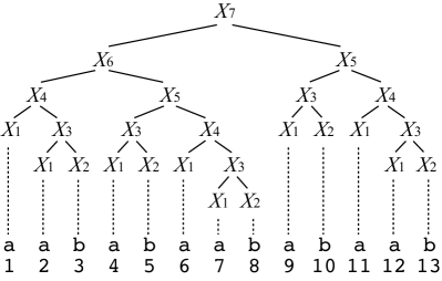
Figure 1: The derivation tree of SLP $\mathcal{T}=\{X_{i}\}_{i=1}^{7}$ with $X_{1}=\mathtt{a}$, $X_{2}=\mathtt{b}$, $X_{3}=X_{1}X_{2}$, $X_{4}=X_{1}X_{3}$, $X_{5}=X_{3}X_{4}$, $X_{6}=X_{4}X_{5}$, and $X_{7}=X_{6}X_{5}$, representing string $T=\mathit{val}(X_{7})=\mathtt{aababaababaab}$.

A straight line program (SLP) $\mathcal{T}$ is a sequence of assignments $X_{1}=expr_{1},X_{2}=expr_{2},\ldots,X_{n}=expr_{n}$, where each $X_{i}$ is a variable and each $expr_{i}$ is an expression, where $expr_{i}=a$ ($a\in\Sigma$), or $expr_{i}=X_{\ell}X_{r}$ ($\ell,r<i$). Let $\mathit{val}(X_{i})$ represent the string derived from $X_{i}$. When it is not confusing, we identify a variable $X_{i}$ with $\mathit{val}(X_{i})$. Then, $|X_{i}|$ denotes the length of the string $X_{i}$ derives. An SLP $\mathcal{T}$ represents the string $T=\mathit{val}(X_{n})$. The size of the program $\mathcal{T}$ is the number $n$ of assignments in $\mathcal{T}$. (See Fig. 1)

The substring intervals of $T$ that each variable derives can be defined recursively as follows: $\mathit{itv}(X_{n})=\{[1:|T|]\}$, and $\mathit{itv}(X_{i})=\{[u+|X_{\ell}|:v]\mid X_{k}=X_{\ell}X_{i},[u:v]\in\mathit{itv}(X_{k})\}\cup\{[u:u+|X_{i}|-1]\mid X_{k}=X_{i}X_{r},[u:v]\in\mathit{itv}(X_{k})\}$ for $i<n$. For example, $\mathit{itv}(X_{5})=\{[4:8],[9:13]\}$ in Fig. 1. Considering the transitive reduction of set inclusion, the intervals $\cup_{i=1}^{n}\mathit{itv}(X_{i})$ naturally form a binary tree (the derivation tree). Let $\mathit{vOcc}(X_{i})=|\mathit{itv}(X_{i})|$ denote the number of times a variable $X_{i}$ occurs in the derivation of $T$. $\mathit{vOcc}(X_{i})$ for all $1\leq i\leq n$ can be computed in $O(n)$ time by a simple iteration on the variables, since $\mathit{vOcc}(X_{n})=1$ and for $i<n$, $\mathit{vOcc}(X_{i})=\sum\{\mathit{vOcc}(X_{k})\mid X_{k}=X_{\ell}X_{i}\}+\sum\{\mathit{vOcc}(X_{k})\mid X_{k}=X_{i}X_{r}\}$. (See Algorithm 1)

2.2 Suffix Arrays and LCP Arrays

The suffix array $\mathit{SA}$ [18] of any string $T$ is an array of length $|T|$ such that $\mathit{SA}[i]=j$, where $T[j:|T|]$ is the $i$-th lexicographically smallest suffix of $T$. The lcp array of any string $T$ is an array of length $|T|$ such that $\mathit{LCP}[i]$ is the length of the longest common prefix of $T[\mathit{SA}[i-1]:|T|]$ and $T[\mathit{SA}[i]:|T|]$ for $2\leq i\leq|T|$, and $\mathit{LCP}[1]=0$. The suffix array for any string of length $|T|$ can be constructed in $O(|T|)$ time (e.g. [11]) assuming an integer alphabet. Given the text and suffix array, the lcp array can also be calculated in $O(|T|)$ time [13].

3 Algorithm

3.1 Computing $q$-gram Frequencies on Uncompressed Strings

We describe two algorithms (Algorithm 2 and Algorithm 3) for computing the $q$-gram frequencies of a given uncompressed string $T$.

A naïve algorithm for computing the $q$-gram frequencies is given in Algorithm 2. The algorithm constructs an associative array, where keys consist of $q$-grams, and the values correspond to the occurrence frequencies of the $q$-grams. The time complexity depends on the implementation of the associative array, but requires at least $O(q|T|)$ time since each $q$-gram is considered explicitly, and the associative array is accessed $O(|T|)$ times: e.g. $O(q|T|\log|\Sigma|)$ time and $O(q|T|)$ space using a simple trie.

Input: string $T$, integer $q\geq 1$

Report: $(P,|\mathit{Occ}(T,P)|)$ for all $P\in\Sigma^{q}$ where $\mathit{Occ}(T,P)\neq\emptyset$.

$\mathbf{S}\leftarrow\emptyset$;

 // empty associative array

1 for $i\leftarrow 1$ to $|T|-q+1$ do

2       $\mathit{qgram}\leftarrow T[i:i+q-1]$;

3       if $\mathit{qgram}\in\mathrm{keys}(\mathbf{S})$ then $\mathbf{S}[\mathit{qgram}]\leftarrow\mathbf{S}[\mathit{qgram}]+1$;

       else  $\mathbf{S}[\mathit{qgram}]\leftarrow 1$;

       // new $q$-gram

4      

for $\mathit{qgram}\in\mathrm{keys}(\mathbf{S})$ do Report $(\mathit{qgram},\mathbf{S}[\mathit{qgram}])$

Algorithm 2 A naïve algorithm for computing $q$-gram frequencies.

Input: string $T$, integer $q\geq 1$

Report: $(i,|\mathit{Occ}(T,P)|)$ for all $P\in\Sigma^{q}$ and some position $i\in\mathit{Occ}(T,P)$.

1 $\mathit{SA}\leftarrow\mathit{SUFFIXARRAY}(T)$; $\mathit{LCP}\leftarrow\mathit{LCPARRAY}(T,SA)$; $\mathit{count}\leftarrow 1$;

2 for $i\leftarrow 2$ to $|T|+1$ do

3       if $i=|T|+1$ or $\mathit{LCP}[i]<q$ then

4             if $\mathit{count}>0$ then Report $(\mathit{SA}[i-1],\mathit{count})$; $\mathit{count}\leftarrow 0$;

5            

6       if $i\leq|T|$ and $\mathit{SA}[i]\leq|T|-q+1$ then $\mathit{count}\leftarrow\mathit{count}+1$;

7      

Algorithm 3 A linear time algorithm for computing $q$-gram frequencies.

The $q$-gram frequencies of string $T$ can be calculated in $O(|T|)$ time using suffix array $\mathit{SA}$ and lcp array $\mathit{LCP}$, as shown in Algorithm 3. For each $1\leq i\leq|T|$, the suffix $\mathit{SA}[i]$ represents an occurrence of $q$-gram $T[\mathit{SA}[i]:\mathit{SA}[i]+q-1]$, if the suffix is long enough, i.e. $\mathit{SA}[i]\leq|T|-q+1$. The key is that since the suffixes are lexicographically sorted, intervals on the suffix array where the values in the lcp array are at least $q$ represent occurrences of the same $q$-gram. The algorithm runs in $O(|T|)$ time, since $\mathit{SA}$ and $\mathit{LCP}$ can be constructed in $O(|T|)$. The rest is a simple $O(|T|)$ loop. A technicality is that we encode the output for a $q$-gram as one of the positions in the text where the $q$-gram occurs, rather than the $q$-gram itself. This is because there can be a total of $O(|T|)$ different $q$-grams, and if we output them as length-$q$ strings, it would require at least $O(q|T|)$ time.

3.2 Computing $q$-gram Frequencies on SLP

We now describe the core idea of our algorithms, and explain two variations which utilize variants of the two algorithms for uncompressed strings presented in Section 3.1. For $q=1$, the $1$-gram frequencies are simply the frequencies of the alphabet and the output is $(a,\sum\{\mathit{vOcc}(X_{i})\mid X_{i}=a\})$ for each $a\in\Sigma$, which takes only $O(n)$ time. For $q\geq 2$, we make use of Lemma 1 below. The idea is similar to the $mk$ Lemma [5], but the statement is more specific.

Lemma 1

Let $\mathcal{T}=\{X_{i}\}_{i=1}^{n}$ be an SLP that represents string $T$. For an interval $[u:v]$ $(1\leq u<v\leq|T|)$, there exists exactly one variable $X_{i}=X_{\ell}X_{r}$ such that for some $[u^{\prime}:v^{\prime}]\in\mathit{itv}(X_{i})$, the following holds: $[u:v]\subseteq[u^{\prime}:v^{\prime}]$, $u\in[u^{\prime}:u^{\prime}+|X_{\ell}|-1]\in\mathit{itv}(X_{\ell})$ and $v\in[u^{\prime}+|X_{\ell}|:v^{\prime}]\in\mathit{itv}(X_{r})$.

Proof

Consider length $1$ intervals $[u:u]$ and $[v:v]$ corresponding to leaves in the derivation tree. $X_{i}$ corresponds to the lowest common ancestor of these intervals in the derivation tree. ∎

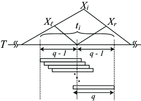
Figure 2: Length-$q$ intervals corresponding to $X_{i}=X_{\ell}X_{r}$.

From Lemma 1, each occurrence of a $q$-gram ($q\geq 2$) represented by some length-$q$ interval of $T$, corresponds to a single variable $X_{i}=X_{\ell}X_{r}$, and is split in two by intervals corresponding to $X_{\ell}$ and $X_{r}$. On the other hand, consider all length-$q$ intervals that correspond to a given variable. Counting the frequencies of the $q$-grams they represent, and summing them up for all variables give the frequencies of all $q$-grams of $T$.

For variable $X_{i}=X_{\ell}X_{r}$, let $t_{i}=\mathit{suf}(X_{\ell},q-1)\mathit{pre}(X_{r},q-1)$. Then, all $q$-grams represented by length $q$ intervals that correspond to $X_{i}$ are those in $t_{i}$. (Fig. 2). If we obtain the frequencies of all $q$-grams in $t_{i}$, and then multiply each frequency by $\mathit{vOcc}(X_{i})$, we obtain frequencies for the $q$-grams occurring in all intervals derived by $X_{i}$. It remains to sum up the $q$-gram frequencies of $t_{i}$ for all $1\leq i\leq n$. We can regard it as obtaining the weighted $q$-gram frequencies in the set of strings $\{t_{1},\ldots,t_{n}\}$, where each $q$-gram in $t_{i}$ is weighted by $\mathit{vOcc}(X_{i})$.

We further reduce this problem to a weighted $q$-gram frequency problem for a single string $z$ as in Algorithm 4. String $z$ is constructed by concatenating $t_{i}$ such that $q\leq|t_{i}|\leq 2(q-1)$, and the weights of $q$-grams starting at each position in $z$ is held in array $w$. On line 4, $0$’s instead of $\mathit{vOcc}(X_{i})$ are appended to $w$ for the last $q-1$ values corresponding to $t_{i}$. This is to avoid counting unwanted $q$-grams that are generated by the concatenation of $t_{i}$ to $z$ on line 4, which are not substrings of each $t_{i}$. The weighted $q$-gram frequency problem for a single string (Line 4) can be solved with a slight modification of Algorithm 2 or 3. The modified algorithms are shown respectively in Algorithms 5 and 6.

Theorem 3.1

Given an SLP ${\mathcal{T}}=\{X_{i}\}_{i=1}^{n}$ of size $n$ representing a string $T$, the $q$-gram frequencies of $T$ can be computed in $O(qn)$ time for any $q>0$.

Proof

Consider Algorithm 4. The correctness is straightforward from the above arguments, so we consider the time complexity. Line 4 can be computed in $O(n)$ time. Line 4 can be computed in $O(qn)$ time by a simple dynamic programming. For $\mathit{pre}()$: If $X_{i}=a$ for some $a\in\Sigma$, then $\mathit{pre}(X_{i},q-1)=a$. If $X_{i}=X_{\ell}X_{r}$ and $|X_{\ell}|\geq q-1$, then $\mathit{pre}(X_{i},q-1)=\mathit{pre}(X_{\ell},q-1)$. If $X_{i}=X_{\ell}X_{r}$ and $|X_{\ell}|<q-1$, then $\mathit{pre}(X_{i},q-1)=\mathit{pre}(X_{\ell},q-1)\mathit{pre}(X_{r},q-1-|X_{\ell}|)$. The strings $\mathit{suf}()$ can be computed similarly. The computation amounts to copying $O(q)$ characters for each variable, and thus can be done in $O(qn)$ time. For the loop at line 4, since the length of string $t_{i}$ appended to $z$, as well as the number of elements appended to $w$ is at most $2(q-1)$ in each loop, the total time complexity is $O(qn)$. Finally, since the length of $z$ and $w$ is $O(qn)$, line 4 can be calculated in $O(qn)$ time using the weighted version of Algorithm 3 (Algorithm 6). ∎

Note that the time complexity for using the weighted version of Algorithm 2 for line 4 of Algorithm 4 would be at least $O(q^{2}n)$: e.g. $O(q^{2}n\log|\Sigma|)$ time and $O(q^{2}n)$ space using a trie.

Input: SLP ${\mathcal{T}}=\{X_{i}\}_{i=1}^{n}$ representing string $T$, integer $q\geq 2$.

Report: all $q$-grams and their frequencies which occur in $T$.

1 Calculate $\mathit{vOcc}(X_{i})$ for all $1\leq i\leq n$;

2 Calculate $\mathit{pre}(X_{i},q-1)$ and $\mathit{suf}(X_{i},q-1)$ for all $1\leq i\leq n-1$ ;

3 $z\leftarrow\varepsilon$; $w\leftarrow[]$;

4 for $i\leftarrow 1$ to $n$ do

5       if $X_{i}=X_{\ell}X_{r}$ and $|X_{i}|\geq q$ then

6             $t_{i}=\mathit{suf}(X_{\ell},q-1)\mathit{pre}(X_{r},q-1)$; $z$.append($t_{i}$);

7             for $j\leftarrow 1$ to $|t_{i}|-q+1$ do $w$.append($\mathit{vOcc}(X_{i})$);

8             for $j\leftarrow 1$ to $q-1$ do $w$.append(0);

9            

10      

Report $q$-gram frequencies in $z$, where each $q$-gram $z[i:i+q-1]$ is weighted by $w[i]$.

Algorithm 4 Calculating $q$-gram frequencies of an SLP for $q\geq 2$

Input: string $T$, array of integers $w$ of length $|T|$, integer $q\geq 1$

Report: $(P,\sum_{i\in\mathit{Occ}(T,P)}w[i])$ for all $P\in\Sigma^{q}$ where $\sum_{i\in\mathit{Occ}(T,P)}w[i]>0$.

$\mathbf{S}\leftarrow\emptyset$;

 // empty associative array

1 for $i\leftarrow 1$ to $|T|-q+1$ do

2       $\mathit{qgram}\leftarrow T[i:i+q-1]$;

3       if $\mathit{qgram}\in\mathrm{keys}(\mathbf{S})$ then $\mathbf{S}[\mathit{qgram}]\leftarrow\mathbf{S}[\mathit{qgram}]+w[i]$;

       else if $w[i]>0$ then $\mathbf{S}[\mathit{qgram}]\leftarrow w[i]$;

       // new $q$-gram

4      

for $\mathit{qgram}\in\mathrm{keys}(\mathbf{S})$ do Report $(\mathit{qgram},\mathbf{S}[\mathit{qgram}])$

Algorithm 5 A variant of Algorithm 2 for weighted $q$-gram frequencies.

Input: string $T$, array of integers $w$ of length $|T|$, integer $q\geq 1$

Output: $(i,\sum_{i\in\mathit{Occ}(T,P)}w[i])$ for all $P\in\Sigma^{q}$ where $\sum_{i\in\mathit{Occ}(T,P)}w[i]>0$ and some position $i\in\mathit{Occ}(T,P)$.

1 $\mathit{SA}\leftarrow\mathit{SUFFIXARRAY}(T)$; $\mathit{LCP}\leftarrow\mathit{LCPARRAY}(T,SA)$; $\mathit{count}\leftarrow 1$;

2 for $i\leftarrow 2$ to $|T|+1$ do

3       if $i=|T|+1$ or $\mathit{LCP}[i]<q$ then

4             if $\mathit{count}>0$ then Report $(\mathit{SA}[i-1],\mathit{count})$; $\mathit{count}\leftarrow 0$;

5            

6       if $i\leq|T|$ and $\mathit{SA}[i]\leq|T|-q+1$ then $\mathit{count}\leftarrow\mathit{count}+w[\mathit{SA}[i]]$;

7      

Algorithm 6 A variant of Algorithm 3 for weighted $q$-gram frequencies.

4 Applications and Extensions

We showed that for an SLP ${\mathcal{T}}$ of size $n$ representing string $T$, $q$-gram frequency problems on $T$ can be reduced to weighted $q$-gram frequency problems on a string $z$ of length $O(qn)$, which can be much shorter than $T$. This idea can further be applied to obtain efficient compressed string processing algorithms for interesting problems which we briefly introduce below.

4.1 $q$-gram Spectrum Kernel

A string kernel is a function that computes the inner product between two strings which are mapped to some feature space. It is used when classifying string or text data using methods such as Support Vector Machines (SVMs), and is usually the dominating factor in the time complexity of SVM learning and classification. A $q$-gram spectrum kernel [16] considers the feature space of $q$-grams. For string $T$, let $\phi_{q}(T)=(|\mathit{Occ}(T,p)|)_{p\in\Sigma^{q}}$. The kernel function is defined as $K_{q}(T_{1},T_{2})=\langle\phi_{q}(T_{1}),\phi_{q}(T_{2})\rangle=\sum_{p\in\Sigma^{q}}|\mathit{Occ}(T_{1},p)||\mathit{Occ}(T_{2},p)|$. The calculation of the kernel function amounts to summing up the product of occurrence frequencies in strings $T_{1}$ and $T_{2}$ for all $q$-grams which occur in both $T_{1}$ and $T_{2}$. This can be done in $O(|T_{1}|+|T_{2}|)$ time using suffix arrays. For two SLPs ${\mathcal{T}_{1}}$ and ${\mathcal{T}_{2}}$ of size $n_{1}$ and $n_{2}$ representing strings $T_{1}$ and $T_{2}$, respectively, the $q$-gram spectrum kernel $K_{q}(T_{1},T_{2})$ can be computed in $O(q(n_{1}+n_{2}))$ time by a slight modification of our algorithm.

4.2 Optimal Substring Patterns of Length $q$

Given two sets of strings, finding string patterns that are frequent in one set and not in the other, is an important problem in string data mining, with many problem formulations and the types of patterns to be considered, e.g.: in Bioinformatics [3], Machine Learning (optimal patterns [2]), and more recently KDD (emerging patterns [4]). A simple optimal $q$-gram pattern discovery problem can be defined as follows: Let $\mathbf{T_{1}}$ and $\mathbf{T_{2}}$ be two multisets of strings. The problem is to find the $q$-gram $p$ which gives the highest (or lowest) score according to some scoring function that depends only on $|\mathbf{T_{1}}|$, $|\mathbf{T_{2}}|$, and the number of strings respectively in $\mathbf{T_{1}}$ and $\mathbf{T_{2}}$ for which $p$ is a substring. For uncompressed strings, the problem can be solved in $O(N)$ time, where $N$ is the total length of the strings in both $\mathbf{T_{1}}$ and $\mathbf{T_{2}}$, by applying the algorithm of [9] to two sets of strings. For the SLP compressed version of this problem, the input is two multisets of SLPs, each representing strings in $\mathbf{T_{1}}$ and $\mathbf{T_{2}}$. If $n$ is the total number of variables used in all of the SLPs, the problem can be solved in $O(qn)$ time.

4.3 Different Lengths

The ideas in this paper can be used to consider all substrings of length not only $q$, but all lengths up-to $q$, with some modifications. For the applications discussed above, although the number of such substrings increases to $O(q^{2}n)$, the $O(qn)$ time complexity can be maintained by using standard techniques of suffix arrays [7, 13]. This is because there exist only $O(qn)$ substring with distinct frequencies (corresponding to nodes of the suffix tree), and the computations of the extra substrings can be summarized with respect to them.

5 Computational Experiments

We implemented 4 algorithms (NMP, NSA, SMP, SSA) that count the frequencies of all $q$-grams in a given text. NMP (Algorithm 2) and NSA (Algorithm 3) work on the uncompressed text. SMP (Algorithm 4 + Algorithm 5) and SSA (Algorithm 4 + Algorithm 6) work on SLPs. The algorithms were implemented using the C++ language. We used std::map from the Standard Template Library (STL) for the associative array implementation. For constructing suffix arrays, we used the divsufsort library developed by Yuta Mori. This implementation is not linear time in the worst case, but has been empirically shown to be one of the fastest implementations on various data.

All computations were conducted on a Mac Xserve (Early 2009) with 2 x 2.93GHz Quad Core Xeon processors and 24GB Memory, only utilizing a single process/thread at once. The program was compiled using the GNU C++ compiler (g++) 4.2.1 with the -fast option for optimization. The running times are measured in seconds, starting from after reading the uncompressed text into memory for NMP and NSA, and after reading the SLP that represents the text into memory for SMP and SSA. Each computation is repeated at least 3 times, and the average is taken.

5.1 Fibonacci Strings

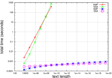
Figure 3: Running times of NMP, NSA, SMP, SSA on Fibonacci strings for $q=50$.

The $i$ th Fibonacci string $F_{i}$ can be represented by the following SLP: $X_{1}=\mathtt{b}$, $X_{2}=\mathtt{a}$, $X_{i}=X_{i-1}X_{i-2}$ for $i>2$, and $F_{i}=\mathit{val}(X_{i})$. Fig. 3 shows the running times on Fibonacci strings $F_{20},F_{25},\ldots,F_{95}$, for $q=50$. Although this is an extreme case since Fibonacci strings can be exponentially compressed, we can see that SMP and SSA that work on the SLP are clearly faster than NMP and NSA which work on the uncompressed string.

5.2 Pizza & Chili Corpus

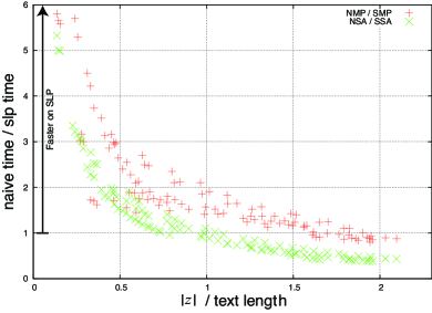
Figure 4: Time ratios NMP/SMP and NSA/SSA plotted against ratio $|z|/|T|$.

We also applied the algorithms on texts XML, DNA, ENGLISH, and PROTEINS, with sizes 50MB, 100MB, and 200MB, obtained from the Pizza & Chili Corpus. We used RE-PAIR [15] to obtain SLPs for this data.

Table 1 shows the running times for all algorithms and data, where $q$ is varied from $2$ to $10$. We see that for all corpora, SMP and SSA running on SLPs are actually faster than NMP and NSA running on uncompressed text, when $q$ is small. Furthermore, SMP is faster than SSA when $q$ is smaller. Interestingly for XML, the SLP versions are faster even for $q$ up to $9$.

Fig. 4 shows the same results as time ratio: NMP/SMP and NSA/ SSA, plotted against ratio: (length of $z$ in Algorithm 4)/(length of uncompressed text). As expected, the SLP versions are basically faster than their uncompressed counterparts, when $|z|/\mbox{(text length)}$ is less than $1$, since the SLP versions run the weighted versions of the uncompressed algorithms on a text of length $|z|$. SLPs generated by other grammar based compression algorithms showed similar tendencies (data not shown).

Table 1: Running times in seconds for data from the Pizza & Chili Corpus. Bold numbers represent the fastest time for each data and $q$. Times for SMP and SSA are prefixed with $\triangleright$, if they become fastest when all algorithms start from the SLP representation, i.e., NMP and NSA require time for decompressing the SLP (denoted by decompression time). The bold horizontal lines show the boundary where $|z|$ in Algorithm 4 exceeds the uncompressed text length.

XML
	50MB					100MB					200MB
	SLP Size:			2,702,383		SLP Size:			5,059,578		SLP Size:			9,541,590
	decompression time:			0.82 secs		decompression time:			1.73 secs		decompression time:			3.52 secs
$q$	$|z|$	NMP	NSA	SMP	SSA	$|z|$	NMP	NSA	SMP	SSA	$|z|$	NMP	NSA	SMP	SSA
2	8,106,861	5.9	9.8	1.1	2.0	15,178,446	12.0	21.0	2.1	4.3	28,624,482	24.7	46.9	4.3	8.9
3	13,413,565	13.0	9.8	2.5	3.2	25,160,162	27.8	21.1	4.9	6.8	47,504,478	58.7	46.1	9.8	14.3
4	18,364,951	21.0	9.8	5.7	4.7	34,581,658	47.2	21.3	11.3	9.9	65,496,619	100.3	46.2	22.5	20.0
5	22,873,060	28.7	9.8	10.2	5.9	43,275,004	63.0	21.1	20.4	12.5	82,321,682	139.4	46.2	40.1	25.1
6	27,032,514	35.2	9.8	14.9	7.1	51,354,178	77.1	21.0	29.6	14.8	98,124,580	172.4	46.3	59.4	30.2
7	30,908,898	40.0	9.8	19.4	8.2	58,935,352	87.4	21.1	38.9	16.9	113,084,186	197.7	46.8	78.5	34.9
8	34,559,523	44.3	9.8	26.0	9.3	66,104,075	97.5	21.1	52.5	19.1	127,316,007	218.3	46.3	103.9	39.9
9	37,983,150	49.0	9.8	31.0	$\triangleright$ 10.1	72,859,310	105.3	21.1	60.9	20.9	140,846,749	234.6	46.3	124.7	44.1
10	41,253,257	52.5	9.9	35.8	11.2	79,300,797	115.3	21.2	72.2	$\triangleright$ 22.7	153,806,891	253.6	46.3	148.8	$\triangleright$ 48.8
DNA
	50MB					100MB					200MB
	SLP Size:			6,406,324		SLP Size:			12,233,978		SLP Size:			23,171,463
	decompression time:			1.23 secs		decompression time:			2.54 secs		decompression time:			5.21 secs
$q$	$|z|$	NMP	NSA	SMP	SSA	$|z|$	NMP	NSA	SMP	SSA	$|z|$	NMP	NSA	SMP	SSA
2	19,218,924	2.2	13.7	1.9	5.7	36,701,886	4.7	30.5	3.9	12.6	69,514,341	9.8	70.0	8.0	26.1
3	32,030,826	4.4	13.7	3.0	8.6	61,169,030	9.1	30.5	5.8	18.6	115,856,038	18.7	70.1	11.8	38.8
4	44,833,624	6.5	13.7	4.5	12.3	85,624,856	13.4	30.5	8.9	25.3	162,182,697	28.0	70.0	17.6	52.9
5	57,554,843	8.6	13.8	6.7	15.5	109,976,706	17.8	30.5	13.1	32.3	208,371,656	37.0	69.9	26.3	67.9
6	69,972,618	11.1	13.7	10.1	19.0	133,890,719	23.3	31.0	19.8	40.0	253,939,731	47.6	70.2	39.5	86.6
7	81,771,222	15.3	13.6	$\triangleright$ 14.7	23.0	156,832,841	31.0	30.5	28.6	49.3	298,014,802	63.2	69.9	56.1	104.5
8	92,457,893	21.1	13.6	22.9	27.3	177,888,984	42.2	30.5	44.9	58.5	338,976,517	85.4	69.9	88.5	126.3
9	101,852,490	33.0	13.7	42.8	31.4	196,656,282	65.7	30.4	81.5	67.5	375,928,060	132.1	69.9	159.3	147.9
10	109,902,230	56.5	13.7	65.9	34.9	213,075,531	113.2	30.5	129.2	75.9	408,728,193	226.0	69.9	248.4	166.3
ENGLISH
	50MB					100MB					200MB
	SLP Size:			4,861,619		SLP Size:			10,063,953		SLP Size:			18,945,126
	decompression time:			1.15 secs		decompression time:			2.43 secs		decompression time:			5.07 secs
$q$	$|z|$	NMP	NSA	SMP	SSA	$|z|$	NMP	NSA	SMP	SSA	$|z|$	NMP	NSA	SMP	SSA
2	14,584,329	5.7	13.1	1.9	4.5	30,191,214	11.5	28.2	4.2	10.3	56,834,703	23.5	64.2	8.5	21.7
3	24,230,676	11.4	13.0	4.0	7.4	50,196,054	23.8	28.2	8.3	16.8	94,552,062	50.3	65.5	16.5	34.9
4	33,655,433	20.0	12.9	8.2	9.9	69,835,185	42.1	28.2	17.6	22.1	131,758,513	89.7	64.2	34.1	45.8
5	42,640,982	33.1	12.9	16.1	12.7	88,711,756	72.6	28.2	35.1	$\triangleright$ 28.6	167,814,701	156.9	64.2	68.2	59.7
6	51,061,064	49.5	12.9	27.1	15.5	106,583,131	111.8	28.5	59.7	35.3	202,293,814	240.8	64.4	116.1	74.3
7	58,791,311	65.1	12.9	40.1	18.4	123,180,654	143.6	28.3	88.3	42.3	234,664,404	313.7	64.3	173.5	90.3
8	65,777,414	79.6	12.9	59.1	20.8	138,382,443	176.8	28.3	131.3	48.5	264,668,656	385.9	64.8	256.7	104.5
9	71,930,623	92.7	12.9	74.2	23.0	152,010,306	207.8	28.5	166.0	54.2	291,964,684	454.6	64.5	335.0	118.0
10	77,261,995	105.3	13.0	89.7	25.1	164,021,382	235.9	28.4	205.2	59.8	316,387,791	521.2	64.7	425.3	131.4
PROTEINS
	50MB					100MB					200MB
	SLP Size:			10,357,053		SLP Size:			18,806,316		SLP Size:			32,375,988
	decompression time:			1.67 secs		decompression time:			3.51 secs		decompression time:			7.05 secs
$q$	$|z|$	NMP	NSA	SMP	SSA	$|z|$	NMP	NSA	SMP	SSA	$|z|$	NMP	NSA	SMP	SSA
2	31,071,084	4.5	14.5	4.0	10.2	56,418,873	9.0	32.2	7.6	20.4	97,127,889	18.0	69.0	13.6	38.0
3	51,749,628	9.4	14.5	7.6	16.2	93,995,974	18.7	32.1	14.1	32.3	161,825,337	37.3	69.0	25.5	60.0
4	70,939,655	22.4	14.3	21.3	24.6	129,372,571	45.4	32.2	39.1	49.0	223,413,554	91.5	69.0	$\triangleright$ 69.1	91.8
5	86,522,157	66.6	14.4	54.9	32.2	159,110,124	137.5	32.2	100.5	65.6	275,952,088	270.9	69.4	175.5	125.1
6	95,684,819	116.7	14.5	107.7	37.6	178,252,162	251.5	32.3	204.4	79.1	311,732,866	502.8	69.4	356.0	151.7
7	99,727,910	142.8	14.5	143.7	40.8	187,623,783	327.6	32.4	299.8	85.6	330,860,933	675.2	69.7	586.4	168.0
8	100,877,101	147.8	14.4	166.3	42.5	190,898,844	343.0	32.4	363.6	88.7	337,898,827	731.0	69.6	771.8	175.5
9	101,631,544	149.3	14.4	171.6	42.8	192,736,305	348.1	32.4	393.0	91.2	341,831,651	742.2	69.7	820.3	181.8
10	102,636,144	150.5	14.4	178.6	43.4	195,044,390	350.4	32.5	404.2	93.1	346,403,103	747.7	69.7	831.9	185.8

6 Conclusion

We presented an $O(qn)$ time and space algorithm for calculating all $q$-gram frequencies in a string, given an SLP of size $n$ representing the string. This solves, much more efficiently, a more general problem than considered in previous work. Computational experiments on various real texts showed that the algorithms run faster than algorithms that work on the uncompressed string, when $q$ is small. Although larger values of $q$ allow us to capture longer character dependencies, the dimensionality of the features increases, making the space of occurring $q$-grams sparse. Therefore, meaningful values of $q$ for typical applications can be fairly small in practice (e.g. $3\sim 6$), so our algorithms have practical value.

A future work is extending our algorithms that work on SLPs, to algorithms that work on collage systems [14]. A Collage System is a more general framework for modeling various compression methods. In addition to the simple concatenation operation used in SLPs, it includes operations for repetition and prefix/suffix truncation of variables.

This is the first paper to show the potential of the compressed string processing approach in developing efficient and practical algorithms for problems in the field of string mining and classification. More and more efficient algorithms for various processing of text in compressed representations are becoming available. We believe texts will eventually be stored in compressed form by default, since not only will it save space, but it will also have the added benefit of being able to conduct various computations on it more efficiently later on, when needed.

References

- [1] Amir, A., Benson, G.: Efficient two-dimensional compressed matching. In: Proc. Data Compression Conference 1992 (DCC ’92). pp. 279–288 (1992)
- [2] Arimura, H., Wataki, A., Fujino, R., Arikawa, S.: A fast algorithm for discovering optimal string patterns in large text databases. In: Proc. 9th International Conference on Algorithmic Learning Theory (ALT ’98). pp. 247–261 (1998)
- [3] Brazma, A., Jonassen, I., Eidhammer, I., Gilbert, D.: Approaches to the automatic discovery of patterns in biosequences. J. Comp. Biol. 5(2), 279–305 (1998)
- [4] Chan, S., Kao, B., Yip, C.L., Tang, M.: Mining emerging substrings. In: Proc. 8th International Conference on Database Systems for Advanced Applications (DASFAA ’03). p. 119 (2003)
- [5] Charikar, M., Lehman, E., Liu, D., Panigrahy, R., Prabhakaran, M., Sahai, A., abhi shelat: The smallest grammar problem. IEEE Transactions on Information Theory 51(7), 2554–2576 (2005)
- [6] Claude, F., Navarro, G.: Self-indexed grammar-based compression. Fundamenta Informaticae (to appear), preliminary version: Proc. MFCS 2009 pp. 235–246
- [7] Gusfield, D.: Algorithms on Strings, Trees, and Sequences. Cambridge University Press (1997)
- [8] Hermelin, D., Landau, G.M., Landau, S., Weimann, O.: A unified algorithm for accelerating edit-distance computation via text-compression. In: Proc. STACS 2009. pp. 529–540 (2009)
- [9] Hui, L.C.K.: Color set size problem with application to string matching. In: Proc. CPM 1992. LNCS, vol. 644, pp. 230–243 (1992)
- [10] Inenaga, S., Bannai, H.: Finding characteristic substring from compressed texts. In: Proc. The Prague Stringology Conference 2009. pp. 40–54 (2009)
- [11] Kärkkäinen, J., Sanders, P.: Simple linear work suffix array construction. In: Proc. ICALP 2003. LNCS, vol. 2719, pp. 943–955 (2003)
- [12] Karpinski, M., Rytter, W., Shinohara, A.: An efficient pattern-matching algorithm for strings with short descriptions. Nordic Journal of Computing 4, 172–186 (1997)
- [13] Kasai, T., Lee, G., Arimura, H., Arikawa, S., Park, K.: Linear-time Longest-Common-Prefix Computation in Suffix Arrays and Its Applications. In: Proc. CPM 2001. LNCS, vol. 2089, pp. 181–192 (2001)
- [14] Kida, T., Shibata, Y., Takeda, M., Shinohara, A., Arikawa, S.: Collage system: A unifying framework for compressed pattern matching. Theoret. Comput. Sci. 298, 253–272 (2003)
- [15] Larsson, N.J., Moffat, A.: Offline dictionary-based compression. In: Proc. Data Compression Conference 1999 (DCC ’99). pp. 296–305 (1999)
- [16] Leslie, C., Eskin, E., Noble, W.S.: The spectrum kernel: A string kernel for SVM protein classification. In: Pacific Symposium on Biocomputing. vol. 7, pp. 566–575 (2002)
- [17] Lifshits, Y.: Processing compressed texts: A tractability border. In: Proc. CPM 2007. LNCS, vol. 4580, pp. 228–240 (2007)
- [18] Manber, U., Myers, G.: Suffix arrays: A new method for on-line string searches. SIAM J. Computing 22(5), 935–948 (1993)
- [19] Matsubara, W., Inenaga, S., Ishino, A., Shinohara, A., Nakamura, T., Hashimoto, K.: Efficient algorithms to compute compressed longest common substrings and compressed palindromes. Theoret. Comput. Sci. 410(8–10), 900–913 (2009)
- [20] Navarro, G., Mäkinen, V.: Compressed full-text indexes. ACM Computing Surveys 39(1), 2 (2007)
- [21] Nevill-Manning, C.G., Witten, I.H., Maulsby, D.L.: Compression by induction of hierarchical grammars. In: Proc. Data Compression Conference 1994 (DCC ’94). pp. 244–253 (1994)
- [22] Rytter, W.: Application of Lempel-Ziv factorization to the approximation of grammar-based compression. Theoret. Comput. Sci. 302(1–3), 211–222 (2003)
- [23] Shibata, Y., Kida, T., Fukamachi, S., Takeda, M., Shinohara, A., Shinohara, T., Arikawa, S.: Speeding up pattern matching by text compression. In: Proc. 4th Italian Conference on Algorithms and Complexity (CIAC 2000). LNCS, vol. 1767, pp. 306–315 (2000)
- [24] Ziv, J., Lempel, A.: A universal algorithm for sequential data compression. IEEE Transactions on Information Theory IT-23(3), 337–349 (1977)
- [25] Ziv, J., Lempel, A.: Compression of individual sequences via variable-length coding. IEEE Transactions on Information Theory 24(5), 530–536 (1978)