Equatorial Superrotation on tidally locked exoplanets

Abstract

The increasing richness of exoplanet observations has motivated a variety of three-dimensional atmospheric circulation models of these planets. Under strongly irradiated conditions, models of tidally locked, short-period planets (both hot Jupiters and terrestrial planets) tend to exhibit a circulation dominated by a fast eastward, or “superrotating,” jet stream at the equator. When the radiative and advection time scales are comparable, this phenomenon can cause the hottest regions to be displaced eastward from the substellar point by tens of degrees longitude. Such an offset has been subsequently observed on HD 189733b, supporting the possibility of equatorial jets on short-period exoplanets. Despite its relevance, however, the dynamical mechanisms responsible for generating the equatorial superrotation in such models have not been identified. Here, we show that the equatorial jet results from the interaction of the mean flow with standing Rossby waves induced by the day-night thermal forcing. The strong longitudinal variations in radiative heating—namely intense dayside heating and nightside cooling—trigger the formation of standing, planetary-scale equatorial Rossby and Kelvin waves. The Rossby waves develop phase tilts that pump eastward momentum from high latitudes to the equator, thereby inducing equatorial superrotation. We present an analytic theory demonstrating this mechanism and explore its properties in a hierarchy of one-layer (shallow-water) calculations and fully 3D models. The wave-mean-flow interaction produces an equatorial jet whose latitudinal width is comparable to that of the Rossby waves, namely the equatorial Rossby deformation radius modified by radiative and frictional effects. For conditions typical of synchronously rotating hot Jupiters, this length is comparable to a planetary radius, explaining the broad scale of the equatorial jet obtained in most hot Jupiter models. Our theory illuminates the dependence of the equatorial jet speed on forcing amplitude, strength of friction, and other parameters, as well as the conditions under which jets can form at all.

1. Introduction

The past few years have witnessed major strides in our efforts to understand the atmospheric circulation of short-period exoplanets—both gas giants (hot Jupiters) and smaller terrestrial planets. Infrared photometry, spectra, and light curves from the Spitzer and Hubble Space Telescopes now provide constraints on the three-dimensional temperature structure of several hot Jupiters, which hint at a vigorous atmospheric circulation on these bodies (e.g., Knutson et al., 2007, 2009; Charbonneau et al., 2008; Harrington et al., 2006; Cowan et al., 2007; Swain et al., 2009; Crossfield et al., 2010). These observations have motivated a growing effort to model the atmospheric circulation on these objects: to date, many three-dimensional atmospheric circulation models of hot Jupiters have been published (Showman & Guillot, 2002; Cooper & Showman, 2005, 2006; Showman et al., 2008, 2009; Dobbs-Dixon & Lin, 2008; Menou & Rauscher, 2009; Rauscher & Menou, 2010; Dobbs-Dixon et al., 2010; Thrastarson & Cho, 2010; Lewis et al., 2010; Perna et al., 2010; Heng et al., 2010). These models have emphasized synchronously rotating hot Jupiters in circular, approximately 2–5-day orbits.

Just as the last decade witnessed the first characterization of hot Jupiters, the next decade will see a shift toward characterizing “super Earths” (planets of 1–10 Earth masses) and terrestrial planets. To date, roughly 30 super Earths have been discovered, including several that transit their host stars (Charbonneau et al., 2009; Léger et al., 2009; Batalha et al., 2011) with hundreds of additional candidates recently announced from the NASA Kepler mission (Borucki et al., 2011). Attempts to observationally characterize their atmospheres have already begun (Bean et al., 2010). In anticipation of this vanguard, several three-dimensional circulation models of tidally locked, short-period terrestrial exoplanets have been published (Joshi et al., 1997; Joshi, 2003; Merlis & Schneider, 2010; Heng & Vogt, 2010).

Intriguingly, the flows in most of these three-dimensional models—both hot Jupiters and terrestrial planets—develop a fast eastward, or superrotating, jet stream at the equator, with westward flow typically occurring at deeper levels and/or higher latitudes. In hot-Jupiter models, the superrotating jet extends from the equator to latitudes of typically 20–$60^{\circ}$ and is perhaps the dominant dynamical feature of the modeled flows. In some cases (depending on the strength of the imposed stellar heating and other factors), this jet causes an eastward displacement of the hottest regions from the substellar point by $\sim$$10^{\circ}$ to $60^{\circ}$ longitude. Showman & Guillot (2002) first predicted this feature and suggested that, if it existed on hot Jupiters, it would have important implications for infrared spectra and light curves. This prediction has been confirmed in Spitzer infrared observations of HD 189733b (Knutson et al., 2007, 2009), suggesting that this planet may indeed exhibit a superrotating jet.

However, despite the ubiquity of equatorial superrotation in three-dimensional models of synchronously rotating exoplanets—and its relevance for observations—the mechanisms that produce this superrotation have yet to be identified. As demonstrated in a theorem due to Hide (1969), such superrotation cannot result from atmospheric circulations that are longitudinally symmetric or that conserve angular momentum per mass about the planetary rotation axis. The equatorial atmosphere is the region of the planet farthest from the planetary rotation axis, and a superrotating equatorial jet therefore corresponds to a local maximum in the angular momentum per mass about the planetary rotation axis. Thus, any angular-momentum-conserving circulation that moves air to the equatorial atmosphere from higher latitudes or deeper levels tends to produce westward equatorial flow. Equivalently, Coriolis forces always induce westward acceleration for air moving equatorward or upward, so an eastward equatorial jet cannot result from Coriolis forces acting on air that moves into the equatorial atmosphere from higher latitudes or deeper levels. In Earth’s equatorial troposphere, for example, the flow is westward, which results from the tropospheric Hadley cell on Earth (a regime where a mean overturning circulation and its Coriolis accelerations plays the defining role (Held & Hou, 1980)). To maintain equatorial superrotation, a mechanism is needed that pumps angular momentum per mass from regions where it is small (outside the jet) to regions where it is large (within the jet)—a so-called “up-gradient” momentum transport. According to Hide’s theorem, this transport can only be accomplished by waves or eddies.

Equatorial superrotation exists in several atmospheres of the Solar System—the equatorial atmospheres of Venus, Titan, Jupiter, and Saturn all superrotate. Even localized layers within Earth’s equatorial stratosphere exhibit superrotation, part of a phenomenon called the “Quasi-Biennial Oscillation” or QBO (Andrews et al., 1987). The mechanisms for driving the equatorial superrotation on these planets are diverse. Possible mechanisms include eddy transport associated with baroclinic instabilities, barotropic instabilities, turbulence, and the absorption/radiation of various types of atmospheric waves (e.g., Williams, 2003b, a; Lian & Showman, 2008, 2010; Schneider & Liu, 2009; Del Genio et al., 1993; Del Genio & Zhou, 1996; Andrews et al., 1987; Mitchell & Vallis, 2010).

Here, we demonstrate how the equatorial superrotation in three-dimensional models of synchronously rotating, short-period exoplanets can result from the existence of standing, planetary-scale Rossby waves; such waves are naturally excited by the longitudinally dependent heating patterns—dayside heating and nightside cooling—that accompany the photospheric regions of short-period, synchronously rotating planets. Section 2 provides background. In Section 3, we present an analytic theory demonstrating the mechanism, and we systematically explore its behavior in idealized, nonlinear one-layer models. In Section 4 we extend the analysis to three-dimensional circulation models. In Section 5, we summarize and discuss implications.

2. Background Theory

The ability of Rossby waves to accelerate jets can be schematically illustrated using the two-dimensional non-divergent barotropic vorticity equation, which is the simplest model for the global-scale flow of a planetary atmosphere (see discussion in Vallis, 2006; Showman et al., 2010). The equation reads

$${d(\zeta+f)\over dt}=F$$ (1)

where $\zeta\equiv{\bf k}\cdot\nabla\times{\bf v}$ is the relative vorticity, ${\bf v}$ is the horizontal wind velocity, ${\bf k}$ is the local upward unit vector, $f\equiv 2\Omega\sin\phi$ is the Coriolis parameter, $\Omega$ is the planetary rotation rate ($2\pi$ over the rotation period), $\phi$ is latitude, and $d/dt=\partial/\partial t+{\bf v}\cdot\nabla$ is the material derivative (i.e., the derivative following the flow). The equation states that individual fluid parcels conserve the absolute vorticity, $\zeta+f$, save for vorticity sources/sinks, which are represented by the term $F$. The equation can equivalently be written

$${\partial\zeta\over\partial t}+{\bf v}\cdot\nabla\zeta+v\beta=F$$ (2)

where $v$ is the meridional (northward) wind speed and $\beta=df/dy$ is the gradient of the Coriolis parameter with northward distance $y$. Because the flow in this simple model is horizontally non-divergent, we can define a streamfunction $\psi$ such that $u=-\partial\psi/\partial y$ and $v=\partial\psi/\partial x$, where $x$ is the eastward coordinate and $u$ is the zonal (eastward) wind speed. This allows the equation to be written as a function of one variable, $\psi$.

For purposes of illustration, consider the linearized version of Eq. (2) with no sources and sinks. The solutions to this linearized, unforced equation are Rossby waves. For simplicity, we consider Cartesian geometry with constant $\beta$, representing a local region on the sphere. Decomposing variables into zonal means (denoted with overbars) and deviations therefrom (denoted with primes), and assuming that the mean flow is zero, leads to a solution given by $\psi^{\prime}=\hat{\psi}\exp[i(kx+ly)]$, where $i$ is the imaginary number and $k$ and $l$ are the zonal and meridional wavenumbers. The dispersion relation is

$$\omega=-{\beta k\over k^{2}+l^{2}}.$$ (3)

These waves propagate meridionally with a group velocity given by

$${\partial\omega\over\partial l}={2\beta kl\over(k^{2}+l^{2})^{2}}.$$ (4)

A simple argument, first clearly presented by Thompson (1971) and reviewed in Held (2000) and Vallis (2006), shows how these waves can produce an east-west acceleration of the zonal-mean flow. The latitudinal transport of eastward eddy momentum per mass is $\overline{u^{\prime}v^{\prime}}$, where $u^{\prime}$ and $v^{\prime}$ are the deviations of the zonal and meridional winds from their zonal means, respectively, and the overbar denotes a zonal average. Using the solutions for the wave-induced zonal and meridional wind, $u^{\prime}=-il\hat{\psi}\exp[i(kx+ly)]$ and $v^{\prime}=ik\hat{\psi}\exp[i(kx+ly)]$, yields a momentum flux

$$\overline{u^{\prime}v^{\prime}}=-{1\over 2}\hat{\psi}^{2}kl.$$ (5)

Since the group velocity must point away from the region of wave generation (which we call the “wave source”), and since $\beta$ is positive, we must have $kl>0$ north of the source and $kl<0$ south of the source. Thus, north of the source, $\overline{u^{\prime}v^{\prime}}$ is negative, implying southward transport of eastward momentum. But south of the source, $\overline{u^{\prime}v^{\prime}}$ is positive, implying northward transport of eastward momentum. Rossby waves therefore transport eastward momentum into the wave source region. An eastward acceleration must therefore occur in the wave source region and a westward acceleration must occur in the region of wave breaking or dissipation. This can lead to the formation of zonal (east-west) jet streams.

Rossby waves correspond to latitudinal oscillations in surfaces of constant potential vorticity; thus, any process that triggers such oscillations at large scales will tend to excite Rossby waves. In Earth’s atmosphere, one of the predominant sources is baroclinic instability, which occurs in the mid-latitude troposphere where latitudinal temperature gradients are large. Spatially varying tropospheric heating and cooling (e.g., due to land-sea contrasts) or flow over topography also perturb the potential vorticity contours and can therefore trigger Rossby waves. In the atmospheres of tidally locked, hot exoplanets, on the other hand, the day-night heating pattern constitutes the overriding dynamical forcing. For such planets, we expect this heating/cooling pattern to trigger Rossby waves at low latitudes (Fig. 1).

The above theory is for free waves. Consider now the extension to an atmosphere forced by vorticity sources/sinks and damped by frictional drag. The zonal-mean zonal momentum equation of the barotropic system reads

$${\partial\overline{u}\over\partial t}=-{\partial(\overline{u^{\prime}v^{\prime}})\over\partial y}-{\overline{u}\over\tau_{\rm drag}}$$ (6)

where overbars denote zonal means and primes denote deviations therefrom. The equation states that accelerations of the zonal-mean zonal flow result from convergences of the latitudinal eddy momentum flux and from drag, which we have parameterized as a term that relaxes the zonal-mean zonal wind toward zero over a drag time constant $\tau_{\rm drag}$. The relationship between the eddy acceleration in Eq. (6) and the vorticity sources/sinks can be made in two steps. First, we note that the definition of vorticity implies that $\overline{v^{\prime}\zeta^{\prime}}=-\partial(\overline{u^{\prime}v^{\prime}})/\partial y$. Second, we multiply the linearized version of Eq. (2) by $\zeta^{\prime}$ and zonally average. This leads to an equation for the budget of the so-called “pseudomomentum” (Vallis, 2006, p. 493):

$${\partial{\cal A}\over\partial t}+\overline{v^{\prime}\zeta^{\prime}}={\overline{\zeta^{\prime}F^{\prime}}\over 2(\beta-{\partial^{2}\overline{u}\over\partial y^{2}})}.$$ (7)

For the two-dimensional non-divergent model, ${\cal A}=(\beta-\partial^{2}\overline{u}/\partial y^{2})^{-1}\overline{\zeta^{\prime 2}}/2$ is the pseudomomentum, which is a measure of wave activity. By combining Eqs. (6)–(7) and supposing that the wave amplitudes and zonal-mean zonal wind are statistically steady, i.e., $\partial{\cal A}/\partial t\approx 0$ and $\partial\overline{u}/\partial t\approx 0$, we obtain

$${\overline{u}\over\tau_{\rm drag}}={\overline{\zeta^{\prime}F^{\prime}}\over 2(\beta-{\partial^{2}\overline{u}\over\partial y^{2}})}.$$ (8)

This equation relates the vorticity sources/sinks and drag to the zonal-mean zonal wind, $\overline{u}$. When eddy sources/sinks of relative vorticity on average exhibit the same sign as the vorticity itself (i.e. $\overline{\zeta^{\prime}F^{\prime}}>0$), the eddy acceleration is eastward, and in steady state results in an eastward zonal-mean zonal wind. When sources/sink of relative vorticity tend to exhibit the opposite sign as the vorticity ($\overline{\zeta^{\prime}F^{\prime}}<0$), the eddy acceleration is westward, and in steady state results in westward zonal-mean zonal wind. In analogy with the free solutions, this behavior is typically interpreted in terms of the generation, latitudinal propagation, and dissipation of Rossby waves.

This mechanism is thought to be responsible for the eddy-driven jet streams (and the associated eastward surface winds) in Earth’s midlatitudes: baroclinic instability generates Rossby waves that radiate away from the midlatitudes, causing eastward eddy acceleration there and leading to eastward surface flow in steady state (Held, 2000; Vallis, 2006). At the equator, Earth’s troposphere does not superrotate; nevertheless, idealized Earth general circulation models (GCMs) have shown that the presence of strong zonally varying heating and cooling in the tropics can cause equatorial superrotation to emerge (Suarez & Duffy, 1992; Saravanan, 1993; Kraucunas & Hartmann, 2005; Norton, 2006). In analogy with the theory described above, Held (1999) suggested heuristically that the superrotation in these models results from the generation and poleward propagation of Rossby waves by the tropical heating sources.

Still, application of this barotropic theory to tidally locked exoplanets is problematic. Most models of atmospheric circulation on synchronously rotating, zero-eccentricity hot Jupiters exhibit relatively steady circulation patterns whose velocity and temperature patterns are approximately symmetric about the equator (Showman & Guillot, 2002; Cooper & Showman, 2005, 2006; Showman et al., 2008, 2009; Dobbs-Dixon & Lin, 2008; Rauscher & Menou, 2010). In such models, the relative vorticity is approximately antisymmetric about, and zero at, the equator. Eq. (8) predicts that $\overline{u}=0$ at the equator for this situation. Thus, while attractive, this theory fails to explain the equatorial superrotation in these hot Jupiter models.

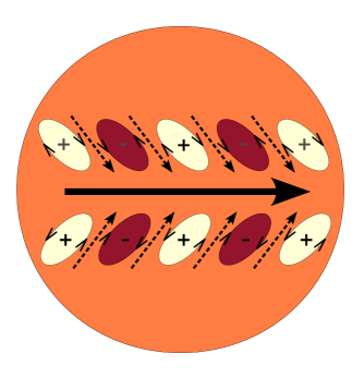
Figure 1.— Illustration of the dynamical mechanism for generating equatorial superrotation on tidally locked short-period exoplanets, including hot Jupiters and super Earths. The intense day-night heating gradient generates standing, planetary-scale Rossby and Kelvin waves. These waves develop a structure with velocities tilting northwest-to-southeast in the northern hemisphere and southwest-to-northeast in the southern hemisphere (yellow and red ovals). In turn, these patterns transport eddy momentum from high latitudes to the equator (dashed arrows). Equatorial superrotation therefore emerges (thick, right-pointing arrow).

There are other difficulties. First, the theory presented here assumes the flow is barotropic—i.e. that it can be described by Eq. (1)—and thereby ignores the role of finite Rossby deformation radius in shaping the wave properties. Second, vertical motions normally accompany regions of heating and cooling, and these vertical motions lead to nonzero horizontal divergence. The low-latitude flow is thus inherently divergent in the presence of heating/cooling, in conflict with the stated assumptions. Moreover, the theory cannot account in any rigorous way for the generation of the Rossby waves by thermal forcing. The above equations include no thermodynamics and only the effect of such forcing in producing relative vorticity is represented. Away from the equator, one expects that heating produces rising motion and horizontal divergence aloft, which generates anticylonic relative vorticity by the action of Coriolis forces. At the equator, however, this vorticity source is small, leaving unclear the applicability of this barotropic theory in producing eastward flow at the equator. When the geostrophic assumption is relaxed and finite deformation radius is included, analytic solutions of freely propagating equatorial waves show that such waves tend to be trapped within an equatorial waveguide and cannot propagate away from the equator (Holton, 2004; Andrews et al., 1987); such wave solutions involve no net meridional (north-south) momentum transports, thus raising the question of whether the above mechanism is viable at the equator in the presence of finite deformation radius. Finally, for hot Jupiters, the Rossby waves are expected to be global in scale, and it is not clear a priori whether there is room for them to propagate poleward from the equatorial regions.

We present a sequence of models in the following sections that overcome these obstacles and provide a theoretical foundation for understanding equatorial superrotation on tidally locked exoplanets.

3. Shallow-water model of equatorial superrotation

Full GCM solutions, although useful, involve so many interacting processes that it is often difficult to cleanly identify specific dynamical mechanisms from such solutions (see, e.g., Showman et al., 2010). Simplified models therefore play an important role in atmospheric dynamics. Here, we present a highly idealized model intended to capture the mechanism in the simplest possible context.

We adopt a two-layer model, with constant densities in each layer, where the upper layer represents the meteorologically active atmosphere and the lower layer represents the quiescent deep atmosphere and interior. In the limit where the lower layer becomes infinitely deep and the lower-layer winds and pressure gradients remain steady in time (which requires the upper layer to be isostatically balanced), this two-layer system reduced to the shallow-water equations for the flow in the upper layer (e.g., Vallis, 2006, p. 129-130):

$${d{\bf v}\over dt}+g\nabla h+f{\bf k}\times{\bf v}={\bf R}-{{\bf v}\over{\tau_{\rm drag}}}$$ (9)

$${\partial h\over\partial t}+\nabla\cdot({\bf v}h)={h_{\rm eq}(\lambda,\phi)-h\over\tau_{\rm rad}}\equiv Q$$ (10)

where ${\bf v}(\lambda,\phi,t)$ is horizontal velocity, $h(\lambda,\phi,t)$ is the upper layer thickness, $t$ time, $g$ is the (reduced) gravity, $f=2\Omega\sin\phi$ is Coriolis parameter, ${\bf k}$ is the upward unit vector, $\Omega$ is planetary rotation rate, and $\phi$ is latitude. Again, $d/dt=\partial/\partial t+{\bf v}\cdot\nabla$ is the material derivative. The boundary between the layers represents an atmospheric isentrope, across which mass is exchanged in the presence of heating or cooling. Heating and cooling are therefore represented in the shallow-water system using mass sources and sinks, represented here as a Newtonian relaxation of the height toward a specified radiative-equilibrium height $h_{\rm eq}$—thick on the dayside and thin on the nightside—over a radiative time scale $\tau_{\rm rad}$. The momentum equations (9) include drag with a timescale $\tau_{\rm drag}$, which could represent the potentially important effects of magnetohydrodynamic friction (Perna et al., 2010), vertical turbulent mixing (e.g. Li & Goodman, 2010), or momentum transport by breaking gravity waves (Lindzen, 1981; Watkins & Cho, 2010).

The term ${\bf R}$ in Eq. (9) represents the effect on the upper layer of momentum advection from the lower layer, and takes the same form as in Shell & Held (2004) and Showman & Polvani (2010):

$${\bf R}(\lambda,\phi,t)=\begin{cases}-{Q{\bf v}\over h},&Q>0;\\ 0,&Q<0\end{cases}$$ (11)

where $\lambda$ and $\phi$ are longitude and latitude. Air moving out of the upper layer $(Q<0)$ does not locally affect the upper layer’s specific angular momentum or wind speed, hence ${\bf R}=0$ for that case. But air transported into the upper layer carries lower-layer momentum with it and thus alters the local specific angular momentum and zonal wind in the upper layer. For the simplest case where the lower layer winds are assumed to be zero, this process preserves the column-integrated ${\bf v}h$ of the upper layer, leading to the expression in (11) for $Q>0$. Importantly, the expression for ${\bf R}$ follows directly from the momentum budget and contains no free parameters.

The relative roles of the two terms on the right side of the momentum equation can be clarified by rewriting it as follows:

$${d{\bf v}\over dt}+g\nabla h+f{\bf k}\times{\bf v}=-{\bf v}\left[{1\over{\tau_{\rm drag}}}+{1\over\tau_{\rm rad}}\left({h_{\rm eq}-h\over h}\right){\cal H}(h_{\rm eq}-h)\right]$$ (12)

where ${\cal H}(h_{\rm eq}-h)$ is the Heaviside step function, defined as 1 when $h_{\rm eq}-h>0$ and 0 otherwise. Dynamically, it should be clear that both terms on the right side play a role analogous to drag; one can define the entire quantity in square braces as one over an effective drag time constant. Still, the second term (${\bf R}$) is spatially heterogeneous and only exists in regions of heating, and we will show that its effect on the zonal-mean flow is qualitatively different than that of the first term (frictional drag). For a strongly irradiated hot Jupiter, we might expect $(h_{\rm eq}-h)/h\sim 0.01$–1, and if so then the first term would dominate if $\tau_{\rm drag}\ll\tau_{\rm rad}$ whereas the second term would dominate if $\tau_{\rm drag}\gg\tau_{\rm rad}$.

We present linear, analytic solutions and fully nonlinear, numerically determined solutions of Eqs. (9)–(11) in the next two subsections.

3.1. Linear solutions

To enable analytic solutions, we solve Eqs. (9)–(11) in Cartesian geometry assuming that the Coriolis parameter can be approximated as $f=\beta y$, where $y$ is northward distance from the equator and $\beta$ (the gradient of Coriolis parameter with northward distance) is assumed constant. This approximation, called the “equatorial $\beta$-plane,” is strictly valid only at low latitudes, but we will see in §3.2 that the qualitative features of these solutions are recovered by the full solutions in spherical geometry.

We now linearize Eqs. (9)–(11) about a state of rest. By definition, all the terms in the linearized equations have magnitudes that scale with the forcing amplitude. Note that the term ${\bf R}$ involves the product of the velocity and forcing amplitude, and therefore is quadratic in the forcing amplitude and does not appear in the linearized equations. (We will come back to it when evaluating the implications of the solutions for the zonal-mean zonal wind). The linearized equations read

$${\partial u\over\partial t}+g{\partial\eta\over\partial x}-\beta yv=-{u\over\tau_{\rm drag}}$$ (13)

$${\partial v\over\partial t}+g{\partial\eta\over\partial y}+\beta yu=-{v\over\tau_{\rm drag}}$$ (14)

$${\partial\eta\over\partial t}+H\left({\partial u\over\partial x}+{\partial v\over\partial y}\right)=S(x,y)-{\eta\over\tau_{\rm rad}}$$ (15)

where $x$ is eastward distance and $\eta$ is the deviation of the thickness from its constant reference value $H$, such that $h=H+\eta$. The quantity $S\equiv(h_{\rm eq}-H)/\tau_{\rm rad}$ is the forcing, which can also be expressed as $S\equiv\eta_{\rm eq}/\tau_{\rm rad}$, where $\eta_{\rm eq}\equiv h_{\rm eq}-H$ is the deviation of the radiative-equilibrium height from $H$.

The free solutions to these equations (i.e., when the right-hand sides are set to zero) are the well-known equatorially trapped wave modes, described for example in Holton (2004) and Andrews et al. (1987). Given the intense heating and cooling experienced by hot, tidally locked exoplanets, however, we seek solutions to the forced problem. Most three-dimensional dynamical models of hot Jupiters exhibit relatively steady circulation patterns (Showman & Guillot, 2002; Cooper & Showman, 2005, 2006; Dobbs-Dixon & Lin, 2008; Dobbs-Dixon et al., 2010; Showman et al., 2008, 2009; Rauscher & Menou, 2010), and so we seek steady solutions in the presence of forcing and damping.

We nondimensionalize Eqs. (13)–(15) with a length scale $L=(\sqrt{gH}/\beta)^{1/2}$, a velocity scale $U=\sqrt{gH}$, and a time scale ${\cal T}=(\sqrt{gH}\beta)^{-1/2}$, which correspond respectively to the equatorial Rossby deformation radius, the gravity wave speed, and the time for a gravity wave to cross a deformation radius in the shallow-water system. The thickness is nondimensionalized with $H$, the drag and thermal time constants with ${\cal T}$, and the forcing with $H/{\cal T}$. This yields, for steady flows,

$${\partial\eta\over\partial x}-yv=-{u\over\tau_{\rm drag}}$$ (16)

$${\partial\eta\over\partial y}+yu=-{v\over\tau_{\rm drag}}$$ (17)

$$\left({\partial u\over\partial x}+{\partial v\over\partial y}\right)=S(x,y)-{\eta\over\tau_{\rm rad}}$$ (18)

where all quantities, including $\tau_{\rm rad}$ and $\tau_{\rm drag}$, are now nondimensional.

In pioneering investigations, Matsuno (1966) and Gill (1980) obtained analytic solutions to Eqs. (16)–(18) for the special case where the drag and radiative time constants are equal and drag is neglected from the meridional momentum equation (17); the latter assumption is called the “longwave approximation” because it is valid in the limit where zonal length scales greatly exceed meridional ones. On tidally locked exoplanets, however, the drag and radiative time scales can differ greatly, and the longwave approximation may not apply, because the flow exhibits comparable zonal and meridional scales. We therefore retain the full form of Eqs. (16)–(18).

Equations (16)–(18) can be combined to yield a single differential equation for the meridional velocity $v$ (e.g., Wu et al., 2001):

$${1\over\tau_{\rm drag}}\left({\partial^{2}v\over\partial y^{2}}+{\partial^{2}v\over\partial x^{2}}\right)+{\partial v\over\partial x}-{1\over\tau_{\rm rad}}\left(y^{2}+{1\over\tau_{\rm drag}^{2}}\right)v=$$

$$\left(-y{\partial S\over\partial x}+{1\over\tau_{\rm drag}}{\partial S\over\partial y}\right).$$ (19)

If one seeks separable solutions, then, as described by Gill (1980) and Wu et al. (2001), the meridional structure of the solutions to this equation with finite $\tau_{\rm drag}$ are the parabolic cylinder functions $\psi_{n}(y)$, which are simply Gaussians times Hermite polynomials:

$$\psi_{n}(y)=\exp\left(-{y^{2}\over 2{\cal P}^{2}}\right)H_{n}\left({y\over{\cal P}}\right)$$ (20)

where ${\cal P}\equiv(\tau_{\rm rad}/\tau_{\rm drag})^{1/4}$ is the fourth root of a Prandtl number.

Our goal is to specify the thermal forcing, $S(x,y)$, and solve for the unknowns $u$, $v$, and $\eta$. In general, any desired pattern of thermal forcing can be represented as

$$S(x,y)=\sum_{n=0}^{\infty}S_{n}(x)\psi_{n}(y).$$ (21)

For tidally locked exoplanets, we expect this pattern to consist of a day-night variation in heating/cooling whose amplitude peaks at low latitudes and diminishes near the poles. We take the forcing to be symmetric about the equator (appropriate for a planet with zero obliquity) and, to keep the mathematics tractable, retain solely the term $S_{0}$, corresponding to pattern of heating and cooling that is a Gaussian, centered about the equator, with a latitudinal half-width of the equatorial Rossby radius of deformation modified by frictional and radiative effects. While the full solution would require consideration of $S_{n}$ for all $n\geq 0$, the first term, $S_{0}$, will be the dominant term for cases where the deformation radius is similar to a planetary radius, as is the case on typical hot Jupiters. Consideration of this term alone will therefore suffice to illustrate the qualitative features relevant for inducing an equatorially superrotating jet on tidally locked exoplanets.

Appendix B describes the solution method of Eqs. (16)–(18) and presents the solution for the specific case where the forcing consists solely of the $S_{0}$ term varying sinusoidally in longitude, i.e., $S(x,y)=\hat{S}_{0}e^{ikx}\psi_{0}(y)$, where $\hat{S}_{0}$ is a constant. Figure 2 shows an example for parameter values typical of a hot Jupiter or hot super Earth (zonal wavelengths associated with the day-night heating contrast of a planetary circumference and radiative time constants of order $10^{5}\rm\,sec$). For this example, the drag time constant is taken equal to the radiative time constant. Figure 2a shows the radiative-equilibrium height field and Fig. 2b presents the steady state height and velocity fields.

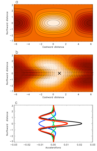
Figure 2.— An example linear, analytic solution for parameters relevant to hot, tidally locked exoplanets. (a) Spatial structure of radiative-equilibrium height field, $h_{\rm eq}$ (orangescale and contours). (b) Height field (orangescale) and horizontal wind velocities (arrows) for the linear, analytic solution forced by relaxation to the $h_{\rm eq}$ profile shown in panel (a) and with nondimensional zonal wavenumber $k=0.5$ and nondimensional radiative and drag times $\tau_{\rm rad}=\tau_{\rm drag}=5$. For a hot Jupiter or hot super Earth, these correspond to dimensional zonal wavelengths of a planetary circumference and dimensional radiative and drag time constants of $\sim$$10^{5}\rm\,sec$ (see Appendix A). In (a) and (b), the horizontal and vertical axes are dimensionless eastward and northward distance, respectively; one unit of distance corresponds to a dimensional distance of one Rossby deformation radius, $(\sqrt{gH}/\beta)^{1/2}$. The $\times$ marks the longitude along the equator where $h$ reaches a maximum and the eddy zonal wind changes sign. (c) Zonal (east-west) accelerations of the zonal-mean flow implied by the linear solution. The black and dark blue curves give the accelerations due to horizontal and vertical eddy transport (terms II and III, respectively, in Eq. 22). The light-green and cyan curves show friction (term IV) and the effect of the mean-meridional circulation (term I), respectively. The red curve shows the sum of all terms. The numerical values adopt a forcing amplitude $\Delta h_{\rm eq}/H=1$. For this value, the nondimensional peak winds approach 0.5, corresponding to speeds of $\sim$$1\rm\,km\sec^{-1}$ on a hot Jupiter.

The solutions exhibit several important features. Although the radiative-equilibrium height field is symmetric in longitude about the substellar point (Fig. 2a), the actual height field deviates significantly from radiative equilibrium and exhibits considerable dynamical structure (Fig. 2b). Two fundamental types of behavior are present. First, at mid-to-high latitudes ($|y|\sim 1$–3 in the figure), the flow exhibits vortical behavior. The dayside contains an anticyclone in each hemisphere, manifesting as a pressure high (i.e., local maximum of the height) around which winds flow clockwise in the northern hemisphere and counterclockwise in the southern hemisphere; the nightside contains a cyclone in each hemisphere, manifesting as a pressure low around which winds flow counterclockwise in the northern hemisphere and clockwise in the southern hemisphere. Second, at low latitudes ($|y|\lesssim 1$), the flows are nearly east-west; they diverge from a point east of the substellar longitude (marked with a cross in Fig. 2b) and converge toward a point east of the antistellar longitude.

As discussed by Gill (1980), these features can be interpreted in terms of forced, damped, steady equatorial wave modes. The mid-to-high latitude feature described above is dynamically analogous to that of an $n=1$ equatorially trapped Rossby wave, which exhibits cyclones and anticyclones—alternating in longitude—that peak off the equator (see Matsuno, 1966, Fig. 4c for an example of the flowfield in this mode). The low-latitude feature discussed above is dynamically analogous to a superposition of the $n=1$ Rossby wave and the equatorial Kelvin wave, which is a fundamental equatorially trapped wave mode with strong zonal winds but very weak meridional winds and whose amplitude is symmetric about, and peaks at, the equator (see, e.g., Holton (2004) or Andrews et al. (1987)). Both of these wave modes exhibit winds that are primarily east-west at the equator; in the example shown in Fig. 2, the Kelvin component dominates over the $n=1$ Rossby component at the equator.

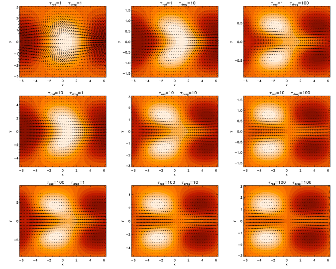
Figure 3.— Analytic solutions of linearized shallow-water equations (Eqs. 16–18), as presented in Appendix B, for dimensionless zonal wavenumber $k=0.5$ and dimensionless radiative and drag time constants of 1, 10, and 100, corresponding roughly to dimensional time constants of 6 hours, 3 Earth days, and one month for parameters appropriate to hot Jupiters (see Appendix A). All of these cases are forced by Newtonian relaxation of the height field toward a distribution analogous to that in Fig. 2a.

Equations (16)–(18) indicate that this is a problem governed by two parameters: the radiative time constant and the drag time constant. We now examine how the behavior depends on their values. Figure 3 shows linear solutions, as presented in Appendix B, for dimensionless radiative time constants of 1, 10, and 100 (top, middle, and bottom rows, respectively) and drag time constants of 1, 10 and 100 (left, middle, and right columns, respectively). For parameters appropriate to hot Jupiters (rotation period of 3 Earth days and $gH\approx 4\times 10^{6}\rm\,m^{2}\sec^{-2}$), these dimensionless values correspond to dimensional time constants of $\sim$$3\times 10^{4}$, $3\times 10^{5}$, and $3\times 10^{6}\rm\,sec$, respectively (see Appendix A). When the radiative and drag time constants are short (upper left corner of Fig. 3), the maximum and minimum thermal (height) perturbations lie on the equator and are close to the substellar and antistellar points; in this limit, the height field is close to radiative equilibrium (compare top left of Fig. 3 with Fig. 2a), and distinct Rossby-wave gyres do not appear. When the radiative and drag time constants have intermediate values (middle of Fig. 3), cyclones and anticyclones become visible and—as in Fig. 2b—exhibit height extrema that are phase shifted westward of the extrema in radiative equilibrium. Similarly, the height extrema along the equator become phase shifted eastward relative to radiative equilibrium; thickness variations along the equator become modest relative to those in midlatitudes. When the radiative and drag time constants are long (lower right corner of Fig. 3), the height field becomes dominated by the off-equatorial anticyclones and cyclones, with minimal variation of height at the equator. In the limits $\tau_{\rm rad}\to\infty$ and $\tau_{\rm drag}\to\infty$, the solution becomes flat at the equator and is symmetric in longitude about the $x=0$ axis (a point demonstrated explicitly in Appendix C); Fig. 3 shows that this limit is almost reached even for $\tau_{\rm rad}$ and $\tau_{\rm drag}$ of 100.

Much of the behavior in Fig. 3 can be understood in terms of the zonal propagation of equatorially trapped Rossby and Kelvin modes. Kelvin waves exhibit eastward group propagation while long-wavelength, equatorially trapped Rossby waves exhibit westward group propagation. When $\tau_{\rm rad}$ and $\tau_{\rm drag}$ are very short (upper left corner of Fig. 3), the damping is so strong that the waves are unable to propagate zonally. As a result, the height is close to the radiative equilibrium height field. When the two time constants have intermediate values, the propagation produces an eastward phase shift of the height field at the equator (the Kelvin component) and a westward phase shift of the height field in the off-equatorial cyclones and anticyclones (the Rossby component)—exactly as seen in Fig. 2b and the middle of Fig. 3. As the two time constants become very long, the westward phase offset of the off-equatorial cyclones and anticyclones achieves maximal values of $90^{\circ}$. At the equator, however, the height variations go to zero; this is explained by the fact that Coriolis forces are zero at the equator, so the linearized force balance is between pressure-gradient forces and drag. Weak drag requires weak pressure-gradient forces and hence a flat layer at the equator.

Now, the key point of our paper is that these linear solutions have major implications for the development of equatorial superrotation on tidally locked exoplanets. As can be seen in Figs. 2b and 3, the wind vectors exhibit an overall tilt from northwest-to-southeast in the northern hemisphere and southwest-to-northeast in the southern hemisphere. This pattern, which resembles a chevron centered at the equator and pointing east, is particularly strong when the radiative and drag time constants are short, but occurs in all the cases shown. This structure implies that, on average, equatorward moving air has faster-than-average eastward wind speed while poleward moving air has slower-than-average eastward wind speed, so that $\overline{u^{\prime}v^{\prime}}<0$ in the northern hemisphere and $\overline{u^{\prime}v^{\prime}}>0$ in the southern hemisphere. As shown schematically in Fig. 1, this is exactly the type of pattern that causes a flux of eastward eddy momentum to the equator and can induce equatorial superrotation. Since momentum is being removed from the mid-latitudes, one would expect westward zonal-mean flow to develop there.

The physical mechanism responsible for producing these phase tilts are twofold. First, the differential wave propagation discussed above: this propagation causes an eastward phase shift of the height field in the Kelvin waves and a westward shift of the height field in the Rossby waves relative to the radiative-equilibrium height field. Because the Rossby wave lies on the poleward flanks of the Kelvin wave, the result is a chevron pattern where the height contours tilt northwest-southeast in the northern hemisphere and southwest-northeast in the southern hemisphere. To the extent that velocity vectors approximately parallel the geopotential contours (as they tend to do away from the equator when drag is weak or moderate), this will generate tilts in the velocities such that $\overline{u^{\prime}v^{\prime}}<0$ in the northern hemisphere and $\overline{u^{\prime}v^{\prime}}>0$ in the southern hemisphere.

The second mechanism for generating the velocity tilts needed for equatorial superrotation is simply the three-way force balance between Coriolis, drag, and pressure-gradient forces. Because drag acts opposite to the velocity, and Coriolis forces are perpendicular to the velocity, this three-way force balance requires the velocities to be rotated clockwise of $-\nabla\eta$ in the northern hemisphere and counterclockwise of $-\nabla\eta$ in the southern hemisphere. Given the expected day-night gradients in $\eta$, this balance implies that the velocities will tend to tilt northwest-southeast in the northern hemisphere and southwest-northeast in the northern hemisphere. We demonstrate this fact explicitly with an analytic solution in the limit of $\tau_{\rm rad}\to 0$ in Appendix D; even when the height field is nearly in radiative equilibrium and hence exhibits no overall phase tilts, the velocities themselves develop tilts such that $\overline{u^{\prime}v^{\prime}}<0$ in the northern hemisphere and $\overline{u^{\prime}v^{\prime}}>0$ in the southern hemisphere (see Fig. 15). The calculation in the limit $\tau_{\rm rad}\to 0$ is particularly interesting because, in this limit, there is no zonal propagation of the Kelvin and Rossby waves: the radiative damping is infinitely strong and the zonal phase shift of the height field (relative to radiative equilibrium) is zero. This is the dominant mechanism for the velocity tilts in the top-left panel of Fig. 3.

To demonstrate explicitly how superrotation would emerge from these standing-wave patterns, we analyze the zonal accelerations associated with these linear solutions. Decomposing variables into their zonal means (denoted by overbars) and deviations therefrom (denoted with primes) and zonally averaging the zonal-momentum equation (Eq. 9) leads to (e.g., Thuburn & Lagneau, 1999)

$${\partial\overline{u}\over\partial t}=\underbrace{\overline{v}^{*}\left[f-{\partial\overline{u}\over\partial y}\right]}_{I}\underbrace{-{1\over\overline{h}}{\partial\over\partial y}[\overline{(hv)^{\prime}u^{\prime}}]}_{II}$$

$$+\underbrace{\left[{1\over\overline{h}}\overline{u^{\prime}Q^{\prime}}+\overline{R_{u}}^{*}\right]}_{III}\underbrace{-{\overline{u}^{*}\over\tau_{\rm drag}}}_{IV}-{1\over\overline{h}}{\partial(\overline{h^{\prime}u^{\prime}})\over\partial t}$$ (22)

where $a$ is the planetary radius and $\overline{A}^{*}\equiv\overline{hA}/\overline{h}$ denotes the thickness-weighted zonal average of any quantity $A$. Eq. (22) is the shallow-water version of the Transformed Eulerian Mean (TEM) momentum equation, analogous to that in the isentropic-coordinate form of the primitive equations (see Andrews et al., 1987, Section 3.9). On the right-hand side, terms I, II, and III represent accelerations due to (i) momentum advection by the mean-meridional circulation, (ii) the convergence of the meridional flux of zonal eddy momentum, and (iii) correlations between the regions of eddy zonal flow and eddy mass source (essentially vertical eddy-momentum transport). Within this term, the quantity $R_{u}$ is the zonal component of ${\bf R}$ (equal to $-Qu/h$ when $Q>0$ and 0 when $Q<0$). Term IV is frictional drag. The final term represents the time rate of change of the eddy momentum. In the linear limit, all the terms on the right side of Eq. (22) have vanishingly small amplitude and, in this case, the solutions in Figs. 2–3 represent true steady states. At any finite amplitude, however, terms I–IV are nonzero and would cause generation of a zonal-mean zonal flow.

Figure 2c depicts these terms for the example solution presented in Fig. 2b. As expected, horizontal convergence of eddy momentum, term II, causes a strong eastward acceleration at the equator and westward acceleration in the midlatitudes (black curve). On the other hand, the acceleration associated with vertical eddy-momentum transport, term III, is strong and westward at the equator (blue), implying downward transport of eddy momentum at the equator. The remaining terms—the mean-meridional circulation (term I, cyan) and mass-weighted friction (term IV, light green)—are small at the equator. The two eddy terms partially cancel at the equator, but the acceleration due to horizontal eddy momentum convergences exceeds that due to vertical eddy momentum convergences, leading to a net eastward acceleration at the equator and westward acceleration in midlatitudes (red curve).

Remarkably, despite the wide range of morphologies that occur when $\tau_{\rm rad}$ and $\tau_{\rm drag}$ are varied (Fig. 3), all the solutions exhibit an equatorward flux of eddy momentum and a net eastward acceleration at the equator. This is shown in Fig. 4, which presents the two eddy acceleration terms from Eq. (22) for each of the cases shown in Fig. 3. These solutions therefore suggest that superrotation at the equator and westward mean flow in the midlatitudes should occur at essentially any value of the control parameters.

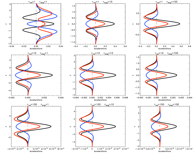
Figure 4.— Accelerations of the zonal-mean zonal flow for the same solutions as in Fig. 3. Black curve is acceleration due to horizontal eddy-momentum convergence (term II in Eq. 22), and blue curve is acceleration due to vertical eddy-momentum transport (term III). Red curve is sum of terms I, II, III, and IV. Numerical values plotted here assume that $\hat{S}_{0}/\tau_{\rm rad}$ (which is essentially equivalent to $\Delta h_{\rm eq}/H$) equals one.

The patterns of spatial velocity and mass source/sink illuminate the physical origin of the westward equatorial acceleration caused by the vertical eddy exchange. The solutions show that the longitudes of zero zonal wind at the equator lie east of the mass-source extrema (Fig. 2b), a feature also clearly visible in the steady, linear calculations of Matsuno (1966, Fig. 9) and Gill (1980, Fig. 1). Because of this shift, equatorial mass sources (sinks) occur predominantly in regions of westward (eastward) eddy zonal flow. On average, therefore, the mass sink regions transport air with eastward column-integrated eddy momentum out of the layer. The mass source regions transport air with no relative zonal momentum from the quiescent abyssal layer into the upper layer; this process conserves the local, column-integrated relative momentum ${\bf v}h$ of the upper layer. Thus, when zonally averaged, vertical exchange at the equator removes momentum from the layer, leading to $(\overline{u^{\prime}Q^{\prime}}+\overline{R_{u}}^{*})<0$ and contributing a westward acceleration (blue curve in Fig. 2c).

The above argument, however, does not determine which of the two eddy terms (II and III in Eq. 22) dominates. To determine which is larger—and hence whether the net equatorial eddy acceleration is eastward or westward—we write the zonally averaged zonal momentum equation in the form

$${\partial\overline{u}\over\partial t}=\overline{v^{\prime}\zeta^{\prime}}+\overline{v}(f+\overline{\zeta})-{\overline{u}\over\tau_{\rm drag}}+\overline{R_{u}}.$$ (23)

where $\zeta$ is the relative vorticity. For the case where the forcing is symmetric about the equator, the solutions are symmetric about the equator in $u$ and $h$ but antisymmetric about the equator in $v$ and $\zeta$. As a result, the meridional velocity and relative vorticity are zero at the equator, so the terms $\overline{v}(f+\zeta)$ and $\overline{v^{\prime}\zeta^{\prime}}$ vanish there. Therefore,

$${\partial\overline{u}\over\partial t}=-{\overline{u}\over\tau_{\rm drag}}+\overline{R_{u}}\qquad\qquad{\rm at}\;y=0.$$ (24)

Essentially, at the equator, $\overline{R_{u}}$ is the mismatch between the accelerations caused by horizontal and vertical eddy-momentum fluxes. The analytic solutions, which assume $\overline{u}=0$, show that $u$ is predominantly westward in regions where $Q>0$, which therefore implies that $\overline{R_{u}}>0$. From Eq. (24), the net eddy-induced acceleration is therefore eastward. This explains, in a general way, the sign of the net eddy accelerations at the equator in Fig. 4. Of course, once a zonal-mean flow ($\overline{u}\neq 0$) develops, the magnitude of $\overline{R_{u}}$ changes and the friction term becomes important in Eq. (24); eventually these terms balance and allow a steady state to be achieved. We discuss the possible steady states in light of this equation in §3.2.

We have so far emphasized the spatial patterns of the circulation, but it is also interesting to examine the magnitudes of the velocities predicted by our linear solutions. When the day-night difference in the radiative-equilibrium height is comparable to the mean value and the radiative time constant is a few days or less (as expected for the strongly forced conditions on hot Jupiters), the winds shown in Fig. 2b and Fig. 3 reach nondimensional speeds of order unity. For a hot Jupiter, with typical $g=20\rm\,m\sec^{-2}$ and $H=200\rm\,km$, this corresponds to dimensional speeds of $\sim$$2\rm\,km\,sec^{-1}$. To within a factor of a few, this is similar to the speeds obtained in fully nonlinear three-dimensional atmospheric circulation models of hot Jupiters (Showman & Guillot, 2002; Cooper & Showman, 2005; Showman et al., 2008, 2009; Dobbs-Dixon & Lin, 2008; Dobbs-Dixon et al., 2010; Menou & Rauscher, 2009; Rauscher & Menou, 2010; Thrastarson & Cho, 2010). For a tidally locked, Earth-like planet in the habitable zone of an M-dwarf, with $g=10\rm\,m\sec^{-2}$, $H=10\rm\,km$, and an Earth-like radiative time constant of $\sim$10 days (corresponding to dimensionless time constants of 10–100), the solutions then yield nondimensional speeds of $\sim 0.02$–0.1. This corresponds to dimensional speeds of up to a few tens of $\rm\,m\sec^{-1}$, similar to speeds obtained in models of tidally locked terrestrial planets (Joshi et al., 1997; Heng & Vogt, 2010; Merlis & Schneider, 2010).

3.2. Nonlinear solutions

Next, we relax the small-amplitude and Cartesian constraints to demonstrate how nonlinearity and full spherical geometry affect the solutions, and we show how the wave-induced accelerations interact with the mean flow to generate an equilibrated state exhibiting equatorial superrotation. To do so, we solve the fully nonlinear forms of Eqs. (9)–(11) in global, spherical geometry, using a radiative-equilibrium thickness given by

$$h_{\rm eq}=H+\Delta h_{\rm eq}\cos\lambda\cos\phi$$ (25)

where $H$ is the mean thickness, $\Delta h_{\rm eq}$ is the day-night contrast in radiative-equilibrium thickness, and the substellar point is at longitude $0^{\circ}$ and latitude $0^{\circ}$. The planet is assumed to be synchronously rotating, so that the pattern of $h_{\rm eq}(\lambda,\phi)$ remains fixed in time. For concreteness, we adopt planetary parameters appropriate to a hot Jupiter, although we expect qualitatively similar solutions to apply to super Earths. For a typical gravity of $20\rm\,m\,sec^{-2}$ and scale height of $200\rm\,km$ appropriate to hot Jupiters, we might expect $gH=4\times 10^{6}\rm\,m^{2}\,sec^{-2}$, and we adopt this value for all our runs. (Note that $g$ and $H$ do not need to be specified independently.) We also take $\Omega=3.2\times 10^{-5}\rm\,sec^{-1}$ and $a=8.2\times 10^{7}\rm\,m$, corresponding to rotation period and planetary radius of 2.3 Earth days and 1.15 Jupiter radii, respectively, similar to the values for HD 189733b.

We reiterate that the equations represent a two layer system with an active layer overlying a quiescent, infinitely deep lower layer. Because of coupling between the layers (specifically, mass exchange in the presence of heating/cooling), the solutions readily reach a steady state for any value of the drag time constant, including the limit where drag is excluded entirely in the upper layer ($\tau_{\rm drag}\to\infty$). This in fact is a simple representation of the situation in many full 3D GCMs of Solar System atmospheres, including Earth, which often have strong frictional drag near the surface, little-to-no friction in the upper layers, and yet easily reach a steady configuration throughout all the model layers. In our case, we find that, when drag is strong, the solutions reach steady states in runtimes $\lesssim 10\tau_{\rm drag}$. In the case where drag is turned off, the time to reach steady state is determined by the magnitude of momentum and energy exchange between the layers (e.g., by the magnitude of the ${\bf R}$ term), and is generally $\lesssim 10\tau_{\rm rad}|H/\Delta h|$, where $|\Delta h|/H$ is a characteristic value of the fractional height variations in the active layer. All solutions shown here are equilibrated and steady.

We solve Eqs. (9)–(11) using the Spectral Transform Shallow Water Model (STSWM) of Hack & Jakob (1992). Rather than integrating the equations for $u$ and $v$, the code solves the momentum equations in a vorticity-divergence form. The initial condition is a flat layer of geopotential $gH$ at rest; the equations are integrated using a spectral truncation of T170, corresponding to a resolution of $0.7^{\circ}$ in longitude and latitude (i.e., a global grid of $512\times 256$ in longitude and latitude). A $\nabla^{6}$ hyperviscosity is applied to each of the dynamical variables to maintain numerical stability. The code adopts the leapfrog timestepping scheme and applies an Asselin filter at each timestep to suppress the computational mode. These methods are standard practice; for further details, the reader is referred to Hack & Jakob (1992).

To facilitate comparison with the analytic theory in §3.1, we first describe the solutions at very low amplitude where the behavior is linear. Figure 5 shows the geopotential (i.e., $gh$) for equal radiative and drag time constants of 0.1, 1, and 10 (Earth) days, respectively. Qualitatively, the numerical solutions in spherical geometry bear a striking resemblance to the analytic solutions on a $\beta$ plane. At time constants of a fraction of day, the geopotential maxima occur on the equator, and for time constants of 0.1 day (a), the geopotential resembles the radiative-equilibrium solution, with wind flowing from the substellar point to the antistellar point. Longer time constants (1 day, panel b) allow zonal energy propagation of the Kelvin and Rossby waves, leading to an eastward phase shift of the geopotential at the equator and a westward phase shift at high latitudes ($\sim$40–$90^{\circ}$). The result is contours of geopotential that develop northwest-southeast tilts in the northern hemisphere and southwest-northeast tilts in the southern hemisphere. When the time constants are long (10 days, panel c) off-equatorial cyclones and anticyclones dominate the geopotential, with only weak geopotential variations along the equator. These vortices are oval in shape, exhibiting no overall phase tilt, though the regions close to the equator do develop phase tilts (westward-poleward to easward-equatorward). The momentum fluxes cause a prograde eddy acceleration (and superrotation) at the equator for all these cases. All of these features are also shared by the analytic solutions (Fig. 3).

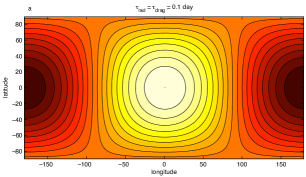
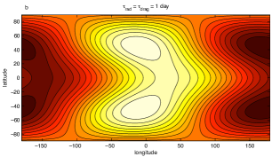
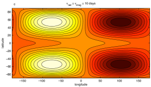
Figure 5.— Geopotential $gh$ (orangescale and contours) for the equilibrated (steady-state) solutions to the shallow-water equations (Eqs. 9–11) in full spherical geometry assuming equal radiative and drag time constants of 0.1, 1, and 10 days in (a), (b), and (c), respectively. White is thick and dark is thin. Although the equations solved are fully nonlinear, the forcing amplitude is small here ($\Delta h_{\rm eq}/H=0.01$) so that the solutions in these panels are essentially linear.

We now explore how the solutions change when the radiative and frictional time scales are different. In the linear limit, the latitudinal width of the region exhibiting prograde phase tilts (i.e., northwest-to-southeast in the northern hemisphere and southwest-to-northeast in the southern hemisphere) contracts toward the equator when the drag time constant greatly exceeds the radiative time constant. This is illustrated in Fig. 6, which shows the equilibrated (steady-state) solutions for $\tau_{\rm rad}=1\rm\,day$ and $\tau_{\rm drag}/\tau_{\rm rad}=1$ (top), 10 (middle), and infinite (bottom). When the time constants are equal, the entire northern (southern) hemisphere exhibits northwest-to-southeast (southwest-to-northeast) phase tilts. When $\tau_{\rm drag}/\tau_{\rm rad}=10$, these phase tilts are confined within $\sim$$20^{\circ}$ latitude of the equator, and for $\tau_{\rm drag}\to\infty$, the width shrinks toward zero. This behavior is explained by the analytic theory in §3.1. As shown in Eq. (20), the parabolic cylinder functions comprising the latitudinal structure exhibit a characteristic latitudinal width of $L(\tau_{\rm rad}/\tau_{\rm drag})^{1/4}$, where $L=(\sqrt{gH}/\beta)^{1/2}$ is the equatorial Rossby deformation radius; these functions thus collapse toward the equator as $\tau_{\rm drag}/\tau_{\rm rad}$ becomes infinite. Poleward of this region, the solutions exhibit phase tilts of the opposite direction (northeast-to-southwest in the northern hemisphere and southeast-to-northwest in the southern hemisphere). Appendix C gives the explanation for this reversal in phase tilts; the low-amplitude, full spherical numerical solutions at $\tau_{\rm drag}/\tau_{\rm rad}\gg 1$ strongly resemble analytic solutions in the absence of drag, presented in Appendix C (compare Figs. 6c and 14).

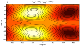
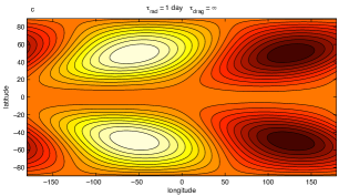
Figure 6.— Geopotential $gh$ (orangescale and contours) for the equilibrated (steady-state) solutions to the shallow-water equations (Eqs. 9–11) in full spherical geometry illustrating the effect of varying $\tau_{\rm drag}$ in the linear limit. All of the cases depicted have $\tau_{\rm rad}=1\,\rm day$. The drag time constant is 1 day, 10 days, and infinite in the top, middle, and bottom panels, respectively. White is thick and dark is thin. As in Fig. 5, $\Delta h_{\rm eq}/H=0.01$ here.

Nonlinearity alters the solutions in several important ways, which we illustrate in Fig. 7, showing a sequence of solutions for $\tau_{\rm rad}=0.1\rm\,day$, $\tau_{\rm drag}=10\rm\,days$ and, from top to bottom, amplitudes $\Delta h_{\rm eq}/H$ of 0.01, 0.1, and 0.5, respectively. This choice of time constants is representative of the regime of strong radiative forcing and weak drag that may be appropriate to typical hot Jupiters. Increasing the forcing amplitude (i.e., increasing $\Delta h_{\rm eq}/H$ while holding $\tau_{\rm rad}$ and $\tau_{\rm drag}$ constant) of course leads to increased wind speeds and day-night geopotential variations; for the parameters in Fig. 7, the zonal-mean zonal wind speed at the equator ranges from $\sim$$10\rm\,m\,sec^{-1}$ at the lowest amplitude to almost $1000\rm\,m\,sec^{-1}$ for the highest amplitude shown. Moreover, beyond a critical value of $\Delta h_{\rm eq}/H$ (depending on the values of $\tau_{\rm rad}$ and $\tau_{\rm drag}$), the solutions begin to deviate qualitatively from the linear solutions.

First, nonlinearity allows greater geopotential variations to occur along the equator, such that at extreme forcing amplitude the geopotential extrema can in some cases occur along the equator when they otherwise would not. In the linear limit, the zonal force balance at the equator in the steady state is between the pressure-gradient force and drag (cf Eq. 13); therefore, when drag is weak, the pressure-gradient force must likewise be small, implying that minimal variations of geopotential occur along the equator. This restriction does not apply at higher latitudes (where the Coriolis force can balance the pressure-gradient force), so for very weak drag the thickness extrema generally occur off the equator (as can be seen in the lower right portion of Fig. 3; Fig. 5b and c; Fig. 6, and Fig. 7a). At large forcing amplitude, however, the momentum advection term ${\bf v}\cdot{\nabla h}$ and the ${\bf R}$ terms become important and can balance the pressure-gradient force, allowing significant zonal pressure gradients—and hence significant variations in thickness—to occur along the equator. For the parameters in Fig. 7, the thickness variations peak at the equator when the forcing amplitude is sufficiently large (bottom panel).

Second, at high amplitude, the phase tilts of wind and geopotential tend to be from northwest-to-southeast (southwest-to-northeast) throughout much of the northern (southern) hemisphere—as in Fig. 7b and 7c— even when the phase tilts are in the opposite direction at low amplitude (as in Fig. 7a). This effect can be directly attributed to the term ${\bf R}$ in the momentum equations. As shown in Eq. (12), ${\bf R}$ plays a role analogous to drag. When true drag is weak or absent, the effective drag time constant (one over the quantity in square brackets in Eq. 12) has a characteristic magnitude $\tau_{\rm rad}h/(h_{\rm eq}-h)$. At large forcing amplitude, $h/(h_{\rm eq}-h)\sim 1$, and in that case the effective drag time constant is comparable to $\tau_{\rm rad}$. The linear solutions show that prograde phase tilts dominate over much of the globe when the radiative and drag time constants are comparable, but when the drag time constant greatly exceeds the radiative time constant, the phase tilts are in the opposite direction (see Fig. 6). In Fig. 7, $\tau_{\rm drag}/\tau_{\rm rad}=100$, but the ratio of the effective drag time constant to the radiative time constant decreases from top to bottom and reaches $\sim$1 in the bottom panel, explaining the transition in the phase tilts from Fig. 7a through 7c. Through the momentum fluxes that accompany these phase tilts, the equatorial jet becomes broader and more dominant with increasing nonlinearity.

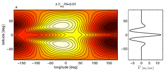
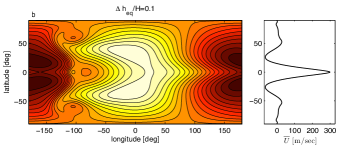
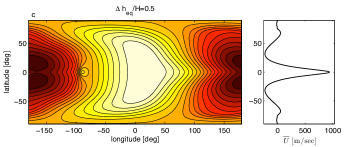
Figure 7.— Geopotential $gh$ (orangescale and contours) for the equilibrated solutions to the shallow-water equations (Eqs. 9–11) in full spherical geometry illustrating the effect of nonlinearity. All of the cases depicted have $\tau_{\rm rad}=0.1\,$ day and $\tau_{\rm drag}=10\,$ days. The forcing amplitude is $\Delta h_{\rm eq}/H=0.01$ 0.1, and 0.5 in (a), (b), and (c), respectively. White is thick and dark is thin. Range of $gh$ values is 3.97–$4.03\times 10^{6}\rm\,m^{2}\sec^{-2}$, 3.6–$4.3\times 10^{6}\rm\,m^{2}\sec^{-2}$, and 2.1–$5.5\times 10^{6}\rm\,m^{2}\sec^{-2}$ from top to bottom, respectively. The solution in (a) is steady; those in (b) and (c) exhibit small-scale eddy generation and time variability (most evident in panel b), although the global properties (total kinetic energy, potential energy, and equatorial jet speed) are essentially constant in time.

The momentum balance in the equatorial jet can achieve steady state in two ways. In steady state, Eq. (24) becomes

$${\overline{u}\over\tau_{\rm drag}}=\overline{R_{u}}\qquad\qquad({\rm at\;the\;equator}).$$ (26)

As described previously, when the zonal-mean zonal winds are weak, the zonal wind $u$ is predominantly westward in regions where $Q>0$, so that $\overline{R_{u}}>0$ (§3.1 and Fig. 4). This implies an eastward eddy acceleration of the zonal-mean zonal winds at the equator, which induces equatorial superrotation. In the first type of steady state, corresponding to a regime of strong friction (short drag time constant), this superrotation implies a strong westward acceleration due to friction ($-\overline{u}/\tau_{\rm drag}$). Steady state occurs when the zonal-mean equatorial jet becomes strong enough for the friction to balance the eastward eddy-induced acceleration at the equator. We call this the “high Prandtl number” regime. In the second type of steady state, which we call the “low Prandtl number” regime, the friction is sufficiently weak that the term $-\overline{u}/\tau_{\rm drag}$ is unimportant in the momentum balance. Because of the eastward eddy acceleration, the zonal-mean zonal winds can build to high speed. Once they do, they change the nature of $\overline{R_{u}}$—the larger $\overline{u}$ becomes, the smaller the extent to which $u<0$ in the region $Q>0$, as necessary for $\overline{R_{u}}>0$. Eventually, for sufficiently large $\overline{u}$, the quantity $\overline{R_{u}}$ goes to zero at the equator. The equatorial jet thus achieves steady state.

Figure 8 shows examples of each of these regimes illustrating how the momentum balance occurs. The left column presents an example with strong drag ($\tau_{\rm rad}=\tau_{\rm drag}=1\rm\,day$) and the right column presents an example with weak drag ($\tau_{\rm rad}=0.1\rm\,day$ and $\tau_{\rm drag}=\infty$); both are equilibrated and steady. These are high-amplitude cases, so the thickness (top row, a and e) exhibits large fractional variations, and the phase tilts exhibit an overall trend of northwest-to-southeast (southwest-to-northeast) in the northern (southern) hemisphere, as explained in previous discussion (cf Fig. 7). These tilts indicate transport of eddy momentum from midlatitudes to the equator; as a result, the zonal-mean zonal winds are eastward at the equator and westward in the midlatitudes (b and f). Interestingly, however, the relative strengths of the equatorial and midlatitude jets differ and reflect the range of possible variation. Panels (c) and (g) show the terms in the zonal-mean momentum equation, just the spherical equivalent of Eq. (22):

$${\partial\overline{u}\over\partial t}=\underbrace{\overline{v}^{*}\left[f-{1\over a\cos\phi}{\partial(\overline{u}\cos\phi)\over\partial\phi}\right]}_{I}$$

$$\underbrace{-{1\over\overline{h}a\cos^{2}\phi}{\partial\over\partial\phi}[\overline{(hv)^{\prime}u^{\prime}}\cos^{2}\phi]}_{II}$$

$$+\underbrace{\left[{1\over\overline{h}}\overline{u^{\prime}Q^{\prime}}+\overline{R_{u}}^{*}\right]}_{III}\underbrace{-{\overline{u}^{*}\over\tau_{\rm drag}}}_{IV}-{1\over\overline{h}}{\partial(\overline{h^{\prime}u^{\prime}})\over\partial t}.$$ (27)

As expected, horizontal convergence of eddy momentum, term II, causes a strong eastward acceleration at the equator and westward acceleration in midlatitudes (black curves). The vertical eddy-momentum transport, term III (dark blue curves), causes a westward acceleration at the equator that counteracts the eastward acceleration due to horizontal eddy-momentum convergence. In the case of strong drag (Fig. 8c), the cancellation is imperfect, leading to a net eddy-induced acceleration that is eastward at the equator—as predicted by the linear, analytic theory in §3.1 (compare to Fig. 2c). A superrotating equatorial jet therefore emerges and only reaches steady state when the jet becomes sufficiently strong that the zonal-mean drag on the jet, $-\overline{u}^{*}/\tau_{\rm drag}$, balances the eastward acceleration at the equator (Fig. 8c). On the other hand, when drag is absent, the superrotation induced by the eddy fluxes becomes quite strong (Fig. 8f). This mean flow alters the eddy fluxes, causing them to self-adjust to an equilibrium where the accelerations at the equator due to horizontal and vertical momentum fluxes cancel, leading to no net eddy-induced acceleration at the equator in steady state (Fig. 8g).

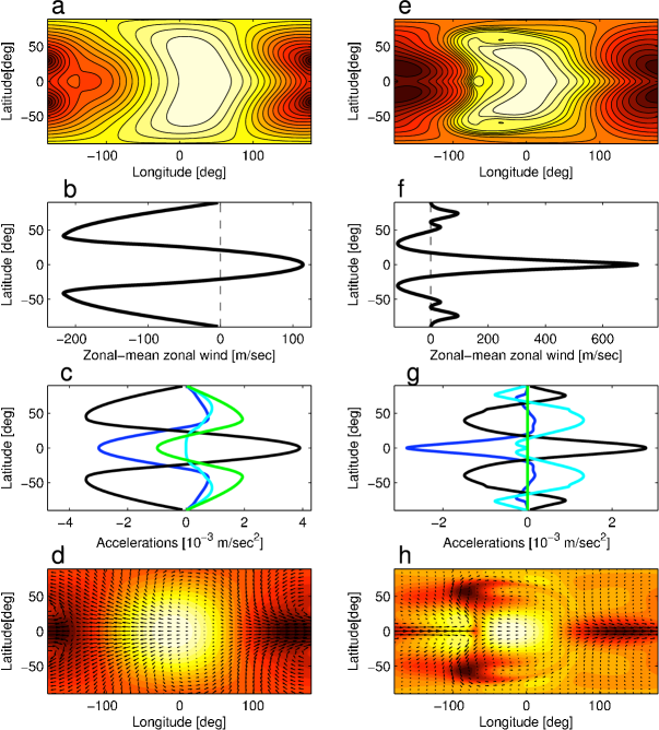
Figure 8.— Fully nonlinear shallow-water solutions with $\tau_{\rm rad}=1\rm\,day$, $\tau_{\rm drag}=1\rm\,day$, and $\Delta h_{\rm eq}/H=1.25$ (left column) and $\tau_{\rm rad}=0.1\rm\,day$, no drag ($\tau_{\rm drag}\to\infty$), and $\Delta h_{\rm eq}/H=0.2$ (right column). (a, e) Geopotential $gh$ (orangescale and contours, with thick and thin regions in white and black, respectively). Scale runs from $1.1$–$5.4\times 10^{6}\rm\,m^{2}\,sec^{-2}$ in top panel and $3.3$–$4.6\times 10^{6}\rm\,m^{2}\,sec^{-2}$ in bottom panel. (b, f) Zonal-mean zonal wind $\overline{u}$. (c, g) Accelerations of the zonal-mean zonal wind in the equilibrated state. From Eq. (27), curves are terms I (cyan), II (black), III (dark blue), IV (light green). (d, h) Mass source $gQ$ at the equator (orangescale, white being positive and dark being negative values) and winds (arrows). Mass source scale runs from $-41.3$ to $45.1\rm\,m^{2}\sec^{-3}$ (left) and $-38.1$ to $33.2\rm\,m^{2}\sec^{-3}$ (right).

We find that equatorial superrotation occurs at all forcing amplitudes, even arbitrarily small amplitudes where the solutions behave linearly. This is illustrated in Fig. 9, which shows the equilibrated equatorial zonal-mean zonal wind versus forcing amplitude for solutions with a range of $\tau_{\rm rad}$ and $\tau_{\rm drag}$ combinations. We therefore conclude that the mechanism for generating equatorial superrotation described here has no inherent threshold. Nevertheless, other processes—not included in the shallow-water model—can in some cases overwhelm the desire of the day-night forcing to trigger superrotation, particularly when the day-night forcing is weak. This occurs for example in the cases examined by Suarez & Duffy (1992) and Saravanan (1993), where superrotation only developed for forcing amplitudes exceeding a threshold value. In their case, the tropical wave forcing only triggers superrotation when it attains sufficiently great amplitudes to overcome the westward torques provided by midlatitude eddies propagating into the tropics. These issues are discussed further in §5.

In all the cases shown in Fig. 9 where $\tau_{\rm drag}$ is finite, the zonal-mean speed of equatorial superrotation scales with the square of the forcing amplitude when the forcing amplitude is sufficiently small. This in fact is the expected low-amplitude behavior in the high-Prandtl-number regime described above: at low amplitude, the solutions become linear, such that the velocities, height perturbations, and mass source/sink scale with the forcing amplitude. Because $\overline{R_{u}}$ scales as the product of the mass source/sink and the velocities at low amplitude, it is therefore quadratic in the forcing amplitude. In the frictional regime, Eq. (26) implies that $\overline{u}$ at the equator is simply $\tau_{\rm rad}\overline{R_{u}}$, and therefore $\overline{u}$ itself is quadratic in the forcing amplitude. This behavior breaks down when the solutions become sufficiently high amplitude, as can be seen in Fig. 9. The low-Prandtl-number regime is more complex and can lead to a variety of scaling behaviors depending on the parameters.

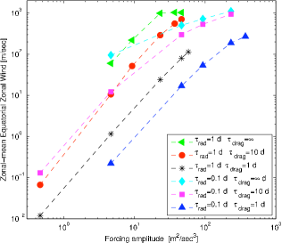
Figure 9.— Equilibrated (steady-state) equatorial jet speed from the nonlinear shallow-water solutions for a variety of forcing amplitudes, radiative time constants, and drag time constants. The jet is eastward (i.e., superrotating) in all cases. In most cases, the zonal-mean jet speed scales as forcing amplitude squared at low amplitude but exhibits a flatter dependence at high amplitude. Here, forcing amplitude is defined as $g\Delta h_{\rm eq}/\tau_{\rm rad}$.

The flow in the shallow-water models differ from that in 3D models in one major respect. In many three-dimensional models of hot Jupiters, eastward equatorial flow occurs not only in the zonal mean but at all longitudes, at least over some range of pressures. In contrast, although the shallow-water models described here all exhibit eastward zonal-mean flow at the equator, the zonal wind at the equator is always westward over some range of longitudes. This can be seen as follows: $\overline{R_{u}}$ is essentially the mismatch in equatorial zonal acceleration between horizontal and vertical eddy-momentum transport and in steady state, when $\overline{u}>0$, will be greater than or equal to zero. From the definition of $R_{u}$, this implies westward equatorial flow at some longitudes. This trait probably arises because the meteorologically active atmosphere has here been resolved with only one layer overlying a deep interior; in future work, it would be interesting to explore models that represent the flow with two or more layers overlying a quiescent interior to see whether they can develop equatorial flow that is eastward at all longitudes.

4. Three-dimensional model of equatorial superrotation

Here, we show how the basic mechanism for generating equatorial superrotation identified in §3 occurs also in three dimensions under realistic conditions. To do so, we analyze the three-dimensional model of HD 189733b presented in Showman et al. (2009). Showman et al. (2009) coupled the dynamical core of the MITgcm (Adcroft et al., 2004), which solves the primitive equations of meteorology in global, spherical geometry, using pressure as a vertical coordinate, to the state-of-the-art, non-gray radiative transfer scheme of Marley & McKay (1999), which solves the multi-stream radiative transfer equations using the correlated-k method to treat the wavelength dependence of the opacities. This coupled model, dubbed the Substellar and Planetary Atmospheric Circulation and Radiation (SPARC) model, is to date the only GCM to include realistic radiative transfer for hot Jupiters. Gaseous opacities were calculated assuming local chemical equilibrium for a specified atmospheric metallicity, assuming rainout of any condensates (i.e. ignoring cloud opacity). Showman et al. (2009) presented synchronously rotating models of HD 189733b with one, five, and ten times solar metallicity and of HD 209458b with solar metallicity, along with several models with non-synchronous rotation. Their HD 189733b models in particular compare favorably with a variety of observational constraints (Showman et al., 2009; Agol et al., 2010), and here we focus on their solar-metallicity, synchronously rotating HD 189733b case. This model adopts planetary radius and gravity of $8.24\times 10^{7}\rm\,m$ and $9.36\rm\,m\,sec^{-2}$. The rotation rate is $3.3\times 10^{-5}\rm\,sec$, corresponding to a rotation period of 2.2 Earth days.

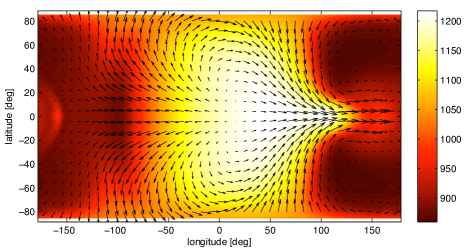
Figure 10.— Temperature (colorscale, in K) and winds (arrows) during the spin-up phase of the three-dimensional, solar-metallicity model of HD 189733b from Showman et al. (2009). This shows the state at the 30-mbar pressure level—near the mean infrared photosphere—at a time of one Earth day, after the day-night forcing has generated a global wave response but before strong zonal-mean jets have developed. Substellar point is at $0^{\circ}$ latitude, $0^{\circ}$ longitude. Note the development of a “Matsuno-Gill”-type pattern, which leads to an equatorward flux of eddy momentum that pumps the equatorial jet.

Figure 10 shows the velocity and temperature structure at the 30-mbar level during the spin-up phase of this model—after the forcing has had sufficient time to trigger a global wave response but before the equatorial jet has spun up to high speed. The velocity pattern in the three-dimensional model (Fig. 10) strongly resembles the standing Kelvin and Rossby-wave pattern described in §3. The flow clearly exhibits the east-west divergence along the equator, emanating from a point near the substellar longitude, identified in §3 as the standing Kelvin-wave response. The longitude of peak divergence (i.e., the longitude at the equator where the zonal velocity changes sign) lies east of the substellar longitude, as expected from the analytic theory and nonlinear shallow-water runs in §3. Moreover, the flow exhibits the broad gyres in each hemisphere, anticyclonic on the dayside and cyclonic on the nightside, identified in §3 as the standing Rossby-wave response. As predicted analytically, the velocities in these gyres exhibit a northwest-to-southeast (southwest-to-northeast) phase tilt in the northern (southern) hemisphere. These phase tilts imply that $\overline{u^{\prime}v^{\prime}}$ is negative in the northern hemisphere and positive in the southern hemisphere. Eddy momentum therefore fluxes from the midlatitudes to the equator, and it is this flux that produces the superrotating equatorial jet (see Fig. 1). The overall qualitative resemblance to the analytic calculation in Fig. 2 is striking.

As in the shallow-water solutions, the three-dimensional models exhibit a net downward eddy momentum flux at the equator throughout the upper atmosphere where the radiative heating/cooling is strong. This momentum flux results from the fact that, at the equator, (i) the Matsuno-Gill-type standing-wave patterns lead to net zonal eddy velocities that are predominantly westward on the dayside and eastward on the nightside (see Fig. 10), and (ii) net radiative heating occurs on much of the dayside, leading to net upward velocities, whereas net radiative cooling occurs on the nightside, leading to net downward velocities. Thus, at the equator, upward velocities tend to be correlated with westward eddy velocities and vice versa. This transports eastward momentum downward and causes a westward acceleration at the equator throughout the upper atmosphere, which counteracts the eastward equatorial acceleration caused by latitudinal eddy-momentum transport—just as predicted by the analytic and numerical shallow-water solutions in §3 (see Figs. 2, 4, and 8).

To quantify the accelerations resulting from these momentum fluxes, we consider the Eulerian-mean zonal-momentum equation in pressure coordinates. By expanding the dynamical variables into zonal-mean and deviation (eddy) components, and zonally averaging the zonal-momentum equation, and adopting pressure as the vertical coordinate, we obtain

$${\partial\overline{u}\over\partial t}=\overline{v}\left[f-{1\over a\cos\phi}{\partial(\overline{u}\cos\phi)\over\partial\phi}\right]-\overline{\omega}{\partial\overline{u}\over\partial p}$$

$$-{1\over a\cos^{2}\phi}{\partial(\overline{u^{\prime}v^{\prime}}\cos^{2}\phi)\over\partial\phi}-{\partial(\overline{u^{\prime}\omega^{\prime}})\over\partial p}+\overline{X}$$ (28)

On the righthand side, the terms describe the meridional momentum advection by the zonal-mean circulation, vertical momentum advection by the zonal-mean circulation, the meridional eddy-momentum convergence, the vertical eddy-momentum convergence, and friction (represented generically by $\overline{X}$), respectively. At the equator, the Coriolis term is zero. Because of the approximate symmetry of the flow about the equator, $\overline{v}$ and the meridional gradient of $\overline{u}$ are small there, so the mean-meridional advection term is small at the equator. The mean vertical-advection term also tends to be weak for the flow considered here, and the net zonal acceleration at the equator is then determined primarily by a competition between the horizontal and vertical eddy-momentum convergence terms (the analogs of terms II and III in Eq. (27) for the shallow-water system).

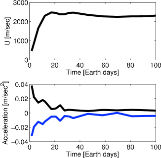
Figure 11.— Time evolution of the upper-atmospheric circulation in the three-dimensional model of HD 189733b by Showman et al. (2009). (Top:) Zonal-mean zonal wind at the equator. (Bottom:) Zonal accelerations due to latitudinal eddy-momentum convergence, $-(a\cos^{2}\phi)^{-1}\partial(\overline{u^{\prime}v^{\prime}}\cos^{2}\phi)/\partial\phi$ (black curve) and vertical eddy-momentum convergence, $-\partial(\overline{u^{\prime}\omega^{\prime}})/\partial p$ (blue curve). All quantities are shown in the upper atmosphere, averaged vertically from 30 mbar to the top of the model.

Figure 11 shows the time evolution of the zonal-mean zonal wind and the two eddy acceleration terms at the equator for the solar-metallicity model of HD 189733b from Showman et al. (2009). These are vertical averages through the top portion of the atmosphere where the radiative heating/cooling is strong. The zonal-mean zonal wind accelerates rapidly from the initial rest state and approaches an equilibrium within $\sim$100 days (top). As expected, the acceleration due to horizontal eddy transport is eastward, while that due to vertical eddy transport is westward (bottom). Moreover, as suggested by the linear and nonlinear shallow-water calculations, the magnitude of the horizontal momentum convergence exceeds that of the vertical momentum convergence during spin-up, so the net acceleration is eastward at early times. A superrotating equatorial jet therefore develops. As the jet speed builds, the two acceleration terms weaken significantly, and the ratio of their magnitudes approaches one. As a result, the net acceleration drops to zero, allowing the jet to equilibrate to a constant speed (top). This model is in the same regime as the shallow-water calculation presented in the right column of Fig. 8.

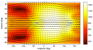
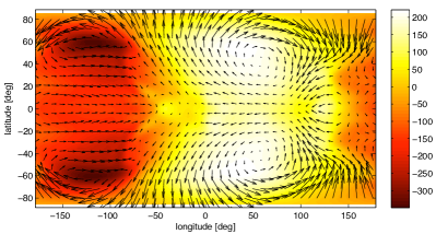
Figure 12.— Top: Temperature (colorscale, in K) and winds (arrows) for the solar-metallicity model of HD 189733b from Showman et al. (2009). Bottom: Eddy temperature $T^{\prime}$ (colorscale, K) and eddy winds $(u^{\prime},v^{\prime})$ (arrows) for the same model. Both are shown at 30 mbar pressure, near the mean infrared photosphere, after the winds at these levels have reached steady state.

The weakening in time of the eddy accelerations seen in Fig. 11 indicates that the mean flow, once it forms, exerts a back-reaction on the eddies that alters their structure. The nature of these changes are illustrated in Fig. 12. The top panel shows the temperatures and winds at 30 mbar pressure after the flow at this altitude has become steady; the superrotating equatorial jet, eastward offset of the hottest region from the substellar point, and other features are evident as detailed in Showman et al. (2009). The bottom panel depicts the eddy temperature and eddy winds for the same pressure and time—that is, $T^{\prime}$ in colorscale and ($u^{\prime}$,$v^{\prime}$) as arrows. Several features are similar to those in Fig. 10: the eddy flow near the equator is approximately zonal and exhibits a Kelvin-wave-like character, with predominantly eastward flow at some longitudes and westward flow at others; the midlatitudes contain broad Rossby-wave gyres in each hemisphere, anticyclonic on the dayside and cyclonic on the nightside. Interestingly, however, the Kelvin-wave structure is shifted eastward, and the midlatitude velocity structure differs significantly, relative to that with weak mean flow (compare Fig. 12b to Figs. 2b and 10). From longitudes of about $-75^{\circ}$ to $+40^{\circ}$, the midlatitude velocity structure induces equatorward momentum flux (i.e., $u^{\prime}v^{\prime}$ negative in the northern hemisphere and positive in the southern hemisphere), but at longitudes $\sim 80$ to $150^{\circ}$ the flux is reversed (i.e., $u^{\prime}v^{\prime}$ positive in the northern hemisphere and negative in the southern hemisphere). Due to this cancellation, the magnitude of the zonally averaged flux $\overline{u^{\prime}v^{\prime}}$ is significantly weaker in the equilibrated state than during the spin-up phase, when the signs of the midlatitude $u^{\prime}v^{\prime}$ add coherently at most longitudes (see Fig. 10).

The latitudinal pattern of zonal-mean eddy accelerations in the upper atmosphere of the 3D model, shown in Fig. 13, exhibit a strong relationship to those from the shallow-water calculations. The comparison is most apt to shallow-water calculations with short radiative time constant ($\tau_{\rm rad}\sim 0.1$–1 day), weak frictional drag ($\tau_{\rm drag}\to\infty$), and large amplitude, as depicted for example in the right column of Fig. 8. In the 3D model (Fig. 13), the acceleration due to horizontal eddy-momentum convergence is eastward at the equator and westward in midlatitudes, in agreement with analytic theory and non-linear shallow-water solutions (compare black curve in Fig. 13 to Figs. 4 and 8g). Near the poles, the situation is more complex. Poleward of $\sim$$50^{\circ}$ latitude, the acceleration in the upper atmosphere of the 3D run is eastward. In the shallow-water solutions, the pattern of eddy accelerations at high latitude depend on $\tau_{\rm rad}$, $\tau_{\rm drag}$, and the forcing amplitude (e.g., compare Figs. 8c and 8g poleward of $\sim$$60^{\circ}$ latitude), but for the shallow-water cases most relevant to the 3D run shown here—such as the right column in Fig. 8—the acceleration due to horizontal eddy convergence becomes eastward at high latitudes (Fig. 8g), like that in the 3D run. In the 3D model, the acceleration due to vertical eddy-momentum convergence (blue curve in Fig. 13) is westward at the equator and eastward in the midlatitudes, again like that arising in the shallow-water solutions, although a significant difference is that the midlatitude eastward acceleration is weak in the shallow-water runs but strong in the three-dimensional run (relative to the magnitude of acceleration at the equator).

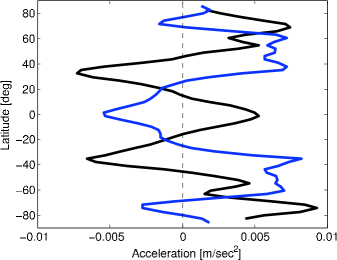
Figure 13.— Zonal-mean zonal accelerations from the solar-metallicity model of HD 189733b from Showman et al. (2009). Black and blue show accelerations due to latitudinal and vertical convergence of eddy momentum, respectively. Both are vertically averaged from 30 mbar to the top of the model at 0.2 mbar and temporally averaged from 11 to 870 days.

Of course, the standing eddy patterns and resulting zonal-wind accelerations in 3D models depend on the strength of radiative heating/cooling and drag, just as they do in the shallow-water models. For example, in the shallow-water solutions, the Kelvin-wave structure and Rossby gyres are spatially distinct when the radiative and/or drag time constants are long and the forcing amplitude is small but not when the time constants are short or the forcing amplitude is large (e.g., compare the upper left versus lower right of Fig. 3, the top versus the bottom of Fig. 5, and the top versus the bottom of Fig. 7). The 3D models shown here lie at an intermediate position along this continuum, with Rossby and Kelvin-wave structures that are visibly distinct, analogous for example to the shallow-water case in Fig. 2b. 3D models with very strong heating rates, however, seem to exhibit eddy patterns lacking distinct Rossby wave gyres, more analogous to the top-left case in Fig. 3 and the top case in Fig. 5. Examples of models in this regime include the topmost part of the atmosphere in the models of Cooper & Showman (2005, 2006), Koskinen et al. (2007), Rauscher & Menou (2010) and the HD 209458b model of Showman et al. (2009). In contrast, cases in the literature with more modest heating rates tend to exhibit distinct standing Rossby and Kelvin-wave structures; examples include Showman & Guillot (2002, Fig. 5), Heng & Vogt (2010, Figs. 1 and 12), the lower portion of some of the models of Koskinen et al. (2007, Fig. 3b), and several of the runs in Thrastarson & Cho (2010), which exhibit a planetary-scale cyclone and anticyclone in each hemisphere.

Despite differences of detail, the overall broad similarities described here between the 3D and shallow-water models argues strongly that the mechanism for equatorial jet maintenance that we have identified occurs in both the shallow-water and 3D models.

5. Discussion

The development of an eastward equatorial jet—that is, equatorial superrotation—is a common feature emerging from three-dimensional models of synchronously rotating hot Jupiters and extrasolar terrestrial planets (Showman & Guillot, 2002; Cooper & Showman, 2005, 2006; Showman et al., 2008, 2009; Dobbs-Dixon & Lin, 2008; Menou & Rauscher, 2009; Rauscher & Menou, 2010; Perna et al., 2010; Heng et al., 2010; Joshi et al., 1997; Merlis & Schneider, 2010; Heng & Vogt, 2010). Showman & Guillot (2002) first pointed out that, when the radiative and advective time constants are similar, this superrotation causes an eastward displacement of the hottest regions from the substellar point—a phenomenon discovered on HD 189733b five years later (Knutson et al., 2007, 2009). Despite its relevance, however, the dynamial mechanisms responsible for generating the equatorial superrotation on tidally locked exoplanets have not been previously identified.

Here, we have shown that the equatorial superrotating jet results from an interaction of the mean flow with standing, planetary-scale Rossby and Kelvin waves generated by the day-night thermal forcing. The strong longitudinal variations in radiative heating—namely intense dayside heating and nightside cooling—trigger the formation of standing, planetary-scale equatorial Rossby and Kelvin waves; this is essentially a linear response when wind speeds are modest, although nonlinearities affect the wave structure at high amplitude. The Kelvin waves straddle the equator while the Rossby waves lie on their poleward flanks. As a result of the differential zonal propagation—Kelvin waves propagating to the east and long-wavelength Rossby waves to the west—as well as the multi-way force balance between pressure-gradient, Coriolis, advective, and drag forces, the velocities develop tilts that resemble an eastward-pointing chevron centered at the equator. These velocity tilts pump eastward momentum from high latitudes to the equator, thereby inducing equatorial superrotation. In steady state, the zonal-mean equatorial jet speed near the photosphere is determined by a balance between this eastward, wave-induced acceleration and westward equatorial acceleration resulting from vertical eddy-momentum transport and/or drag. We demonstrated the mechanism in a hierarchy of dynamical models—including linear, analytic shallow-water models, fully nonlinear shallow-water models, and state-of-the-art three-dimensional GCMs. For conditions relevant to hot Jupiters, such equatorial superrotation occurs over a wide range of radiative heating rates and drag time constants. The consistency of the picture emerging from this sequence of models with widely varying complexity is encouraging and suggests that the mechanism is robust.

The mechanism identified here has several implications:

• It implies that the equatorial jet results from a direct, essentially weakly nonlinear interaction between the thermally forced waves and the mean flow at the planetary scale. Eddy-eddy interactions, including the possibility of inverse or forward energy cascades or other turbulent interactions, may occur but are not essential to the basic mechanism. (This is analogous to the situation suggested by O’Gorman & Schneider (2007) for interaction of baroclinic midlatitude eddies with the mean flow on Earth.)

• The wave-mean-flow interaction produces an equatorial jet whose latitudinal width is comparable to that of the Rossby waves, namely the equatorial Rossby deformation radius modified by radiative and frictional effects. For conditions typical of synchronously rotating hot Jupiters, this length is comparable to a planetary radius, explaining the broad scale of the equatorial jet obtained in most hot Jupiter models.

• When acting in isolation, this mechanism for generating superrotation has no inherent forcing-amplitude threshold; it operates at any forcing amplitude, unlike the behavior reported in some earlier studies in the terrestrial context (Suarez & Duffy, 1992; Saravanan, 1993).

• For parameter combinations appropriate to hot exoplanets, our models yield flows whose hottest regions along the equator lie to the east of the substellar point. This property results from the eastward group propagation of Kelvin waves. The development of a strong mean flow (equatorial superrotation) further enhances the offset by its eastward advection of the temperature pattern. Together, these effects can explain the offsets observed on HD 189733b (Knutson et al., 2007, 2009).

Despite the ubiquity of superrotation in our models, the flow could shift regimes to one with westward zonal-mean equatorial flow if westward equatorial accelerations caused by other processes—not considered here—become important. For example, if baroclinic instabilities occur in midlatitudes, they could cause Rossby wave radiation at midlatitudes, potentially allowing absorption of Rossby waves near the equator. This would contribute a westward wave-induced acceleration near the equator. If this westward acceleration dominates over the eastward equatorial acceleration caused by the day-night heating contrast, then the net wave-induced acceleration at the equator could be westward and equatorial superrotation would not occur. This could occur on hot Jupiters if the planetary rotation rate is sufficiently fast and heating rates are sufficiently low. Note that baroclinic instabilities cannot occur in a one-layer model such as the shallow-water model, helping to explain why no such transitions to westward zonal-mean equatorial flow were seen in the shallow-water models presented here. In some cases, Hadley cells may also force the circulation into a regime of westward equatorial flow, particularly if the planetary obliquity is non-zero; this is the case in Earth’s troposphere. On the other hand, if the planetary rotation is sufficiently slow, additional mechanisms for generating equatorial superrotation become possible, even when the forcing is axisymmetric (Del Genio & Zhou, 1996; Mitchell & Vallis, 2010). Exploring the combinations of orbital semimajor axes, stellar fluxes, planetary rotation rates, and atmospheric compositions under which such regime transitions can occur in 3D models is an important goal for future work, as such transitions could have major implications for visible and infrared light curves.

It is worth mentioning that the presence of a physical surface—and entropy gradients on that surface—promote the existence of baroclinic instabilities in midlatitudes (see for example Vallis, 2006, Chapter 6), so tidally locked terrestrial planets may be more prone than hot Jupiters to experience a regime transition to a flow containing midlatitude eastward jets in addition to, or instead of, a flow dominated by equatorial superrotation.

In the geophysical-fluid-dynamics (GFD) literature, the generation of midlatitude eastward zonal jets is often described theoretically using simple barotropic considerations analogous to those summarized in §2, involving the propagation of waves. While such barotropic considerations seem to work reasonably well for midlatitude jets, the barotropic framework fundamentally fails to explain the emergence of equatorial superrotation in 3D models of synchronously rotating exoplanets, where the flow is often steady and symmetric about the equator. The theory presented here overcomes this obstacle and represents an extension of the barotropic framework to a thermally forced, stratified, ageostrophic flow with finite Rossby deformation radius.

Specifically, the generation of eastward jets is often interpreted in terms of the meridional propagation of Rossby waves away from a source region and their dissipation at other latitudes (e.g., Held, 2000; Vallis, 2006). As described in §2, this interpretation seems to flow naturally from barotropic theory, in which free Rossby waves, even at the equator, can propagate not only in longitude but also in latitude. In contrast, although our work clearly shows how superrotation can emerge on tidally locked planets, meridional wave propagation plays no obvious role in our theory. Unlike barotropic Rossby waves, the baroclinic Rossby waves in our theory are equatorially trapped, confined to an equatorial waveguide: they can propagate in longitude and potentially height but not latitude. Moreover, under conditions appropriate to typical hot Jupiters, these waves exhibit meridional scales typically stretching from the equator to the pole. It is not at all clear that the paradigm of waves propagating from one latitude to another applies in this context. Rather, the velocity tilts that allow the meridional momentum fluxes to generate superrotation appear to be explained by the differential zonal—rather than meridional—propagation of equatorially trapped Kelvin and Rossby waves. Future work may further clarify the issue.

Appendix A A. Non-dimensionalization

The nondimensional solutions to Eqs. (16)–(18) involve three dimensionless parameters — $k$, $\tau_{\rm rad}$, and $\tau_{\rm drag}$. Here we relate these dimensionless parameters to physical properties for exoplanets. For synchronously locked exoplanets, we expect the forcing to correspond to a zonal planetary wavenumber $1$, implying a dimensional wavenumber of $a^{-1}$, where $a$ is the planetary radius. Thus, our dimensionless wavenumber $k$ has the value $a^{-1}(\sqrt{gH}/\beta)^{1/2}$, that is

$$k=\left({\sqrt{gH}\over 2\Omega a}\right)^{1/2}$$ (A1)

If we assume for purposes of illustration that the mean layer thickness $H$ is a scale height, then $gH$ is just $RT$ where $R$ is the specific gas constant and $T$ is the mean temperature of the atmosphere. For a hydrogen atmosphere where $R=3700\rm\,J\rm\,kg^{-1}\rm\,K^{-1}$, this gives

$$k=0.75\left({T\over 1000\rm\,K}\right)^{1/4}\left({P\over 3\,\rm days}\right)^{1/2}\left({R_{\rm J}\over a}\right)^{1/2}$$ (A2)

where $P$ is the rotational period and $R_{J}$ is Jupiter’s radius. For a carbon dioxide atmosphere where $R=189\rm\,J\rm\,kg^{-1}\rm\,K^{-1}$,

$$k=1.2\left({T\over 1000\rm\,K}\right)^{1/4}\left({P\over 3\,\rm days}\right)^{1/2}\left({R_{\oplus}\over a}\right)^{1/2}$$ (A3)

where $R_{\oplus}$ is Earth’s radius. Thus, relevant values of $k$ for a hot Jupiter and a hot Earth are similar, in the range of $\sim$0.5–2. Hotter atmospheres, longer rotation (=orbital) periods, and smaller planetary radii would promote larger values of $k$.

Consider now $\tau_{\rm rad}$ and $\tau_{\rm drag}$. Their nondimensional values are their dimensional values times $(\sqrt{gH}\beta)^{1/2}$. Considering $\tau_{\rm nondim}$ to be either dimenionless time constant ($\tau_{\rm rad}$ or $\tau_{\rm drag}$) and $\tau_{\rm dim}$ to be its dimensional counterpart, we have

$$\tau_{\rm nondim}=\tau_{\rm dim}\left({2\Omega\sqrt{gH}\over a}.\right)^{1/2}$$ (A4)

Again equating $gH$ with $RT$, for a hot Jupiter with a hydrogen atmosphere we obtain

$$\tau_{\rm nondim}=3.6\left({\tau_{\rm dim}\over 10^{5}\sec}\right)\left({R_{J}\over a}\right)^{1/2}\left(T\over{1000{\rm\,K}}\right)^{1/4}\left({3\,{\rm days}\over P}\right)^{1/2}.$$ (A5)

while for a hot Earth with a CO₂ atmosphere

$$\tau_{\rm nondim}=5.7\left({\tau_{\rm dim}\over 10^{5}\sec}\right)\left({R_{\oplus}\over a}\right)^{1/2}\left(T\over{1000{\rm\,K}}\right)^{1/4}\left({3\,{\rm days}\over P}\right)^{1/2}.$$ (A6)

Appendix B B. Analytic solutions for general $\tau_{\rm rad}$ and $\tau_{\rm drag}$

Here we present solutions to the nondimensional, linearized shallow-water equations, (16)–(18), subject to thermal forcing and drag. We follow the solution method outlined by Gill (1980) and Wu et al. (2001). For notational brevity, we define $\alpha\equiv\tau_{\rm drag}^{-1}$ and $\gamma\equiv\tau_{\rm rad}^{-1}$. Defining

$$q=\sqrt{\gamma}\eta+\sqrt{\alpha}u$$ (B1)

$$r=\sqrt{\gamma}\eta-\sqrt{\alpha}u,$$ (B2)

we convert the coupled equations for $u$, $v$, and $\eta$ (Eqs. 16–18) to equivalent equations for $q$, $r$, and $v$:

$${\partial q\over\partial x}+\sqrt{\alpha}{\partial v\over\partial y}=\sqrt{\gamma}yv+\sqrt{\alpha}S(x,y)-\sqrt{\alpha\gamma}q$$ (B3)

$${\partial r\over\partial x}-\sqrt{\alpha}{\partial v\over\partial y}=\sqrt{\gamma}yv+\sqrt{\alpha\gamma}r-\sqrt{\alpha}S(x,y)$$ (B4)

$$yq-yr+\sqrt{\alpha\over\gamma}{\partial q\over\partial y}+\sqrt{\alpha\over\gamma}{\partial r\over\partial y}=-2\alpha^{3/2}v.$$ (B5)

Gill (1980) and Wu et al. (2001) neglected the drag term in the meridional momentum equation, which is equivalent to dropping the term on the right side of Eq. (B5). However, we retain the full form of Eqs. (B3)–(B5). These equations are separable, and we adopt series solutions

$$\{q,r,v,S\}=\sum_{n=0}^{\infty}\{q_{n}(x),r_{n}(x),v_{n}(x),S_{n}(x)\}\psi_{n}(y).$$ (B6)

Recursion relations for the parabolic cylinder functions are

$${d\psi_{n}\over dy}={2n\psi_{n-1}\over{\cal P}}-{y\psi_{n}\over{\cal P}^{2}}$$ (B7)

$${d\psi_{n}\over dy}=-{\psi_{n+1}\over{\cal P}}+{y\psi_{n}\over{\cal P}^{2}}.$$ (B8)

Inserting expressions (B6) into Eqs. (B3)–(B5), using the recursion relations (B7)–(B8), and invoking the orthogonality of the parabolic cylinder functions leads to the system

$${dq_{n}\over dx}+\sqrt{\alpha\gamma}q_{n}-(\alpha\gamma)^{1/4}v_{n-1}=\sqrt{\alpha}S_{n}\qquad\qquad n\geq 1$$ (B9)

$${dr_{n}\over dx}-\sqrt{\alpha\gamma}r_{n}-2(n+1)(\alpha\gamma)^{1/4}v_{n+1}=-\sqrt{\alpha}S_{n}\qquad\qquad n\geq 0$$ (B10)

$$2(n+1)q_{n+1}-r_{n-1}=-2\alpha^{3/2}\left({\gamma\over\alpha}\right)^{1/4}v_{n}.\qquad\qquad n\geq 1$$ (B11)

Equations (B9) and (B11) do not apply for $n=0$, and Eqs. (B3)–(B5) instead yield for that case

$${dq_{0}\over dx}+\sqrt{\alpha\gamma}q_{0}=\sqrt{\alpha}S_{0}.$$ (B12)

$$(\alpha/\gamma)^{1/4}q_{1}=-\alpha^{3/2}v_{0}$$ (B13)

Given a specified longitude and latitude dependence of the forcing (and hence given $S_{n}(x)$ for all $n\geq 0$), our goal is to solve for $q_{n}(x)$, $r_{n}(x)$, and $v_{n}(x)$. To determine $q_{0}$, we simply use Eq. (B12). For $n=1$, Eq. (B9) relates $q_{1}$ and $v_{0}$ to $S_{1}$. To determine $v_{0}$, use Eq. (B13). Inserting into Eq. (B9), we obtain

$${dq_{1}\over dx}+\left(\sqrt{\alpha\gamma}+{1\over\alpha}\right)q_{1}=\sqrt{\alpha}S_{1}.$$ (B14)

Obtaining an equation for $q_{n}$ for $n\geq 2$ requires full use of Eqs. (B9)–(B11). First, rewrite Eq. (B10) as an equation for $dr_{n-2}/dx$ in terms of $r_{n-2}$, $v_{n-1}$, and $S_{n-2}$. Next, obtain an equation for $r_{n-2}$ from Eq. (B11), and differentiate this expression to obtain an equation for $dr_{n-2}/dx$. Inserting these two expressions into the equation derived from (B10) yields

$$2n{dq_{n}\over dx}+2\alpha^{3/2}\left({\gamma\over\alpha}\right)^{1/4}{dv_{n-1}\over dx}-\sqrt{\alpha\gamma}\left[2nq_{n}+2\alpha^{3/2}\left({\gamma\over\alpha}\right)^{1/4}v_{n-1}\right]-2(n-1)(\alpha\gamma)^{1/4}v_{n-1}=-\sqrt{\alpha}S_{n-2}$$ (B15)

Equations (B9) and (B15) form two coupled differential equations for $q_{n}$ and $v_{n-1}$ in terms of the known coefficients $S_{i}$. We solve for $v_{n-1}$ from Eq. (B9) and insert this into Eq. (B15) to obtain a single ordinary differential equation for $q_{n}$ in terms of $S_{n}$, $dS_{n}/dx$, and $S_{n-2}$:

$$\alpha{d^{2}q_{n}\over dx^{2}}+{dq_{n}\over dx}-[(2n-1)\alpha^{1/2}\gamma^{1/2}+\alpha^{2}\gamma]q_{n}=-[\alpha^{2}\gamma^{1/2}+(n-1)\alpha^{1/2}]S_{n}+\alpha^{3/2}{dS_{n}\over dx}-{\alpha^{1/2}\over 2}S_{n-2}$$ (B16)

for $n\geq 2$. With Eqs. (B12), (B14), and (B16), all possible $q_{n}$ are determined from the specified forcing terms. To determine $v_{n}$ from the $q_{n}$, we use Eq. (B13) for $n=0$, while for $n\geq 1$, we use Eq. (B9):

$$(\alpha\gamma)^{1/4}v_{n}={dq_{n+1}\over dx}+\sqrt{\alpha\gamma}q_{n+1}-\sqrt{\alpha}S_{n+1}.$$ (B17)

To determine $r_{n}$ from the $q_{n}$ and $v_{n}$, we use Eq. (B11):

$$r_{n}=2(n+2)q_{n+2}+2\alpha^{3/2}\left({\gamma\over\alpha}\right)^{1/4}v_{n+1}.$$ (B18)

valid for all $n\geq 0$.

We now specify the forcing and solve for the response. For simplicity, consider a sinusoidal variation of all the variables in longitude:

$$\{q_{n}(x),r_{n}(x),v_{n}(x),S_{n}(x)\}=\{\hat{q}_{n},\hat{r}_{n},\hat{v}_{n},\hat{S}_{n}\}e^{ikx}$$ (B19)

where $\hat{q}_{n}$, $\hat{r}_{n}$, $\hat{v}_{n}$, and $\hat{S}_{n}$ are complex constants and $k$ is the dimensionless zonal wavenumber associated with the day-night heating contrast. We take the forcing to be symmetric about the equator (appropriate for a planet with zero obliquity) and, to keep the mathematics tractable, assume that the forcing is represented solely by the term $S_{0}(x)$, corresponding to pattern of heating and cooling that is a Gaussian, centered about the equator, with a half-width (in latitude) of the equatorial Rossby radius of deformation modified by frictional and radiative effects:

$$S(x,y)=\hat{S}_{0}\psi_{0}(y)e^{ikx}.$$ (B20)

While the full solution would require consideration of $S_{n}$ for all $n\geq 0$, the first term, $S_{0}$, will be the dominant term for cases where the deformation radius is similar to a planetary radius, as is the case on typical hot Jupiters. Consideration of this term alone will therefore suffice to illustrate the qualitative features relevant for pumping the equatorial jet on hot Jupiters.

With these assumptions, Eq. (B12) implies

$$\hat{q}_{0}={\sqrt{\alpha}(\sqrt{\alpha\gamma}-ik)\over\alpha\gamma+k^{2}}\hat{S}_{0}.$$ (B21)

Given that $S_{1}=0$, Eq. (B14) implies that $q_{1}=0$. Similarly, Eq. (B16) implies that

$$\hat{q}_{2}={\alpha^{3/2}k^{2}+3\alpha\gamma^{1/2}+\alpha^{5/2}\gamma+ik\alpha^{1/2}\over 2[(\alpha k^{2}+3\alpha^{1/2}\gamma^{1/2}+\alpha^{2}\gamma)^{2}+k^{2}]}\hat{S}_{0}$$ (B22)

All $\hat{q}_{n}$, with $n\geq 3$, equal zero. From Eq. (B13), $v_{0}=0$, whereas

$$\hat{v}_{1}={(ik+\sqrt{\alpha\gamma})\over(\alpha\gamma)^{1/4}}\hat{q}_{2}$$ (B23)

which can be expressed in terms of the real and imaginary components of $\hat{q}_{2}=\hat{q}_{2_{\rm real}}+i\hat{q}_{2_{\rm imag}}$, as

$$\hat{v}_{1}=[(\alpha\gamma)^{1/4}\hat{q}_{2_{\rm real}}-{k\over(\alpha\gamma)^{1/4}}\hat{q}_{2_{\rm imag}}]+i[(\alpha\gamma)^{1/4}\hat{q}_{2_{\rm imag}}+{k\over(\alpha\gamma)^{1/4}}\hat{q}_{2_{\rm real}}].$$ (B24)

All $v_{n}$, with $n\geq 2$, equal zero. From Eq. (B18),

$$\hat{r}_{0}=(4+2\alpha^{3/2}\sqrt{\gamma}+2\alpha ik)\hat{q}_{2}$$ (B25)

or equivalently

$$\hat{r}_{0}=[(4+2\alpha^{3/2}\sqrt{\gamma})\hat{q}_{2_{\rm real}}-2\alpha k\hat{q}_{2_{\rm imag}}]+i[(4+2\alpha^{3/2}\sqrt{\gamma})\hat{q}_{2_{\rm imag}}+2\alpha k\hat{q}_{2_{\rm real}}]$$ (B26)

All $r_{n}$, with $n\geq 1$ equal zero. This completes the solutions for $q$, $r$, and $v$. The solutions for $u$ and $\eta$ are then determined from (see Eqs. B1–B2)

$$\eta={q+r\over 2\sqrt{\gamma}}$$ (B27)

$$u={q-r\over 2\sqrt{\alpha}}.$$ (B28)

It is interesting to consider limits of these solutions as $\gamma$ and $\alpha$ become infinitely large (implying that the radiative or drag time constants go to zero). The solution presented above implies that, in the limit $\alpha\to\infty$ at constant $\gamma$, or in the limit $\gamma\to\infty$ at constant $\alpha$, the quantities $\hat{q}_{0}\to\hat{S}_{o}/\sqrt{\gamma}$, $\hat{q}_{2}\to\hat{S}_{0}/(2\alpha^{3/2}\gamma)$, and $\hat{r}_{0}\to\hat{S}_{0}/\sqrt{\gamma}$. Noting that $\eta=(2\sqrt{\gamma})^{-1}[\hat{q}_{0}\psi_{0}(y)+\hat{q}_{2}\psi_{2}(y)+\hat{r}_{0}\psi_{0}(y)]e^{ikx}$, these limits imply that $\eta\to\hat{S}_{0}\gamma^{-1}e^{ikx}$, which, by definition, is simply the radiative-equilibrium height field. Thus, when either time constant goes to zero, the height field becomes the radiative-equilibrium height field—even if the other time constant is non-zero.

Appendix C C. Analytic solutions in the absence of drag

The steady, linearized, nondimensional shallow water equations on an equatorial $\beta$ plane (Eqs. 16–18) have a particularly simple analytic solution in the case when frictional drag is set to zero. In this case, the nondimensional equation governing the meridional velocity (Eq. 19) becomes

$${y^{2}v\over\tau_{\rm rad}}-{\partial v\over\partial x}=y{\partial S\over\partial x}.$$ (C1)

This equation differs vastly from Eq. (19) because it no longer contains any $y$ derivatives. As before, we seek separable solutions that are sinusoids in $x$. We specify the forcing amplitude $S(x,y)=\tilde{S}(y)e^{ikx}$ (where $\tilde{S}(y)$ is a specified function that describes the latitude dependence of the radiative heating/cooling), and search for solutions $u=\tilde{u}(y)e^{ikx}$, $v=\tilde{v}(y)e^{ikx}$, and $\eta=\tilde{\eta}(y)e^{ikx}$, $\tilde{u}(y)$, $\tilde{v}(y)$, and $\tilde{\eta}(y)$ are complex functions of latitude that we seek to determine. Inserting these expressions into Eq. (C1), we obtain

$$\left({y\over\tau_{\rm rad}}-{ik\over y}\right)\tilde{v}=ik\tilde{S}$$ (C2)

from which we have the solution

$$\tilde{v}={\tilde{S}(y)}k\tau_{\rm rad}{iy^{3}-k\tau_{\rm rad}y\over y^{4}+k^{2}\tau_{\rm rad}^{2}}.$$ (C3)

The height field is determined by the fact that $\partial\eta/\partial x=yv$ (Eq. 16), which yields

$$\tilde{\eta}=\tilde{S}(y)\tau_{\rm rad}{y^{4}+iy^{2}k\tau_{\rm rad}\over y^{4}+k^{2}\tau_{\rm rad}^{2}}.$$ (C4)

We can then determine $u$ using $yu=-\partial\eta/\partial y$ (Eq. 17), which yields

$$\tilde{u}=\tilde{S}(y)\tau_{\rm rad}\left[4{y^{6}+iy^{4}k\tau_{\rm rad}\over(y^{4}+k^{2}\tau_{\rm rad})^{2}}-{4y^{2}+2ik\tau_{\rm rad}\over y^{4}+k^{2}\tau_{\rm rad}^{2}}\right]-{\partial\tilde{S}(y)\over\partial y}\tau_{\rm rad}\left[{y^{3}+iyk\tau_{\rm rad}\over y^{4}+k^{2}\tau_{\rm rad}^{2}}\right]$$ (C5)

Note that $\tilde{S}(y)$ can be any function; there is no need to decompose the solution into a summation over normal modes (e.g., parabolic cylinder functions), as in the case of finite $\tau_{\rm drag}$.

The solutions take on a particularly simple form in the limit $\tau_{\rm rad}\to\infty$:

$$\tilde{v}=-\tilde{S}(y)$$ (C6)

$$\tilde{\eta}={i\tilde{S}(y)y^{2}\over k}$$ (C7)

$$\tilde{u}=4\tilde{S}i\left[{y^{4}\over k^{3}}-{2\over k}\right]-{\partial\tilde{S}\over\partial y}{iy\over k}$$ (C8)

It can be seen that, in this limit, the amplitudes of $v$ are in phase with $S$. The peaks in $\eta$ and $u$ are shifted by $90^{\circ}$ in longitude relative to $S(x,y)$ and are zero at $x=0$. The solution in this case is mirror symmetric about the $y$ axis, unlike the case with finite time constants.

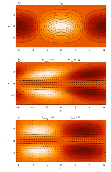
Figure 14.— Analytic solutions of the linearized shallow-water equations (16)–(18) in the limit of zero frictional drag. (a) shows the radiative-equilibrium height field. (b) and (c) show the solutions (height field in colorscale and velocity as arrows) for dimensionless $\tau_{\rm rad}$=10 and $\infty$, respectively.

Figure 14 illustrates the solutions for the case $\tilde{S}(y)=\hat{S}e^{-l^{2}y^{2}}$ with $l=0.6$ and $\hat{S}$ being a real constant. As in Figs. 2–3, the solutions exhibit midlatitude cyclones and anticyclones, with equatorial flow that is zonally aligned and diverges from a longitude near the substellar point. Because drag is zero, the layer is flat at the equator (see Eq. C4, which shows that $\eta=0$ for $y=0$). Interestingly, when $\tau_{\rm rad}$ is finite, the westward phase shift of the Rossby waves is large at low latitudes and approaches zero at high latitudes (Fig. 14b). This leads to phase tilts that are southwest-northeast in the northern hemisphere and northwest-southeast in the southern hemisphere—opposite to the cases shown in Figs. 2–3. In the limit $\tau_{\rm rad}\to\infty$, these phase tilts disappear and the solution strongly resembles that shown in the bottom right corner of Fig. 3.

Analysis of the continuity equation explains these behaviors. In addition to the mass source/sink caused by the forcing $S$, two processes affect the local layer thickness—radiative damping and horizontal convergence/divergence. Consider how their relative strengths depend on latitude. In the absence of drag, the linearized force balance is geostrophic, i.e., $yv=\partial\eta/\partial x$ and $yu=-\partial\eta/\partial y$ (see Eqs. 16–17). This means that, for a given velocity amplitude, the thickness gradients—and hence lateral thickness variations themselves—will be larger farther from the equator. As a result, for a given velocity amplitude, the radiative damping (which is $-\eta/\tau_{\rm rad}$) is stronger farther from the equator. On the other hand, in geostrophic balance, the wind flows parallel to contours of constant height, which severely limits the horizontal convergence/divergence; convergence can only come about due to variations of Coriolis parameter $f$ with latitude, which are stronger near the equator. In geostrophic balance, the horizontal divergence is $-\beta v/f$, which is just $-v/y$ for the equatorial beta plane considered here. Thus, for a given velocity amplitude, the amplitude of horizontal convergence is large near the equator but small at high latitudes. Given these latitude dependences, we thus expect that the thickness changes caused by the forcing ($S$) will predominantly be balanced by radiative relaxation at high latitude but horizontal convergence/divergence at low latitude.

Equations (C1–C2), which represent the zonal derivative of the continuity equation, describe exactly this balance. The three terms correspond to local changes in layer thickness due to the forcing $S$ (right side), mass source/sinks due to radiative damping (first term on left side), and changes in the layer thickness due to horizontal convergence or divergence of the fluid flow (second term on left side). For a given amplitude of $v$, the radiative damping increases with latitude (scaling with $y$), while the effect of horizontal convergence decreases with latitude (scaling with $y^{-1}$). The transition occurs at $y\sim\sqrt{k\tau_{\rm rad}}$ (or $y\sim\sqrt{gHk\tau_{\rm rad}/\beta}$ using dimensional quantities): radiative relaxation balances the forcing poleward of this latitude, whereas thickness changes due to horizontal convergence balance the forcing equatorward of this latitude.

When radiative relaxation balances the forcing ($y\gtrsim\sqrt{k\tau_{\rm rad}}$), the height field is in phase (in longitude) with the radiative equilibrium height field. When convergence/divergence balances the forcing ($y\lesssim\sqrt{k\tau_{\rm rad}}$), the convergence $\partial u/\partial x+\partial v/\partial y$, and therefore $v$ itself, are phase with the radiative-equilibrium height field. Since $\partial\eta/\partial x=yv$, this implies that the height field is phase shifted westward by $90^{\circ}$ relative to the radiative equilibrium height field. In the transition zone ($y\sim\sqrt{k\tau_{\rm rad}}$), these arguments imply that the phase lines of thickness—and therefore the velocities themselves—tilt from southwest-to-northeast in the northern hemisphere and northwest-to-southeast in the southern hemisphere. This explains the phase tilts seen in Fig. 14b. In the limit $\tau_{\rm rad}\to\infty$, the whole domain lies in the region where convergence balances forcing, explaining the lack of phase tilts of $\tilde{\eta}$ in Fig. 14c.

Appendix D D. Analytic solution in limit $\tau_{\rm rad}\to 0$

There also exist simple analytic solutions to the dimensionless, linearized shallow-water equations (16)–(18), for general $\tau_{\rm drag}$, in the limit $\tau_{\rm rad}\to 0$. This limit is particularly relevant for the hottest of tidally locked exoplanets, which, due to high temperature and/or significant visible-wavelength opacity, are expected to have short radiative time constants. Moreover, as a simplification of the full system it provides insights into the dynamical mechanisms.

In Appendix B, we showed that, in the limit $\tau_{\rm rad}\to 0$, the height field converges toward the radiative-equilibrium height field. Thus, in the momentum equations, we can replace the height with radiative-equilibrium height. The continuity equation involves the difference between $\eta$ and $\eta_{\rm eq}$, however, and so we must retain $\eta$ in that equation. This leads to the system:

$${\partial\eta_{\rm eq}\over\partial x}-yv=-{u\over\tau_{\rm drag}}$$ (D1)

$${\partial\eta_{\rm eq}\over\partial y}+yu=-{v\over\tau_{\rm drag}}$$ (D2)

$$\left({\partial u\over\partial x}+{\partial v\over\partial y}\right)={\eta_{\rm eq}-\eta\over\tau_{\rm rad}}$$ (D3)

Equations (D1)–(D2) constitute an algebraic system for $u$ and $v$ that can directly be solved to yield

$$u=-{{\partial\eta_{\rm eq}\over\partial x}+y\tau_{\rm drag}{\partial\eta_{\rm eq}\over\partial y}\over{1\over\tau_{\rm drag}}+y^{2}\tau_{\rm drag}}$$ (D4)

$$v={-{\partial\eta_{\rm eq}\over\partial y}+y\tau_{\rm drag}{\partial\eta_{\rm eq}\over\partial x}\over{1\over\tau_{\rm drag}}+y^{2}\tau_{\rm drag}}.$$ (D5)

Given $u$ and $v$, Eq. (D3) can then be solved to determine the (tiny) mismatch between $\eta$ and $\eta_{\rm eq}$.

Consider the limits of this solution for extreme values of the drag time constant. As $\tau_{\rm drag}\to 0$, Eqs. (D1)–(D2) imply that $u=-\tau_{\rm drag}^{-1}\partial\eta_{\rm eq}/\partial x$ and $v=-\tau_{\rm drag}^{-1}\partial\eta_{\rm eq}/\partial y$. In this strong-drag limit, the winds simply flow down the pressure gradient. On the other hand, in the limit of large $\tau_{\rm drag}$, then away from the equator, we obtain $u=-y^{-1}\partial\eta_{\rm eq}/\partial y$ and $v=y^{-1}\partial\eta_{\rm eq}\partial x$—implying geostrophic balance. Note that the approximate solutions (D4)–(D5) are singular at the equator in the limit $\tau_{\rm drag}\to\infty$; in this limit, the divergence becomes infinite at the equator, and the assumption that $\eta=\eta_{\rm eq}$ used to derive (D4)–(D5) no longer holds.

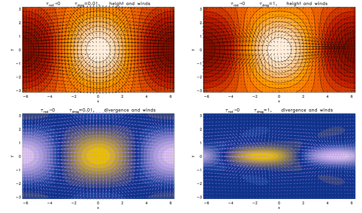
Figure 15.— Analytic solution of the linearized, dimensionless shallow-water equations on an equatorial beta plane (16)–(18) in the limit $\tau_{\rm rad}\to 0$. Left column shows solution for $\tau_{\rm drag}=0.01$, corresponding to the drag-dominated limit; the right column shows solution for $\tau_{\rm drag}=1$, implying that Coriolis and drag forces are comparable over much of the plotted region. In both cases, top panel shows winds and height field ($\equiv$radiative-equilibrium height field) and bottom panel shows divergence. The radiative-equilibrium heightfield is taken as $\eta_{\rm eq}=\eta_{\rm eq_{0}}e^{-l^{2}y^{2}}e^{ikx}$ with $l=0.316$ and $k=0.5$. For $\eta_{\rm eq_{0}}=0.8$, the maximum dimensionless wind speed is 0.0045 on the left and 0.45 on the right. The dimensionless divergence ranges between $-0.0036$ to $0.0036$ on the left and between $-0.54$ and $0.54$ on the right.

Figure 15 displays this solution for a drag-dominated case ($\tau_{\rm drag}=0.01$, left column) and case where drag is comparable to Coriolis forces over much of the domain ($\tau_{\rm drag}=1$, right column). The top row shows the winds with the assumed height field, and the bottom row shows the winds and the horizontal divergence. As expected, when drag is strong (left column), the air flows directly from the substellar point toward the antistellar point and is almost parallel to the pressure gradients. When drag is less dominant, however (right column), the solution forms a Matsuno-Gill-type wind pattern which exhibits velocities that tilt northwest-southeast in the northern hemisphere and southwest-northeast in the southern hemisphere. As discussed in §3, this pattern of velocity tilts would generate equatorial superrotation.

The mechanism for generating these velocity tilts is, simply, the three-way force balance between pressure-gradient, Coriolis, and drag forces. Because drag points in the opposite direction of the velocities, and Coriolis forces are perpendicular to the velocities, this three-way balance must give a velocity direction that is rotated clockwise of $-\nabla\eta$ in the northern hemisphere and counterclockwise of $-\nabla\eta$ in the southern hemisphere. A visual inspection of Fig. 15 makes clear that, given the expected pattern of $\nabla\eta_{\rm eq}$, this rotation forces the flow pattern to adopt velocity tilts that are northwest-southeast (southwest-northeast) in the northern (southern) hemisphere.

References

- Adcroft et al. (2004) Adcroft, A., Campin, J.-M., Hill, C., & Marshall, J. 2004, Monthly Weather Review, 132, 2845
- Agol et al. (2010) Agol, E., Cowan, N. B., Knutson, H. A., Deming, D., Steffen, J. H., Henry, G. W., & Charbonneau, D. 2010, ApJ, 721, 1861
- Andrews et al. (1987) Andrews, D. G., Holton, J. R., & Leovy, C. B. 1987, Middle Atmosphere Dynamics (Academic Press, New York)
- Batalha et al. (2011) Batalha, N. M., Borucki, W. J., Bryson, S. T., Buchhave, L. A., Caldwell, D. A., Christensen-Dalsgaard, J., Ciardi, D., Dunham, E. W., Fressin, F., Gautier, III, T. N., Gilliland, R. L., Haas, M. R., Howell, S. B., Jenkins, J. M., Kjeldsen, H., Koch, D. G., Latham, D. W., Lissauer, J. J., Marcy, G. W., Rowe, J. F., Sasselov, D. D., Seager, S., Steffen, J. H., Torres, G., Basri, G. S., Brown, T. M., Charbonneau, D., Christiansen, J., Clarke, B., Cochran, W. D., Dupree, A., Fabrycky, D. C., Fischer, D., Ford, E. B., Fortney, J., Girouard, F. R., Holman, M. J., Johnson, J., Isaacson, H., Klaus, T. C., Machalek, P., Moorehead, A. V., Morehead, R. C., Ragozzine, D., Tenenbaum, P., Twicken, J., Quinn, S., VanCleve, J., Walkowicz, L. M., Welsh, W. F., Devore, E., & Gould, A. 2011, ArXiv e-prints
- Bean et al. (2010) Bean, J. L., Kempton, E., & Homeier, D. 2010, Nature, 468, 669
- Borucki et al. (2011) Borucki, W. J., Koch, D. G., Basri, G., Batalha, N., Brown, T. M., Bryson, S. T., Caldwell, D., Christensen-Dalsgaard, J., Cochran, W. D., DeVore, E., Dunham, E. W., Gautier, III, T. N., Geary, J. C., Gilliland, R., Gould, A., Howell, S. B., Jenkins, J. M., Latham, D. W., Lissauer, J. J., Marcy, G. W., Rowe, J., Sasselov, D., Boss, A., Charbonneau, D., Ciardi, D., Doyle, L., Dupree, A. K., Ford, E. B., Fortney, J., Holman, M. J., Seager, S., Steffen, J. H., Tarter, J., Welsh, W. F., Allen, C., Buchhave, L. A., Christiansen, J. L., Clarke, B. D., Désert, J., Endl, M., Fabrycky, D., Fressin, F., Haas, M., Horch, E., Howard, A., Isaacson, H., Kjeldsen, H., Kolodziejczak, J., Kulesa, C., Li, J., Machalek, P., McCarthy, D., MacQueen, P., Meibom, S., Miquel, T., Prsa, A., Quinn, S. N., Quintana, E. V., Ragozzine, D., Sherry, W., Shporer, A., Tenenbaum, P., Torres, G., Twicken, J. D., Van Cleve, J., & Walkowicz, L. 2011, ArXiv e-prints
- Charbonneau et al. (2009) Charbonneau, D., Berta, Z. K., Irwin, J., Burke, C. J., Nutzman, P., Buchhave, L. A., Lovis, C., Bonfils, X., Latham, D. W., Udry, S., Murray-Clay, R. A., Holman, M. J., Falco, E. E., Winn, J. N., Queloz, D., Pepe, F., Mayor, M., Delfosse, X., & Forveille, T. 2009, Nature, 462, 891
- Charbonneau et al. (2008) Charbonneau, D., Knutson, H. A., Barman, T., Allen, L. E., Mayor, M., Megeath, S. T., Queloz, D., & Udry, S. 2008, ApJ, 686, 1341
- Cooper & Showman (2005) Cooper, C. S., & Showman, A. P. 2005, ApJ, 629, L45
- Cooper & Showman (2006) —. 2006, ApJ, 649, 1048
- Cowan et al. (2007) Cowan, N. B., Agol, E., & Charbonneau, D. 2007, MNRAS, 379, 641
- Crossfield et al. (2010) Crossfield, I. J. M., Hansen, B. M. S., Harrington, J., Cho, J., Deming, D., Menou, K., & Seager, S. 2010, ApJ, 723, 1436
- Del Genio & Zhou (1996) Del Genio, A. D., & Zhou, W. 1996, Icarus, 120, 332
- Del Genio et al. (1993) Del Genio, A. D., Zhou, W., & Eichler, T. P. 1993, Icarus, 101, 1
- Dobbs-Dixon et al. (2010) Dobbs-Dixon, I., Cumming, A., & Lin, D. N. C. 2010, ApJ, 710, 1395
- Dobbs-Dixon & Lin (2008) Dobbs-Dixon, I., & Lin, D. N. C. 2008, ApJ, 673, 513
- Gill (1980) Gill, A. E. 1980, Q. J. Roy. Meteor. Soc., 106, 447
- Hack & Jakob (1992) Hack, J. J., & Jakob, R. 1992, Description of a global shallow water model based on the spectral transform method, Tech. rep., National Center for Atmospheric Research Technical note NCAR/TN-343+STR, Boulder, CO
- Harrington et al. (2006) Harrington, J., Hansen, B. M., Luszcz, S. H., Seager, S., Deming, D., Menou, K., Cho, J. Y.-K., & Richardson, L. J. 2006, Science, 314, 623
- Held (1999) Held, I. M. 1999, Bernhard Haurwitz Memorial Lecture, American Meteorological Society, available at www.gfdl.noaa.gov/isaac
- Held (2000) —. 2000, Paper presented at 2000 Woods Hole Oceanographic Institute Geophysical Fluid Dynamics Program, Woods Hole Oceanographic Institute, Woods Hole, MA (available at http://www.whoi.edu/page.do?pid=13076)
- Held & Hou (1980) Held, I. M., & Hou, A. Y. 1980, Journal of Atmospheric Sciences, 37, 515
- Heng et al. (2010) Heng, K., Menou, K., & Phillipps, P. J. 2010, ArXiv e-prints
- Heng & Vogt (2010) Heng, K., & Vogt, S. S. 2010, ArXiv e-prints
- Hide (1969) Hide, R. 1969, J. Atmos. Sci., 26, 841
- Holton (2004) Holton, J. R. 2004, An Introduction to Dynamic Meteorology, 4th Ed. (Academic Press, San Diego)
- Joshi (2003) Joshi, M. 2003, Astrobiology, 3, 415
- Joshi et al. (1997) Joshi, M. M., Haberle, R. M., & Reynolds, R. T. 1997, Icarus, 129, 450
- Knutson et al. (2007) Knutson, H. A., Charbonneau, D., Allen, L. E., Fortney, J. J., Agol, E., Cowan, N. B., Showman, A. P., Cooper, C. S., & Megeath, S. T. 2007, Nature, 447, 183
- Knutson et al. (2009) Knutson, H. A., Charbonneau, D., Cowan, N. B., Fortney, J. J., Showman, A. P., Agol, E., Henry, G. W., Everett, M. E., & Allen, L. E. 2009, ApJ, 690, 822
- Koskinen et al. (2007) Koskinen, T. T., Aylward, A. D., Smith, C. G. A., & Miller, S. 2007, ApJ, 661, 515
- Kraucunas & Hartmann (2005) Kraucunas, I., & Hartmann, D. L. 2005, J. Atmos. Sci., 62, 371
- Léger et al. (2009) Léger, A., Rouan, D., Schneider, J., Barge, P., Fridlund, M., Samuel, B., Ollivier, M., Guenther, E., Deleuil, M., Deeg, H. J., Auvergne, M., Alonso, R., Aigrain, S., Alapini, A., Almenara, J. M., Baglin, A., Barbieri, M., Bruntt, H., Bordé, P., Bouchy, F., Cabrera, J., Catala, C., Carone, L., Carpano, S., Csizmadia, S., Dvorak, R., Erikson, A., Ferraz-Mello, S., Foing, B., Fressin, F., Gandolfi, D., Gillon, M., Gondoin, P., Grasset, O., Guillot, T., Hatzes, A., Hébrard, G., Jorda, L., Lammer, H., Llebaria, A., Loeillet, B., Mayor, M., Mazeh, T., Moutou, C., Pätzold, M., Pont, F., Queloz, D., Rauer, H., Renner, S., Samadi, R., Shporer, A., Sotin, C., Tingley, B., Wuchterl, G., Adda, M., Agogu, P., Appourchaux, T., Ballans, H., Baron, P., Beaufort, T., Bellenger, R., Berlin, R., Bernardi, P., Blouin, D., Baudin, F., Bodin, P., Boisnard, L., Boit, L., Bonneau, F., Borzeix, S., Briet, R., Buey, J., Butler, B., Cailleau, D., Cautain, R., Chabaud, P., Chaintreuil, S., Chiavassa, F., Costes, V., Cuna Parrho, V., de Oliveira Fialho, F., Decaudin, M., Defise, J., Djalal, S., Epstein, G., Exil, G., Fauré, C., Fenouillet, T., Gaboriaud, A., Gallic, A., Gamet, P., Gavalda, P., Grolleau, E., Gruneisen, R., Gueguen, L., Guis, V., Guivarc’h, V., Guterman, P., Hallouard, D., Hasiba, J., Heuripeau, F., Huntzinger, G., Hustaix, H., Imad, C., Imbert, C., Johlander, B., Jouret, M., Journoud, P., Karioty, F., Kerjean, L., Lafaille, V., Lafond, L., Lam-Trong, T., Landiech, P., Lapeyrere, V., Larqué, T., Laudet, P., Lautier, N., Lecann, H., Lefevre, L., Leruyet, B., Levacher, P., Magnan, A., Mazy, E., Mertens, F., Mesnager, J., Meunier, J., Michel, J., Monjoin, W., Naudet, D., Nguyen-Kim, K., Orcesi, J., Ottacher, H., Perez, R., Peter, G., Plasson, P., Plesseria, J., Pontet, B., Pradines, A., Quentin, C., Reynaud, J., Rolland, G., Rollenhagen, F., Romagnan, R., Russ, N., Schmidt, R., Schwartz, N., Sebbag, I., Sedes, G., Smit, H., Steller, M. B., Sunter, W., Surace, C., Tello, M., Tiphène, D., Toulouse, P., Ulmer, B., Vandermarcq, O., Vergnault, E., Vuillemin, A., & Zanatta, P. 2009, A&A, 506, 287
- Lewis et al. (2010) Lewis, N. K., Showman, A. P., Fortney, J. J., Marley, M. S., Freedman, R. S., & Lodders, K. 2010, ApJ, 720, 344
- Li & Goodman (2010) Li, J., & Goodman, J. 2010, ArXiv e-prints
- Lian & Showman (2008) Lian, Y., & Showman, A. P. 2008, Icarus, 194, 597
- Lian & Showman (2010) —. 2010, Icarus, 207, 373
- Lindzen (1981) Lindzen, R. S. 1981, J. Geophys. Res., 86, 9707
- Marley & McKay (1999) Marley, M. S., & McKay, C. P. 1999, Icarus, 138, 268
- Matsuno (1966) Matsuno, T. 1966, J. Meteorol. Soc. Japan, 44, 25
- Menou & Rauscher (2009) Menou, K., & Rauscher, E. 2009, ApJ, 700, 887
- Merlis & Schneider (2010) Merlis, T. M., & Schneider, T. 2010, ArXiv e-prints
- Mitchell & Vallis (2010) Mitchell, J. L., & Vallis, G. K. 2010, ArXiv e-prints
- Norton (2006) Norton, W. A. 2006, J. Atmos. Sci., 63, 1420
- O’Gorman & Schneider (2007) O’Gorman, P. A., & Schneider, T. 2007, Geophys. Res. Lett., 34, 22801
- Pedlosky (1987) Pedlosky, J. 1987, Geophysical Fluid Dynamics, 2nd Ed. (Springer-Verlag, New York)
- Perna et al. (2010) Perna, R., Menou, K., & Rauscher, E. 2010, ApJ, 719, 1421
- Rauscher & Menou (2010) Rauscher, E., & Menou, K. 2010, ApJ, 714, 1334
- Saravanan (1993) Saravanan, R. 1993, J. Atmos. Sci., 50, 1211
- Sardeshmukh & Hoskins (1985) Sardeshmukh, P. D., & Hoskins, B. J. 1985, Quarterly Journal of the Royal Meteorological Society, 111, 261
- Sardeshmukh & Hoskins (1988) —. 1988, Journal of Atmospheric Sciences, 45, 1228
- Schneider & Liu (2009) Schneider, T., & Liu, J. 2009, J. Atmos. Sci., 66, 579
- Shell & Held (2004) Shell, K. M., & Held, I. M. 2004, J. Atmos. Sci., 61, 2928
- Showman et al. (2008) Showman, A. P., Cooper, C. S., Fortney, J. J., & Marley, M. S. 2008, ApJ, 682, 559
- Showman et al. (2009) Showman, A. P., Fortney, J. J., Lian, Y., Marley, M. S., Freedman, R. S., Knutson, H. A., & Charbonneau, D. 2009, ApJ, 699, 564
- Showman & Guillot (2002) Showman, A. P., & Guillot, T. 2002, A&A, 385, 166
- Showman & Polvani (2010) Showman, A. P., & Polvani, L. M. 2010, Geophys. Res. Lett., in press
- Showman et al. (2010) Showman, A. P., Y-K. Cho, J., & Menou, K. 2010, ArXiv e-prints
- Suarez & Duffy (1992) Suarez, M. J., & Duffy, D. G. 1992, J. Atmos. Sci., 49, 1541
- Swain et al. (2009) Swain, M. R., Vasisht, G., Tinetti, G., Bouwman, J., Chen, P., Yung, Y., Deming, D., & Deroo, P. 2009, ApJ, 690, L114
- Thompson (1971) Thompson, R. O. R. Y. 1971, Journal of Physical Oceanography, 1, 235
- Thrastarson & Cho (2010) Thrastarson, H. T., & Cho, J. 2010, ApJ, 716, 144
- Thuburn & Lagneau (1999) Thuburn, J., & Lagneau, V. 1999, J. Atmos. Sci., 56, 689
- Vallis (2006) Vallis, G. K. 2006, Atmospheric and Oceanic Fluid Dynamics: Fundamentals and Large-Scale Circulation (Cambridge Univ. Press, Cambridge, UK)
- Watkins & Cho (2010) Watkins, C., & Cho, J. 2010, ApJ
- Williams (2003a) Williams, G. P. 2003a, Journal of Atmospheric Sciences, 60, 2136
- Williams (2003b) —. 2003b, Journal of Atmospheric Sciences, 60, 1270
- Wu et al. (2001) Wu, Z., Sarachik, E. S., & Battisti, D. S. 2001, J. Atmos. Sci., 58, 724