Berry phase of non-ideal Dirac fermions in topological insulators

Abstract

A distinguishing feature of Dirac fermions is the Berry phase of $\pi$ associated with their cyclotron motions. Since this Berry phase can be experimentally assessed by analyzing the Landau-level fan diagram of the Shubnikov-de Haas (SdH) oscillations, such an analysis is widely employed in recent transport studies of topological insulators to elucidate the Dirac nature of the surface states. However, the reported results have usually been unconvincing. Here we show a general scheme for describing the phase factor of the SdH oscillations in realistic surface states of topological insulators, and demonstrate how one could elucidate the Dirac nature in the real experimental data.

I Introduction

During the last three decades, the Berry phase Berry has become an important concept in condensed matter physics, S-W playing a fundamental role in various phenomena such as electric polarization, orbital magnetism, anomalous Hall effects, etc. Niu2010 The Berry phase (or geometrical phase) in solids is determined by topological characteristics of the energy bands in the Brillouin zone (BZ) and represents a fundamental property of the system. For example, a non-zero Berry phase, which can be measured directly in the magnetotransport experiments, reflects the existence of a singularity in the energy bands such as a band-contact line in three-dimensional (3D) bulk states or a Dirac point in a two-dimensional (2D) surface state. Mikitik1999 Also, the Berry phase of $\pi$ is responsible for the peculiar “anti-localization” effects in carbon nanotubes or graphene. TAndo Recently, the $\pi$ Berry phase has been observed in the Shubnikov-de Haas (SdH) oscillations in graphene, N-G2005 ; Kim2005 giving one of the key evidences for the Dirac nature of quasiparticles in the 2D carbon sheet.

The 3D topological insulator (TI) also supports spin polarized 2D Dirac fermions on its surface,HK which can be distinguished from ordinary charge carriers by a non-zero Berry phase. Recently, several groups have reported observations of the SdH oscillations coming from the 2D surface states of TIs. BiSb_amro ; Ong2010 ; Fisher_np ; BTS_Rapid ; Xiong ; Morpurgo ; HgTe ; Bi2Te3nano In those studies, a finite Berry phase has been reported, but it usually deviates from the exact $\pi$ value. For example, in the new TI material Bi₂Te₂Se (BTS), BTS_Rapid where a large contribution of the surface transport to the total conductivity has been observed, the apparent Berry phase extracted from the SdH-oscillation data was 0.44$\pi$. So far, the Zeeman coupling of the spin to the magnetic field has been considered Fisher_np as a possible source of such a discrepancy. Here, we show that in addition to the Zeeman term, the deviation of the dispersion relation $E(k)$ from an ideal linear dispersion DasSarma2010 can shift the Berry phase from $\pi$. We further show how the real experimental data for non-ideal Dirac fermions could be understood by taking into account those additional factors.

II energy dispersion of surface states

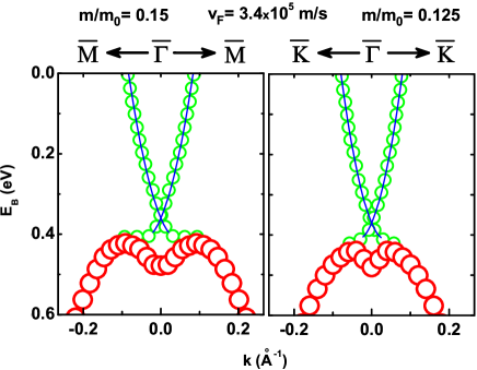
Figure 1: (Color online) Experimental band dispersions (symbols) in Bi₂Te₂Se measured by ARPES in Ref. BTS_Hasan, and the fitting of Eq. (1) to the surface state (solid line). Large symbols depict the bulk state.

The energy dispersion of the surface states in TIs can be directly measured in angle-resolved photoemission spectroscopy (ARPES) experiments. As an example, Fig. 1 shows the dispersion of the surface state (together with the bulk state) in BTS reported by Xu et al. BTS_Hasan One can easily recognize that $E(k)$ is not an ideal Dirac-like dispersion, but it can be fitted reasonably well for the two high-symmetry axes with

$$E(k)=v_{F}\hbar\,k+\frac{\hbar^{2}}{2m}k^{2},$$ (1)

with a single Fermi velocity $v_{F}$ = 3.4$\times$10⁵ m/s and the effective mass $m$ which slightly varies with the direction in the surface BZ as shown by the solid lines in Fig. 1 [$m/m_{0}$ = 0.15 (0.125) for the $\bar{\Gamma}\rightarrow\bar{M}$ ($\bar{\Gamma}\rightarrow\bar{K}$) direction with $m_{0}$ the free electron mass].

Similar fittings can be obtained for other TIs owing to the progress in the ARPES studies of these materials. HK ; HgTe ; H5 ; Chen

III Berry phase in quantum oscillations

It is commonly accepted that quantum oscillations observed in 3D metals can be well understood within Lifshits-Kosevich L-K (the de Haas-van Alphen effect) and Adams-Holstein A-H (the SdH effect) theories. Recently this approach has been generalized to describe magnetic oscillations in graphene, which is a 2D system with a Dirac-like spectrum of charge carriers. Sh-G-B ; G-Sh There are two most prominent features that distinguish such systems from materials with a parabolic spectrum: First, rather weak magnetic fields are sufficient to bring the system into a regime where only a few Landau levels are occupied. Second, Dirac quasiparticles acquire the Berry phase of $\pi$ in the cyclotron motion, changing the phase of quantum oscillations.

In the SdH effect, the oscillating part of $\rho_{xx}$ follows

$$\Delta\rho_{xx}\sim\cos[2\pi(\frac{F}{B}-\gamma)],$$ (2)

where $F$ is the oscillation frequency and 2$\pi\gamma$ is the phase factor ($0\leq\gamma<1$). This is the same $\gamma$ as in the Onsager’s semiclassical quantization condition Shoenberg1984

$$A_{N}=\frac{2\pi e}{\hbar}B(N+\gamma),$$ (3)

when the $N$-th Landau level (LL) is crossing the Fermi energy $E_{F}$ ($A_{N}$ is the area of an electron orbit in the $k$-space). $\gamma$ is directly related to the Berry phase throughMikitik1999

$$\gamma-\frac{1}{2}=-\frac{1}{2\pi}\oint_{\Gamma}\vec{\Omega}\,d\vec{k},$$ (4)

where $\vec{\Omega}(\vec{k})$=i$\int d\vec{k}\,u_{\vec{k}}^{*}(\vec{r})\,\vec{\nabla}_{\vec{k}}u_{\vec{k}}(\vec{r})$ is the Berry connection, $u_{\vec{k}}(\vec{r})$ is the amplitude of the Bloch wave function, $\Gamma$ is a closed electron orbit (the intersection of the Fermi surface $E(\vec{k})=E_{F}$ with the plane $k_{z}=const$). For spinless quasiparticles, it is known Mikitik1999 ; Shoenberg1984 that the Berry phase is zero for a parabolic energy dispersion ($\gamma$ = $\frac{1}{2}$) and $\pi$ for a linear energy dispersion ($\gamma$ = 0).

Experimentally, $\gamma$ can be obtained from an analysis of the Landau-level (LL) fan diagram. There are three quantities which are often used as abscissa for plotting a LL fan diagram: (i) Landau level index $N$, which determines the energy $E_{N}$ of the $N$-th LL. (ii) Filling factor $\nu$ ($\equiv\frac{N_{s}S}{N_{\phi}}$, where $N_{s}$ is the density of charge carriers, $S$ is the area of the sample, $N_{\phi}$ = $\frac{BS}{\Phi_{0}}$ is the number of flux quanta, and $\Phi_{0}$=$\frac{h}{e}$ is the flux quantum). (iii) An integer number $n$ which marks the $n$-th minimum of the oscillations in $\rho_{xx}$. Although all three quantities are related to each other, the most straightforward way to plot a LL fan diagram from the $\rho_{xx}$ oscillations in a 2D system Ong2010 is to assign an integer $n$ to a minimum of $\rho_{xx}$ (or a half-integer to a maximum of $\rho_{xx}$). From Eq. (2), one can see that the first minimum in $\rho_{xx}$ is always in the range of $0<\frac{F}{B_{1}}\leq 1$. Thus, the plot of $F/B_{n}$ vs $n$, which makes a straight line with a unit slope for periodic oscillations, is uniquely defined and cuts the $n$-axis between 0 and 1 depending on the phase of the oscillations, $\gamma$.

The ordinate 1/$B_{n}$ in a LL fan diagram is determined by the Landau quantization of the cyclotron motion of electrons in a magnetic field. In 2D systems, upon sweeping $B$, $\rho_{xx}$ shows a maximum (or a sharp peak in the quantum Hall effect Ong2010 ) each time when $E_{N}(B)$ crosses the Fermi level. Thus, the position of the maximum in $\rho_{xx}$ that corresponds to the $N$-th LL, 1/$B_{N}$, is given by

$$2\pi\Big{(}\frac{F}{B_{N}}-\gamma\Big{)}=2\pi N.$$ (5)

On the other hand, the $n$-th minimum in $\rho_{xx}$ occurs at 1/$B_{n}$ when $2\pi(\frac{F}{B_{n}}-\gamma)=2\pi n-\pi$, so the positions of the maxima and minima are shifted by $\frac{1}{2}$ on the $n$-axis.

The Onsager’s relation Shoenberg1984 gives $F$ in terms of the Fermi wave vector $k_{F}$ as $F=(\hbar/2\pi e)\pi k_{F}^{2}$, and this $k_{F}$ can be calculated from Eq. (1) as

$$k_{F}^{2}=2\Big{(}\frac{mv_{F}}{\hbar}\Big{)}^{2}\Bigg{(}1+\frac{E_{F}}{mv_{F}^{2}}-\sqrt{1+\frac{2E_{F}}{mv_{F}^{2}}}\Bigg{)}.$$ (6)

Also, when $E_{F}$ is at the $N$-th LL, there is a relation

$$E_{N}(B_{N})=E_{F}.$$ (7)

From Eqs. (5)–(7), one obtains

$$\gamma=\frac{mv_{F}^{2}}{\hbar\,\omega_{c}}\Bigg{(}1+\frac{E_{N}}{mv_{F}^{2}}-\sqrt{1+\frac{2E_{N}}{mv_{F}^{2}}}\Bigg{)}-N,$$ (8)

where $\omega_{c}$=$eB/m$ is the cyclotron frequency.

In general case, $\gamma$ is a function of $B$, meaning that oscillations in $\rho_{xx}$ are quasi-periodic in $1/B$. In order to calculate $\gamma$ one needs to find the eigenvalues $E_{N}$ for a given Hamiltonian.

IV Model Hamiltonian

For the (111) surface state of the Bi₂Se₃-family TI compounds, the Hamiltonian for non-ideal Dirac quasiparticles in perpendicular magnetic fields can be written as MQOsc

$$\hat{H}=v_{F}(\Pi_{x}\sigma_{y}-\Pi_{y}\sigma_{x})+\frac{{\bf\Pi}^{2}}{2m}-\frac{1}{2}\,g_{s}\mu_{B}B\sigma_{z},$$ (9)

where the Landau gauge ${\bf A}=(0,By,0)$ for the vector potential is used, ${\bf\Pi}$=$\hbar\,{\bf k}$+$e{\bf A}$, $\sigma_{i}$ are the Pauli matrices, $\mu_{B}$ is the Bohr magneton, and $g_{s}$ is the surface $g$-factor. The LL energies are given by MQOsc ; PP2009

$$E_{N}^{(\pm)}=\hbar\omega_{c}N\pm\sqrt{2\hbar\,v_{F}^{2}eBN+\Big{(}\frac{1}{2}\hbar\omega_{c}-\frac{1}{2}\,g_{s}\mu_{B}B\Big{)}^{2}},$$ (10)

where “$+$” and “$-$” branches are for electrons and holes, respectively. The obtained eigenvalues $E_{N}$ define the exact positions of maxima in $\rho_{xx}$ and, thus, the phase of oscillations through Eq. (8).

In two extreme cases, for non-magnetic fermions ($g_{s}$ = 0), Eq. (8) gives the expected results. First, for a linear dispersion (ideal Dirac fermions), $m\rightarrow\infty$ leads to $E_{N}$=$\pm\sqrt{2\hbar\,ev_{F}^{2}BN}$ and $\gamma\rightarrow\frac{E_{N}^{2}}{2\hbar\,ev_{F}^{2}B}-N$, giving $\gamma$ = 0 (Berry phase is $\pi$). Second, for a parabolic dispersion, $v_{F}\rightarrow$ 0 leads to $E_{N}$=$\hbar\,\omega_{c}(N+\frac{1}{2})$ and $\gamma\rightarrow\frac{E_{N}}{\hbar\,\omega_{c}}-N$, giving $\gamma$ = $\frac{1}{2}$ (Berry phase is zero). This gives confidence that the expression for $\gamma$ given in Eq. (8) is generally valid for the topological surface state with a non-ideal Dirac cone described by Eq. (1).

V Landau-level fan diagram for non-ideal Dirac fermions

Figure 2: (Color online) (a) Landau level fan diagram calculated for $F$ = 60 T, $v_{F}$ = 3$\times$10⁵ m/s, $g_{s}$ = 0, and different $m/m_{0}$. Arrows show the direction of decreasing $m/m_{0}$. The dashed and dotted lines are the expected behaviors for an ideal Dirac dispersion and a parabolic dispersion, respectively. (b) Landau level fan diagram calculated for $F$ = 60 T, $m/m_{0}$ = 0.1, $g_{s}$ = 0, and different $v_{F}$. Arrows show the direction of decreasing $v_{F}$. Insets show the calculated $\gamma(N)$.

Let us first consider how the LL fan diagram will be modified, when both linear and parabolic terms are present in the Hamiltonian [Eq. (9)]. For the moment, the Zeeman coupling of the electron spin to the magnetic field is assumed to be negligible ($g_{s}$ = 0). Figure 2 (a) shows the calculated positions of maxima and minima in $\rho_{xx}$ for oscillations with $F$ = 60 T and $v_{F}$ = 3$\times$10⁵ m/s as $m/m_{0}$ is varied. One can see that upon decreasing $m/m_{0}$, the calculated lines on the LL fan diagram are gradually shifting upward from the ideal Dirac line that crosses the $n$-axis at exactly $\frac{1}{2}$. Moreover, the lines are not straight anymore, which is clearly inferred in the dependence of $\gamma$ vs $N$ shown in the inset. With decreasing $N$ (increasing $B$), $\gamma$ becomes larger, reflecting the change in the phase of oscillations at high fields.

Similar change in the LL fan diagram occurs if we modify another parameter, $v_{F}$. As shown in Fig. 2 (b), the calculated lines are gradually shifting upward from the ideal Dirac line as $v_{F}$ is decreased. The results shown in Figs. 2 can be understood as a competition between linear and quadratic terms in the Hamiltonian [Eq. (9)]. Note that for the whole range of the parameters $v_{F}$ and $m/m_{0}$, the positions of maxima and minima in $\rho_{xx}$ lie between two straight lines (shown as dotted and dashed lines in Figs. 2) corresponding to $\gamma$ = 0 and $\gamma$ = $\frac{1}{2}$.

Figure 3: (Color online) Landau level fan diagram calculated for $F$ = 60 T and different $g_{s}$, keeping $v_{F}$ = 3$\times$10⁵ m/s and $m/m_{0}$ = 0.1 constant. Arrows show the direction of changing $g_{s}$. The dotted line is the expected behavior for a parabolic dispersion. Inset shows the calculated $\gamma(N)$.

Let us now take the Zeeman term into considerations. Figure 3 shows the LL fan diagram calculated with $F$ = 60 T, $v_{F}$ = 3$\times$10⁵ m/s, and $m/m_{0}$ = 0.1, while $g_{s}$ is varied. To understand the effect of the Zeeman coupling, it is important to recognize the following two points: (i) The Zeeman term in Eq. (10) would tend to cancel the $\frac{1}{2}\hbar\omega_{c}$ term when $g_{s}$ is positive. In fact, when $\frac{1}{2}\hbar\omega_{c}$ = $\frac{1}{2}g_{s}\mu_{B}B$ (i.e., $g_{s}=2m_{0}/m$) is satisfied, the effect of the finite effective mass is canceled and the LL fan diagram becomes identical to that for the linear dispersion (ideal Dirac) case. In the present simulations, we use $m/m_{0}$ = 0.1, so that this cancellations occurs when $g_{s}$ = 20. (ii) A pair of $g_{s}$ values that give the same $|\frac{1}{2}\hbar\omega_{c}-\frac{1}{2}g_{s}\mu_{B}B|$ are effectively the same in determining the behavior of the LL fan diagram. The result of our calculations shown in Fig. 3 is a demonstration of these two points. Since the Zeeman effect is more pronounced at higher fields, the LL fan diagram in Fig. 3 is strongly modified from a straight line when the quantum limit is approached, i.e., close to $N$ = 0.

VI The case of BTS

Figure 4: (Color online) Landau level fan diagram for oscillations in $d\rho_{xx}/dB$ measured at $T$ = 1.6 K and $\theta\simeq$ 0^∘ reported in Ref. BTS_Rapid, for BTS. Minima and maxima in $d\rho_{xx}/dB$ correspond to $n+\frac{1}{4}$ and $n+\frac{3}{4}$, respectively. Solid (dark gray) line is the calculated diagram for an ideal Dirac cone with $v_{F}$ = 3.4$\times$10⁵ m/s and $F$ = 62 T; dashed (blue) line includes the effect of the actual dispersion with $m/m_{0}$ = 0.13; dotted (red) line further includes the Zeeman effect, where $g_{s}$ = 76 or $-45$ was determined from a least-square fitting to the data. Inset shows the experimental data and calculations after subtracting the contribution from an ideal Dirac cone, $(1/B)_{\rm Dirac}$, where $\Delta(1/B)\equiv(1/B)-(1/B)_{\rm Dirac}$.

Let us examine the real data measured in the BTS sample, BTS_Rapid in the light of the above considerations. Figure 4 shows the LL fan diagram for oscillations in $d\rho_{xx}/dB$ measured at $T$ = 1.6 K in magnetic fields perpendicular to the (111) plane. BTS_Rapid In Ref. BTS_Rapid, , the data were simply fitted with a straight line, and the least-square fitting gave a slope of $F$ = 64 T with the intersection of the $n$-axis at 0.22$\pm$0.12; this result implies a finite Berry phase, but it was not exactly equal to $\pi$, which remained a puzzle. BTS_Rapid Now, we analyze this LL fan diagram by considering the non-ideal Dirac dispersion as well as the Zeeman effect. The ARPES data BTS_Hasan for the surface state of BTS (Fig. 1) gives $v_{F}$ = 3.4$\times$10⁵ m/s and the averaged effective mass $m/m_{0}$ = 0.13. We fix the oscillation frequency $F$ at 62 T obtained from the Fourier-transform analysis of the $d\rho_{xx}/dB$ oscillations.BTS_Rapid

In Fig. 4, the calculated diagram for an ideal Dirac cone is shown by the solid (dark gray) line, whereas that for the non-ideal Dirac cone with the effective-mass term is shown by the dashed (blue) line. One can see that the difference is small, which indicates that the effective mass of 0.13$m_{0}$ is not light enough to significantly alter the LL fan diagram. One may also see that these two lines undershoot the actual data points at smaller $n$, which is even more clearly seen in the inset, where the experimental data and the calculations are shown after subtracting the contribution from an ideal Dirac cone. By further including the Zeeman effect, we can greatly improve the analysis, as shown by the dotted (red) line; here, $g_{s}$ is taken as the only fitting parameter and a least-square fitting to the data was performed. The best value of $g_{s}$ is 76 or $-45$.

The inset of Fig. 4 makes it clear that it is the slight deviation of the experimental points from the ideal Dirac line that causes a simple straight-line fitting of the LL fan diagram to intersect the $n$-axis not exactly at 0.5. Since the Berry phase in real situations is not a fixed value but is dependent on the magnetic field, the simple straight-line analysis of the LL fan diagram should not be employed for the determination of the Berry phase. Obviously, the SdH oscillations of the topological surface states are best understood by the analysis which considers both the the deviation of the energy spectrum of the Dirac-like charge carriers from the ideal linear dispersion and their strong coupling with an external magnetic field.

VII Other materials

Material	$v_{F}$ (m/s)	$m/m_{0}$	Ref.	remark
Bi2Se3	3.0 $\times$105	0.25	[H5, ]	averaged
Bi2Te2Se	3.4 $\times$105	0.13	[BTS_Rapid, ]	averaged
Bi2Te3	3.7 $\times$105	3.8	[Chen, ]	near Dirac point
graphene	1 $\times$106	$\infty$	[N-G2005, ]	calculations

Table 1: Parameters of the surface states from ARPES.

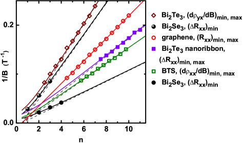
Figure 5: (Color online) Landau level fan diagrams for SdH oscillations observed in various TIs and graphene. Symbols are obtained from the published experimental data in the literature. Solid lines are calculations taking into account the non-ideal dispersions of the surface states (determined by $m/m_{0}$) and the Zeeman coupling to an external magnetic field (determined by $g_{s}$). Dashed lines are calculations for ideal Dirac fermions ($m/m_{0}$ = $\infty$ and $g_{s}$ = 0). Open diamonds are $(d\rho_{yx}/dB)_{min,max}$ in Bi₂Te₃ from Ref. Ong2010, ; filled circles are $(\Delta R_{xx})_{min}$ in Bi₂Se₃ from Ref. Fisher_np, ; open circles are $(R_{xx})_{min,max}$ in graphene from Ref. N-G2005, ; filled squares are $(\Delta R_{xx})_{min,max}$ in a Bi₂Te₃ nanoribbon from Ref. Bi2Te3nano, ; open squares are $(d\rho_{xx}/dB)_{min,max}$ in BTS from Ref. BTS_Rapid, .

Similar analysis can be performed for other TIs in which the quantum oscillations coming from the 2D topological surface states have been observed. Figure 5 shows the LL fan diagrams for the SdH oscillations published to date for TI materials, Fisher_np ; Ong2010 ; BTS_Rapid ; Bi2Te3nano ; note1 together with the data obtained in graphene, N-G2005 which provides a good reference for studies of Dirac fermions. We digitized the published experimental data in the literature and determined ourselves the positions of minima $1/B_{min}$ and maxima $1/B_{max}$ of the oscillating parts of resistivity (resistance), Hall resistivity, or their derivatives with respect to $B$. The obtained data for various materials are plotted as functions of $n$ in Fig. 5. Note that, to avoid ambiguities, we considered only those data that show oscillations with a single frequency. note1

Material	Ref.	$F$ (T)	$E_{F}$ (eV)	$g_{s}$
Bi2Se3	[Fisher_np, ]	30.7	0.074	55 or -39
Bi2Se3	[Fisher_np, ]	88.6	0.143	55 or -39
Bi2Te2Se	[BTS_Rapid, ]	62.0	0.152	76 or -45
Bi2Te3	[Ong2010, ]	27.3	0.074	65 or -65
Bi2Te3, nanoribbon	[Bi2Te3nano, ]	54.7	0.101	65 or -65
graphene	[N-G2005, ]	43.3	0.239	0

Table 2: Parameters used for the calculations shown in Fig. 5.

The parameters of the surface states used in our fan-diagram analyses have been obtained from the published ARPES data by fitting them in the same way as for BTS (see Fig. 1). Table I shows $v_{F}$ and $m/m_{0}$ for the Bi₂Se₃/Bi₂Te₃ family and graphene. These parameters were fixed during the fitting of the data shown in Fig. 5. The only parameter that could vary in our calculations was $g_{s}$. Note that the frequency of oscillations $F$ (and, thus, the Fermi energy $E_{F}$) is essentially determined by the periodicity of the observed oscillations. Table II summarizes the parameters thus obtained. The results of our calculations are shown in Fig. 5 by solid lines. Dashed lines depict the behavior expected for ideal Dirac cones ($m/m_{0}$=$\infty$) and negligible Zeeman coupling ($g_{s}$ = 0) for the TI data . One can clearly see in Fig. 5 that only graphene shows the ideal behavior in the LL fan diagram: a straight line that crosses the $n$-axis at 0.5. All TI materials, despite their essentially Dirac-like nature of the surface state, present the LL fan diagrams that deviate from the ideal behavior. (The deviations from the dashed lines are most clearly seen in strong magnetic fields.)

In view of the good agreements between the data and the fittings for all the materials analyzed in Fig. 5, one may conclude that the advanced analysis considering both the curvature of the Dirac cone and the Zeeman effect can reasonably describe the SdH-oscillation data obtained for TIs and confirm the Dirac nature in their surface states.

VIII Summary

We derived the formula for the phase $\gamma$ of the SdH oscillations coming from the surface Dirac fermions of realistic topological insulators with a non-ideal dispersion given by Eq. (1). We also calculated how the curvature in the dispersion as well as the effect of Zeeman coupling affect the Landau-level fan diagram of the SdH oscillations for realistic parameters. Finally, we demonstrate that the Landau-level fan diagrams obtained from recently reported SdH oscillations in topological insulators can actually be understood to signify the essentially Dirac nature of the surface states, along with a relatively large Zeeman effect in those narrow-gap materials.

- (1) M.V. Berry, Proc. R. Soc. London A 392, 45 (1984).
- (2) A. Shapere and F. Wilczek, Geometrical Phase in Physics (World Scientific, Singapore, 1989).
- (3) D. Xiao, M.C. Chang, and Q. Niu, Rev. Mod. Phys. 82, 1957 (2010).
- (4) G.P. Mikitik and Yu.V. Sharlai, Phys. Rev. Lett. 82, 2147 (1999).
- (5) T. Ando, T. Nakanishi, and R. Saito, J. Phys. Soc. Jpn. 67, 2857 (1998).
- (6) K.S. Novoselov, A.K. Geim, S.V. Morozov, D. Jiang, M.I. Katsnelson, I.V. Grigorieva, S.V. Dubonos, and A.A. Firsov, Nature (London) 438, 197 (2005).
- (7) Y. Zhang, Y.-W. Tan, H.L. Stormer, and P. Kim, Nature (London) 438, 201 (2005).
- (8) M.Z. Hasan and C.L. Kane, Rev. Mod. Phys. 82, 3045 (2010).
- (9) D.-X. Qu, Y.S. Hor, J. Xiong, R.J. Cava and N.P. Ong, Science 329, 821 (2010).
- (10) A.A. Taskin, K. Segawa, and Y. Ando, Phys. Rev. B 82, 121302(R) (2010).
- (11) J.G. Analytis, R.D. McDonald, S.C. Riggs, J.-H. Chu, G.S. Boebinger, and I.R. Fisher, Nat. Phys. 10, 960-964 (2010).
- (12) Z. Ren, A.A. Taskin, S. Sasaki, K. Segawa, and Y. Ando, Phys. Rev. B 82, 241306(R) (2010).
- (13) J. Xiong, A.C. Petersen, Dongxia Qu, R. J. Cava, and N. P. Ong, arXiv:1101.1315.
- (14) B. Sacépé, J.B. Oostinga, J. Li, A. Ubaldini, N.J.G. Couto, E. Giannini, and A.F. Morpurgo, arXiv:1101.2352.
- (15) C. Brüne, C.X. Liu, E.G. Novik, E.M. Hankiewicz, H. Buhmann, Y.L. Chen, X.L. Qi, Z.X. Shen, S.C. Zhang, L.W. Molenkamp, Phys. Rev. Lett. 106, 126803 (2011).
- (16) F. Xiu, L. He, Y. Wang, L. Cheng, L.-T. Chang, M. Lang, G. Huang, X. Kou, Y. Zhou, X. Jiang, Z. Chen, J. Zou, A. Shailos, and K.L. Wang, Nat. Nano. 6, 216 (2011).
- (17) D. Culcer, E.H. Hwang, T.D. Stanescu, and S. Das Sarma, Phys. Rev. B 82, 155457 (2010).
- (18) S.Y. Xu, L.A. Wray, Y. Xia, R. Shankar, A. Petersen, A. Fedorov, H. Lin, A. Bansil, Y.S. Hor, D. Grauer, R.J. Cava, and M.Z. Hasan, arXiv:1007.5111v1.
- (19) Y. Xia, D. Qian, D. Hsieh, L. Wray, A. Pal, H. Lin, A. Bansil, D. Grauer, Y. S. Hor, R. J. Cava, and M. Z. Hasan, Nat. Phys. 5, 398 (2009).
- (20) Y. L. Chen, J. G. Analytis, J.-H. Chu, Z. K. Liu, S.-K. Mo, X. L. Qi, H. J. Zhang, D. H. Lu, X. Dai, Z. Fang, S. C. Zhang, I. R. Fisher, Z. Hussain, and Z.-X. Shen, Science 325, 178 (2009).
- (21) I. M. lifshits and A. M. Kosevich, Zh. Eksp. Teor. Fiz. 29, 730 (1955) [Sov. Phys. JETP 2, 636 (1956)].
- (22) E. Adams and T. Holstein, J. Phys. Chem. Solids 10, 254 (1959).
- (23) S. G. Sharapov, V. P. Gusynin, and H. Beck, Phys. Rev. B 69, 075104 (2004).
- (24) V. P. Gusynin and S. G. Sharapov, Phys. Rev. B 71, 125124 (2005).
- (25) D. Shoenberg, Magnetic Oscillations in Metals (Cambridge University Press, Cambridge, 1984).
- (26) Z. Wang, Z.-G. Fu, S.-X. Wang, and P. Zhang, Phys. Rev. B 82, 085429 (2010).
- (27) B. Seradjeh, J. Wu, and P. Phillips, Phys. Rev. Lett. 103, 136803 (2009).
- (28) We did not include the data reported in Refs. BiSb_amro, and HgTe, , because the SdH oscillations observed in Bi0.91Sb0.09 (Ref. BiSb_amro, ) and in a strained epitaxial film of HgTe (Ref. HgTe, ) clearly show multiple frequencies.