Calculating the transfer function of noise removal by principal component analysis and application to AzTEC deep-field observations

Abstract

Instruments using arrays of many bolometers have become increasingly common in the past decade. The maps produced by such instruments typically include the filtering effects of the instrument as well as those from subsequent steps performed in the reduction of the data. Therefore interpretation of the maps is dependent upon accurately calculating the transfer function of the chosen reduction technique on the signal of interest. Many of these instruments use non-linear and iterative techniques to reduce their data because such methods can offer improved signal-to-noise over those that are purely linear, particularly for signals at scales comparable to that subtended by the array. We discuss a general approach for measuring the transfer function of principal component analysis (PCA) on point sources that are small compared to the spatial extent seen by any single bolometer within the array. The results are applied to previously released AzTEC catalogues of the COSMOS, Lockman Hole, Subaru XMM-Newton Deep Field, GOODS-North and GOODS-South fields. Source flux density and noise estimates increase by roughly $+10$ per cent for fields observed while AzTEC was installed at the Atacama Submillimeter Telescope Experiment and +15-25 per cent while AzTEC was installed at the James Clerk Maxwell Telescope. Detection significance is, on average, unaffected by the revised technique. The revised photometry technique will be used in subsequent AzTEC releases.

1 Introduction

The development of instruments with arrays of 100 to several 1000 bolometers to detect submillimeter and millimeter radiation has become commonplace in the past decade. For ground-based instruments, the predominant signal in the recorded data is emission from the atmosphere, particularly that from precipitable water vapor. Other undesirable features in the recorded data include noise – features in the data not traceable to incoming photons – that are introduced via a number of mechanisms. We can hope to remove sources of noise which are correlated from one detector to at least one other, though many are common to the whole array or portions within. The removal of these undesirable, correlated features from the data is a major hurdle in reducing the recorded data into cleaned data that are hopefully dominated by astrophysical signal and unremovable random noise. In a typical AzTEC (Wilson et al., 2008) observation, $\sim$90 per cent of the atmospheric emission is described by the average signal across the array. Thus the primary problem is to “clean” the recorded data of the remaining atmospheric signal at higher moments and other sources of correlated noise without removing signal to a degree that degrades signal-to-noise.

Techniques which target and remove specific modes from the recorded data are commonly used because they are typically based upon models which incorporate physical phenomena and an understanding of the instrument. In particular, linear techniques may be preferred because they have the distributive and scalar multiplicative properties of linear operators. That is, if one knows how the signal of interest will manifest in the recorded data, then one can estimate the filtering effect of the cleaning technique – the “transfer function” – on simulated data which contain only such a signal, without being compelled to use real or simulated atmospheric signal and other sources of noise. The final map can be appropriately normalized by this transfer function to produce a result in astrophysical units. It is found, however, that purely linear techniques often provide unsatisfactory signal-to-noise performance in that they remove insufficient noise or too much signal, particularly for signals that subtend a significant fraction of the array.

Thus non-linear, sometimes iterative, techniques have been developed to improve detection significance (Enoch et al., 2006; Kovács, 2008; Sayers et al., 2010). The need for this development can be understood from some simple properties of real-world instruments without resorting to measuring or modeling the properties of the atmospheric emission (e.g., Lay & Halverson (2000); Sayers et al. (2010)) or any other undesirable feature in the recorded data. An actual instrument employs detectors whose response to sky signal (both atmospheric and astrophysical in origin) may be a varying function of time owing to, e.g., the nature of the detection mechanism, variation in the subsequent electronic amplification or changes in the optical properties of the instrument. Though instruments are calibrated at regular intervals, variations on time scales much shorter than the interval cannot be accounted for in the calibration. The relative gain between detectors is important because modeling the largest undesirable feature, the atmosphere, requires converting the recorded data to values proportional to physical units. A small fluctuation, or calibration imprecision, in the relative gain between detectors can have significant impact because it is multiplied by the large correlated atmospheric signal. Allowing the relative gains used in atmospheric removal to converge to a set of values independent of the calibration values, as in Sayers et al. (2010), is an example of a non-linear technique because the data themselves are used to measure the relative gain; i.e., the cleaned data are a function of the recorded data multiplied by the relative gain, which is no longer independent of the data. Similarly, principal component analysis (PCA) allows the relative gain between detectors to be determined by the covariance matrix calculated from the recorded data and is thereby non-linear.

To interpret a map produced by a non-linear analysis technique, we still require a transfer function for the signal of interest. Though non-linear techniques will not, in general, have the distributive and multiplicative properties of linear operators, the interpretation of the map depends only on the cleaned signal of interest being linearly proportional to the input recorded data. Though it is non-linear, the technique described in Kovács (2008) retains the transfer function estimation advantages of linear techniques because the data is modeled explicitly as the summation of specified noise modes and astrophysical signal. The PCA technique, described further in Sec. 2, “adaptively” uses the recorded data to identify the modes to be removed. Thus, calculation of a PCA transfer function must ultimately rely on the recorded data themselves.

We describe herein applications of this approach to PCA on data from the AzTEC instrument and make comparisons to approximations to the full non-linear problem. The resulting photometry is applied to the AzTEC data and revised versions of previously released catalogues are presented. No changes to the correlated noise removal technique itself are made.

2 Principal component analysis

Principal component analysis is a popular technique for identifying the moments that describe the variance in data without relying on having measured those moments in their natural coordinate frame. As applied to bolometric arrays, the recorded data from $N$ bolometers with $N_{\text{samples}}$ each are decomposed into orthonormal eigenfunctions by the standard eigen-decomposition technique (e.g., (Anton, 1994, chap. 7)). The eigenfunctions can be rank-ordered in eigenvalue and thus also by their contribution to the variance in the recorded timestream. The largest eigenfunctions are then supposed to have their origins in atmospheric signal as well as other strong correlations in the instrument. Since these modes are determined by the data themselves, the process as a whole is non-linear, even though eigen-decomposition and eigenfunction removal are individually linear.

The exact choice of the number of eigenfunctions to remove from the recorded data is somewhat arbitrary. It is empirically observed that a logarithmic distribution of the eigenvalues will contain a large cluster of low eigenvalues along with a number of widely distributed larger eigenvalues. In the AzTEC pipeline, the width of the low-eigenvalue cluster is used to calculate the number of eigenfunctions to remove. Though other cuts could be made, this choice allows a simple parameter, a multiplier on the eigenvalue distribution width, to control the cleaning process. Eigenfunctions are removed from the data until no further modes exist outside a region defined by the multiplier times the distribution width. It is observed that the number of modes removed is unaffected upon addition of simulated sources of typical flux densities (a few to 10 mJy at 1.1 mm) to the recorded data. The particular value of 2.5 for this multiplier has been empirically found to roughly maximize signal-to-noise for point sources. Typically 5-15 modes are removed from the data. The details of this technique are described in Scott et al. (2008).

The advantage of the PCA technique is that the largest correlations are adaptively identified and removed. This removes large correlated features that may be easily described by physically motivated models as well as features that do not lend themselves to modeling. An example of the latter might be electromagnetic interference that couples to detectors with a strength that varies with time or is found only in a subset of the data. By automatically removing these features, the observer’s time can be dedicated to interpretation of the interesting signals. However, the transfer function of PCA on signals is dependent on what modes are adaptively identified and removed. The transfer function estimation technique described in Scott et al. (2008) (and used in subsequent AzTEC publications) is a linear approximation to the PCA cleaning operator because it assumes that the operator – which identifies high power modes that are correlated between detectors – is unaffected by the presence of a simulated faint source. We might expect this to be true because point sources subtend an angle that is small compared to the bolometer spacing and also because the typical signal they contribute is small compared to that from the atmosphere, but it is not empirically observed to be true.

In fact, the eigenfunction spectrum at large eigenvalue is systematically affected by the addition of simulated sources of typical flux densities to the recorded data. Comparing the eigenvectors calculated from the recorded and source-added data, we find that the cleaning operator components vary at the several percent level (with roughly equal fluctuations upwards and downwards) for the largest eigenvalue eigenfunction. Because the largest eigenfunction is essentially the average atmospheric signal across the array (Sayers, 2007), a several percent effect in the operator can be significant compared to the source flux we intend to measure.

This observation calls into question the accuracy of a linear approximation to the PCA cleaning operator. A full, non-linear simulation of the cleaning operator is therefore necessary. As will be shown, the linear approximation results in a systematic overestimation of the transfer function and an underestimate of the flux and noise present in the optimally filtered map.

3 Simulation of the PCA Transfer Function

If we clean and map data with simulated sources and difference them from unfiltered maps produced from the recorded data, we can see how point sources are affected by PCA cleaning. For the purposes of this analysis, we have chosen to apply this technique to several previously published AzTEC deep-field observations (described in greater detail in Sec. 4) of size varying from $\sim$0.1 to 0.4 square degrees.

Prior to performing the simulation, we produce an initial filtered map using the linear prescription in Scott et al. (2008). This map can be used to estimate the final noise level and to calculate a region of the map that will be used in subsequent analysis. Typically this region is defined by including pixels whose noise-weighted time coverage is 50-70 per cent of the maximum coverage in the map. Simulated source locations are chosen to be more than 60″ away from sources detected with significance greater than 3.5 in the selected region of the initial map. Likewise, all simulated sources are chosen to have a flux density equal to 10 times the average noise level of the selected region in the initial map. For each field, we insert 3 simulated sources per 0.05 square degrees with a maximum of 8. These 3 choices ensure that the transfer function is measured on simulated sources that are comparable to typically observed sources but are not affected by the true bright sources and do not themselves strongly affect the data.

The noise realisations in the recorded and source-added maps are similar but not precisely the same because the distributive property does not hold for non-linear operators. Thus, simple differencing of the maps is insufficient to produce a proper transfer function because it will include residual noise on pixel scales that is not a reflection of the actual effect of cleaning on a point source signal. This residual is typically small compared to the noise level in the map; however, its use in an optimal filter would wrongly couple noise into our estimate of source flux and detection significance. We mitigate this effect through 3 additional steps: (1) stacking the difference map at the centre of the simulated sources and normalising by the known inserted flux, (2) rotationally averaging the stacked signal, and (3) tapering the stacked signal at a distance 4 times the FWHM from the beam centre. These steps must ultimately be justified a posteriori – do they produce a transfer function that works? However, rotational averaging can be justified a priori through an understanding of the AzTEC observing strategy. AzTEC maps are produced by co-adding many individual maps (typically 60 or greater) taken at many elevations. Each individual scan, whether raster or Lissajous, is performed in azimuth and elevation while tracking a fixed centre point. The software tracks position angle of the beam and can detect when pixels are weakly cross-linked. Given this observing strategy, we expect that the point source transfer function should exhibit significant cylindrical symmetry. Likewise, tapering the signal at the edges is justified because any measured difference is unlikely to be physical in origin.

In Fig. 1, we show a cut in elevation through the transfer function estimates for the previously selected field resulting from the linear approximation, differencing/stacking, and differencing/stacking with the extra steps noted above. The transfer function for each field will be slightly different owing to differing observing conditions and the non-linear nature of PCA cleaning. This transfer function is representative of typical values seen for observations from the Atacama Submillimeter Telescope Experiment (ASTE). It is seen that the linear approximation overestimates the peak signal and underestimates the negative sidelobes that result from the effective high-pass filter of the cleaning operator. The lower peak value and larger sidelobes can be understood as accounting for the effect of the source itself on the atmospheric model; the cleaning operator mistakenly includes some source flux in its atmospheric removal thus reducing the peak signal and increasing the sidelobes (which result in part from the source’s contribution to the array average signal). Differencing and stacking simulated sources results in a more accurate transfer function estimation, albeit with imperfect differencing of noise. This is effectively resolved by rotationally averaging and tapering the map far from the source centre. The process was repeated many times using sources at varying locations and produces a stable result, as indicated by the small scatter in values around the particular realisation presented. Furthermore, this analysis was reproduced using 3 simulated sources of varying brightness at fixed locations (Fig 2). It is seen that the primary impact of non-linearity on the transfer function is to make the negative sidelobes shallower as source brightness increases. The impact on measured flux is negligible for sources of typical detection significance.

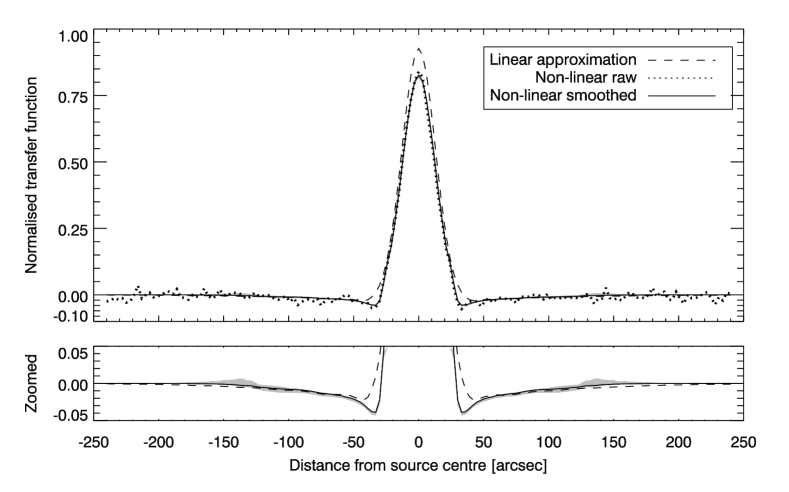
Figure 1: Comparison of the various techniques to estimate the PCA cleaning point source transfer function for a set of 43 observations of a single ASTE science field. See text for full discussion of interpretation. The grey shaded region indicates the envelope of 20 calculations of the non-linear smoothed kernel using different locations for the simulated sources.

Figure 2: (a) Comparison of transfer functions calculated using 3 simulated sources of varying brightness at fixed locations. (b) A zoomed portion of (a) showing that the primary impact of non-linearity is to make the negative sidelobes shallower as source brightness increases. (c) The change in measured flux (relative to peak) for $20\sigma$ and $5\sigma$ sources when they are optimally filtered using the the standard transfer function derived from $10\sigma$ sources. The peak flux and all other pixels are shifted by $<1.5\%$ of the peak flux and therefore the transfer function does not introduce significant systematic error for sources of typical detection significance.

The ultimate test of the revised transfer function is whether it succeeds in producing the correct flux when analyzing data with simulated sources reduced blindly. 23 simulated maps were produced in each of which were inserted 4 simulated sources at varying locations far from resolved sources with fluxes ranging from 3 to 20mJy. This spans a detection significance range of $\sim$$4-30\sigma$. The sources were placed at the centre of 3″ pixels in the portion of the map with sufficient and uniform coverage to be used for selecting true astrophysical sources. This simulation also tests for any impact that a moderate increase in source density may have upon the transfer function as 7 simulated sources will ultimately be inserted into the map (4 “test” sources whose flux we intend to measure and 3 sources whose sole purpose is to measure the transfer function). The maps were then optimally filtered using the revised transfer function estimate and the detected flux and estimated noise at the known source location was compared to the known input flux (Fig. 3). The input and observed fluxes are found to be consistent; there is a small negative offset that is consistent with the mean value (-0.24 mJy) of the pixels at the chosen input locations. Because the map has an overall mean of zero and we have chosen locations that are far from bright, positive sources of flux, it is reasonable to find a small, negative offset. The absence of systematic effects from source location (Fig. 1) or source flux density (Fig. 3) may be an indication that, although the transfer function must be varying as a function of time (the number of eigenfunctions removed from each chunk of data is not constant), it varies more slowly than the time taken to cover the useful coverage region of the maps. Thus the variations are captured equally well by any simulated source within this region.

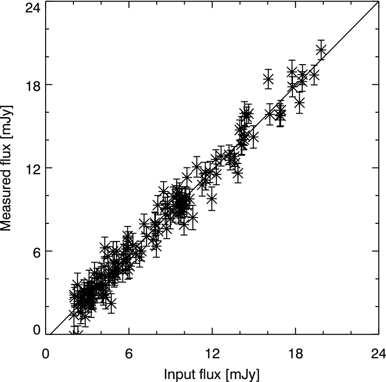
Figure 3: A comparison of the observed flux in optimally filtered maps at the locations where simulated sources of known flux have been inserted. The transfer function is consistent with unity and has a small, negative offset which can be explained by observing that the mean value of the chosen pixel locations was -0.24 mJy in the recorded map. The best-fit line, $y=-0.3\pm 0.2+(1.015\pm 0.018)x$, is shown in red.

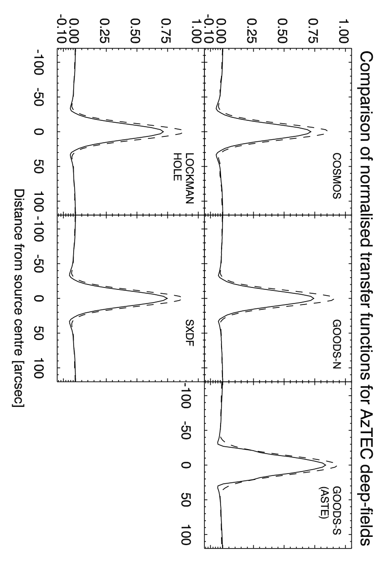
Figure 4: Comparison of the linear approximation (dashed) and simulated source (solid) techniques to estimate the PCA cleaning point source transfer function for previously published AzTEC catalogues. It is observed that the impact is greater for the 4 JCMT fields than for the ASTE field shown as well as in internal analysis for ASTE fields not yet published. This may be due to the greater atmospheric fluctuations at the JCMT site.

4 Revised catalogues

When this technique is applied to other fields (Fig. 4), we observe, for AzTEC data taken while installed at the ASTE, that the revised transfer function corrects both signal and noise by $\sim$+10 per cent, in each field. Similarly, we find a correction of +15-25 per cent in the fields observed while AzTEC was installed at the James Clerk Maxwell Telescope (JCMT). This is consistent with the notion that some of the point source signal is present in the largest eigenfunctions removed by PCA. The larger impact for the JCMT data may be taken as a sign that the non-linear nature of PCA is more greatly affected by the worse observing conditions at Mauna Kea as compared to the Atacama Desert in Chile. We wish to emphasize that, for each observation, simulating the signal of interest and directly observing the impact of PCA or another non-linear technique is a surer approach than building expectations based on prior results.

Several previous publications have released point source catalogues from the AzTEC instrument while it was installed at the JCMT and the ASTE. These catalogues are reproduced below using the revised photometry, along with deboosted fluxes calculated from a forthcoming number counts analysis to be presented in Scott, et al., submitted. The AzTEC deboosting algorithm (Austermann et al., 2009) accounts for the fact that, for a source population that declines steeply with flux, any given source is more likely to be a relatively plentiful dim source “boosted” upward by noise than a rare bright source on top of a negative noise fluctuation. The algorithm makes the assumption that the flux in a given pixel is emitted from a single source. This assumption may be invalid owing to source confusion from the finite AzTEC beam, however it has been shown to yield results consistent with a parametric frequentist “$P(d)$” approach (Perera et al., 2008) that attempts to account for confusion through comparison of the recorded map to simulations of noise and source populations convolved with the beam. The number counts analysis incorporates the revised photometry and is based upon measurements in all blank fields, including those below, surveyed by the AzTEC instrument. Because the effect of deboosting is a slowly changing function of the sky model prior assumed, the deboosted values given below are reasonable even if the inclusion of other fields introduces a potential bias to the sky model. The deboosted fluxes also include correction for a bias introduced by searching for a signal peak in the presence of noise. The number counts analyses previously presented will be affected by the change in photometry in 2 ways. First, the estimated counts at a given brightness value are now appropriate for a slightly increased source brightness. Second, an integral step in computing number counts is dividing by the estimated completeness for a given flux in the map. Because the estimated error is higher under the revised transfer function, any given flux value will be less complete; this effect will be more pronounced at moderate signal-to-noise ($\sim$3-5) where the completeness is rapidly dropping from unity toward zero.

The details of the analysis for each field do not differ appreciably from that previously performed, except for the change in photometry. We provide references to these analyses for the interested reader. We present the catalogues using the significance and spatial cuts applied by each catalogue’s respective author. In each case the expected false detection rate is estimated using the defined cuts and did not change greatly from that using the transfer function derived from the linear approximation. Source names and numeric identifiers for sources which were previously detected are retained; however a common format has been chosen: “AzTEC/field#”, where ‘#’ indicates order of discovery rather than strictly being based upon detection significance in these revised catalogues. Thus newly discovered sources with higher significance than a previously discovered source will appear at the end of these catalogs and a slight shuffling (in significance) of previously discovered sources will occur for the reasons discussed above.

4.1 COSMOS / JCMT

The COSMOS survey (Scott et al., 2008; Austermann et al., 2009) was undertaken by the AzTEC instrument in 2005 while it was installed at the JCMT. A revised catalogue is shown in Table 4.1. A spatial cut (0.15 deg²) was applied by taking only pixels within the map whose weighting (a combination of noise in the data and amount of time spent observing that pixel) are greater than 75 per cent of the map’s characteristic value (roughly the maximum). A significance cut is applied by taking only sources whose signal to noise ratio are greater than 3.5. We have conservatively over-estimated the false detection rate to be 25 per cent ($\sim$12 sources) using the number of sources “detected” in pure noise realisations of the field. This choice is conservative because faint sources contribute to flux in nearly every pixel in the map and therefore the likelihood of finding a source at any pixel is greater than it otherwise would be (Perera et al., 2008; Scott et al., 2010). The difference between this technique and one that attempts to account for this effect through simulations of source populations can be a factor of 2 or greater.

Table 1: The AzTEC point source catalogue for the COSMOS field as observed from the JCMT.

Source ID	Nickname	S/N	$S_{1.1\text{mm}}$	$S^{\text{corrected}}_{1.1\text{mm}}$	$P(<0)$	Flux	Noise	$\theta$
			[mJy]	[mJy]		increase	increase
AzTEC_J095942.68+022936.1	AzTEC/COSMOS.1	8.1	$12.4\pm 1.5$	$10.8\pm^{+1.5}_{-1.6}$	0.00	16.0%	18.9%	0.6″
AzTEC_J100008.03+022612.0	AzTEC/COSMOS.2	7.3	$11.3\pm 1.5$	$9.7\pm^{+1.4}_{-1.7}$	0.00	16.8%	18.8%	0.6″
AzTEC_J100018.26+024830.1	AzTEC/COSMOS.3	6.5	$10.7\pm 1.6$	$8.6\pm^{+1.7}_{-1.7}$	0.00	20.9%	18.8%	1.0″
AzTEC_J100006.40+023839.9	AzTEC/COSMOS.4	6.2	$9.0\pm 1.5$	$7.3\pm^{+1.5}_{-1.5}$	0.00	17.1%	18.8%	0.3″
AzTEC_J100019.73+023205.8	AzTEC/COSMOS.5	6.0	$9.1\pm 1.5$	$7.3\pm^{+1.6}_{-1.5}$	0.00	15.4%	18.8%	0.6″
AzTEC_J100020.72+023518.3	AzTEC/COSMOS.6	5.9	$8.8\pm 1.5$	$6.9\pm^{+1.6}_{-1.4}$	0.00	18.8%	18.8%	0.7″
AzTEC_J095959.33+023445.8	AzTEC/COSMOS.7	5.4	$8.0\pm 1.5$	$6.0\pm^{+1.7}_{-1.4}$	0.00	12.8%	18.8%	0.5″
AzTEC_J095957.22+022729.3	AzTEC/COSMOS.8	5.5	$8.4\pm 1.5$	$6.5\pm^{+1.6}_{-1.6}$	0.00	16.7%	18.8%	1.2″
AzTEC_J095931.82+023040.1	AzTEC/COSMOS.9	5.0	$7.5\pm 1.5$	$5.5\pm^{+1.6}_{-1.6}$	0.00	12.3%	18.7%	0.6″
AzTEC_J095930.76+024034.2	AzTEC/COSMOS.10	5.1	$7.3\pm 1.4$	$5.5\pm^{+1.4}_{-1.6}$	0.00	17.8%	18.7%	0.7″
AzTEC_J100008.79+024008.0	AzTEC/COSMOS.11	5.1	$7.3\pm 1.4$	$5.5\pm^{+1.5}_{-1.5}$	0.00	18.9%	18.8%	0.5″
AzTEC_J100035.37+024352.3	AzTEC/COSMOS.12	4.9	$7.5\pm 1.5$	$5.5\pm^{+1.5}_{-1.7}$	0.00	22.2%	18.7%	1.0″
AzTEC_J095937.05+023315.4	AzTEC/COSMOS.13	4.6	$6.9\pm 1.5$	$4.9\pm^{+1.5}_{-1.7}$	0.00	15.2%	18.8%	0.9″
AzTEC_J100010.00+023021.2	AzTEC/COSMOS.14	4.8	$7.3\pm 1.5$	$5.2\pm^{+1.6}_{-1.6}$	0.00	21.3%	18.8%	1.7″
AzTEC_J100013.22+023428.1	AzTEC/COSMOS.15	4.4	$6.5\pm 1.5$	$4.5\pm^{+1.5}_{-1.7}$	0.00	13.0%	18.7%	0.5″
AzTEC_J095950.29+024416.2	AzTEC/COSMOS.16	4.5	$6.3\pm 1.4$	$4.5\pm^{+1.4}_{-1.6}$	0.00	17.5%	18.7%	0.5″
AzTEC_J095939.29+023408.2	AzTEC/COSMOS.17	4.4	$6.5\pm 1.5$	$4.5\pm^{+1.5}_{-1.7}$	0.01	18.7%	18.8%	0.0″
AzTEC_J095943.05+023540.2	AzTEC/COSMOS.18	4.3	$6.3\pm 1.5$	$4.3\pm^{+1.6}_{-1.7}$	0.01	18.2%	18.8%	0.5″
AzTEC_J100028.93+023200.3	AzTEC/COSMOS.19	4.4	$6.6\pm 1.5$	$4.5\pm^{+1.6}_{-1.7}$	0.00	22.4%	18.8%	0.2″
AzTEC_J100020.16+024117.2	AzTEC/COSMOS.20	4.0	$5.8\pm 1.4$	$3.7\pm^{+1.6}_{-1.6}$	0.01	12.0%	18.6%	2.0″
AzTEC_J100002.73+024645.0	AzTEC/COSMOS.21	4.2	$5.9\pm 1.4$	$4.0\pm^{+1.5}_{-1.6}$	0.01	19.3%	18.9%	1.1″
AzTEC_J095950.78+022828.3	AzTEC/COSMOS.22	4.3	$6.6\pm 1.5$	$4.3\pm^{+1.7}_{-1.6}$	0.01	22.6%	18.9%	0.7″
AzTEC_J095931.58+023601.6	AzTEC/COSMOS.23	3.9	$5.7\pm 1.5$	$3.5\pm^{+1.6}_{-1.7}$	0.02	11.8%	18.8%	0.9″
AzTEC_J100038.83+023843.6	AzTEC/COSMOS.24	3.8	$5.6\pm 1.5$	$3.3\pm^{+1.7}_{-1.6}$	0.02	11.2%	18.7%	1.1″
AzTEC_J095950.39+024759.4	AzTEC/COSMOS.25	4.2	$6.0\pm 1.4$	$4.0\pm^{+1.5}_{-1.6}$	0.01	21.7%	19.0%	1.6″
AzTEC_J095959.58+023818.4	AzTEC/COSMOS.26	4.0	$5.9\pm 1.5$	$3.8\pm^{+1.5}_{-1.7}$	0.01	18.3%	18.8%	1.7″
AzTEC_J100039.11+024052.4	AzTEC/COSMOS.27	3.9	$5.8\pm 1.5$	$3.6\pm^{+1.6}_{-1.7}$	0.02	15.0%	18.7%	0.2″
AzTEC_J100004.54+023040.1	AzTEC/COSMOS.28	3.9	$6.0\pm 1.5$	$3.7\pm^{+1.7}_{-1.8}$	0.02	17.3%	18.8%	0.4″
AzTEC_J100026.69+023753.6	AzTEC/COSMOS.29	3.9	$5.8\pm 1.5$	$3.6\pm^{+1.6}_{-1.7}$	0.02	17.3%	18.8%	1.0″
AzTEC_J100003.87+023254.1	AzTEC/COSMOS.30	4.1	$6.1\pm 1.5$	$3.8\pm^{+1.7}_{-1.6}$	0.01	22.5%	18.7%	0.4″
AzTEC_J100034.60+023101.9	AzTEC/COSMOS.31	3.9	$5.9\pm 1.5$	$3.5\pm^{+1.7}_{-1.7}$	0.02	17.2%	18.7%	0.6″
AzTEC_J100020.66+022452.8	AzTEC/COSMOS.32	3.6	$6.1\pm 1.7$	$3.2\pm^{+1.7}_{-2.2}$	0.05	13.6%	18.8%	0.9″
AzTEC_J095911.70+023909.6	AzTEC/COSMOS.33	3.9	$6.0\pm 1.6$	$3.6\pm^{+1.7}_{-1.8}$	0.03	21.8%	19.0%	0.3″
AzTEC_J095946.66+023541.8	AzTEC/COSMOS.34	3.6	$5.3\pm 1.5$	$2.9\pm^{+1.6}_{-1.8}$	0.04	13.5%	18.8%	0.8″
AzTEC_J100026.69+023128.1	AzTEC/COSMOS.35	3.8	$5.8\pm 1.5$	$3.5\pm^{+1.6}_{-1.8}$	0.03	21.4%	18.8%	0.4″
AzTEC_J095914.01+023424.0	AzTEC/COSMOS.36	3.7	$5.6\pm 1.5$	$3.3\pm^{+1.6}_{-1.8}$	0.03	19.0%	18.8%	1.1″
AzTEC_J100016.31+024716.0	AzTEC/COSMOS.37	3.5	$5.3\pm 1.5$	$2.8\pm^{+1.7}_{-1.7}$	0.05	14.7%	18.7%	0.6″
AzTEC_J095951.72+024338.0	AzTEC/COSMOS.38	3.6	$5.1\pm 1.4$	$2.8\pm^{+1.6}_{-1.6}$	0.04	15.2%	18.7%	0.8″
AzTEC_J095958.28+023608.2	AzTEC/COSMOS.39	3.6	$5.3\pm 1.5$	$2.8\pm^{+1.7}_{-1.7}$	0.04	16.3%	18.7%	0.4″
AzTEC_J100031.09+022749.9	AzTEC/COSMOS.40a	3.3	$5.4\pm 1.6$	–	–	10.7%	18.9%	–
AzTEC_J095957.33+024139.9	AzTEC/COSMOS.41a	3.4	$4.9\pm 1.4$	–	–	13.4%	18.8%	–
AzTEC_J095930.37+023437.9	AzTEC/COSMOS.42	3.5	$5.2\pm 1.5$	$2.8\pm^{+1.6}_{-1.9}$	0.05	15.1%	18.8%	1.1″
AzTEC_J100023.90+022950.2	AzTEC/COSMOS.43	3.5	$5.4\pm 1.5$	$2.8\pm^{+1.7}_{-1.8}$	0.05	16.3%	18.7%	0.8″
AzTEC_J095920.62+023417.9	AzTEC/COSMOS.44a	3.3	$5.0\pm 1.5$	–	–	10.6%	18.8%	–
AzTEC_J095932.26+023648.3	AzTEC/COSMOS.45	3.8	$5.5\pm 1.5$	$3.3\pm^{+1.6}_{-1.7}$	0.03	24.8%	18.7%	0.7″
AzTEC_J100000.79+022635.9	AzTEC/COSMOS.46	3.6	$5.6\pm 1.5$	$3.0\pm^{+1.7}_{-1.9}$	0.04	19.9%	18.8%	0.3″
AzTEC_J095938.54+023146.4	AzTEC/COSMOS.47	3.5	$5.3\pm 1.5$	$2.8\pm^{+1.7}_{-1.8}$	0.05	17.6%	18.8%	0.7″
AzTEC_J095943.85+023329.9	AzTEC/COSMOS.48a	3.3	$5.0\pm 1.5$	–	–	12.4%	18.7%	–
AzTEC_J100039.05+024129.8	AzTEC/COSMOS.49	3.7	$5.5\pm 1.5$	$3.2\pm^{+1.6}_{-1.9}$	0.04	23.7%	18.8%	0.7″
AzTEC_J100012.41+022657.6	AzTEC/COSMOS.50	3.6	$5.6\pm 1.5$	$3.2\pm^{+1.6}_{-2.0}$	0.04	23.4%	18.8%	0.7″

The columns are as follows: (1) AzTEC source name, including RA and declination based on centroid position; (2) nickname;      (3) signal-to-noise of the detection; (4) measured $1100\mu$m flux density and error; (5) flux density and 68 per cent confidence      interval of the deboosted flux density, including corrections for the bias to peak locations in the map; (6) probability that the      source will deboost to $S<0$ assuming the number counts prior based on all AzTEC measurements; (7,8) the relative increase      in flux and noise estimate for each source if it was detected in the previously release catalogue; (9) change in location of the      centroided source position if it was detected in both catalogs. (^a) indicates a source passed a significance test in the original      catalog, but not the same test in the new catalog. (^b) indicates a source passed a significance test in the new catalog, but not      the same test in the original catalog. In each case, an estimate for the missing quantity is made from the nearest pixel in the      map in which the test did not succeed.

4.2 GOODS North / JCMT

The GOODS North field is commonly observed at many wavelengths. A revision of the catalogue presented in Perera et al. (2008) is shown in Table 4.2. Similar cuts are taken at the 70 per cent coverage region (0.07 deg²) and detection significances above 3.5. The false detection rate was estimated using pure noise maps to be 13 per cent ($\sim$4-5 sources).

Table 2: The AzTEC point source catalogue for the GOODS North field.

4.3 Lockman Hole / JCMT

The Lockman Hole survey (Austermann et al., 2010) was undertaken by the AzTEC instrument in 2005 while it was installed at the JCMT and formed part of the 1.1mm follow-up to the SCUBA/SHADES project. A revised catalogue is shown in Table 4.4. The 50 per cent coverage region (0.31 deg²) was selected as a spatial cut, but a different significance cut was used. Deboosting can also be used as a proxy for whether a source is likely to be real. If the likelihood of deboosting to 0 flux is significant, then that source can be excluded from the catalogue. Only sources with less than 10 per cent likelihood of deboosting to 0 flux are taken. The false detection rate using these cuts was estimated by the technique described in Perera et al. (2008); Scott et al. (2010). In this technique, false detection rates are estimated by fully simulating maps using noise estimates and a signal estimate using the number counts used in deboosting measured fluxes. Using this technique, the false detection rate was estimated to be 20 per cent ($\sim$20 sources).

Table 3: The AzTEC point source catalogue for the Lockman Hole field.

Table 4: continued

4.4 Subaru XMM-Newton Deep Field / JCMT

The Subaru XMM-Newton Deep Field (SXDF) was also surveyed as part of the SHADES followup project. A revised catalogue is shown in Table 4.4. The same cuts as in the Lockman Hole field are applied with a resulting survey area of 0.37 deg². Using the simulated map technique, the false detection rate was estimated to be 25 per cent ($\sim$16 sources). The near doubling of the number of detected sources under the revised kernel is an artefact of using the deboosted flux values and a different number counts model as a catalogue cut in a population of sources whose numbers grow rapidly with declining flux.

Table 5: The AzTEC point source catalogue for the Subaru XMM-Newton Deep Field.

Table 6: continued

4.5 GOODS South / ASTE

The GOODS South field is another commonly observed field and among the first chosen for AzTEC when it was moved from the JCMT to the ASTE in 2007. A revision of the confusion-limited catalogue presented in Scott et al. (2010) is shown in Table LABEL:tbl:goodss. Sources of significance greater than 3.5 in the 50 per cent coverage region (0.08 deg²) are presented. Using the same false detection estimate technique as was used for the COSMOS field, we estimate a false detection rate of 6 per cent ($\sim$3 sources). Many of the sources appear to be somewhat extended, a sign of the highly confused nature of the map. Notably, we present the 2nd most significant detection under the assumptions that the flux is the result of a single source or, alternatively, from two nearby sources. Other sources at modest signal-to-noise do not provide sufficient constraints to multiple source models. 8 new sources are found in the revised catalogue, many from regions of the map which appear extended.

Table 7: The AzTEC point source catalogue for the GOODS South field.

4.6 Observations

The detection significance of any given source may change owing to the greater accuracy of flux and noise estimation using the revised photometry technique. Nonetheless, viewing the catalogues as a whole, detection significance is seen not to be greatly impacted because the photometry affects both signal and noise. Likewise, the false detection rates in the fields were unchanged. The vast majority of sources that passed a significance test in a prior catalogue pass it again in the revised catalogue. In fact, the increased number of sources in the majority of the revised catalogues suggest a slight systematic upward shift in detection significance; the exponentially increasing number of dim sources in these fields allow a slight shift to increase considerably the number of detected sources.

5 Future Work

The reviewer suggested a potentially simpler technique for estimating the transfer function that would not require the noise mitigating steps described. Rather than calculating the transfer function by differencing a source-added map from the recorded map, one would calculate the eigenvectors from the source-added timestreams and remove them from source-only timestreams. The eigenfunctions identified by PCA cleaning would have the proper impact of sources included, but the transfer function estimated would not include the small difference in noise realisations between the two maps. This should produce a result identical to the analysis shown in a much simpler fashion. This manuscript documents the technique used in several AzTEC publications in 2011-2012 (Humphrey et al., 2011; Yun et al., 2011; Aretxaga et al., 2011; Kim et al., 2012). If the technique is revised further to include this suggestion or others, it will be documented in subsequent publications.

6 Conclusions

A general approach to estimating the transfer function of non-linear techniques has been described and applied to the specific case of principal component analysis (PCA). Simulations support the accuracy of the results and that PCA has a transfer function which is effectively linear for point sources of typical detection significance. The resulting transfer function has been used to correct the catalogue values for the flux, location and significance of point sources in existing AzTEC maps. Mean source detection significance is not strongly impacted by the photometry correction and may be slightly enhanced.

7 Acknowledgments

This work has been made possible by generous support from the Kavli Foundation and the Gordon and Betty Moore Foundation. Additional support for this analysis has been provided in part by National Science Foundation grants 0540852, 0838222 and 0907952. KSS is supported by the National Radio Astronomy Observatory, which is a facility of the National Science Foundation operated under cooperative agreement by Associated Universities, Inc. We would like to acknowledge the assistance of Jack Sayers and Stephan Meyer for useful comments on the analysis presented herein. We also thank the observatory staff of the JCMT and ASTE who made these observations possible.

References

- Anton (1994) Anton H., 1994, Elementary Linear Algebra, 7th edn. Wiley, New York
- Aretxaga et al. (2011) Aretxaga I., et al., 2011, MNRAS, 415, 3831
- Austermann et al. (2009) Austermann J. E., et al., 2009, MNRAS, 393, 1573
- Austermann et al. (2010) Austermann J. E., et al., 2010, MNRAS, 401, 160
- Enoch et al. (2006) Enoch M. L., et al., 2006, ApJ, 638, 293
- Humphrey et al. (2011) Humphrey A., et al., 2011, MNRAS, 418, 74
- Kim et al. (2012) Kim M. J., et al., 2012, ApJ, 746, 11
- Kovács (2008) Kovács A., 2008, in Society of Photo-Optical Instrumentation Engineers (SPIE) Conference Series Vol. 7020 of Presented at the Society of Photo-Optical Instrumentation Engineers (SPIE) Conference, CRUSH: fast and scalable data reduction for imaging arrays
- Lay & Halverson (2000) Lay O. P., Halverson N. W., 2000, ApJ, 543, 787
- Perera et al. (2008) Perera T. A., et al., 2008, MNRAS, 391, 1227
- Sayers (2007) Sayers J., 2007, PhD thesis, California Institute of Technology
- Sayers et al. (2010) Sayers J., et al., 2010, ApJ, 708, 1674
- Scott et al. (2008) Scott K. S., et al., 2008, MNRAS, 385, 2225
- Scott et al. (2010) Scott K. S., et al., 2010, MNRAS, 405, 2260
- Wilson et al. (2008) Wilson G. W., et al., 2008, MNRAS, 386, 807
- Yun et al. (2011) Yun M. S., et al., 2011, MNRAS, p. 2141