Radiation Transfer of Models of Massive Star Formation. I. Dependence on Basic Core Properties

Abstract

Radiative transfer calculations of massive star formation are presented. These are based on the Turbulent Core Model of McKee & Tan and self-consistently included a hydrostatic core, an inside-out expansion wave, a zone of free-falling rotating collapse, wide-angle dust-free outflow cavities, an active accretion disk, and a massive protostar. For the first time for such models, an optically thick inner gas disk extends inside the dust destruction front. This is important to conserve the accretion energy naturally and for its shielding effect on the outer region of the disk and envelope. The simulation of radiation transfer is performed with the Monte Carlo code of Whitney, yielding spectral energy distributions (SEDs) for the model series, from the simplest spherical model to the fiducial one, with the above components each added step-by-step. Images are also presented in different wavebands of various telescope cameras, including Spitzer IRAC and MIPS, SOFIA FORCAST and Herschel PACS and SPIRE. The existence of the optically thick inner disk produces higher optical wavelength fluxes but reduces near- and mid-IR emission. The presence of outflow cavities, the inclination angle to the line of sight, and the thickness of the disk all affect the SEDs and images significantly. For the high mass surface density cores considered here, the mid-IR emission can be dominated by the outflow cavity walls, as has been suggested by De Buizer. The effect of varying the pressure of the environment bounding the surface of the massive core is also studied. With lower surface pressures, the core is larger, has lower extinction and accretion rates, and the observed mid-IR flux from the disk can then be relatively high even though the accretion luminosity is lower. In this case the silicate absorption feature becomes prominent, in contrast to higher density cores forming under higher pressures.

1. Introduction

“How do massive stars form?” is still a debated question (e.g., Beuther et al. 2007). One basic problem is massive protostars become so luminous that radiation pressure may stop the accretion and growth of the star. One possible mechanism to form a massive star can be considered as a scaled-up version of low-mass star formation. If the gas is turbulent and threaded by sufficiently strong magnetic fields then fragmentation may be suppressed for cores much more massive than the Jeans mass. The conditions leading to this suppression should be relatively rare since massive stars are rare and make up only a small mass fraction of the final star cluster. These massive cores are expected to form from highly pressurized clumps of gas, in which case they start with high densities, short free-fall times and therefore high accretion rates. This is the basic scenario of the Turbulent Core Model (McKee & Tan 2003, hereafter MT03). Other radically different possibilities are that massive stars form through stellar mergers (Bonnel et al. 1998) or accrete most of their mass from initially unbound material (competitive accretion model, Bonnel et al. 2001, Bonnel et al. 2004, Bate 2009a, b).

Answering this question is difficult observationally because massive star formation occurs in distant and highly obscured regions. However, with the improving sensitivity and spatial resolution provided by the instruments such as the Herschel Space Telescope, Stratospheric Observatory for Infrared Astronomy (SOFIA), Gran Telescopio Canarias (GTC) - CanariCam, the James Webb Space Telescope and Thirty-Meter class telescopes, we expect to see a faster advance in the research of massive star formation and hope this question can be finally solved.

In order to interpret observations such as spectral energy distributions (SEDs) or images, and then have a better understanding of the properties of a massive protostar and its evolution, a number of models have already been developed to fit or compare with observations. For example, Robitaille et al. (2006) have developed a very impressive model grid containing 200,000 SEDs covering a large parameter space, which is publicly available and now widely used (referred to below as the “Robitaille model”). However, this grid mainly covers low-mass young stellar objects (YSOs) and when massive protostars are considered, they do not have the properties expected for fiducial parameters of the turbulent core model. Also these models do not consider the presence of an optically thick gaseous disk inside the dust destruction front. Molinari et al. (2008) used the same methods employed by the Robitaille model but now for protostellar parameters based on the turbulent core model, to developed a SED model grid for massive YSOs. They found that the SED can be a diagnostic tool to determine the evolutionary stage of a massive YSO. However, in this work the representation of the turbulent core model is quite approximate and limitations of the Robitaille model framework are still present. Chakrabarti & McKee (2005) developed an analytic solution for far-IR SED of a protostar embedded in a spherically symmetric molecular cloud, but this method could not allow for presence of accretion disks and protostellar outflow cavities. Indebetouw et al. (2006) investigated the effects of clumpy structures in the molecular envelope around massive protostars. However, again, their models were not tuned to the parameters of the turbulent core model: for example, they considered much more massive structures (e.g. $\sim 5\times 10^{4}\;M_{\odot}$ contained in a sphere of radius 2.5 pc), more representative of star forming clumps that form entire star clusters. They did not consider protostellar disks.

Our aim is thus to develop a new model of massive protostars, based on the Turbulent Core Model of McKee & Tan (2002) and MT03, including all the important components self-consistently, and then perform simulations of the radiation transfer to see whether different components or evolutionary stages are represented in the SEDs and images. Starting with a fiducial hydrostatic core of $60\;M_{\odot}$ bounded by the pressure of a self-gravitating clump of mean mass surface density $\Sigma_{\rm cl}=1\>{\rm g\>cm^{-2}}$, we then consider its appearance once an $8\;M_{\odot}$ protostar has formed at its center. We develop a series of protostellar models of increasing realism: starting with a simple hydrostatic core, we then apply the inside-out expansion wave solution (Shu 1977), but generalized to singular polytropic spheres (McLaughlin & Pudritz 1997) and the free-fall rotating collapse solution by Ulrich (1976). A circumstellar disk is expected to form around the protostar and this is important to transfer angular momentum and to solve the radiation pressure problem (e.g. Jijina & Adams 1996, Krumholz et al. 2007). Presently, there is evidence for rotating toroids around massive protostars (e.g. Beltrán et al. 2005) but little direct evidence for Keplerian protostellar disks, which will probably require the angular resolution of ALMA. We include the disk with an $\alpha$-disk model (Shakura & Sunyaev 1973). Unlike Robitaille et al. (2006) and Molinari et al. (2008), we include an optically thick inner disk with gas opacities inside the dust destruction radius, which is important to conserve the accretion energy naturally. Accretion is expected to drive strong bipolar outflows and sweep up the material in the core and form cavities. These outflow cavities have been observed around massive protostars and may determine the mid-IR morphology (e.g., De Buizer 2006).

The assumptions of each component of our model and the model series are introduced in detail in the next section. In Section. 3, we discuss our simulations, including the Monte Carlo radiation transfer code, and the dust and gas opacities we use. In Section. 4, we present the SED and image results of our models. In Section. 5, we summarize our main results, including a comparison of our model with other works. In future papers we will examine additional refinements, especially the development and material content of the outflow cavities, and present results of the evolutionary sequence of massive star formation based on the fiducial model we have started to develop here.

2. Massive Protostar Model

2.1. Envelope

2.1.1 Hydrostatic Outer Envelope

Following MT03 and Tan (2008), we define a “star-forming core” as a region of a molecular cloud that will form a single star or close binary, and assume it is self-similar, self-gravitating in near virial equilibrium and spherical. The density and pressure each have power-law dependencies on radius, $\rho\propto r^{-k_{\rho}}$ and $P\propto r^{-k_{p}}$. This smooth power-law density distribution is only an approximation, especially given that massive cores in virial equilibrium but with gas temperatures $\sim 10\;{\rm K}$ must be supported by non-thermal forms of pressure support, such as turbulence and/or magnetic fields. Clumpy substructures are likely to form inside a turbulent core and this will affect radiative transfer through the core - basically making it somewhat easier for shorter wavelength photons to propagate through the core. Indebetouw et al. (2006) performed radiative transfer models of clumpy cores. However, given the uncertain nature of the clumping, we defer such considerations to a future paper, and first calculate the properties of smoothly distributed gas and dust.

From the above power law distributions, it follows that the core is polytropic with $P\propto\rho^{\gamma_{p}}$. The case with $\gamma_{p}=1$ is a singular isothermal sphere (Shu 1977) and in the other limit $\gamma_{p}=0$ corresponds to a logotropic sphere (McLaughlin & Pudritz 1996, 1997). For the models presented here, we follow MT03 and adopt $k_{\rho}=1.5$, thus $\gamma_{p}=\frac{2}{3}$ and $k_{p}=1$. The equation of hydrostatic equilibrium gives

$$M(r)=\frac{k_{p}c^{2}r}{G},$$ (1)

and

$$\rho(r)=\frac{(3-k_{\rho})(k_{\rho}-1)c^{2}}{2\pi Gr^{2}},$$ (2)

where $c=(P/\rho)^{1/2}$ is the effective sound speed.

We assume the total mass in the core is 60 $M_{\odot}$. If the efficiency $\epsilon_{*f}$ is 0.5, which is estimated from low-mass cases (Matzner & McKee 2000), a star with mass $m_{*f}=\epsilon_{*f}M_{\mathrm{core}}=30\;M_{\odot}$ can finally form out of the core. For a core with such mass, the core radius is (eq. (20) in MT03)

$$R_{\mathrm{core}}=0.057\Big{(}\frac{M_{\mathrm{core}}}{60\;M_{\odot}}\Big{)}^{1/2}\Sigma_{\mathrm{cl}}^{-1/2}\;\mathrm{pc},$$ (3)

where $\Sigma_{\mathrm{cl}}$ is the mean surface density in the molecular clump in which the core is embedded, and $1\;\mathrm{g/cm}^{-2}$ is used as a fiducial value. We also consider models with higher and lower values of $\Sigma_{\rm cl}$.

2.1.2 Expansion Wave

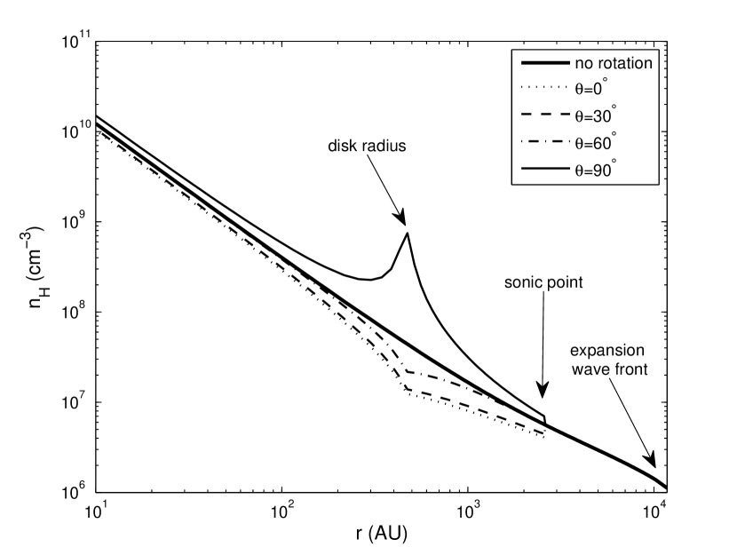
Figure 1.— Density distribution with radius $r$ (left panel) and polar angle $\theta$ (right panel). $n_{\mathrm{He}}=0.1n_{\mathrm{H}}$ is assumed here. In the left panel, different curves correspond to different polar angles, which is $0^{\circ}$ when along the rotation axis. The thick black curve is without any rotation effect for comparison. The right panel shows the density dependence on $\theta$ at $r=2r_{d}$ and $r=4r_{d}$.

Shu (1977) developed the inside-out expansion-wave solution for the problem of the gravitational collapse of an isothermal sphere. McLaughlin & Pudritz (1997) applied this solution to the collapse of a logotropic sphere and also gave the general formulae for a polytropic sphere. Following their work, we calculate the density profile in the core. A core with initial density profile of eq. (2) is not stable and a perturbation at the center can trigger collapse of the innermost region. The position where the material begins to fall progresses outward, which is called the expansion wave. While the material collapses inside the expansion wave front, the region outside it is still hydrostatic. The similarity is always kept during the whole collapse in this solution.

McLaughlin & Pudritz (1997) did not include the effect of magnetic fields which can help to support more mass in the core and increase the accretion rate after collapse starts. We estimate the effect of magnetic fields from the work of Li & Shu (1997), who found that the equilibrium surface density is increased by a factor of $(1+H_{0})$ when magnetic fields are considered, where $H_{0}$ is a parameter. So the real mass and density profile should increased by the same factor,

$$M(r,t)=M_{\mathrm{non}}(r,t)(1+H_{0})=m(x)(1+H_{0})a_{t}^{3}t/G,$$ (4)

and

$$\rho(r,t)=\rho_{\mathrm{non}}(r,t)(1+H_{0})=\frac{\alpha(x)(1+H_{0})}{4\pi Gt^{2}},$$ (5)

where $m(x)$ and $\alpha(x)$ are the similarity variables for mass and density, and $a_{t}=[K\gamma_{p}(4\pi Gt^{2})^{1-\gamma_{p}}]^{1/2}$ has dimension of velocity. In our case, $H_{0}$ is set to 1 following the assumption by MT03.

The collapsed mass at the center now is

$$M(0)=m(0)(1+H_{0})a_{t}^{3}t/G,$$ (6)

therefore,

$$M(0)\propto a_{t}^{3}t\propto t^{4-3\gamma_{p}},$$ (7)

and

$$\dot{M}(0)\propto t^{3-3\gamma_{p}}\propto t$$ (8)

in our case, which is consistent with the analysis of MT03. So, given a certain collapsed mass $M(0,t)$, with the star formation time (the time that the whole core takes to collapse, eq. (44) in MT03)

$$t_{*f}=1.29\times 10^{5}\Big{(}\frac{M_{\mathrm{core}}}{60\;M_{\odot}}\Big{)}^{1/4}\Sigma_{\mathrm{cl}}^{-3/4}\;\mathrm{yr}$$ (9)

and the final collapsed mass $M(0,t=t_{*f})=M_{\mathrm{core}}=60\;M_{\odot}$ (The whole core collapses at the end, either into the star-disk system or into the outflow and escapes), we can calculate $t$ and further the density $\rho(r,t)$, velocity $u(r,t)$ and mass $M(r,t)$ at that moment. At some time the expansion wave will reach the boundary of the core and lead to a backward wave, thus, for simplicity we choose such a collapsed mass that the expansion wave has not reached the core boundary yet. (We will discuss this in detail in Section 2.4.)

2.1.3 Rotating Infall

We consider a slowly rotating core. For simplicity, we only include the effect of rotation inside the sonic point, where the infall becomes supersonic. Once such infall starts, we expect it is difficult to transfer angular momentum from inside the sonic point to outside (Tan & McKee 2004). So we assume that the angular momentum is conserved inside the sonic point until gas accretes onto the star or disk.

We use the solution of Ulrich (1976) (referred to below as the “Ulrich solution”) to describe the velocity field and density profile inside the sonic point. This solution assumes that a particle with an initial distance $r_{\infty}$ from the center, an initial polar angle $\theta_{0}$ and angular velocity $\Omega_{\infty}$ about the axis of rotation, due to a point mass $M$ at the center, moves in a parabolic path described by

$$r=\frac{r_{d}\cos\theta_{0}\sin^{2}\theta_{0}}{\cos\theta_{0}-\cos\theta},$$ (10)

where

$$r_{d}=\frac{\Omega_{\infty}^{2}r_{\infty}^{4}}{GM}=\frac{j_{\infty}^{2}}{GM}.$$ (11)

All particles starting from a spherical shell of radius $r_{\infty}$ will hit the equatorial plane at radius $r<r_{d}$, so naturally $r_{d}$ can be thought of as the radius of the accretion disk.

$r_{d}$ is also the centrifugal radius which marks the radial extent of centrifugal balance, inside which the flow will become disk-like (e.g. Jijina & Adams 1996). It can be estimated as below:

$$r_{d}=\frac{6a_{g}}{5a_{i}}\beta r=\frac{6a_{g}}{5a_{i}}\beta\Big{(}\frac{M}{M_{\mathrm{core}}}\Big{)}^{\frac{1}{3-k_{\rho}}},$$ (12)

where $a_{g}=5|E_{\mathrm{grav}}|r/(3GM^{2})=(5/3)(3-k_{\rho})/(5-2k_{\rho})\rightarrow 1.25$, $a_{i}=2E_{\mathrm{rot}}/(Mr^{2}\Omega^{2})=(2/3)(3-k_{\rho})/(5-k_{\rho})\rightarrow 0.286$, and $\beta=E_{\mathrm{rot}}/|E_{\mathrm{grav}}|$ is set to have a fiducial value of 0.02 for the slowly rotating core, based on observations of low-mass cores (Goodman et al. 1993). For any spherical shell at radius $r$ inside the sonic point, it infalls following eq. (10), with $r_{d}$ to be the outer radius of the disk determined by the position of the sonic point.

$$r_{d}=\frac{6a_{g}}{5a_{i}}\beta\Big{(}\frac{M_{\mathrm{sp}}}{M_{\mathrm{core}}}\Big{)}^{\frac{1}{3-k_{\rho}}},$$ (13)

where $M_{\mathrm{sp}}$ is the mass inside the sonic point. In our fiducial case, when the collapsed mass is 10.67 $M_{\odot}$ (8 $M_{\odot}$ star and 2.67 $M_{\odot}$ disk, discussed in Section 2.5), the disk radius is 449 AU.

The rotation changes the density distribution from spherical symmetry to axissymmetry as below

$$\rho(r,\theta)\,\propto\,\Big{(}1+\frac{\cos\theta}{\cos\theta_{0}}\Big{)}^{-1/2}\Big{(}\frac{\cos\theta}{2\cos\theta_{0}}+\frac{r_{d}}{r}\cos^{2}\theta_{0}\Big{)}^{-1}.$$ (14)

This result is valid for an infall rate that is constant with radius, which is not exactly right for the expansion wave solution of a polytropic sphere. Thus we only scale the density distribution with the angular dependence of eq. (14) and keep the total mass in each shell unchanged, so that the infall rate is the same as the non-rotating case. Fig. 1 shows the radial density profiles at different polar angles (upper panel) and the density profiles with polar angle at different radii (lower panel), for a core with 10.67 $M_{\odot}$ collapsed at the center. In the upper panel, the thick black line shows the density profile in a non-rotating core. The thin curves correspond to different polar angles. There is a discontinuity at $r\sim 2500$ AU, which marks the position of the sonic point, only inside of which we consider rotation. For a real core, this discontinuity would not exist. The peaks and dips mark the disk radius $r_{d}$. The lower panel of Fig. 1 shows the dependence of density on $\theta$ at $2r_{d}$ and $4r_{d}$.

2.2. Accretion Disk

Inside the centrifugal radius $r_{d}$, the infalling flow is circularized and forms an accretion disk around the protostar. The disk can provide an efficient way to transfer angular momentum outwards and enable high accretion rates to form a massive star. The high accretion rate indicates that the disk is relatively massive (comparable to the star). But gravitational instability can become very efficient when the mass of the disk is high enough and lead it to fragment. We assume the disk mass is always a constant fraction of the stellar mass (Tan & McKee 2004):

$$m_{*d}=m_{*}+m_{d}=(1+f_{d})m_{*},$$ (15)

where $f_{d}$ is assumed to have a fiducial value of 1/3. Recently, Kratter et al. (2010) performed a numerical parameter study on accretion disks of massive stellar systems and found that a disk can be stable and does not fragment with an even higher disk-to-star mass ratio ($f_{d}\sim 1$).

We follow the description for the disk structure by Whitney et al. (2003b), which is a standard $\alpha$-disk (Shakura & Sunyaev 1973, Lynden-Bell & Pringle 1974, Pringle 1981, Bjorkman 1997, Hartmann et al. 1998) with density distribution

$$\rho=\rho_{0}\Big{(}1-\sqrt{\frac{r_{*}}{r}}\Big{)}\Big{(}\frac{r_{*}}{r}\Big{)}^{\alpha}\exp\Big{\{}-\frac{1}{2}\Big{(}\frac{z}{H(r)}\Big{)}^{2}\Big{\}},$$ (16)

where $r$ is the radial coordinate in the disk midplane, $z$ is the distance from the midplane, and $r_{*}$ is the stellar radius. Basically the density has a power-law profile with radius (smoothed at the innermost region) and a Gaussian profile with the height. $H$ is the scale height of the disk,

$$H=H_{0}\Big{(}\frac{r}{r_{*}}\Big{)}^{\beta}.$$ (17)

Thus, the disk structure is specified by following parameters: disk mass $m_{d}$, disk inner radius $r_{d,\mathrm{in}}$, disk outer radius $r_{d}$ (the centrifugal radius), disk scale height $H_{0}$ at the stellar surface, and the power indices $\alpha$ and $\beta$.

If the dust is the only source of opacity in the disk, then it equals to a disk truncated at dust destruction radius $r_{\mathrm{sub}}$, inside of which the temperature is too high for dust to exist. However, in reality, the gas opacity at the innermost region of the disk can be significant, so the disk should be optically thick down to the surface of the protostar. Thus, in our fiducial model, the inner radius of the disk is set to be the stellar radius.

We consider both geometrically thin ($H_{0}/r_{*}=0.01$) and moderately thick ($H_{0}/r_{*}=0.1$) disks to see the effects of the disk scale height. $H_{0}/r_{*}=0.01$ is the value used by (Whitney et al., 2003a, b). $H_{0}/r_{*}=0.1$ is closer to the aspect ratio expected for a disk composed of dust only and is a typical value for a moderately thick disk. For these cases, $\alpha$ and $\beta$ are chosen to be 1.875 and 1.125, respectively, as in the standard $\alpha$ disk models considered by Whitney. However, in our final fiducial model, we calculate the disk scale height, $\alpha$ and $\beta$ self-consistently from the gas and dust opacities, in which case, fitting with eq. (16) and (17) gives $H_{0}/r_{*}=0.06$ and $\alpha=1.75$, $\beta=1.08$.

In the limit of a slowly rotating protostar, the accretion luminosity from the system is

$$L_{\mathrm{acc}}=\frac{Gm_{*}\dot{m}}{r_{*}},$$ (18)

half of which is emitted from the viscous disk (disk accretion luminosity $L_{\mathrm{disk}}$) and the other half is emitted when the material hits the surface of the protostar (hot-spot luminosity $L_{\mathrm{hotspot}}$),

$$L_{\mathrm{disk}}=L_{\mathrm{hotspot}}=\frac{1}{2}L_{\mathrm{acc}}.$$ (19)

For simplicity, we add the hot-spot luminosity to the star’s homogeneously. The star then has a single, enhanced temperature to describe its black body spectrum. If the disk is truncated at $r_{d,\mathrm{in}}$, the disk luminosity will be

$$L_{\mathrm{disk}}(r_{d,\mathrm{in}})=\frac{Gm_{*}\dot{m}}{2r_{d,\mathrm{in}}}\Big{(}3-2\left(r_{*}/r_{d,\mathrm{in}}\right)^{1/2}\Big{)},$$ (20)

which indicates that only when the disk extends to the stellar radius can the total energy be conserved. In fact, the disk accretion luminosity is very sensitive to the inner radius of the disk. The accretion rate $\dot{m}$ of a massive protostar can be very high, reaching $\sim 10^{-4}-10^{-3}\;M_{\odot}$/yr. Here we adopt the protostar evolution model by MT03, which gives an accretion rate of $2.40\times 10^{-4}\;M_{\odot}$/yr for an 8 $M_{\odot}$ protostar in a 60 $M_{\odot}$ core. This accretion rate gives a disk luminosity and a hotspot luminosity which are comparable to the stellar luminosity.

The disk accretion rate is related to the $\alpha$ parameter of the disk by

$$\dot{m}=\sqrt{18\pi^{3}}\alpha_{\mathrm{disk}}V_{c}\rho_{0}H_{0}^{3}/r_{*}$$ (21)

with $V_{c}=(Gm_{*}/r_{*})^{1/2}$. Parameters used in our fiducial model correspond to a case with $\alpha_{\mathrm{disk}}=1.43$, which is consistent with the results of numerical simulations by Krumholz et al. (2007), in which they found an effective $\alpha_{\mathrm{disk}}\;\sim 1.0-1.6$.

Also, part of the energy may be used to drive the outflow (mechanical luminosity $L_{w}$, MT03). But for now we only consider the radiative luminosity from the disk and the hot-spot.

2.3. Outflow Cavity

Powerful bipolar outflows are ubiquitous phenomena around protostars (e.g. Königl & Pudritz 2000). The prevalent interpretation is that outflows are powered by accretion activity, being driven by spinning magnetic fields that thread the disk. There are several theoretical models to describe this process such as the X-wind from the innermost region of the disk (Shu et al. 1994) and disk wind model (Königl & Pudritz 2000).

A common feature of these models is the production of a bipolar outflow with momentum distribution $p_{w}\propto(\sin\theta_{w})^{-2}$ for $\theta_{w}>\theta_{w0}$, where $\theta_{w}$ is measured from the outflow axis and $\theta_{w0}\sim 10^{-2}$ is a small angle (Matzner & McKee 1999). On scales large compared to the source,

$$\frac{\mathrm{d}\dot{p}_{w}}{\mathrm{d}\Omega}=\frac{\dot{p}_{w}}{4\pi\ln(2/\theta_{w0})(1+\theta_{w0}^{2}-\cos^{2}\theta_{w})}.$$ (22)

We follow the discussion of Tan & McKee (2002). Assuming an opening angle of $\theta_{w,\mathrm{esc}}$ for the outflow cavity, the outflow material with $\theta_{w}>\theta_{w,\mathrm{esc}}$ cannot escape from the core and will go back to the infalling flow. We parameterize the fraction of the outflow momentum that escapes from the core with $f_{w,\mathrm{esc}}$. Najita & Shu (1994) showed that the velocity of the wind is approximately independent of the polar angle so that $f_{w,\mathrm{esc}}$ can also describe the ratio between the mass loss rates. We assume that part of the material accreted to the disk will be transferred to the star at a rate $\dot{m}_{*}$, and another part will leave to the outflow at a rate $\dot{m}_{w}$, while the rest is left in the disk so the disk grows in a rate $\dot{m}_{d}$. We also assume that $\dot{m}_{d}=f_{d}\dot{m}_{*}$, $f_{w}=\dot{m}_{w}/\dot{m}_{*}$ and $f_{w,\mathrm{esc}}$ are all constant.

Generally, we assume the outflow starts at time $t_{1}$ when the stellar mass is $m_{*}(t_{1})$ and the disk mass is $m_{d}(t_{1})$ ($t_{1}=0$ corresponds to situation where the outflow cavity forms as soon as the collapse begins.) When $t<t_{1}$ there is no outflow and we have

$$m_{*d,0}(t_{1})=m_{*d}(t_{1})=m_{*}(t_{1})+m_{d}(t_{1})=(1+f_{d})m_{*}(t_{1}),$$ (23)

where $m_{*d,0}$ is the collapsed mass of the polytropic core (a hypothetical star-disk mass if the feedback is absent). After $t_{1}$ until the time when the whole core has collapsed $t_{f}$, we have

$$\dot{m}_{*}+\dot{m}_{d}+f_{w,\mathrm{esc}}\dot{m}_{w}=\cos\theta_{w,\mathrm{esc}}\dot{m}_{*d,0},$$ (24)

where $\cos\theta_{w,\mathrm{esc}}$ means only part of the infalling core accretes to the disk because of the existence of the outflow cavity. Therefore, the instantaneous star formation efficiency is

$$\epsilon_{*d}\equiv\frac{\dot{m}_{*d}}{\dot{m}_{*d,0}}=\frac{m_{*d}(t_{f})-m_{*d}(t_{1})}{M_{\mathrm{core}}-m_{*d,0}(t_{1})}=\frac{(1+f_{d})\cos\theta_{w,\mathrm{esc}}}{1+f_{d}+f_{w}f_{w,\mathrm{esc}}},$$ (25)

and the mean star formation efficiency is

$$\bar{\epsilon}_{*d}\equiv\frac{m_{*d}(t_{f})}{m_{*d,0}(t_{f})}=\frac{m_{*d}(t_{f})}{M_{\mathrm{core}}}$$ (26)

After the whole core has collapsed, part of material in the disk will accrete onto the star and rest of them will leave the star-disk system to the outflow wind, which gives us

$$m_{*f}=m_{*}(t_{f})+\frac{m_{d}(t_{f})}{1+f_{w}}=\frac{1+f_{d}+f_{w}}{(1+f_{w})(1+f_{d})}m_{*d}(t_{f}),$$ (27)

where $m_{*f}$ is the mass of the star finally born out of the core, which is assumed to be half of the initial total mass of the core $M_{\mathrm{core}}$, i.e, the final star formation efficiency is

$$\epsilon_{*f}\equiv\frac{m_{*f}}{M_{\mathrm{core}}}=\frac{1+f_{d}+f_{w}}{(1+f_{w})(1+f_{d})}\bar{\epsilon}_{*d}=\frac{1}{2}.$$ (28)

For the models with outflow cavities that we investigate in this paper, we make the assumption that the outflow cavity has only now formed when $m_{*}(t_{1})=8\;M_{\odot}$, so $m_{*d}(t_{1})=10.67\;M_{\odot}$. The validity of this assumption will be examined in a future paper. Combining eq. (22) to (28) we solve for the opening angle $\theta_{w,\mathrm{esc}}$ and $f_{w,\mathrm{esc}}$ simultaneously. For $\epsilon_{*f}=0.5$ and $f_{d}=1/3$, we find that when $f_{w}=0.1\sim 0.8$, the opening angle varies from 64^∘ to 45^∘ and $f_{w,\mathrm{esc}}$ varies from 0.91 to 0.84. So the fraction of the outflow coming back to the infalling core is always small, and the opening angle is typically large except when $f_{w}$ is close to 1. We choose $f_{w}=0.6$ as our fiducial value, making $f_{w,\mathrm{esc}}=0.86$ and the opening angle of the outflow cavity to be 51^∘. In our models, the cavity wall follows the streamline of the rotating infalling material (eq. 10). For now we set the outflow cavity to be empty (i.e. the optically thin limiting case). One would expect it to be relatively free of dust if most of the outflow is launched from the region of the disk inside the dust destruction front and assuming there is little time for new dust grains to form in the rapidly expanding outflow. We will improve upon this assumption by studying the detailed density distribution in the outflow cavity in our next paper. Since the cavity does not change the density distribution in rest of envelope, the total mass of the material in the envelope after outflow cavities are carved out is about half its original value.

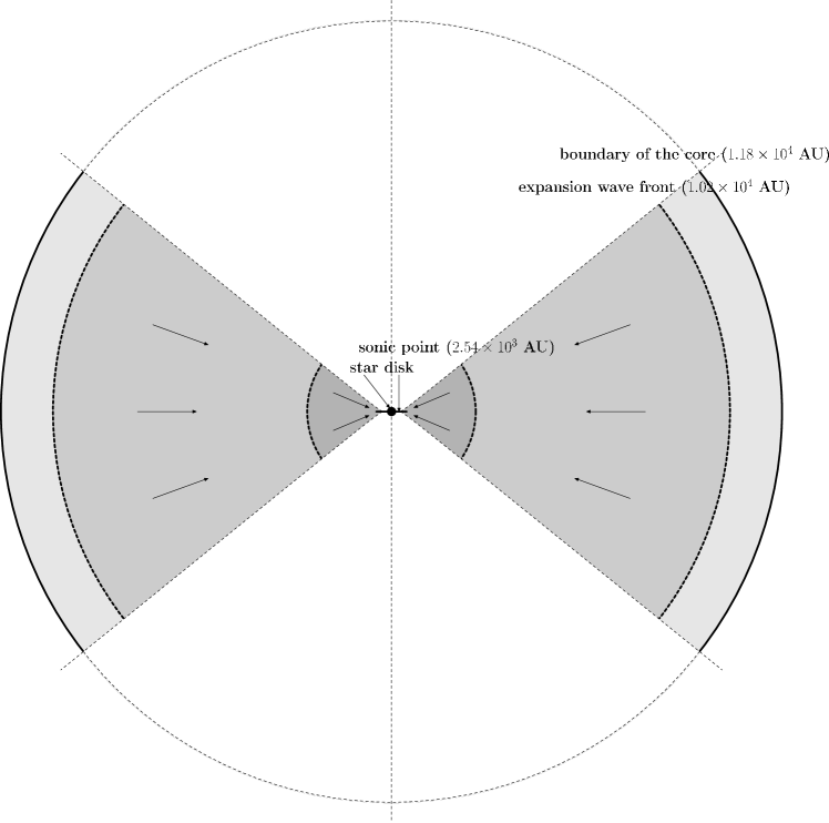
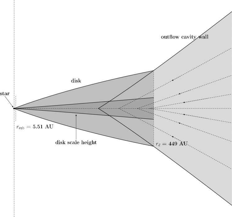
Figure 2.— Structure of the massive star forming core in the fiducial model. The right panel is a zoom-in view of the central region of the left panel. The positions of core boundary, expansion wave front, sonic point (inside which we consider rotation), disk scale height, dust destruction radius and the outer radius of the disk are marked. The outer boundary of the disk is chosen to be a surface with constant density joining the outflow cavity wall at $r_{d}$.

2.4. Protostar

Assuming that the core mass is a constant, the mass of the central protostar indicates its age and evolutionary stage. At some moment, the outgoing expansion wave front will reach the boundary of the core and, depending on the properties of the boundary, may lead to a backward wave and a breakdown of self-similarity. In our case, this happens when the collapsed mass reaches $m_{*d,0}\sim 12\;M_{\odot}$. For the present paper we have chosen to consider a series of models with $m_{*}=8\;M_{\odot}$, and thus a maximum central collapsed mass of 10.67 $M_{\odot}$ for those cases with rotating infall to a disk. Thus the central object is on the verge of becoming a “massive protostar”, following the definitions of Beuther et al. (2007) and Tan (2008). The full evolutionary sequence, including a treatment for greater masses, will be considered in a future paper.

MT03 studied the evolution of massive protostars, and for $m_{*}=8\;M_{\odot}$ and $\Sigma_{\rm cl}=1\>{\rm g\>cm^{-2}}$, the protostar is not expected to have yet contracted to the main sequence. They calculated the values of radius and luminosity of the protostar: $r_{*}=12.05\;R_{\odot}$ and $L_{*}=2.81\times 10^{3}\;L_{\odot}$. For simplicity, we assume a black body spectrum for the star, with surface temperature $T_{*}=1.22\times 10^{4}$ K in this condition. For models with an active disk, we also add the hot-spot luminosity to the stellar spectrum, assuming it is emitted homogeneously from the stellar surface, which means the temperature now is $T_{*,\mathrm{hotspot}}=1.43\times 10^{4}$ K.

For the cases with $\Sigma_{\rm cl}$ = 0.316 g cm^-2, we use the following parameters: $r_{*}=11.3\;R_{\odot}$, $T_{*}=1.25\times 10^{4}$ K, and $T_{*,\mathrm{hotspot}}=1.37\times 10^{4}$ K. For the cases with $\Sigma_{\rm cl}$ = 3.16 g cm^-2, these parameters are: $r_{*}=5.93\;R_{\odot}$, $T_{*}=1.74\times 10^{4}$ K, and $T_{*,\mathrm{hotspot}}=2.62\times 10^{4}$ K.

2.5. Model Series

Table 1Properties of features included in the model series.

Models	Star	Disk	Envelope	Outflow
1	8$M_{\odot}$	no	52$M_{\odot}$, $\rho\propto r^{-1.5}$	no
2	8$M_{\odot}$	no	52$M_{\odot}$, expansion wave	no
3	8$M_{\odot}$	$1/3m_{*}$, thin ($H_{0}/r_{*}=0.01$),	$49.333M_{\odot}$, expansion	no
		passive, $r_{d,\mathrm{in}}=r_{\mathrm{sub}}$	wave, rotation
4	8$M_{\odot}$	as above	only $\sim 29M_{\odot}$ left,	yes
			expansion wave, rotation
5	8$M_{\odot}$	$1/3m_{*}$, thin,	as above	yes
		$r_{d,\mathrm{in}}=r_{\mathrm{sub}}$, active
6	8$M_{\odot}$	$1/3m_{*}$, active, $r_{d,\mathrm{in}}=r_{\mathrm{sub}}$	as above	yes
		thick ($H_{0}/r_{*}=0.1$)
7	8$M_{\odot}$	same as Model 8,	as above	yes
		except $r_{d,\mathrm{in}}=r_{\mathrm{sub}}$
8	8$M_{\odot}$	1/3$m_{*}$, active,	as above	yes
(fiducial)		$H_{0}/r_{*}=0.06$, $r_{d,\mathrm{in}}=r_{*}$

Table 2Parameters of the models comparing different column density.

	Model 8 (fiducial)	Model 8l	Model 8h
mean surface density $\Sigma_{\mathrm{cl}}$ (g/cm2)	1	0.316	3.16
core radius $R_{\mathrm{core}}$ (pc)	0.057	0.10	0.032
position of expansion wave front $r_{\mathrm{ew}}$ (pc)	0.049	0.088	0.028
formation time $t_{f}$ (yr)	$1.29\times 10^{5}$	$3.06\times 10^{5}$	$5.44\times 10^{4}$
position of sonic point $r_{\mathrm{sp}}$ (AU)	$2.57\times 10^{3}$	$4.57\times 10^{3}$	$1.45\times 10^{3}$
outer radius of disk $r_{d}$ (AU)	449.4	801.4	253.4
disk accretion rate $\dot{m}$ ($M_{\odot}$/yr)	$2.398\times 10^{-4}$	$1.035\times 10^{-4}$	$5.667\times 10^{-4}$
stellar radius $r_{*}$ ($R_{\odot}$)	12.0	11.3	5.93
stellar surface temperature $T_{*}$ (K)	$1.22\times 10^{4}$	$1.25\times 10^{4}$	$1.74\times 10^{4}$
stellar + hotspot temperature $T_{*,\mathrm{hotspot}}$ (K)	$1.42\times 10^{4}$	$1.37\times 10^{4}$	$2.62\times 10^{4}$
stellar luminosity $L_{*}$ ($L_{\odot}$)	$2.81\times 10^{3}$	$2.82\times 10^{3}$	$2.84\times 10^{3}$
total accretion luminosity $L_{\mathrm{acc}}$ ( $L_{\odot}$)	$4.90\times 10^{3}$	$2.25\times 10^{3}$	$2.36\times 10^{4}$
disk scale height at stellar surface $H_{0}/r_{*}$	0.06	0.053	0.078

In order to study the effects of all the features discussed above on SEDs and images, we construct a model series starting from the simplest to the one containing all these features. All the models assume an initial core mass of 60 $M_{\odot}$ from which an 8 $M_{\odot}$ protostar has formed at the center.

In Model 1, we assume a spherical symmetric density distribution in the core with a power-law dependence on the radius, $\rho\propto r^{k_{\rho}}$. The total mass in the envelope is $52\;M_{\odot}$ since an $8M_{\odot}$ protostar has already formed at the center.

In Model 2, We change the radial density distribution in the envelope to the expansion wave solution (similar to the thick line in the upper panel of Fig. 1, but here the expansion wave front is at $r=0.0408$ pc and the envelope mass is again fixed at $52\>M_{\odot}$).

We begin to consider rotating infall inside the sonic point and thus a disk around the star in Model 3. The disk is geometrically thin ($H_{0}/r_{*}=0.01$) and passive (no accretion luminosity) with the inner radius set to be the dust destruction radius $r_{\mathrm{sub}}$, which is empirically determined to be (Whitney et al. 2004)

$$r_{\mathrm{sub}}=r_{*}(T_{\mathrm{sub}}/T_{*})^{-2.1}$$ (29)

where $T_{\mathrm{sub}}$ is the dust sublimation temperature and we adopt $T_{\mathrm{sub}}=1600$ K. The expansion wave front now reaches $r=0.0494$ pc for the collapsed mass now is $m_{*}+m_{d}=10.67\;M_{\odot}$. The envelope mass is now $49.33\;M_{\odot}$.

Outflow cavities are added in from Model 4. We keep the density profile in the envelope unchanged, which corresponds to a case that the outflow has just swept up the material to form the bipolar cavities. The envelope mass is now $\sim 29\>M_{\odot}$.

The accretion luminosities (both from disk and hot-spot) are turned on in Model 5. However, since the disk is truncated at the dust destruction radius which in this case is $\sim 98.4\;r_{*}$, most of the disk accretion luminosity is lost and the rest of it ($L_{\mathrm{disk}}=25.29\;L_{\odot}$) is much lower than the hotspot luminosity ($L_{\mathrm{hotspot}}=2.45\times 10^{3}\;L_{\odot}$). Note that in Robitaille model, part of this missing disk luminosity is included in the stellar $+$ hotspot luminosity.

In Model 6 we adjust the disk to be a geometrically thick one ($H_{0}/r_{*}=0.1$) to see the effects of the height of the disk.

In our fiducial model, the disk is extended to the stellar radius so that the accretion luminosity can be conserved. Inside the dust destruction front ($T>1600$ K), gas opacities are used. Here we assume that the $\alpha$-disk model is still valid. The scale height, $H_{0}$, and radial and vertical scaling parameters $\alpha$ and $\beta$ are calculated self-consistently from the assumed opacities and other stellar and envelope parameters: $H_{0}/r_{*}=0.06$, $\alpha=1.75$, and $\beta=1.08$. Fig. 2 is a schematic of the structure in the fiducial model. The positions of core boundary, expansion wave front, sonic point, outer radius of the disk, dust destruction radius, and the scale height of the disk are all marked. Unlike the previous models, in which disk material can exist at any height (though the density is very low at large $z$), we truncate the disk at a fixed density of $2\times 10^{-15}\;\mathrm{g}\;\mathrm{cm}^{-3}$ so that the disk atmosphere joins smoothly with the infalling envelope. (The input density profile can be seen in the lower panel of Fig. 3.) We expect that the existence of optically thick gas in the innermost region of the disk can make a significant difference. In order to investigate this effect, we construct Model 7 to be the same as the fiducial model except without gas disk ($r_{d,\mathrm{in}}=r_{\mathrm{sub}}$). And the fiducial model is labeled with Model 8. Table 1 lists the differences of all these models.

The column density of the clump where the core is embedded in can affect the surface pressure of the core, therefore its size, outer radius of the disk, accretion rate and also the scale height of the disk. In order to investigate this effect, we consider other two values for the mean surface density of the clump, $\Sigma_{\mathrm{cl}}=0.316$ and 3.16 g/cm². These correspond to a change in column density of the core by a factor of 10 and the surface pressure by a factor of 100. These two models are labeled with Model 8l (low surface density) and 8h (high surface density). Table 2 lists the differences of these three models.

3. Simulations

Figure 3.— Input temperature and density for our fiducial model. $n_{\mathrm{He}}=0.1n_{\mathrm{H}}$ is assumed here. The black contours in the upper panels correspond to the dust destruction front (1600K), cells inside which are assigned with gas opacities. The white contours show the photon-diffusive region calculated in the fiducial model, a photon emitted inside which will move to the surface through a path with constant $r$ and emitted again from the surface. The temperatures of the cells on that path are calculated with grey atmosphere approximation, which is why the the dust destruction fronts have these vertical structures. Also, since the frequency of the photon, when it finally leave the photon-diffusive region, is calculated from the surface temperature, these vertical structures inside it should not affect the results.

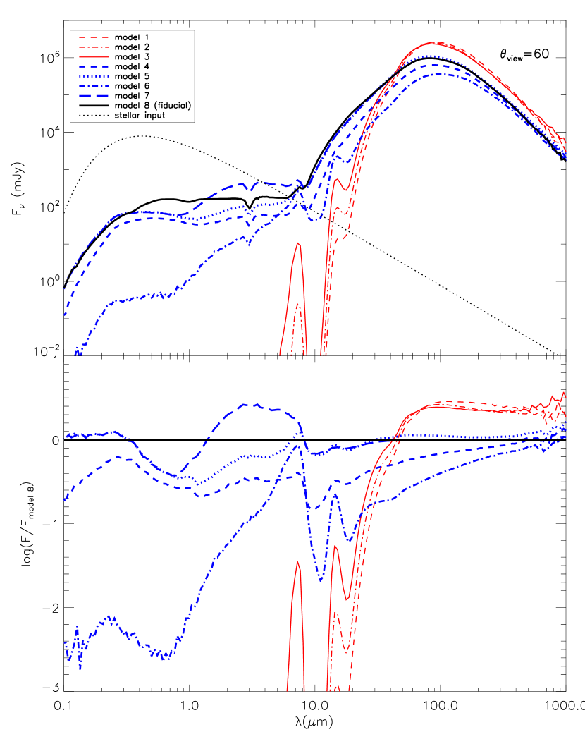
Figure 4.— SEDs for the model series, assuming a distance of 1 kpc. A typical inclination of $60^{\circ}$ is chosen. The upper panel shows the SEDs and the lower panel shows the differences of each model from the fiducial one. The black solid curve is for the fiducial model, the red thin curves are for Model 1 - 3 (models without outflow cavities), and the blue thick curves are for Models 4 - 7 (models with outflow cavities) The black dotted line is the input stellar spectrum (black-body) which is used for all the models.

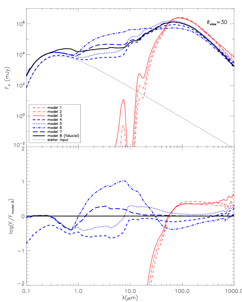
Figure 5.— The same as Fig. 4, except for an inclination of $30^{\circ}$.

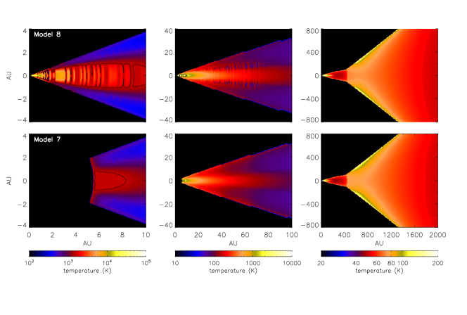
Figure 6.— Output temperature distribution of Model 7 and 8, showing the difference the gaseous innermost disk makes. The black contours are dust destruction front ($T$=1600K).

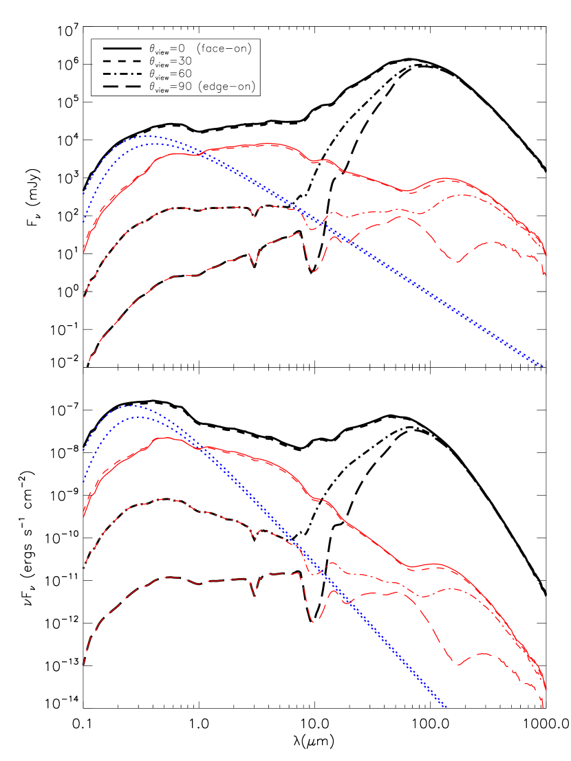
Figure 7.— SEDs of the fiducial model (Model 8) at 4 inclinations, assuming a distance of 1 kpc ($F_{\nu}$ in upper panel and $\nu F_{\nu}$ in lower panel). The thicker lines are total fluxes and the thiner red lines are only the scattered light. The lower dotted blue line is the input stellar spectrum (black-body). The upper dotted line is the total luminosity of star and hot-spot emitted as a black-body.

We use the Monte Carlo radiation transfer code by Whitney et al. (2003b) to perform our calculations. This code includes thermal emission, non-isotropic scattering and polarization due to scattering from the dust in a spherical-polar grid, using the method of Monte Carlo radiative equilibrium by Bjorkman & Wood (2001). This method requires that the opacities are set up at the beginning of each run and kept unchanged. During the run, the temperature in each cell is always being corrected by calculating the balance of absorption and emission of new photon packets. This becomes a problem when gas opacities are included because they are highly dependent on the temperature and density. So we have to iterate to obtain the correct temperature profile for the disk (especially for the inner region) and then use it to set up opacities for each cell.

We choose the analytical temperature profile from $\alpha$-disk model in our case as an initial condition. After several iterations, the temperature of the outer disk $\gtrsim$ 4 AU becomes quite stable. However, because of the discontinuity of the opacities at the transition region between gas and dust, the temperature profile in the inner region oscillates between two phases. Even though the difference can be large between results from two adjacent steps (i.e. $T_{n}(r,\theta)$ and $T_{n-1}(r,\theta)$), the averaged temperature profile of two adjacent step should keep similar (i.e. $\log(T^{\prime}_{n}(r,\theta))=(\log(T_{n}(r,\theta))+\log(T_{n-1}(r,\theta)))/2$). So we stop the iteration when $T^{\prime}_{n}\sim T^{\prime}_{n-1}$, more specifically, when standard deviation of the distribution of $({\rm log}T^{\prime}_{n}-{\rm log}T^{\prime}_{n-1})/{\rm log}T^{\prime}_{n}$ for the cells inside 4 AU becomes consistently $<0.1$, which corresponds to a variation of $\sim$ 25%. Then we use the temperature profile which is higher in the midplane to be the input for the final run with large number of photons to generate SEDs and images. We performed simulations with both input temperature profiles and saw no significant differences on the SEDs and images. We also doubled the photon number for the iteration but found no significant dependence of the standard deviation on the photon number. It should be noted here that 0.1 standard deviation inside 4 AU is only an arbitrary standard. The upper panel of Fig. 3 shows the input temperature profile. The black contours correspond to the dust destruction front ($T=1600$ K), inside which gas opacities are assigned depending on the temperature and density. We can also see that the dust destruction front extends to $\sim 10$ AU in the midplane and $\sim 3$ AU on the surface of the disk, which agrees with the estimate of the dust destruction radius of 5.5 AU in Model 3 - 7. We note that temperature iteration is only used in Model 8, while in other models, the dust opacities are assigned only depending on the region and the density. Also, this input temperature is only used to assign opacities. It is not the initial temperature condition for each run.

The inner region of the disk around the midplane is very optically thick and so detailed radiative transfer simulation becomes very time-consuming. Thus in the code the grey atmosphere approximation is used to describe this region (photon-diffusive region). A photon generated inside this photon-diffusive region will move to the surface of the region by following a path with same $r$, and is then emitted with a frequency calculated based on the temperature of the surface cell. The temperatures of the cells on that path are calculated accordingly with the grey atmosphere approximation. In models except the fiducial one (Model 3 - 7), as in the original code, a cell is set to be in the photon-diffusive region if the optical depth from $z=\infty$ to it is larger than 10. In the fiducial model, we change this to a more restrictive local definition, that the photon-diffusive region is where the mean free path is smaller than 0.1 $H(r)$. Note that as long as this photon-diffusive region is set small enough, it should not affect the final results.

A 3000 $\times$ 1499 grid is used to resolve the $r\times\theta$ space. In $r$ space, $\sim 600$ cells are used to resolve the disk with a finer grid in inner region, $\sim 150$ cells are used to cover the region inside $\sim 6$ AU in the fiducial model. In $\theta$ space, the grid is finer in the disk (especially around the midplane) and around the opening angle of the outflow cavity $\theta_{w,\mathrm{esc}}$. $\sim 700$ cells are used between $20^{\circ}$ above and below the disk midplane and $\sim 300$ cells are used between $50^{\circ}$ and $53^{\circ}$ ($\theta_{w,\mathrm{esc}}=51^{\circ})$.

For each run, SEDs at ten inclinations (evenly distributed in cosine space) can be produced simultaneously, while if the “peeling-off” mode is used, images and SEDs with higher signal-to-noise ratio are produced for the particular “peeling-off” angle. The “peeling-off” mode is very time-consuming. For most of our models, $10^{8}$ photons are used in one run, and it typically takes several days to one week running on a single processor. This number of photon packets is still not perfect for an image of the whole core, especially for those at wavelengths with low fluxes. Because this code does not enable parallel computing now, in order to save time, for each model we run 10 times with different random seeds simultaneously on different processors, and superposed their results, making our final images contain $10^{9}$ photons.

Images are produce at several wavelengths and convolved with filter functions for comparison to observations. The code has already included filters such as Spitzer IRAC filters at 3.6, 4.5, 5.8 and 8.0 µm, Spitzer MIPS filters at 24, 70 and 160 µm, and 2MASS J, H, K bands. We also add in the filters of GTC-CanariCam, Herschel PACS and SPIRE, and SOFIA FORCAST. We will show images both before and after convolution with resolution of these particular instruments.

3.1. Dust Opacity

We use three dust grain models for different regions: (1) the envelope; (2) lower density regions of the disk, and (3) the densest regions in the disk ($n_{\mathrm{H}_{2}}>10^{10}\;\mathrm{cm}^{-3}$, the criterion used by Robitaille et al. 2006). For our present models there is no dust (or gas) in the outflow cavities. The default dust models in the code are used without any change (Whitney et al. 2003a).

The dust model used in the envelope is based on that derived by Kim et al. (1994) for the diffuse interstellar medium (ISM). The size distribution is modified by Whitney et al. (2003a) to fit an extinction curve typical of the more dense regions of the Taurus molecular cloud with $R_{V}=4$. These grains also include a water ice mantle covering 5% of the radius. For the lower density regions of the disk, the grain model of Cotera et al. (2001) is used. It has grains larger than ISM grains, but not as large as the disk midplane grains.

For the densest regions of the disk, we use the dust model with large grains ($\sim$1 mm; model 1 in Wood et al. 2002), which fit the HH 30 disk SED well. Compared to ISM grains, the larger dust grain model has a shallower wavelength-dependent opacity: lower at short wavelengths and larger at long wavelengths.

3.2. Gas Opacity

For most regions of the disk, dust grains dominate the opacity, even if the mass ratio between dust and gas is low (0.01 is used in our models). However, in the innermost region of the disk, where the dust cannot exist ($T>1600$ K), opacity is dominated by gas. Especially when the temperature is high ($\sim 10^{4}$ K), the mean opacities of the gas can be comparable or higher than dust opacities. As discussed in Section 2.2, most of the disk accretion luminosity is from this innermost region. Thus, gas opacity should be included in a realistic model.

In order to simulate the frequency of each photon packet emitted from the gas-dominated region correctly, not only Rosseland or Planck mean opacities, but also the frequency-dependent opacities are needed. Besides, the gas opacity is highly dependent on the temperature and the density, which make our problem much more complicated. Since our aim is only to simulate the disk emission correctly, especially in near and mid-IR, rather than to simulate the details of line profiles, we smooth the monochromatic opacities for simplicity and smaller memory demand. Also, we assign opacities to a grid in temperature and density, rather than to interpolate to obtain opacities at exact temperature and density.

For temperatures higher than $\sim 3000$ K, we adopt gas opacities from OP project (Seaton et al. 1994, Badnell et al. 2005 and Seaton 2005). They provide monochromatic gas opacities of hydrogen, helium and other 15 elements, in large ranges of temperature ($\sim 3000$ K to $10^{8}$ K, we only use those of temperature up to $\sim 10^{6}$ K in our present model since the maximum temperature we can reach in the models is less than this) and density. The opacities are mainly due to the line absorption, ionization, H^- bound-free absorption, electron-hydrogen/helium free-free absorption. For scattering, Thompson scattering with a collective effect is considered (Boercker 1987). For regions with $T<3000$ K, the opacity model of Alexander & Ferguson (1994) is adopted. However, they do not provide monochromatic opacities for a range of temperatures and densities. So we use the monochromatic opacities shown in Fig. 4 of Alexander & Ferguson (1994) which is for a temperature of 2000 K and a density of $8\times 10^{-12}\;\mathrm{g/cm}^{3}$, and rescale it for other temperatures and densities based on their Rosseland mean opacities. Fortunately, the temperature range for this model is quite narrow (1600K - 3000K). Alexander and Ferguson’s model includes both gas and molecules. At $\sim 2000$K, the total opacity is dominated by molecules, especially H₂O and TiO. Atomic lines and CO lines are important at some wavelengths. Other continuous sources include H^- absorption and Rayleigh scattering of H and H₂.

In this way we construct an opacity grid of temperature and density. The temperature varies from 1600 K to 10⁶ K with an interval of 0.1 in logarithmic space, and the density varies from $\sim 10^{-8}$ to $\sim 10^{-15}$ g/cm³ with an interval of 0.5 in logarithmic space. For each $T$ and $\rho$, a monochromatic opacity file is assigned, so that we have totally 148 gas opacity files in our present model. At the beginning of each run, a temperature profile is read in, and in each cell the gas opacity file with closest $T$ and $\rho$ to the read-in values is chosen. The opacities are not changed during the calculation.

Since here we are not concerned with line absorption and emission, it is better to smooth the monochromatic opacities to save computing memory. In the code, three important values are calculated: 1) Rosseland mean opacity

$$\frac{1}{\kappa_{\mathrm{R}}}=\frac{\int_{0}^{\infty}(\partial B_{\nu}/\partial T)/\kappa_{\mathrm{ext}}(\nu)\mathrm{d}\nu}{\int_{0}^{\infty}(\partial B_{\nu}/\partial T)\mathrm{d}\nu},$$ (30)

used to determine the photon-diffusive region inside the disk; 2) Planck mean opacity

$$\kappa_{\mathrm{P}}=\frac{\int_{0}^{\infty}\kappa_{\mathrm{abs}}(\nu)B_{\nu}\mathrm{d}\nu}{\int_{0}^{\infty}B_{\nu}\mathrm{d}\nu},$$ (31)

used to calculate the energy equilibrium in a cell; and 3)

$$P_{\nu}=\int_{0}^{\nu}\frac{\kappa_{\mathrm{abs}}(\nu)}{\kappa_{\mathrm{P}}}\frac{\partial B_{\nu}}{\partial T}\mathrm{d}\nu,$$ (32)

where $P_{\nu}$ is the probability that a photon packet is emitted from a cell with a frequency between 0 and $\nu$ (Bjorkman 1997). For $\kappa_{P}$ and $P_{\nu}$ it is best to smooth opacities with linear averaging, thus giving better estimates of equilibrium temperatures and photon frequencies. However, this method tends to increase $\kappa_{R}$ by $\sim$10% or more. Averaging ${\rm log}\kappa$ reduces the importance of line absorption and yields more accurate Rosseland mean opacities. For our problem, the precise location of the boundary of the photon-diffusive region is is not very important, so we smooth opacities with linear averages. The original gas opacity files contain $10^{4}$ frequencies between $h\nu/kT=0.001$ and 20. We smooth them by averaging 50 adjacent frequencies.

4. Results

4.1. SEDs

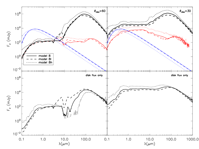
Figure 8.— SEDs of Model 8 ($\Sigma_{\mathrm{cl}}$= 1 g/cm²), Model 8l ($\Sigma_{\mathrm{cl}}$= 0.316 g/cm²) and Model 8h ($\Sigma_{\mathrm{cl}}$= 3.16 g/cm²) at inclinations of $60^{\circ}$ (left panels) and $30^{\circ}$ (right panels), assuming a distance of 1 kpc. For each inclination, the upper panel shows the total fluxes (black), scattered fluxes (red) and stellar input (blue), while the lower panel shows fluxes from the disk only.

4.1.1 SEDs of the Model Series

Figures 4 and 5 show the SEDs of the model series at inclination angle between our line of sight and the protostar rotation axis of $60^{\circ}$ (i.e. a more equatorial view) and $30^{\circ}$ (i.e. a more polar view) respectively. In each figure, the upper panel shows the total fluxes while in the lower panel these SEDs are compared to the fiducial model (Model 8). The $\theta=60^{\circ}$ line of sight goes through the envelope material, in which case the photons from the protostar and the disk are all reprocessed by the dust before they can escape the core. The $\theta=30^{\circ}$ line of sight from the central star passes through the outflow cavity (for Model 4 - 8), in which case we can see the stellar black-body spectra in the short wavelength region of the SEDs. Some important features in the SEDs include the water ice feature at 3 µm and silicate features at 10 µm and 18 µm. The ice feature is only present for the higher inclination view for which the lines of sight pass through the envelope material, which uses a dust model with ice mantles.

Models 1 to 3 show very similar SEDs, where we do not see any radiation at short wavelengths. The 10 µm silicate features are all very deep. The occurrence of the expansion wave (Model 2) and rotation/disk (Model 3) shift the far-IR peak a little to shorter wavelengths, and increases the mid-IR emission, making the 18 µm silicate feature deeper. This is because the expansion wave and the Ulrich solution decrease the density of the inner region of the core, and thus reduce the extinction. For Model 3, which is not spherically symmetric, the SEDs do not show much difference between the different inclinations. It should be noted that in Model 3 rotation is only considered inside the sonic point. In a more realistic solution, the material in the outer region of the envelope would also be redistributed by the effect of the rotation (like the solution of Terebey et al. (1984) for an isothermal core) so that one might see larger differences.

The outflow cavities change the shape of SEDs significantly. With outflow cavities (Model 4 to 8), the SEDs show a large excess at wavelengths shorter than 10 µm. The position and height of the far-IR peak and the 20 µm $\sim$ 70 µm slopes are affected by the cavity as well. Especially for a low inclination, the star and disk can be seen directly. The fluxes at wavelengths shorter than 10 µm are larger than those at a high inclination by about two orders of magnitude. Note that the short wavelength emission seen in the $\theta=60^{\circ}$ view is essentially all due to scattered emission from the outflow cavity walls.

Compared to a passive disk, an active disk with accretion luminosity increases the fluxes at all wavelengths without many changes in the shape of the SEDs (comparing Model 4 and 5). The accretion luminosity in Model 5 is mainly due to the hot-spot, while most of the disk accretion luminosity is lost here because of the absence of the innermost disk. The total energy is conserved only in Model 8, which the disk is extended to the stellar surface.

The effect of the thickness of the disk is distinct on the SEDs (comparing Model 5 and 6). A thicker disk tends to obscure more photons at high inclinations and emit or scatter them to low inclination directions - i.e. more flux escapes via the outflow cavities. Therefore, with a thicker disk, Model 6 at $\theta=30^{\circ}$ shows a rise between 1 and 10 µm which even smooths out the far-IR peak, while at $\theta=60^{\circ}$ the SED shows a decrease in near-IR and shorter wavelengths, and a deeper silicate features.

Model 8 shows how the SED changes by including the flux from the innermost disk region. Compared to previous models, the optical and near-IR emission is significantly increased, in both high and low inclinations. Model 7 has exactly the same geometry and density setup as Model 8, except that it has a disk truncated at $r_{\mathrm{sub}}$. The opacities are chosen depending on the input temperature and density in Model 8 while in Model 7 they only depend on the density, therefore, even outside $r_{\mathrm{sub}}$ the opacity setup of these two models can be different. Because of the truncated disk, the majority of the disk accretion luminosity is lost in Model 7. This missing luminosity shows up in Model 8 mainly as optical radiation. However, the near-IR flux in Model 8 is not so bright as Model 7. The far-IR SEDs of these two models do not show much difference.

Fig. 6 shows the final output temperature distributions of these two models. The temperature of the disk reaches $\sim 10^{5}$ K at the innermost region in Model 8, while the highest temperature in Model 7 is only $\sim 3000$ K. This explains the optical excess in the SED of Model 8. However, the existence of the innermost disk shields the flux from the star, therefore in Model 7 the temperature at the surface of the disk and the base of the outflow cavity becomes higher, leading to the higher near-IR flux on the SED. For the models presented here, we do not have any material in the outflow cavity. If any dust grain exists there, the optical emission in Model 8 will be suppressed and the disk luminosity may appear as more near- and mid-IR radiation. This will be examined in a future paper.

4.1.2 SEDs of the Fiducial Model

Fig. 7 shows the SEDs of our fiducial model (Model 8) at four inclinations. Even after we smoothed the monochromatic opacity curves of gas, the original output SEDs still show some significant emission features, mainly H$\alpha$. Since the line profile is not exactly correct in our models and it is not the interest of our present study, we subtract the H$\alpha$ feature and smooth out other line features with wavelengths $<2$ µm. The energy contained in the H$\alpha$ line is typically $\lesssim$ few%.

The SEDs at 4 inclinations are shown here, from a view along the rotation/outflow axis to that through the disk plane. The inclination of the viewing angle changes the observed flux at short wavelengths significantly. It also affects the height and position of the peak in the far-IR region, and the mid-IR spectral slope. The SED at wavelengths longer than $\sim$100 µm is not affected by the inclination. Inclinations of $30^{\circ}$ and $0^{\circ}$ have very similar SEDs ($0^{\circ}$ inclination contains 8% more energy than $30^{\circ}$ inclination). Recall, the outflow cavity has an opening angle of $51^{\circ}$, which means we can directly see the star in both these cases. The stellar spectrum and the black-body spectrum containing both stellar and hot-spot luminosity are shown by the dotted lines. Their difference shows the luminosity from the hot-spot region. From high inclinations to low inclinations, because of the change of the optical depth, the silicate feature change from a big absorption feature to a weak emission feature.

The dashed lines show the SEDs of only scattered light. At high inclination angles, the observed light at short-wavelengths has always been scattered, while at low inclinations, we can see stellar radiation and thermal emission from the disk. In the far-IR, the flux is dominated by the thermal emission of the envelope. Such significant difference between low inclinations and high inclinations is partly because we have an empty outflow cavity.

4.1.3 Effect of Different Mass Surface Density

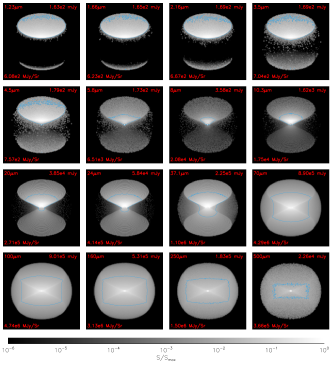
Figure 9.— Images for the fiducial model at inclination of $60^{\circ}$, assuming a distance of 1 kpc, at different wavelengths. Each image has 149 $\times$ 149 pixels, and field of view of 30” $\times$ 30”. Each image is normalized to its maximum surface brightness which is labeled in the bottom-left corner. The values on the top-right corners are the total fluxes. The blue contour is 1% of the maximum surface brightness

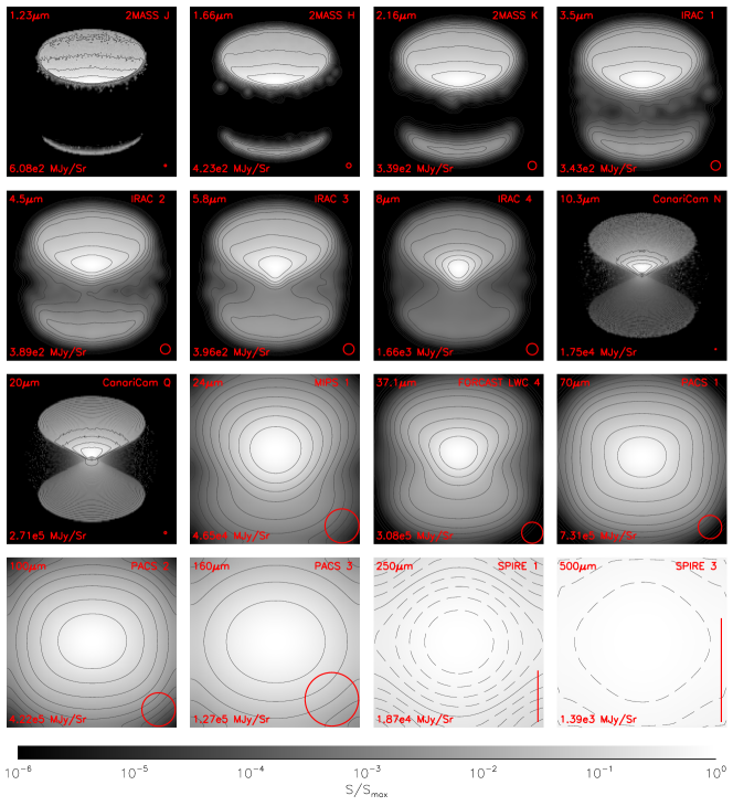
Figure 10.— Same as Fig. 9, except convolved with the resolution of each particular instrument, labeled in the top-right corner and shown as red circles of radius equal to the HWHM (or line segments with lengths equal to the HWHMs for Herschel SPIRE) on the bottom right corners. The maximum surface brightness (which is dependent on the resolution) is labeled in the bottom-left corner. The contours for most of the images have intervals of half an order of magnitude from the maximum brightness. Because some images (1.23, 10.3 and 20 µm) are relatively noisy at faint fluxes, only five contours with intervals of half an order of magnitude are shown here. For images at 250 and 500 µm, dashed contours have intervals of 0.1 dex.

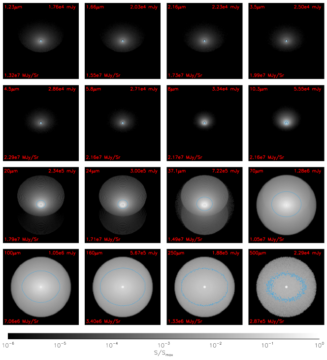
Figure 11.— Same as Fig. 9, except at inclination of $30^{\circ}$.

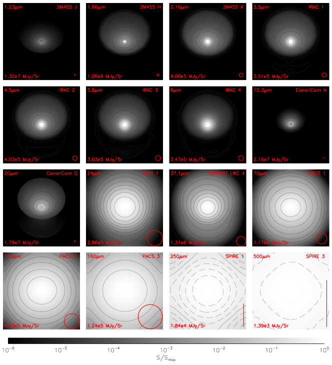
Figure 12.— Same as Fig. 10, except at inclination of $30^{\circ}$ and that for images at 1.23, 10.3 and 20 µm, only five contours with intervals of an order of magnitude are shown.

Figure 13.— Flux distribution along the projected outflow axis. Fluxes are normalized by the mean value of a narrow strip across the core along the axis. Different curves show different wavelengths. The upper panel is at inclination of $60^{\circ}$ and the lower panel is at $30^{\circ}$.

Model 8, 8l and 8h compare the effect of different mean surface densities of clump in which the core is embedded, which affects the surface pressure of the core, and therefore the size of the core, the accretion rate, the disk structure and the protostar evolution. The size of the core, the radius of the expansion wave front, the position of the sonic point and the disk radius are all proportional to $\Sigma_{\mathrm{cl}}^{-1/2}$, so with higher clump surface density, the core is more compact and accordingly the accretion rate is higher. The scale hight of the disk is also larger in the high $\Sigma_{\mathrm{cl}}$ case. The stellar luminosities of these three models are similar but Model 8h has a much bluer stellar spectrum, because of the higher hot-spot accretion luminosity. Some important parameters of these three models are listed in Table. 2

Fig. 8 compares SEDs of these three models at both $60^{\circ}$ and $30^{\circ}$. As discussed above, higher surface density leads to higher bolometric luminosities, which can be seen from the SEDs: At inclination of $30^{\circ}$, with a higher surface density, the flux is higher at all wavelengths; And at $60^{\circ}$ inclination we can see the same effect in optical, near-IR and far-IR emissions. However, in mid-IR, Model 8l shows a rise of the flux and a very significant 10 µm silicate feature, while the other two models do not. To explain this, we also show the disk flux in the lower panels. Here, disk flux contains photons which have their last emission in the disk, and then either escape the core directly or are scattered before they reach the observer. At the inclination of $60^{\circ}$, the disk is blocked by the envelope. The short-wavelength fluxes from the disk should all have been scattered. They keep the trend that the model with higher surface density has higher fluxes. However, in mid- and far-IR, the fluxes should have suffered the extinction of the envelope, making the model with higher surface density have lower fluxes because of the higher extinction. Thus, even though Model 8 and 8h have very strong silicate features in their disk SEDs, they are buried in the envelope fluxes in the total SEDs, while Model 8l shows the high disk flux level in mid-IR and a significant silicate absorption feature because of its lower extinction and lower envelope flux.

4.2. Images

4.2.1 Images of the Fiducial Model

Fig. 9, 10, 11 and 12 show the images for the fiducial model (Model 8) at inclinations of $60^{\circ}$ and $30^{\circ}$, assuming a distance of 1 kpc and no foreground extinction. The instruments filters chosen here are: 2MASS J, H, K bands, Spitzer IRAC 3.5 µm, 4.5 µm, 5.8 µm and 8 µm, MIPS 24 µm, GTC-CanariCam N band and Q wide band, SOFIA FORCAST 37.1 µm, Herschel PACS 70 µm, 100 µm, 160 µm, and SPIRE 250 µm and 500 µm. We show both resolved images and those after convolving with PSFs of the particular instruments. Images showed here are all normalized to their maximum surface brightnesses which are labeled on each image. $10^{9}$ photon packets are used. However they are still not enough to produce a smooth image for the narrow filters or at the wavelengths with low fluxes. Besides, the simulation grid also contributes to this problem, like the strip patterns in the images at some wavelengths (e.g. 20 µm). Around the opening angle of the outflow cavity, the grid with very small change of the polar angle intersects with the cavity wall at quite different radii. Even we have made the grid much finer in polar angle at the region around the cavity wall, these patterns can still be seen, especially at outer regions of the envelope. A finer grid would demand more memory and computing time.

On the images at inclination of $60^{\circ}$ before convolution with the instrument PSF, the most significant features are the outflow cavities. They can be seen in any wavelength, though they become not so obvious in far-IR wavelengths where the thermal emission of the envelope dominates. At this inclination, the line of sight intersects with the envelope, thus in near-IR the only emission we can see is scattered by the cavity wall and escapes from the opening region, especially from the side facing us. Deeper regions appear as the wavelength increases. The central protostar and disk begins to show up in mid-IR images. The dark lane around it shows the size of the disk. In the mid-IR, the cavity walls dominates the emissions, as has been discussed by De Buizer (2006). Both sides can be clearly seen and the brightest region is the base of the cavity. The emission of the envelope takes over at longer wavelengths, making the image symmetric and the outflow cavity begins to fade. The central star and disk can still be seen as the brightest region in those wavelengths.

At the inclination of $30^{\circ}$, the central object can always be seen through the empty outflow cavity. At shorter wavelengths, only the side facing us of the cavity is significant and the opposite side is very dim. Far-IR emission is dominated by the envelope and it is hard to tell the features of the cavities. It should be noted here, especially when comparing the 30^∘ and 60^∘ images, that the images are all scaled to their maximum surface brightness, which is generally much greater for the 30^∘ viewing angles.

After convolving with PSF of particular instruments, in the far-IR, the contours become very symmetric and we cannot tell the inclination or the opposite outflow cavities. It is possible to see the opposite outflow in MIPS 24 µm and FORCAST 37.1 µm at high inclinations, if the S/N is large enough. The two sides of the outflow cavities are clear in IRAC images and in near-IR images. GTC-CanariCam has very high resolution so it may enable us to see the central region in mid-IR.

Fig. 13 shows the flux profile along the system axis at inclinations of both $60^{\circ}$ and $30^{\circ}$. Each profile is normalized by the mean flux of a very narrow strip along the axis across the whole core. Thus, the general shape and level of the profiles are independent on the resolution of the image. But the curve would be smoothed out if a larger PSF-FWHM is used. At inclination of $60^{\circ}$, as we discussed above, at short wavelengths, the central region is totally blocked by the envelope, most of the emission comes from the outflow cavity. In the mid-IR, the maximum surface brightness comes from the base of the outflow cavity rather than central star and disk, on the side the outflow cavity is opposite to us, the flux drops very fast by almost four orders of magnitude, while on the side the outflow is facing us the flux drops much more gradually. In the far-IR, the profile is symmetric on both sides, and central region has the maximum surface brightness. At lower inclination, the maximum flux always comes from the center. In the far-IR, the profile is very similar to the case in higher inclination. At shorter wavelengths, the contrast between outer regions and the center point is much higher than the previous case, so that the profile drops very fast. At 1.66 µm and 10.3 µm we can only see the flux due to the outflow cavity facing us, while the other side only shows up at 20 µm. Because in our models it is empty outside the core, the profiles all cut off at the core radius, which is not true in reality since clump material can extend to larger radii.

4.2.2 Effect of Different Surface Density

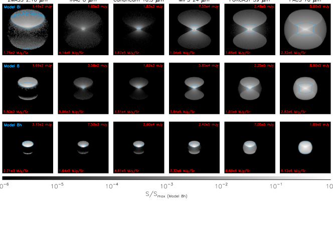
Figure 14.— Images for Model 8, Model 8l and Model 8h at the inclination of $60^{\circ}$, assuming a distance of 1 kpc. The size of the image is 50” $\times$ 50”. The resolution here is set to be 0.5”, so the surface brightnesses can be compared. Each images are scaled to the maximum brightness of Model 8h at that band, but their own maximum brightness is also labelled in the bottom-left corners. The total flux in each image is also labelled in the top-right corner. The blue contour is 1% of the maximum surface brightness in that image.

Fig. 14 compares the images of Model 8, 8l and 8h at 6 wavelengths. The size of the images are all 50”$\times$50”. We can see that the core is smaller when the surface pressure is higher. The surface brightness is dependent on the resolution, so here we convolved all images with same PSF with FWHM of 0.5”. The images are scaled to the maximum surface brightness of Model 8h at each wavelengths, so the brightnesses of the three images at each wavelength can be directly compared.

The total fluxes and the maximum surface brightness in images of Model 8h are generally higher than those of the other two models. This is natural since the total luminosity is much higher in this model. The optical depth is larger when $\Sigma_{\mathrm{cl}}$ is higher. In the near-IR, we can see the base of the outflow cavity facing us and most of the opposite side in Model 8l, while we can only see the light from the opening region of the cavities in Model 8h. The central region shows up in Model 8h only in far-IR, while it can be seen at mid-IR in Model 8 and 8l. With lower surface density, the contrast between two sides of the outflow cavities becomes smaller. In Model 8h the side towards us is much brighter than the other side, even at 70 µm, while the other two models show almost symmetric images. We can also see that the mid-IR emission is dominated by the cavity walls, especially in the cases with higher extinction, as opposed to that with lower extinction the emissions are more concentrated to the central region.

5. Discussions and Conclusions

We have constructed a model for individual massive star formation, with a $60\;M_{\odot}$ initial core that forms an $8M_{\odot}$ protostar. We included the inside-out expansion wave in the core, free-fall rotating collapse in the inner region, an accretion disk of 1/3 the mass of the star, and bipolar outflow cavities with large opening angle, parameters of which are all calculated self-consistently. For the first time, we considered an optically thick inner disk with gas opacities which were assigned depending on the pre-calculated temperature profile. This inner disk enabled us to calculate the emission from the active disk with correct total luminosity and spectrum.

Compared to the Robitaille model, our parameter space covers higher accretion rates, higher disk mass, denser envelopes and larger outflow cavities. Also, in the Robitaille model the disk accretion luminosity is much lower than that in our model since the disk is truncated at the dust destruction radius, while the hot-spot luminosity on the stellar surface is set to be $Gm_{*}\dot{m}(1/r_{*}-1/r_{\mathrm{co}})$ where $r_{\mathrm{co}}$ is the magnetic co-rotation radius and set to be $5r_{*}$, making the hot-spot luminosity is 4/5 of the total accretion luminosity $L_{\mathrm{acc}}$. So energy of $\lessapprox 0.2\;L_{\mathrm{acc}}$ is lost. In our model, the total accretion luminosity is divided equally into disk accretion luminosity (emitted from the disk extended to stellar radius with gas and dust opacities) and hot-spot luminosity (added on the stellar spectrum). Also, the Ulrich solution is used for the whole envelope in Robitaille model, which means the whole envelope is assumed to be free-falling and the infalling rate is constant at all radii. As discussed in Section 2.1.3, the core undergoes free-fall only in the inner region. Therefore, for a given core mass and accretion rate, our model has a more compact core with higher extinction, causing the far-IR peak of the SED to be at lower fluxes and at longer wavelengths.

We have presented SEDs of the model series, the fiducial model, and the models with higher and lower surface pressure, at typical inclinations. We also have presented images for the fiducial model at JHK bands, IRAC and MIPS bands, GTC-CanariCam bands, SOFIA bands and Herschel bands, both resolved and convolved with the resolutions of each instrument. The main conclusions can be summarized as:

1. Outflow cavities affect the SEDs significantly and cause a large difference between low and high inclinations of our viewing angle. However, the present modeling assumes these cavities are optically thin, which may not be valid, especially at the shorter wavelengths. This issue will be investigated in a follow-up paper. The height of the disk also affects the SEDs. With a thicker disk, the near- and mid-IR fluxes at low inclinations become higher, while at high inclinations it suppresses the fluxes (especially at short wavelengths) and creates deep silicate features. Also, the density distribution in the core (especially the inner region) can affect the mid-IR flux levels, the silicate features, and the far-IR peaks.

2. The temperature of the innermost region of the disk can reach $\sim 10^{5}$ K. The disk becomes optically thick in such conditions even if no dust can exist there. SEDs show the rise of optical emission due to this hot inner disk. This optically thick inner disk also shields flux from the protostar, leading to lower temperatures on the surface of the disk and the base of the cavity wall, and therefore lower fluxes in near-IR and mid-IR part of the SEDs.

3. The SEDs of the fiducial model show that the inclination can affect SEDs at wavelengths shorter than 100 µm, including the far-IR peak. The mid-IR spectral slope changes significantly with inclination. The silicate feature changes from a deep absorption feature to an emission feature from high inclinations to low inclinations, due to the change of the optical depth.

4. With higher surface pressure, the core becomes more compact and the accretion rate and luminosity become higher, leading to higher fluxes at all wavelengths (except in the mid-IR for high inclination cases which suffer higher extinction). High extinction can also cause the mid-IR flux to be dominated by the envelope, and thus hide the silicate absorption feature. Thus, only in the model with low extinction does the silicate absorption feature show up.

5. Outflow cavities are the most significant features on the images, except at wavelengths longer than 70 µm. At inclinations of $60^{\circ}$, from short wavelengths to long wavelengths, the brightest point moves from the outer region of the cavity to the base of the cavity wall, and to the center of the core in far-IR, while at inclination of $30^{\circ}$, it is always the central region. At inclination of $60^{\circ}$, the opposite outflow cavity can be seen n the mid-IR if fluxes $\sim 10^{2}-10^{3}$ times fainter than the peak can be probed. It is very difficult to see the opposite cavity at an inclination of $30^{\circ}$. GTC-CanariCam (and other 10 m class telescopes with mid-IR cameras) has very high angular resolution so it may enable us to resolve the central disk system. The flux distribution along the outflow axis can help constrain model assumptions and inclination angles and so will useful to measure. In the mid-IR, the cavity walls seem to dominate the emission, but for lower density cores with lower extinction, the central region becomes brighter. The contrast between the two sides of the outflows in mid- and far-IR increases as the extinction becomes higher.

The model we have presented will be improved in future papers by a detailed consideration of the effect of including gas and dust in the outflow cavity. Currently models for the density distribution here are quite uncertain, which is why we defer this study to a future date. An evolutionary sequence of protostellar models with and without outflow opacity will then be presented. To gauge the degree of inhomogeneity we will consider the results of numerical simulations of core accretion and outflow interaction (e.g. Krumholz et al. 2007, Staff et al. 2010), and then incorporate these inhomogeneities into the models in a parametrized form.

References

- Alexander & Ferguson (1994) Alexander, D. R., Ferguson, J. W., 1994, ApJ, 437, 879
- Bate (2009a) Bate, M. R., 2009a, MNRAS, 392, 590
- Bate (2009b) Bate, M. R., 2009b, MNRAS, 392, 1363
- Badnell et al. (2005) Badnell, N. R., Bautista, M. A., Butler, K., Delahaye, F., Mendoza, C., Palmeri, P., Zeippen, C. J., Seaton, M. J., 2005, MNRAS, 360, Issue 2, 458
- Beltrán et al. (2005) Beltrán, M. T., Cesaroni, R., Neri, R., Codella, C., Furuya, R. S., Testi, L., Olmi, L., 2005, A&A, 435, 901
- Beuther et al. (2007) Beuther, H., Churchwell, E. B., McKee, C. F., Tan, J. C., 2007, in Protostars and Planets V, eds. B. Reipurth, D. Jewitt, and K. Keil, (University of Arizona Press, Tucson), p. 165
- Bjorkman (1997) Bjorkman, J. E., 1997, in Stellar Atmosphere: Theory and Observations, ed. J. P. De Greve, R. Blomme, H. Hensberge (New York: Springer), 239
- Bjorkman & Wood (2001) Bjorkman, J. E., Wood, K., 2001, ApJ, 554, 615
- Boercker (1987) Boercker, D. B., ApJ, 316, L95
- Bonnel et al. (2001) Bonnell, I. A., Bate, M. R., Clarke, C. J., Pringle, J. E., 2001, MNRAS, 323, 785
- Bonnel et al. (1998) Bonnell, I. A., Bate, M. R., Zinnecker, H., 1998, MNRAS, 298, 93
- Bonnel et al. (2004) Bonnell, I. A., Vine, S. G., Bate, M. R., 2004, MNRAS, 349, 735
- Chakrabarti & McKee (2005) Chakrabarti, S., McKee, C. F., 2005, ApJ, 631, 792
- Cotera et al. (2001) Cotera, A. S., Whitney, B. A., Young, E., Wolff, M. J., Wood, K., Povich, M., Schneider, G., Rieke, M., Thompson, R., 2001, ApJ, 556, 958
- De Buizer (2006) De Buizer, J. M., 2006, ApJ, 642, L57
- Goodman et al. (1993) Goodman, A. A., Benson, P. J., Fuller, G. A., Myers, P. C., 1993, ApJ, 406, 528
- Hartmann et al. (1998) Hartmann, L., Calvet, N., Gullbring, E., D’ Alessio, P., 1998, ApJ, 495, 385
- Indebetouw et al. (2006) Indebetouw, R., Whitney, B. A., Johnson, K. E., Wood, K., 2006, ApJ, 636, 362
- Jijina & Adams (1996) Jijina, J., Adams, F. C., ApJ, 462, 874
- Kim et al. (1994) Kim, S.-H., Martin, P. G., Hendry, P. D., 1994, ApJ, 422, 164
- Königl & Pudritz (2000) Königl, A., Pudritz, R. E., 2000, in Protostars and Planets IV, ed. V. Mannings (Tucson: University of Arizona Press), 759
- Kratter et al. (2010) Kratter, K. M., Matzner, C. D., Krumholz, M. R., Klein, R. I., 2010, ApJ, 708, 1585
- Krumholz et al. (2007) Krumholz, M. R., Klein, R. I., McKee, C. F., 2007, ApJ, 656, 959
- Li & Shu (1997) Li, Z.-Y., Shu, F. H., 1997, ApJ, 475, 237
- Matzner & McKee (1999) Matzner, C. D., McKee, C. F., 1999, ApJ, 526, L109
- Matzner & McKee (2000) Matzner, C. D., McKee, C. F., 2000, ApJ, 545, 364
- Najita & Shu (1994) Najita, J. R., Shu, F. H., 1994, ApJ, 392, 667
- Lynden-Bell & Pringle (1974) Lynden-Bell, D., Pringle, J. E., 1974, MNRAS, 168, 603
- McKee & Tan (2002) McKee, C. F., Tan, J. C., 2002, Nature, 416, 59
- McKee & Tan (2003) McKee, C. F., Tan, J. C., 2003, ApJ, 585, 850