Nonlinear softening as a predictive precursor to climate tipping
Abstract
time series analysis, bifurcation prediction, climate tipping Approaching a dangerous bifurcation, from which a dynamical system such as the Earth’s climate will jump (tip) to a different state, the current stable state lies within a shrinking basin of attraction. Persistence of the state becomes increasingly precarious in the presence of noisy disturbances. We argue that one needs to extract information about the nonlinear features (a “softening”) of the underlying potential from the time series to judge the probability and timing of tipping. This analysis is the logical next step if one has detected a decrease of the linear decay rate. If there is no discernable trend in the linear analysis, nonlinear softening is even more important in showing the proximity to tipping.
After extensive normal form calibration studies, we check two geological time series from paleo-climate tipping events for softening of the underlying well. For the ending of the last ice age, where we find no convincing linear precursor, we identify a statistically significant nonlinear softening towards increasing temperature.
1 Introduction
The on-going work by the United Nations, following the major report of the IPCC [1] in 2007 and the Climate Change Conferences in Copenhagen and Cancun (Mexico), centres on the prediction of future climate change, a key feature of which would be any suggestion of a sudden and (possibly) irreversible abrupt change called a tipping point (Lenton et al. [2], Scheffer [3]). Many tipping points, such as the switching on and off of ice-ages, are well documented in paleo-climate studies over millions of years of the Earth’s history.
Predicting such tippings in advance using time-series data derived from preceding behaviour is now seen as a major challenge, impinging, for example on the possible use of geo-engineering (Launder and Thompson [4]). Techniques introduced by Held and Kleinen [5] and Livina and Lenton [6] draw on the assumption that the tipping events are governed by a bifurcation in an underlying nonlinear dissipative dynamical system. Specifically, researchers search for a slowing down of intrinsic transient responses within the data, which is predicted to occur before most bifurcational instabilities. This is done by determining a so-called propagator, estimated from the correlation between successive elements of a window sliding along the time series (this estimate is called in this paper). This propagator, such as the AR(1) mapping coefficient, is a measure of the linear decay rate and should increase to unity at a tipping instability (corresponding to a decrease of the linear decay rate to zero).
Prediction techniques can be tested on climatic computer models, but more challenging is to try to predict real ancient climate tippings, using their preceding geological data provided by ice cores, sediments, etc. Using this preceding data alone, the aim would be to see to what extent the actual tipping could have been predicted in advance.
One such study by Livina and Lenton [6] looks at the end of the most recent ice age and the associated Younger Dryas event, about years ago, when the Arctic warmed by in years. This pioneering study used a time series derived from Greenland ice-core paleo-temperature data. A second such study (one of eight made by Dakos et al. [7]), using data from tropical Pacific sediments, gives a good prediction for the end of ‘greenhouse’ Earth about million years ago when the climate tipped from a tropical state into an icehouse state. [Lenton et al. this volume] gives a complete overview of current techniques for extracting early-warning signals from time series and compares them on realistic models and a range of paleo-climate time series.
A remark that is made during the analysis of [Lenton et al. this volume] is that the absolute values of the extracted quantities have no direct bearing on the tipping probability over time unless one knows also the size of the basin of attraction. This basin is determined in the simplest cases by the dominant nonlinear term in the underlying equations of motion, which is the subject of this paper.
2 Concepts from Nonlinear Dynamics
The core techniques for analysis of time series of climate data aim to extract the linear decay rate toward (a possibly drifting) noise-perturbed equilibrium [5, 6]. These techniques can be directed at the Earth’s climate as a whole, or at the relevant climate sub-systems described by Lenton et al. [2] as tipping elements. Our aim here is to augment this linear information with information about nonlinear features of the underlying dynamics, by examining to what extent we can identify nonlinear softening and include it into the list of early-warning signs for climate tipping.
2.1 Shrinking basins around dangerous bifurcations
As we approach a dangerous bifurcation, from which a nonlinear dissipative dynamical system will experience a finite jump to a remote alternative state, the current attractor is located within a shrinking basin of attraction. Correspondingly, the maintenance of the state will become increasingly precarious in the presence of noisy disturbances.
Thinking in terms of an underlying potential energy function (the existence of which is theoretically well-defined for a saddle-node fold and some other bifurcations) the parabolic shape of its graph will become increasingly perturbed by softening nonlinear features.
The relevant bifurcations are the so-called codimension-one events (Thompson et al. [9], Thompson and Stewart [10]), namely those that can be typically encountered under a gradual change of a single control parameter. The complete list of the dangerous codimension-one bifurcations is given in Table 1, where we give a brief description of the nature of the shrinking basin. More details can be found in Thompson and Sieber [11].
| (a) L | ocal Saddle-Node Bifurcations | |
| Static Fold (saddle-node of fixed point) | one-sided basin shrinkage | |
| Cyclic Fold (saddle-node of cycle) | one-sided basin shrinkage | |
| (b) Local Subcritical Bifurcations | ||
| Subcritical Hopf | complete basin shrinkage | |
| Subcritical Neimark-Sacker (secondary Hopf) | complete basin shrinkage | |
| Subcritical Flip (period-doubling) | complete basin shrinkage | |
| (c) Global Bifurcations | ||
| Saddle Connection (homoclinic connection) | outside shrinkage around cycle | |
| Regular-Saddle Catastrophe (boundary crisis) | fractal basin shrinkage | |
| Chaotic-Saddle Catastrophe (boundary crisis) | fractal basin shrinkage |
Focusing first on the local bifurcations (headings (a) and (b) of Table 1) the shrinking boundaries are illustrated schematically in Figure 1, with the control parameter plotted horizontally and the response plotted vertically.
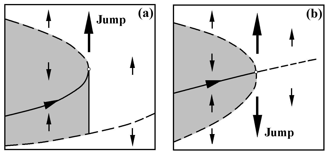
In the first picture, Figure 1(a), we illustrate both types of the saddle-node fold bifurcation: the static fold involving a path of equilibrium fixed-points, and the cyclic fold involving a trace of periodic orbits. For these the basin shrinkage is one-sided. The basin is bounded by the unstable side of the parabolically folding path.
Next, in Figure 1(b), we illustrate the local subcritical bifurcations of which the Hopf, flip and Neimark are codimension-one (we remember that the more familiar static pitchfork bifurcations are codimension-two, being structurally unstable against a symmetry-breaking perturbation). Here we see an unstable solution, which controls the basin boundary, shrinking parabolically around the stable solution, from which the (noise-free) system jumps out of our field of view as the control parameter, , reaches its critical value of .
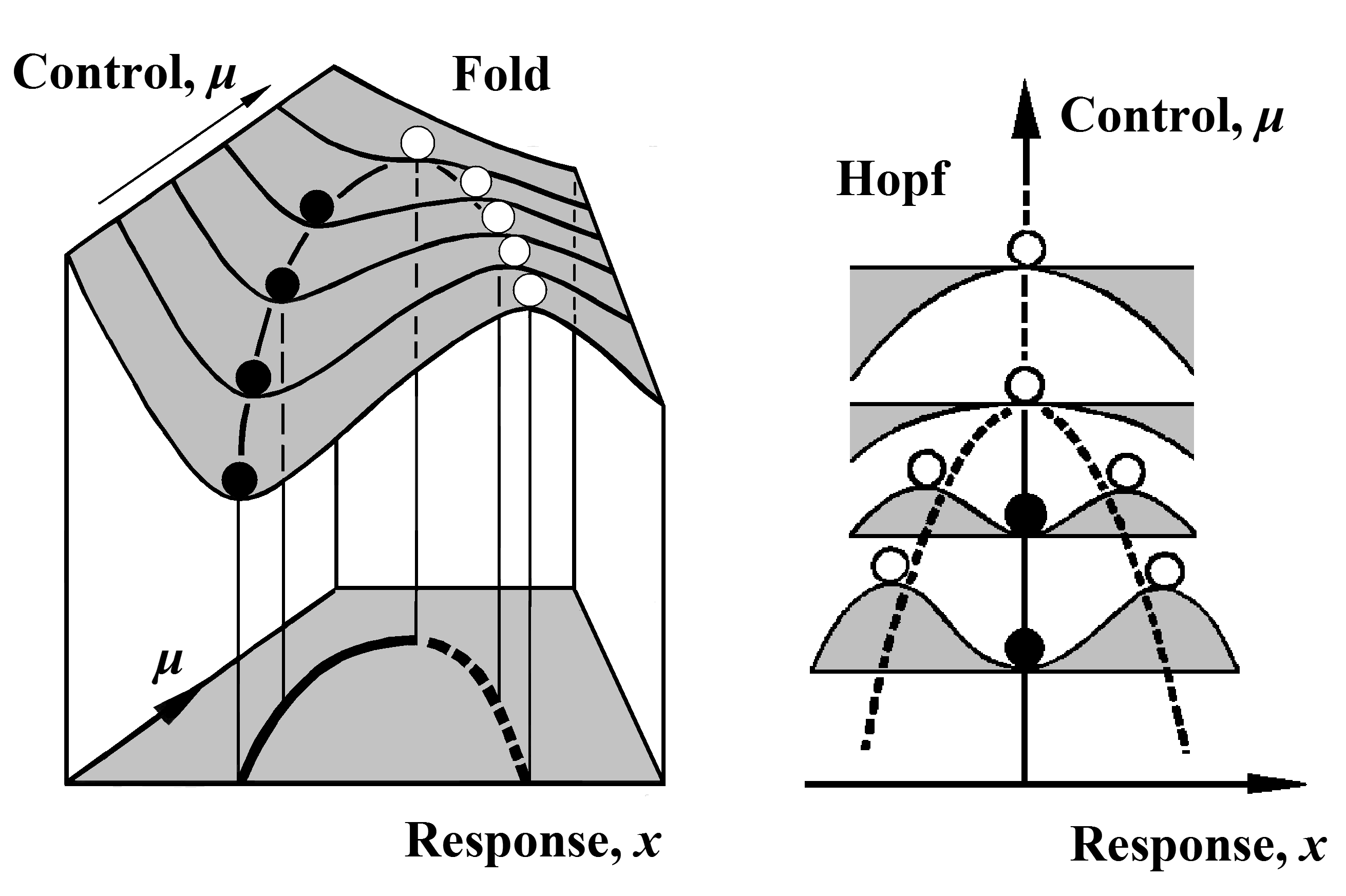
The static fold and the Hopf bifurcation have a theoretically well-defined potential energy surface that neatly summarizes the shrinking basin as illustrated in Figure 2. Note that Figure 2(a) will be discussed more fully in section 2(2.2).
2.2 A closer look at the fold
The fold is the simplest and most common way in which an equilibrium of a nonlinear dissipative dynamical system can lose its stability. Having only a single active degree of freedom () and being observable under the variation of a single control parameter () it can be illustrated on a graph of against as a smooth curve that simply reaches an extreme value (a maximum, say) of the control , as shown in Figure 1(a). So although it is traditionally called a saddle-node bifurcation, it does not exhibit any obvious ‘bifurcation’ of a path, but rather just a smooth folding of an existing path. In the case of a static fold (to which we shall largely restrict our attention) the path is a trace of equilibrium fixed points, while for a cyclic fold the path would be a trace of periodic solutions.
Assuming that we are close to a fold, the intrinsic damping of the system will have become super-critical so the system will have the non-oscillatory response of an over-damped particle sliding (in thick oil, as we might imagine) on a notional potential energy surface . This is illustrated for the fold in Figure 2(a), where we show the potential energy surface erected over the base plane. Here the solid part of the equilibrium path, corresponding to energy minima, is a stable node, while the dashed part, corresponding to energy maxima (more generally a geometrical saddle in higher dimensions) is an dynamically unstable saddle.
We see that as the control is slowly increased towards its critical value, , the stable equilibrium solution gets closer and closer to the hill-top potential barrier, and so gets progressively more precarious in the presence of noisy disturbances. With increasing at an infinitesimal rate, noise will ensure escape over the hill-top before reaches . If, however, increases rapidly, this early escape may be delayed or supressed as we have examined quantitatively elsewhere (Thompson and Sieber [12]).

To give a greater perspective to our view of the fold it is useful to introduce another control parameter such that our parameter space is now represented jointly by the -plane. We can now erect an equilibrium surface, of height , over the two-dimensional control plane as illustrated in Figure 3. Here we see two fold lines whose projections divide the control plane into regimes exhibiting either one or three co-existing solutions. These fold lines coalesce and vanish at the cusp. This cusp is a codimension-two phenomenon, which is typically only observed when we have independent control of both parameters ( and ). This is made transparent by the fact that a typical path in control space cannot be expected to pass precisely under the cusp point; by contrast, if a parameter path passes through a fold line all near-by paths also cross this fold line, which is what ‘the fold has codimension-one’ means. For an appropriate choice of path in the (-plane through the cusp one sees a pitchfork bifurcation (Thompson and Stewart [10]).
We will consider the case in which the main equilibrium sheet (in grey) is stable while the narrow inverted sheet (white) is unstable.
A climate system will have a large number of possible control parameters, but in trying to predict a tipping point we will be studying a particular evolution which corresponds to a particular route in control space; this is precisely why we are only likely to encounter a fold, and not a cusp in Figure 3. To explore possible scenarios that might underlie a tipping study, it is now useful to examine some possible routes in our two-parameter model of Figure 3.
Consider, first, the simple scenario in which the system parameters take path leading transversally through a fold line. This is the classical encounter with a fold that is implicitly envisaged in earlier work. In the presence of noise a premature tip from N occurs with a certain probability depending on the noise level and the speed with which the path is traversed, as analysed by Thompson and Sieber [11]. If the noise level were particularly high, a jump from N could easily be perceived as a purely noise-induced jump with no bifurcation, even though it is actually caused by the proximity to the fold: this could hold even if there were no movement in the control space at all, the system having rested at N throughout ([Ashwin et al. this volume] call this N-tipping). Another scenario, not specifically illustrated in the figure, could arise if the route in control space approached the fold line, but then turned back away from it. Analysis would then show a temporary decrease of the strength of the attraction (with the AR(1) coefficient moving towards unity) which might be discounted as a false alarm, even though the system did approach a fold and a noise-induced escape was temporarily probable.
Finally, in the scenario of path , one would observe a temporary increase of the AR(1) coefficient, even though no bifurcation is apparent but rather a gradual shift of the steady state. This shows that a rapid transition can be related to a nearby fold that was just barely missed. Similarly, the scenario called R-tipping by [Ashwin et al. this volume] occurs if one changes the other control parameter in Figure 3 sufficiently rapidly from the path to N (avoiding the folds). In this scenario the system jumps to the other stable equilibrium despite having never crossed a bifurcation curve.
3 Time series analysis for leading order terms — qualitative overview
The extraction of the underlying dynamics from time series is divided into subtasks of increasing difficulty. Assume that we have a time series coming from a process that is either stationary or has a slowly drifting underlying parameter as suggested by the paths in Figure 3. In order to predict (or identify) the dynamics one attempts to extract the leading orders of the dominant components of the underlying equations of motion.
We illustrate the steps using a time series obtained from a process which has the saddle-node normal form with a slowly drifting normal form parameter as its deterministic part (corresponding to Figure 2(a)) and is influenced by additive Gaussian noise. We permit the parameter to drift slowly with speed :
| (1) |
Here is the response, is the control parameter, and is the time. The Gaussian perturbation has zero mean and unit variance such that controls the noise induced variance added to the dynamics of the deterministic saddle-node form , which has the stable equilibrium . The second equation prescribes the linear sweep of from its starting value towards zero at rate . For fixed the unperturbed system () has a stable equilibrium at and an unstable equilibrium at .
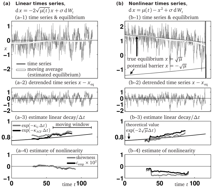
In Section 4 we will use the saddle-node normal form (1) to test the ability of a range of estimators to distinguish a time series generated by a process with a quadratic nonlinearity from a linear time series. Two example time series and their analysis are shown in Figure 4. Both time series have identical linear properties but differ in the dominant nonlinear term of the deterministic part of the dynamics.The softening of the full (estimated) nonlinear potential well (corresponding to the illustration in Figure 2(a)) is displayed in Figure 5.
3.1 Equilibrium — zero order
The location of the slowly drifting equilibrium and its trend is estimated first. [Lenton et al. this volume] call this step detrending and propose either piecewise linear fitting or filtering with a Gaussian kernel. The result of filtering with a Gaussian kernel is shown as a thick grey curve in the row 1 of Figure 4. Every method for detrending requires a bandwidth parameter (for example the width of the Gaussian kernel). For Figure 4 we chose the bandwidth which the kernel density estimation routine (Matlab’s kde by Botev et al. [14]) offered. The thin black curve in Figure 4(b-1) shows the true value of the quasi-equilibrium (for ). It gives a visual estimate of how the reliability of the zero-order estimates depends on the quality of the data. The oscillatory deviations of the extracted equilibrium (thick light grey curve) from its true value (thin black curve) shows that the automatically chosen bandwidth was slightly smaller than the theoretical optimum.
3.2 Linear decay rate — first order
Assuming that the deterministic part of the underlying process has a stable equilibrium (which is possibly slowly drifting), and that the zero-order estimate is an approximation for , the next step is to estimate the linear decay rate toward and the trend of over time. Generally, if the underlying deterministic process is high-dimensional then these estimates capture the dominant (that is, smallest) decay rate. They are typically applied to the detrended time series, that is, , which is shown in the second row of Figure 4.
-
•
ACF The -step (usually one-step) autocorrelation function (ACF) is fitted directly to the detrended time series: . This was introduced by Held and Kleinen [5] as degenerate finger-printing for the analysis of climate time series. The ACF is related to via
The estimate for is shown in Figure 4(a-3) and (b-3).
-
•
DFA Detrended fluctuation analysis has been introduced by Livina and Lenton [6] for climate time series, see also [Lenton et al. this volume] for a short description of how one extracts from this analysis.
-
•
Quasi-stationary density If one assumes that the deterministic dynamics of the detrended time series is essentially that of an overdamped particle moving in a potential well , that is,
(2) then the linear decay rate equals the second derivative of at the bottom of the well, . Moreover, the stationary density is related to the shape of the potential well via the stationary Fokker-Planck equation
(3) where is the constant of integration. This constant satisfies , and can be interpreted as the flow rate ( indicates flow toward ). Remembering that the drift speed of the system parameter is small, the true time-dependent probability density still satisfies (3) approximately at each :
(4) In (4) we included the dependence of all quantities on expressly and remember that is of order . Assuming quasi-stationarity, we neglect the order- terms and determine the coefficients, and , by fitting the empirical density from a time window to the Equation (4). Specifically, is a scalar and is equal to after detrending such that one has to fit two coefficients, and using (4) if one truncates after first order:
(5) In problems where no escape is possible one can drop the term in (3) (and, thus, in (4) and (5)), and simplify (3) to
(6) Livina et al. [15] used relation (6) (fitting of with higher-order polynomials) to detect potential wells in time series that included rapid transitions. Fitting with a parabola (where is irrelevant and ) is equivalent to using the variance of if the density is Gaussian. Ditlevsen and Johnsen [16] state that monitoring the empirical variance helps to avoid erroneous detection of false trends.
[Lenton et al. this volume] compare these three estimates, , the DFA-based estimate for , and the variance (which is inversely proportional to ), in detail using time series arising in climate models and in palaeoclimate records. Methods based on properties of the spectrum of the time series were proposed and investigated by Kleinen et al. [17], Biggs et al. [18] but are not discussed here. Figure 4 shows in row 3 how the estimates of from the quasi-stationary density compare to the ACF estimates . For both time series the estimates are quantitatively close to the theoretical value of (which is indicated by the thin black line in Figure 4(a-3,b-3)). We also observe that in Figure 4(a-3,b-3) the local trends of from the autocorrelation estimate and of based on the quasi-stationary density are strongly correlated, so it is unclear if monitoring both quantities really prevents false alarms.
There is one notable difference between the AR(1) and the DFA estimate on one hand and the distribution-based estimate on the other hand: the estimate for based on the quasi-stationary density only looks at the distribution of the values in the window of interest but does not care about the order in which they appear. This is in contrast to, for example, the AR(1) estimate which determines the correlation between each value and its predecessor.
Estimate of the input noise amplitude
If the AR analysis shows the presence of a single positive dominant coefficient (which gives evidence that the underlying dynamics has really one distinct direction in which the decay is slowest) then one can combine both estimates of the decay rate to obtain an estimate of the amplitude of the additive noise. Equations (3) and (5) imply that is an estimate for where and are the true linear decay rate and input noise amplitude. Thus, if we replace the unknown by the estimate we can use the relation between and the true to estimate :
| (7) |
where is the estimate of the linear decay rate obtained from the autocorrelation and is the estimate obtained from the quasi-stationary density . This is an alternative to using the residual of the least-squares fit that one obtains when estimating . We found that the residual systematically underestimates the noise level in the normal form examples shown in Fig. 4.
3.3 Nonlinearity — basin boundary
One problem left open by the linear analysis is that the quantitative value of the estimated linear decay rate and the estimated noise-level do not give any indication for the probability of tipping. What the linear methods estimate is the and the of a discrete process
| (8) |
(where the are assumed to be independent and normally distributed random numbers). The discrete process (8) is the linearisation of the time- map of the continuous process (2). An estimate for less than but close to unity does not necessarily indicate that we are close to a stability boundary for the nonlinear problem (2). Rather, it implies that the time step between successive measurements has been small compared to the mean decay time to half, , of the process:
The trend of the estimated is an indicator for incipient tipping because (if extrapolated in any way) it gives an estimate for the time to tipping if one ignores the possibility of early escape. However, the trend of is less certain even in the artificial time series of Figure 4. Similarly, the estimated noise amplitude has to be compared to the coefficient in front of the leading nonlinear term of the right-hand side (which equals in (1)). The ratio between and nonlinear term enters the estimates for the probability of tipping if there is no discernible upward trend in (N-tipping), or for the probability of early escape if the trend of points upwards (see Thompson and Sieber [12]). So without at least an order-of-magnitude estimate of the leading nonlinear term the linear methods only provide an estimate for the tipping time if there is a clearly discernible trend in , and even then this estimate discounts early escape.
Figure 4 illustrates this problem. Apart from a slow trend both time series in Figure 4 have identical properties at the linear level. However, while for the time series in Figure 4(b-1) the median time to tipping is according to Thompson and Sieber [12] (indeed, it escapes shortly after ), for the time series in Figure 4(a-1) the extrapolation (correctly) predicts tipping (or rather, linear instability) at . Thus, we observe that the linear properties of the time series alone are not sufficient to provide estimates about tipping, for example, the median time to tipping. The difference between the time series in Figure 4(a-1) and Figure 4(b-1) is in the dominant nonlinear term of the deterministic part. That this term plays a role is not surprising because tipping is a feature of nonlinear systems. Extracting its presence from a time series is a necessary step that has to follow the linear analysis.
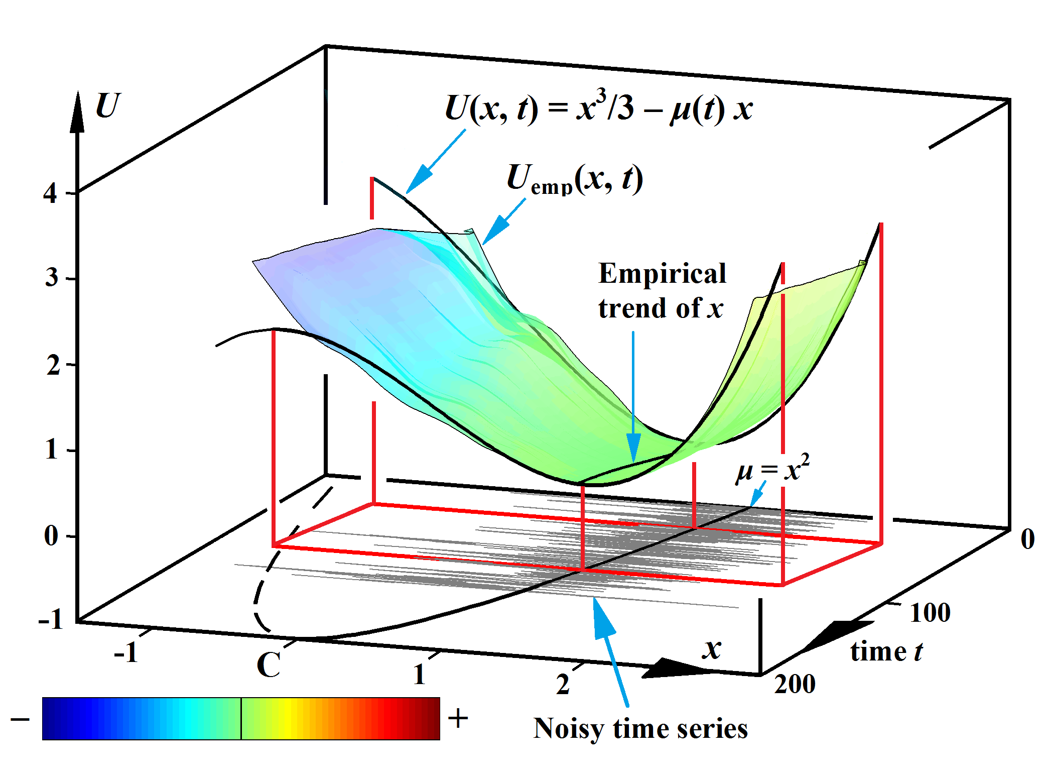
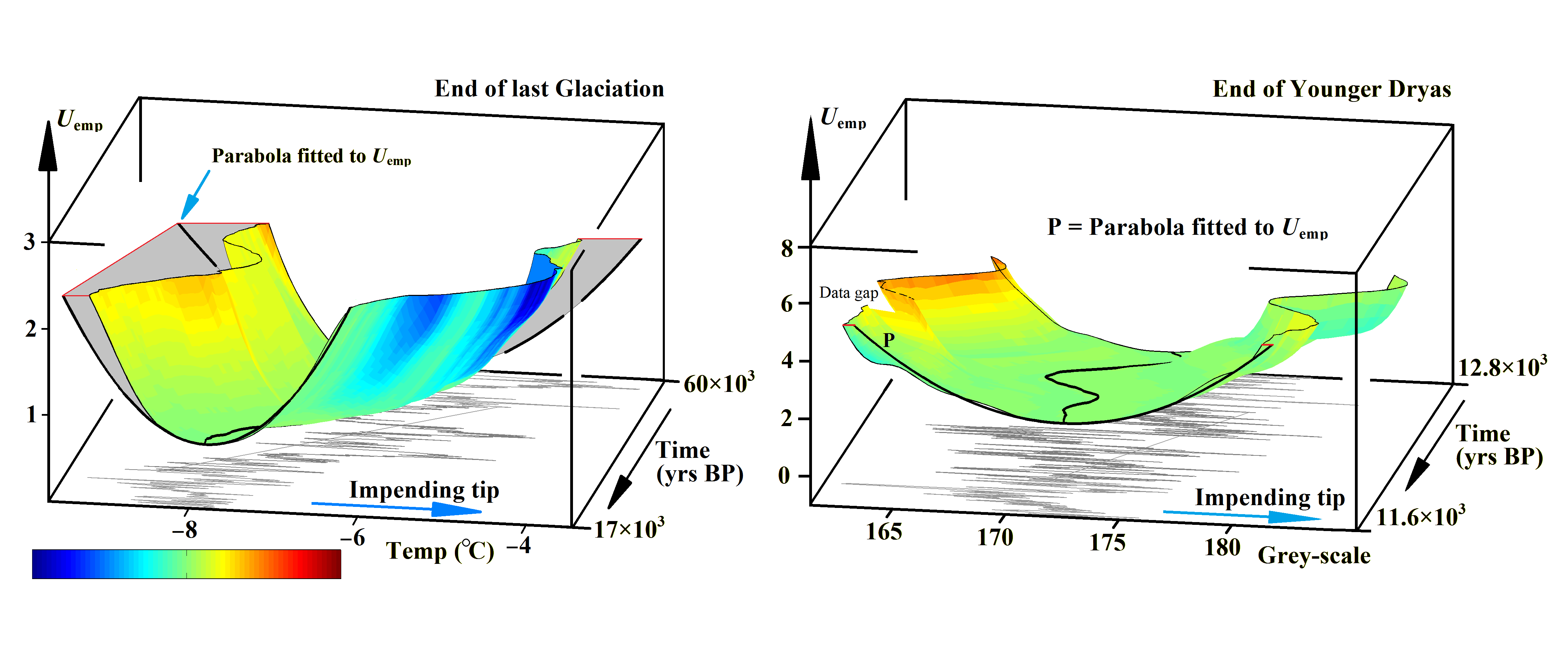
The approaches presented in the following all generalise the estimate for , based on the quasi-stationary density, by looking at the full nonlinear potential well associated to the quasi-stationary density via the Fokker-Planck equation (4). Figure 5 illustrates how looks like for the time series shown in Figure 4 column (b). The realisation of the noisy, evolving time series is shown in the base plane together with the equilibrium path , and the estimated (empirical) potential, is shown as the coloured surface. The estimate for the potential well is taken in a sliding window, which explains why the surface can only be determined in the central region of the time series with half the length of the window unrepresented at either end. The numerically estimated equilibrium trend is displayed as a black curve at the bottom of the valley of . For comparison with this we display at either end the real (nonlinear) potential corresponding to (1), which at the later time is already showing the hill-top to the left. The colour in Figure 5 shows the deviation of the empirical potential from the linear-theory parabola, which is not itself displayed. The softening, highlighted by the blue colouration, is seen on the left hand side which is approaching the hill-top. Transparency of the colour is used to show the number of data points that support a particular part of the surface (as given by the empirical quasi-stationary density ).
Several methods have been proposed to detect nonlinearity in the potential well in the form of this type of softening (or tilting).
-
•
Skewness Guttal and Jayaprakash [19, 20] studied how the closeness of a bifurcation influences the skewness of the empirical quasi-stationary density from time series. As this approach is also based on the empirical quasi-stationary density , it generalises the estimate to non-parabolic features of the well and non-Gaussian features of the stationary density. Guttal and Jayaprakash [19, 20] proposed to look at the trend of the skewness over time to detect incipient bifurcations. Figure 4(b-4) shows how the skewness, taken over a single window, changes. It is noticeably negative (compare to the empirical skewness from the linear time series in Fig 4(a-4)) but no trend is discernable.
-
•
Quasi-stationary density Livina et al. [15] generalised the potential well analysis for the quasi-stationary density beyond the estimate for the linear decay rate, fitting the potential well to higher-order polynomials of even degree using relation (6). This analysis was not used to attempt prediction of transition probabilities from time series but it was applied to time series that already included all transitions to count the number of wells of depending on time (which corresponds to the number of modes (peaks) of the empirical quasi-stationary density ). See also [Beaulieu et al. this volume] for methods that detect change points in time series.
-
•
Drift ratio If one assumes that the underlying system parameter is approaching a fold more or less linearly () and one is sufficiently close to the fold already then the ratio between the drift of the equilibrium estimate and the increase of the estimated linear decay rate estimates the quadratic term in the normal form [12].
4 Quantitative estimates of the nonlinear coefficients
The colour shading of Figure 5 suggests that the nonlinear term in the underlying deterministic system shows up in the quasi-stationary density . This raises two questions. First, can the level of deviation from linear theory be distinguished with confidence from random chance? That is, can one state, when looking at a time series, that a significant quadratic term is present? Second, is it possible to quantify the size of the nonlinear term with reasonable level of certainty?
Finding a significant nonlinearity is far easier than estimating its precise value because biases introduced during the analysis of the equilibrium and decay rate (zero-order and first-order analysis) may distort the value of the nonlinear estimate but may still keep it significantly different from zero. We will demonstrate this in Section 5 for two paleo-climate time series.
4.1 Properties of the stationary density of the saddle-node normal form
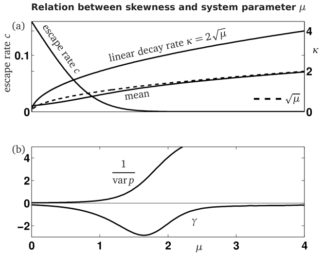
Figure 6 shows the dependence of the mean, the variance , and the skewness of the empirical stationary density on the system parameter for (1) as computed using the stationary Fokker-Planck equation (3). Note that this corresponds to the stationary process where the random realisation is re-injected at whenever it has escaped to . We observe that the dependence of is strongly nonlinear for the saddle-node normal form with noise (, in Equation (1)). This means that trends of the skewness are likely to be difficult to ascertain when approaching a fold. However, the presence of skewness is an indicator for the nonlinearity uniformly for all parameters , and its sign indicates the direction of escape.
Note also how the nonlinearity affects the empirical mean and the variance , which is no longer inversely proportional to the linear decay rate . This shift of the mean and the additional variance is in part due to the fraction of trajectories that escape, in part due to the non-parabolic shape of the well at some distance from its local minimum.
4.2 Practical estimates of the nonlinear term from time series
We can estimate the nonlinearity directly as the deviation of the empirical potential well from a parabola as suggested by figure 5 (we are only interested in ). The simplest approach (apart from looking at skewness ) is to fit and to the empirical density using Equation (5). If is indeed linear then would be zero such that is a signed scalar measure for the deviation of from linearity, serving as a proxy for the present nonlinearity. A second alternative is to expand to second order, incorporating a quadratic nonlinearity directly into with an unknown coefficient . This leads to
| (9) |
Both quantities, and , measure the deviation of from its linear approximation . The main difference between them is the weighting ( for , uniform for ). In summary, the step-by-step procedure to extract an estimate of the quadratic term (or a proxy for it) from a time series is the following.
- 1.
-
2.
Choose a length of sliding windows and obtain the empirical stationary density for the sliding window centered at . (We used kde1d to obtain . For non-stationary time series we used the sliding window length .)
- 3.
4.3 Comparison of estimates using saddle-node normal form
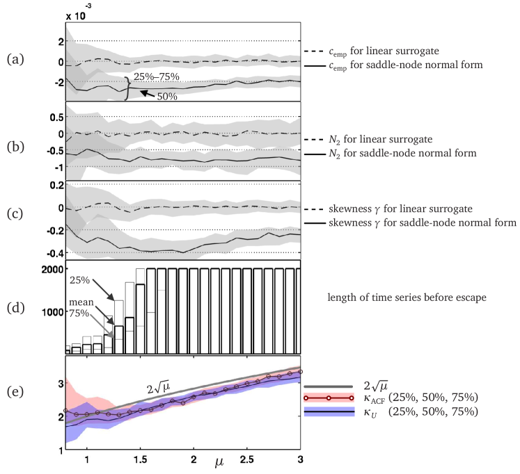
Figure 7 shows how the estimates for nonlinearity behave for the saddle-node normal form with noise, Equation (1) with and . Each panel shows the quartiles of the distribution of the estimate for realisatons of time series generated by (1). Each realisation was run until it reached data points or (indicating escape). Panel (a) shows the estimate obtained by linear-least-squares fitting of the approximate stationary Fokker-Planck equation (5) to the empirical stationary density , panel (b) shows the quadratic coefficient obtained from (9), and panel (c) shows the skewness of . For comparison, we generate also linear time series using
| (10) |
and then fit , and for these time series, too. Figure 7 compares the quartiles of the distributions for time series generated by the saddle-node normal form (1) and the linear equation (10). If there is small overlap in the distribution then the quantity is a good indicator for the presence of a quadratic nonlinear term. We observe that this is the case for all quanitites as long as the time series has a length of (see Figure 7(d) for the distribution of time series lengths). Naturally, the uncertainty, and, hence, the overlap, increases when the time series is shorter due to escape from the potential well to . This is the case for smaller in Figure 7 (see Thompson and Sieber [12] for a quantitative study of escape probabilities for small ). We also notice that all quantities have a systematic deviation from the theoretical value of the quantity they supposedly estimate: should be equal to according to (1), the real escape rate has a much smaller modulus than (compare Figure 6(a)), and the skewness has theoretically a much larger modulus (compare Figure 6(b)). The deviation for is relatively small, and is likely caused by the kernel density estimate for . The large modulus of shows that the linear term is a poor fit for , which makes a measure of how much the odd symmetry is broken by , rather than an estimate for the escape rate. We note that as fitted in (9) has a realistic modulus (close to zero, not shown in Figure 7). The bias of the skewness is mainly due to our restriction to time series that stay inside the potential well. However, the characteristic dip of seen in Figure 6(b) is still visible in Figure 7(c). 10 addresses the dependence of the empirical skewness on all method parameters.
We also note that the estimates for the linear decay rate, and are more accurate than the the estimates for the nonlinearity but by their nature they cannot distinguish the time series generated by the saddle-node normal form from a linear surrogate.
The summative conclusion from Figure 7 is that one can detect the underlying nonlinearity of the deterministic part of Equation (1) by observing , or the skewness if the time series is moderately long. One can expect this to be true in the more general case of a time series generated by a system with deterministic dynamics close to a fold and additive noise. While one can in principle recover the underlying parameter from the estimates for , and (see Thompson and Sieber [12]), the uncertainty in propagates dramatically into uncertainty for (one has to divide by ).
The results of Figure 7 show the stationary case (). For slowly drifting time series the same analysis will then have to be applied to parts of the time series in sliding windows. We demonstrate this for two geological times series in Section 5. For time series with rapidly drifting system parameter the estimates for the softening, , and the skewness , will not give a detectable difference from the corresponding linear time series before tipping. The conclusion one would draw from this absence of detectable softening would be correct: tipping happens when the linear decay rate reaches the critical value (or slightly later, see Thompson and Sieber [12]). The same holds if the noise level is low, which is equivalent to rapid drift (see Thompson and Sieber [12] for the transformation). In practice one uses the argument the other way round: if the nonlinear estimates do not give a value significantly different from zero one will conclude that the ratio between noise level and drifting speed is small.
5 Studies of Geological Time Series
We now apply our nonlinear investigations to two ancient climate tippings. The first is the major transition marking the end of the latest ice age which occurred about years before the present (yrs BP). The data used for this is a temperature reconstruction from the Vostok ice core deuterium record (Petit et al. [22]). The second more recent tipping is the ending of the Younger Dryas using the grayscale from the Cariaco basin sediments in Venezuela (Hughen [23]). This Younger Dryas event was a curious cooling, about years ago, just as the Earth was warming up after the last ice age. It ended in a dramatic tipping point, when the Arctic warmed by in years. This sudden ending has been related (Houghton [24]) to a switching-on of the global oceanic thermohaline circulation (THC). This switch-on is known from extensive theoretical studies (Dijkstra and Weijer [25]) to be at a saddle-node fold arising as a perturbation of a sub-critical pitchfork (see, for example, Rahmstorf [26] and Thompson and Sieber [12]).
Under linear time-series analysis of the directly preceding data, neither of these two events shows a strong trend in the stability propagator (see Figure 9). Meanwhile sample estimates of the underlying potential functions are shown in Figure 8.
In Figure 8(a), for the end of the last glaciation, we see clearly that the well is softening (falling beneath the parabolic fit) on the high-temperature end while hardening (rising above the parabola) on the low-temperature end. So there is a strong nonlinear signal that a jump to higher temperatures may be pending (as indeed it was). We show that this signal is statistically significant in our full analysis in Figure 9. By comparison, the study of the Younger Dryas, illustrated in Figure 8(b), provided no significant nonlinear conclusions.
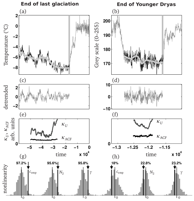
For Figure 9 we detrended both time series using Gaussian filtering (see Figures 9(c) and (d)) and estimated the linear indicators and . We observe weak to non-existent trends, leaving the evidence inconclusive at the linear level (grey and black curves Figure 9(e) and (f)). The ratio between and , both shown in Figure 9(e) and (f), gives an estimate of the variance of the noise input. The unit for is units of per time step (so, for example for Fig. 9 (e) ), and, correspondingly, the unit for is (unit of divided by unit for ). Both units are arbitrary such that we do not indicate the scale of the -axis in Figure 9(e,f).
[Lenton et al. this volume] discuss the linear analysis of both time series in greater detail. Their time series Vostok corresponds to Figure 9(a), their time series Cariaco corresponds to Figure 9(b). (Note that [Lenton et al. this volume] use the deuterium proxy directly whereas Figure 9(a) shows the temperature reconstruction.) Specifically, Figures 2 and 4, and Figures 9 and A1 in [Lenton et al. this volume] discuss how the results depend on method parameters such as detrending bandwidth and sliding window. Their analysis finds that the presence of a significant trend depends strongly on both parameters. See [Lenton et al. this volume] , Table 1 (rows Vostok and Cariaco), for a summary of the evidence at the linear level.
At the nonlinear level, the time series for the end of the last glaciation has a strong quadratic nonlinearity in where the potential well is presumed to govern the deterministic part of the dynamics (Figure 9(g)). The indicators , and the skewness in Figure 9(g) are all far removed from what can be expected by chance in a linear time series. The histogram in the background of Figure 9(g,h) has been sampled from random linear time series generated by the linear process given in Equation (10) with where is taken from the estimate shown in Figure 9(e). The percentages at the top of Figure 9(g,h) express how far in the tail of the histogram the mean of the quantity extracted from the geological time series is. We warn that the three quantities , and are not really three independent indicators as they all depend on the same estimate of the empirical density .
Visual inspection of the well shape in Figure 8 confirms that the well is softening (bending downward) on the high-temperature end and hardening (bending upward) on the low-temperature end. So, at the nonlinear level the time series data close to the bottom of the well gives already evidence for a propensity to escape toward larger temperatures. The time series for the end of the Younger Dryas does not show evidence for strong nonlinearity of the underlying dynamics at the second-order level (Figure 9(h)). The values for , and the skewness can all be explained by randomness as the histograms of estimates for the linear time series (as the histograms in Figure 9(h) show). Note that we did not include the previous transition (visible at the left end in Figure 9(b)) into our analysis as our aim was to infer the nonlinearity exclusively from the data near the tipping equilibrium.
6 Conclusion
The main message of the paper is that the linear analysis investigated by [Lenton et al. this volume] on its own, even if all estimates are accurate, does not contain all information necessary to estimate the probability of tipping over time. The result of the linear analysis is an estimate of the decay rate , which is taken relative to the time spacing of the measurements. Even if this decay rate has an identifiable trend to zero the probability of tipping over time is determined by the dominant nonlinear coefficient in conjunction with and the noise level.
We found that the dominant nonlinear coefficient is much harder to estimate accurately, so we also looked at proxies that indicate nonlinearity such as the skewness (as proposed by Guttal and Jayaprakash [19]) or the coefficient from Equation (5) (which is also a scalar signed measure for deviation from linear theory). Our study of the saddle-node normal form suggests that both proxies, and , give values that are easier to distinguish from random chance than the estimate for itself. A significantly non-zero value of either of these proxies indicates that a quadratic nonlinear term is present and gives its sign.
However, we found the uncertainty for moderately long time series () too large to translate the proxy back into a quantitatively reliable estimate for the normal form parameter (this would be necessary to read off the probability for tipping from the tables in Thompson and Sieber [12]). We also found that the nonlinear proxies do not have discernible trends when one approaches tipping, so it makes sense only to extract their overall mean from the time series but not the trend.
References
- IPCC [2007] IPCC. 2007 Climate Change 2007, Contribution of Working Groups I-III to the Fourth Assessment Report of the Intergovernmental Panel on Climate Change, I The Physical Science Basis, II Impacts, Adaptation and Vulnerability, III Mitigation of Climate Change. Cambridge: Cambridge University Press.
- Lenton et al. [2008] Lenton, T. M., Held, H., Kriegler, E., Hall J. W., Lucht, W., Rahmstorf, S. & Schellnhuber, H.-J. 2008 Tipping elements in the Earth’s climate system. Proceedings of the National Academy of Sciences of the United States of America, 105(6), 1786–1793.
- Scheffer [2009] Scheffer, M. 2009 Critical Transitions in Nature and Society. Princeton: Princeton University Press.
- Launder and Thompson [2010] Launder, B. & Thompson, J. M. T. editors 2010 Geo-Engineering Climate Change: Environmental necessity or Pandora’s Box? Cambridge: Cambridge University Press.
- Held and Kleinen [2004] Held H. & Kleinen, T. 2004 Detection of climate system bifurcations by degenerate fingerprinting. Geophysical Research Letters, 31(23), L23207.
- Livina and Lenton [2007] Livina, V. N. & Lenton, T. M. 2007 A modified method for detecting incipient bifurcations in a dynamical system. Geophysical Research Letters, 34(3), L03712.
- Dakos et al. [2008] Dakos, V., Scheffer, M., van Nes, E. H., Brovkin, V., Petoukhov, V., Held, H. 2008 Slowing down as an early warning signal for abrupt climate change. Proceedings of the National Academy of Sciences of the United States of America, 105(38), 14308–14312.
- Lenton et al. [2011] Lenton, T. M., Livina, V. N., Dakos, V., van Nes, E. H. & Scheffer, M. 2011 Early warning of climate tipping points : comparing methods to improve robustness. Phil. Trans. Roy. Soc. A, this volume.
- Thompson et al. [1994] Thompson, J. M. T., Stewart, H. B. & Ueda, Y. 1994 Safe, explosive, and dangerous bifurcations in dissipative dynamical systems. Physical Review E, 49(2), 1019–1027.
- Thompson and Stewart [2002] Thompson J. M. T. & Stewart, H. B. 2002 Nonlinear dynamics and chaos, 2nd edn. Chichester: Wiley.
- Thompson and Sieber [2010] Thompson, J. M. T. & Sieber, J. 2010 Predicting Climate Tipping Points. In Geo-Engineering Climate Change: Environmental necessity or Pandora’s Box?, chapter 3, pp 50–83, Cambridge: Cambridge University Press.
- Thompson and Sieber [2011] Thompson, J. M. T. & Sieber, J. 2011 Climate tipping as a noisy bifurcation: a predictive technique. IMA Journal of Applied Mathematics, 76(1), 27–46.
- Ashwin et al. [2011] Ashwin, P., Wieczorek, S., Vitolo, R. & Cox, P. 2011 Tipping points in open systems: bifurcation, noise-induced and rate-dependent examples in the climate system. Phil. Trans. Roy. Soc. A, this volume.
- Botev et al. [2010] Botev, Z. I., Grotowski, J. F. &Kroese, D. P. 2010 Kernel density estimation via diffusion. The Annals of Statistics, 38(5), 2916–2957.
- Livina et al. [2011] Livina, V. N., Kwasniok, F., Lohmann, G., Kantelhardt, J. & Lenton, T. M. 2011 Changing climate states and stability: from pliocene to present. Climate Dynamics, 37, 2437–2453.
- Ditlevsen and Johnsen [2010] Ditlevsen, P. D. & Johnsen, S. J. 2010 Tipping points: Early warning and wishful thinking. Geophysical Research Letters, 37(19), L19703.
- Kleinen et al. [2003] Kleinen, T., Held, H. & Petschel-Held, G. 2003 The potential role of spectral properties in detecting thresholds in the Earth system: application to the thermohaline circulation. Ocean Dynamics, 53(2), 53–63.
- Biggs et al. [2009] Biggs, R., Carpenter, S. R. & Brock, W. A. 2009 Turning back from the brink: detecting an impending regime shift in time to avert it. Proceedings of the National Academy of Sciences of the United States of America, 106(3), 826–831.
- Guttal and Jayaprakash [2008a] Guttal, V. & Jayaprakash, C. 2008a Changing skewness: an early warning signal of regime shifts in ecosystems. Ecology Letters, 11(5), 450–60.
- Guttal and Jayaprakash [2008b] Guttal, V. & Jayaprakash, C. 2008b Spatial variance and spatial skewness: leading indicators of regime shifts in spatial ecological systems. Theoretical Ecology, 2(1), 3–12.
- Beaulieu et al. [2011] Beaulieu, C., Chen, J. &Sarmiento, J. L. 2011 Change point analysis as a tool to describe past climate variations. Phil. Trans. Roy. Soc. A, this volume.
- Petit et al. [1999] Petit, J. R., Jouzel, J, Raynaud, D., Barkov, N. I., Barnola, J.-M., Basile, I., Bender, M., Chappellaz, J., Davis, M., Delaygue, G., Delmotte, M., Kotlyakov, V. M., Legrand, M., Lipenkov, V. Y., Lorius, C., Pépin, L., Ritz, C., Saltzman, E. & Stievenard, M. 1999 Climate and atmospheric history of the past 420,000 years from the Vostok ice core, Antarctica. Nature, 399(6735), 429–436.
- Hughen [2000] Hughen, K. A. 2000 Synchronous Radiocarbon and Climate Shifts During the Last Deglaciation. Science, 290(5498), 1951–1954.
- Houghton [2004] Houghton, J. T. 2004 Global warming: the complete briefing. Cambridge: Cambridge University Press, Cambridge.
- Dijkstra and Weijer [2005] Dijkstra, H. A. & Weijer, W. 2005 Stability of the global ocean circulation : Basic bifurcation diagrams. Journal of Physical Oceanography, 35(6), 933–948.
- Rahmstorf [2000] Rahmstorf, S. 2000 The Thermohaline Ocean Circulation: A System with Dangerous Thresholds? Climatic Change, 46(3), 247–256.
Sensitivity analysis for estimates of nonlinear quantities in palaeoclimate records Figure 10 shows how the results in Figure 9(g,h) depend on our method parameters. Specifically, we vary the length of the sliding window and the bandwidth of the Gaussian kernel when fitting the quasi-equilibrium drift.
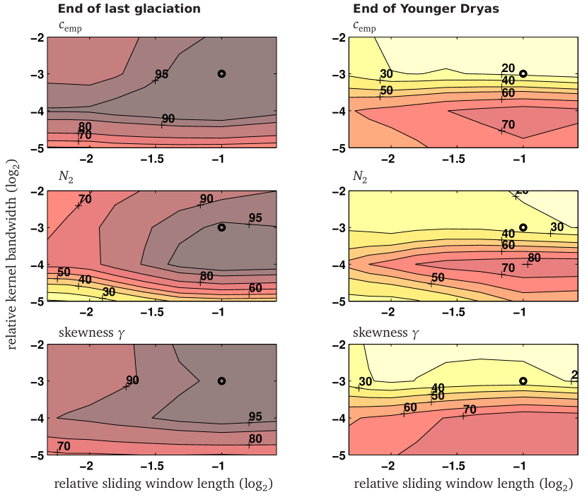
In all panels the -axis is the length of the sliding window relative to the overall length of the time series on a logarithmic scale (overall length is for the end of the last glaciation, for the end of the Younger Dryas). For example, the -value of corresponds to a window length . The -axis is the kernel bandwidth for the Gaussian fitting kernel relative to the overall length of the time series on a logarithmic scale (this enters the function kde1d as a resolution parameter). For example, the -value of means that the resolution parameter of kde1d is .
For each measured quantity we compare the mean of its value over all sliding windows to the percentiles of the linear surrogate. In this way contour levels close to or correspond to significant deviations from a time series generated by a linear process. The distributions of these time series are shown as gray background in Fig. 9(g,h). The value shown as a black vertical line in Figure 9(g,h) was obtained using the method parameters highlighted by a black circle in Figure 10.
Fig. 10 gives evidence that the nonlinear features of the time series for the end of the last glaciation are robust as long as the detrending remains coarse grained. The end of the Younger Dryas does not show any nonlinear feature that is significantly different from the surrogates for any choise of method parameters. Dependence of skewness on distance to tipping point The observations in Figure 6(b) and Figure 7(c) appear to contradict the statement by Guttal and Jayaprakash [19] that skewness increases as one approaches tipping. Furthermore, there is a quantiative difference between Figure 6(b) and Figure 7(c), even though they show the same qualitative feature: non-monotonicity of the skewness in the control parameter . Note that Guttal and Jayaprakash [19] studied the same type of tipping as Figure 6, however, not in the fold normal form but in a particular ecological model. In order to investigate this apparent contradiction we look at how the skewness depends on two parameters: the control parameter and the value at which we consider a realisation as escaped. More precisely, both figures, 6(b) and 7(c), study
| (11) |
where without loss of generality and is constant. Any realisation of (11) escapes to in finite time almost surely such that (11) does not possess a stationary density. In the calculation for Figure 6 we modified the process (11) by re-injecting the realisation at whenever it escaped to . In this way the process has a stationary density given by the Fokker-Planck equation (3) with . However, this is not accurately describing the density that one is interested in: the probability density of the realisations under the condition that the realisation has not yet ‘escaped’. Clearly, this conditional probability depends on what one means by escaped. So, we introduce the escape boundary as an additional parameter. Whenever, a realisation gets smaller than the value (that is, it has run away beyond the local maximum of the potential by distance ) we stop the integration of (11). When one considers the set of all realisations before escape then this also leads to a stationary density. This was done for Figure 7 using (such that we count a realisation as escaped whenever it reaches ). The re-injection used for Figure 6 and the choice of as escape indicator lead to the systematic difference in skewness between the figures 7(c) and 6(b). In practice one encounters only the conditional probability as shown in Figure 7. So, it is important to check how the skewness depends on the somewhat arbitrary choice of the the value indicating escape. Moreover, the estimate shown in Figure 7(c) suffers from the shorteness of the time series for close to (which is typical in practice).
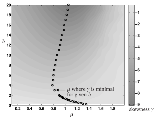
Figure 11 shows the result of a more precise calculation: we simulate (11) for a large ensemble of realisations (). At every time step we collect the realisations that have reached a value . They count as escaped and have to be discarded. In order to avoid depletion of the ensemble we start new realisations at . For each newly started realisation we pick the current value of one randomly chosen non-escaped realisation as the inital value. This process reaches a stationary density, which is an approximation of the conditional probability density of under the condition that has not yet escaped beyond . We observe in Figure 11 that the depth of the dip in the skewness depends on (indicated by grayscale) but that the location of the dip is uniformly larger than the critical value of the control parameter .
It is possible that the simulations by Guttal and Jayaprakash [19] stayed consistently to the right of the curve of extreme skewness shown in Figure 11 such that only the increase is observed. Note that in their model the notion of skewness has the opposite sign, so one should consider the modulus of the skewness.