Many-Body Contributions to Green’s Functions and Casimir Energies

Abstract

The multiple scattering formalism is used to extract irreducible $N$-body parts of Green’s functions and Casimir energies describing the interaction of $N$ objects that are not necessarily mutually disjoint. The irreducible $N$-body scattering matrix is expressed in terms of single-body transition matrices. The irreducible $N$-body Casimir energy is the trace of the corresponding irreducible $N$-body part of the Green’s function. This formalism requires the solution of a set of linear integral equations. The irreducible three-body Green’s function and the corresponding Casimir energy of a massless scalar field interacting with potentials are obtained and evaluated for three parallel semitransparent plates. When Dirichlet boundary conditions are imposed on a plate the Green’s function and Casimir energy decouple into contributions from two disjoint regions. We also consider weakly interacting triangular–and parabolic-wedges placed atop a Dirichlet plate. The irreducible three-body Casimir energy of a triangular–and parabolic-wedge is minimal when the shorter side of the wedge is perpendicular to the Dirichlet plate. The irreducible three-body contribution to the vacuum energy is finite and positive in all the cases studied.

I Introduction

The total energy $E_{12}$ of two static disjoint objects may be decomposed as,

$$E_{12}=E_{0}+\Delta E_{1}+\Delta E_{2}+\Delta E_{12},$$ (1)

where $E_{0}$ is the energy of the vacuum (medium) without objects, $\Delta E_{1}$ and $\Delta E_{2}$ are (self)-energies required to create the objects individually in isolation, and $\Delta E_{12}$ is the change in energy due to their interaction. The interaction energy $\Delta E_{12}$ is finite for disjoint objects if it is mediated by an otherwise free quantum field whose interaction with the objects is described by local potentials. It is the only contribution to the total energy that depends on the position and orientation of both objects and determines the forces between them. Casimir found that the electromagnetic force between two parallel neutral metallic plates does not vanish Casimir:1948dh and that the associated Casimir energy $\Delta E_{12}$ may be interpreted as arising from changes in the zero-point energy due to boundary conditions imposed on the electromagnetic field by the metallic plates. Zero-point energy contributions to the energies $\Delta E_{i}$ of individual objects in general diverge but the change $\Delta E_{12}$ due to the presence of two disjoint objects is finite.

Reliable extraction of finite Casimir energies for a long time appeared to be restricted to very special geometries, like parallelepipeds Lukosz:1971 ; Ambjorn:1981xw ; Ambjorn:1981xv , spheres Boyer:1968uf ; Milton:1978sf , and cylinders DeRaad1981229 . A multiple scattering formulation for computing Casimir energies of smooth objects was developed by Balian and Duplantier Balian1977300 ; Balian1978165 but it relied heavily on idealized boundary conditions. Kenneth and Klich only recently observed Kenneth:2006vr that $\Delta E_{12}$ may be computed independent of single-body contributions to the energy and is always finite for disjoint objects. This two-body interaction energy is compactly expressed Kenneth:2006vr ; Emig:2007me in terms of the free Green’s function, $G_{0}$, and transition operators, $T_{1}$, $T_{2}$, associated with the individual objects,

$$\Delta E_{12}=\frac{1}{2}\int_{-\infty}^{\infty}\frac{d\zeta}{2\pi}\,\text{Tr}\ln\big{[}1-G_{0}T_{1}G_{0}T_{2}\big{]}=\frac{1}{2}\int_{-\infty}^{\infty}\frac{d\zeta}{2\pi}\,\text{Tr}\ln\big{[}1-\tilde{T}_{1}\tilde{T}_{2}\big{]},$$ (2)

where we have defined partly amputed transition operators $\tilde{T}_{i}=G_{0}T_{i}$, $i=1,2$. For potential scattering the interaction energy may equivalently be expressed Milton:2007wz in terms of the potentials $V_{i}$ and the corresponding Green’s functions $G_{i}$ satisfying $G_{i}V_{i}=G_{0}T_{i}$.

In deriving Eq. (2) one formally subtracts divergent self-energies and avoids the question of whether these divergences have any physical significance. One in particular circumvents the issue raised in Brown:1969na ; Deutsch:1978sc of how they should be treated in the context of gravity, a problem that has so far only been considered for parallel plates Fulling:2007xa ; Milton:2007ar ; Shajesh:2007sc . Although it does not address such conceptual points, the irreducible contribution of Eq. (2) suffices to explain experimental measurements of Casimir forces between two disjoint objects. Since the interaction energy for disjoint objects is finite, errors due to numerical or other approximations to Eq. (2) can be controlled. This has now been demonstrated by explicit calculations for a number of geometries and physical situations CaveroPelaez:2008tj ; CaveroPelaez:2008tk ; Maghrebi:2010wp ; Maghrebi:2010jx .

In this article we examine a recently proposed extension of these ideas to more than two bodies. It was shown in Schaden:2010wv that the irreducible $N$-body part of the total energy remains finite if the $N$ objects have no common intersection. We here explicitly evaluate the irreducible three-body part, $\Delta E_{123}$, of the total energy,

$$E_{123}=E_{0}+\Delta E_{1}+\Delta E_{2}+\Delta E_{3}+\Delta E_{12}+\Delta E_{23}+\Delta E_{31}+\Delta E_{123},$$ (3)

in several cases and verify that $\Delta E_{123}$ remains finite even as irreducible two-body contributions diverge. The formal expression for $\Delta E_{123}$ given in Schaden:2010wv is considerably more involved than Eq.(2),

$$\Delta E_{123}=\frac{1}{2}\int_{-\infty}^{\infty}\frac{d\zeta}{2\pi}\,\text{Tr}\ln\Big{[}1+X_{12}\Big{\{}\tilde{T}_{1}\tilde{T}_{2}\tilde{T}_{3}X_{23}+\tilde{T}_{1}\tilde{T}_{3}\tilde{T}_{2}X_{32}-\tilde{T}_{1}\tilde{T}_{2}\tilde{T}_{1}\tilde{T}_{3}-\tilde{T}_{1}\tilde{T}_{3}\tilde{T}_{2}\tilde{T}_{3}X_{23}-\tilde{T}_{1}\tilde{T}_{2}\tilde{T}_{3}\tilde{T}_{2}X_{32}\Big{\}}X_{13}\Big{]},$$ (4)

where the $X_{ij}$’s are solutions to the integral equations,

$$\big{[}1-\tilde{T}_{i}\tilde{T}_{j}\big{]}X_{ij}=1.$$ (5)

We here obtain and evaluate alternate expressions for irreducible Casimir energies that do not involve a logarithm. The article is organized as follows. In Section II we derive Faddeev-like equations for the scattering matrix associated with $N$-objects and extract their irreducible $N$-body parts. The associated $N$-body Green’s functions are expressed in terms of one-body transition matrices describing scattering off each object individually. The procedure is illustrated for $N=2$, and $N=3$, for which explicit solutions are obtained. The method is generalizable to higher $N$. The general solutions of Section II are used to obtain the Green’s functions for two and three semitransparent plates in Section III. The irreducible three-body contribution to the Green’s function for three semitransparent plates is found to exactly cancel the two-body interaction of the outer plates when Dirichlet boundary conditions are imposed on the central plate.

In Section IV we express the irreducible $N$-body contribution to the Casimir energy in terms of the $N$-body part of the transition matrix. This avoids the computation of the logarithm of an integral operator, but requires one to solve a set of linear Faddeev-like integral equations for the $N$-body transition matrix. In Section V we use this formalism to obtain irreducible two–and three-body contributions to the Casimir energy of two and three semitransparent plates. The three-body contribution again cancels the two-body interaction from the outer plates when Dirichlet boundary conditions are imposed on the central plate.

In Section VI, we specialize to the case when two of the three potentials are weak. For point-potentials we prove that the irreducible two-body Casimir energy is always negative whereas the irreducible three-body contribution is positive. The proof immediately generalizes to any form of the weakly interacting potentials. We also derive expressions for irreducible two–and three-body contributions to the Casimir energy when the weak potentials have translational symmetry and the third potential represents a Dirichlet plate parallel to the symmetry axis. Some of the expressions for the irreducible two-body contributions appear to not have been noted in earlier studies. We obtain the irreducible three-body contribution to the Casimir energy in this semiweak approximation, and verify independently that it is positive and finite.

In Section VII we use these results to investigate the irreducible three-body Casimir energy of a weakly interacting wedge placed atop a Dirichlet plate forming a waveguide of triangular cross-section. The potentials forming the triangular waveguide overlap and the irreducible two-body contributions to the vacuum energy diverge. However, the irreducible three-body Casimir energy is well defined as long as the supports of the three potentials have no common overlap. The irreducible three-body Casimir energy is minimal (and vanishes) when the shorter side of the wedge is perpendicular to the Dirichlet plate. Inspired by the study in Abalo:2010ah , we investigate the dependence of the irreducible three-body Casimir energy on the cross-sectional area and perimeter of the triangular waveguide. To emphasize that the finiteness of the irreducible three-body Casimir energies is not only due to the subtraction of corner divergences, we, in Section VIII, consider a waveguide with weakly interacting sides of parabolic cross-section that touch a Dirichlet plate. The conclusions for weak triangular-wedges generalize to parabolic-wedges with only minor changes in interpretation.

The explicit calculations in this article support the general results of Schaden:2010wv . The irreducible three-body contribution to the Casimir energy in the examples considered here is always positive. It furthermore is continuous (and in this sense is analytic in the corresponding parameter) when two of the bodies approach each other and intersect.

II Many-body Green’s functions

The free Green’s function of a massless scalar field in Euclidean space-time satisfies the partial differential equation

$$[-{\bm{\nabla}}^{2}+\zeta^{2}]G_{0}({\bf x},{\bf x}^{\prime})=\delta^{(3)}({\bf x}-{\bf x}^{\prime}),$$ (6)

where ${\bm{\nabla}}^{2}$ is the Laplacian of flat three-dimensional space. It is related to the corresponding free Green’s function of Minkowski space-time by a Euclidean (Wick) rotation. The “one-body” Green’s function, $G_{i}$, associated with the time-independent potential, $V_{i}({\bf x})$, describing the interaction with the $i$-th object satisfies

$$\left[-{\bm{\nabla}}^{2}+\zeta^{2}+V_{i}({\bf x})\right]G_{i}({\bf x},{\bf x}^{\prime})=\delta^{(3)}({\bf x}-{\bf x}^{\prime}).$$ (7)

The two-body Green’s function $G_{ij}$ solves a similar equation with the potential $(V_{i}+V_{j})$ associated with a pair of objects, $G_{ijk}$ denotes the three-body Green’s function to the potential $(V_{i}+V_{j}+V_{k})$, etc. The potentials $V_{i}({\bf x})$ of this model Bordag:1992cm are proportional to $\delta$-functions that simulate the interaction of the scalar field with classical objects. Infinitely strong $\delta$-function potentials enforce Dirichlet boundary conditions at the surface of the objects.

One obtains a formal solution to Eq. (7) by considering the differential operator as an integral kernel, and manipulating the kernels as if they were matrices. To emphasize the correspondence between integral kernels and matrices, we replace: $[-{\bm{\nabla}}_{\bf x}^{2}+\zeta^{2}]\,\delta^{(3)}({\bf x}-{\bf x}^{\prime})\to G_{0}^{-1}$, $V_{i}({\bf x})\,\delta^{(3)}({\bf x}-{\bf x}^{\prime})\to V_{i}$, and $\delta^{(3)}({\bf x}-{\bf x}^{\prime})\to 1$. Using ordinary matrix algebra one obtains the formal solution to Eq. (7) in the form

$$G_{i}=G_{0}-G_{0}T_{i}G_{0},$$ (8)

where the transition matrix $T_{i}$ is given by

$$T_{i}=V_{i}(1+G_{0}V_{i})^{-1}=(1+V_{i}G_{0})^{-1}V_{i}=V_{i}-V_{i}G_{0}V_{i}+V_{i}G_{0}V_{i}G_{0}V_{i}-\ldots.$$ (9)

The second term in Eq. (8) is interpreted as due to scattering off the $i$-th object. It corresponds to the integral operator,

$$G_{0}T_{i}G_{0}\to{\textstyle\int}d^{3}x_{1}{\textstyle\int}d^{3}x_{1}^{\prime}\,G_{0}({\bf x}-{\bf x}_{1})T_{i}({\bf x}_{1},{\bf x}_{1}^{\prime})G_{0}({\bf x}_{1}^{\prime}-{\bf x}^{\prime}).$$ (10)

In the following, symbolic equations often are more compactly written in terms of partly amputated operators. Equations for the physical operators are obtained by replacing every partly amputated Greens-function $\tilde{G}_{i}$, potential $\tilde{V}_{i}$, and scattering matrix $\tilde{T}_{i}$, by,

$$\tilde{G}_{i}\to G_{i}G_{0}^{-1},\qquad\tilde{V}_{i}\to G_{0}V_{i},\qquad\text{and}\qquad\tilde{T}_{i}\to G_{0}T_{i}.$$ (11)

II.1 Many-body scattering theory

The partly amputated $N$-body Green’s function satisfies the equation

$$\Big{[}1+\tilde{V}_{1}+\tilde{V}_{2}+\ldots+\tilde{V}_{N}\Big{]}\tilde{G}_{1\ldots N}=1.$$ (12)

The numbers in the subscript of $\tilde{G}_{1\ldots N}$ relate to the respective potentials. We may treat the sum of potentials in Eq. (12) as a single potential and thus proceed as for a single-body. The solution may again be written in the form

$$\tilde{G}_{1\ldots N}=1-\tilde{T}_{1\ldots N},$$ (13)

where the $N$-body transition matrix $\tilde{T}_{1\ldots N}$ satisfies the equation

$$\Big{[}1+(\tilde{V}_{1}+\tilde{V}_{2}+\dots+\tilde{V}_{N})\Big{]}\tilde{T}_{1\ldots N}=(\tilde{V}_{1}+\tilde{V}_{2}+\dots+\tilde{V}_{N}).$$ (14)

The solution to Eq. (14) is an infinite series similar to the one in Eq. (9), whose terms can be regrouped into components $\tilde{T}_{1\ldots N}^{ij}$, that begin with the $i$-th potential and end with the $j$-th potential. For $N$ potentials we have $N^{2}$ such components representing transitions from the $i$-th to the $j$-th object. This decomposition of the $N$-body transition matrix is of the form,

$$\tilde{T}_{1\ldots N}=\sum_{i=1}^{N}\sum_{j=1}^{N}\tilde{T}_{1\ldots N}^{ij}=\text{Sum}\big{[}\tilde{\bf T}_{1\ldots N}\big{]},$$ (15)

where the symbol $\text{Sum}[{\bf A}]$ stands for the sum of all elements of the matrix ${\bf A}$. The matrix form of the $N$-body transition operator is,

$$\tilde{\bf T}_{1\dots N}=\left(\begin{array}[]{cccc}\tilde{T}_{1\dots N}^{11}&\tilde{T}_{1\dots N}^{12}&\cdots&\tilde{T}_{1\dots N}^{1N}\\[5.69054pt] \tilde{T}_{1\dots N}^{21}&\tilde{T}_{1\dots N}^{22}&\cdots&\tilde{T}_{1\dots N}^{2N}\\[5.69054pt] \vdots&\vdots&\ddots&\vdots\\[5.69054pt] \tilde{T}_{1\dots N}^{N1}&\tilde{T}_{1\dots N}^{N2}&\cdots&\tilde{T}_{1\dots N}^{NN}\end{array}\right),$$ (16)

where each component is an integral operator.

Inserting Eq. (15), and introducing Kronecker-$\delta$ integral operators, Eq. (14) is equivalent to the following set of integral equations

$$\sum_{k}\Big{[}\delta_{ik}+\tilde{V}_{i}\Big{]}\tilde{T}_{1\ldots N}^{kj}=\tilde{V}_{i}\delta_{ij}.$$ (17)

In matrix notation this set of equations is

$$\big{[}{\bf 1}+\tilde{\bf V}_{\text{diag}}+\tilde{\bf\Theta}_{1\ldots N}^{V}\big{]}\cdot\tilde{\bf T}_{1\ldots N}=\tilde{\bf V}_{\text{diag}},$$ (18)

where we have introduced general matrix symbols

$${\bm{\Theta}}_{1\ldots N}^{A}=\left(\begin{array}[]{ccccc}0&A_{1}&A_{1}&\cdots&A_{1}\\[2.84526pt] A_{2}&0&A_{2}&\cdots&A_{2}\\[2.84526pt] A_{3}&A_{3}&0&\cdots&A_{3}\\[2.84526pt] \vdots&\vdots&\vdots&\ddots&\vdots\\[2.84526pt] A_{N}&A_{N}&A_{N}&\cdots&0\end{array}\right),\qquad\qquad{\bm{A}}_{\text{diag}}=\left(\begin{array}[]{ccccc}A_{1}&0&0&\cdots&0\\[2.84526pt] 0&A_{2}&0&\cdots&0\\[2.84526pt] 0&0&A_{3}&\cdots&0\\[2.84526pt] \vdots&\vdots&\vdots&\ddots&\vdots\\[2.84526pt] 0&0&0&\cdots&A_{N}\end{array}\right).$$ (19)

Using these definitions with Eq. (9) we write,

$$\big{[}{\bf 1}+\tilde{\bf V}_{\text{diag}}\big{]}\cdot\tilde{\bf T}_{\text{diag}}=\tilde{\bf V}_{\text{diag}}\qquad\text{and}\qquad\big{[}{\bf 1}+\tilde{\bf V}_{\text{diag}}\big{]}\cdot\tilde{\bm{\Theta}}_{1\ldots N}^{T}=\tilde{\bf\Theta}_{1\ldots N}^{V},$$ (20)

and use in Eq. (18) to derive

$$\big{[}{\bf 1}+\tilde{\bm{\Theta}}_{1\ldots N}^{T}\big{]}\cdot\tilde{\bf T}_{1\dots N}=\tilde{\bf T}_{\text{diag}}.$$ (21)

The set of linear integral equations of Eq. (21) are often referred to as Faddeev’s equations Faddeev:1965a ; Merkuriev:1993a for nuclear many-body scattering, but apparently have been known francis:1953a ; brueckner:1954a in the context of “optical models” for atomic nuclei since the 1950’s and may have been used in earlier optical studies. The closely related approach in Martin:1959a ; Puff1961317 is known as Martin-Schwinger-Puff many-body theory.

Eq. (13) relates the $N$-body Green’s function $\tilde{G}_{1,\dots N}$ to the $N$-body transition matrix $\tilde{T}_{1,\dots N}$ satisfying Eq. (14). Faddeev’s equations of Eq. (21) reduce the problem of solving Eq. (14) for the $N$-body transition matrix to that of inverting $\big{[}{\bf 1}+\tilde{\bf\Theta}_{1\ldots N}^{T}\big{]}$ by solving a set of $N$ linear integral equations. Remarkably, ${\bf\Theta}_{1\ldots N}^{T}$ depends only on single-body transition operators. The norm of ${\bf\Theta}_{1\ldots N}^{T}$ is less than unity (because the norm of single-body transition matrices is) and Faddeev’s equations can, at least in principle, be solved by (numerical) iteration Merkuriev:1993a .

II.2 $N=2$: Two-body interaction

Using Eq. (12) the Green’s function equation for $N=2$ has solution given by Eq. (13), where the transition matrix is obtained by inverting the Faddeev’s equation in Eq. (21) to yield

$$\tilde{\bf T}_{12}=\big{[}{\bf 1}+\tilde{\bf\Theta}_{12}^{T}\big{]}^{-1}\cdot\tilde{\bf T}_{\text{diag}}=\left[\begin{array}[]{cc}X_{12}&0\\ 0&X_{21}\end{array}\right]\left[\begin{array}[]{cc}\tilde{T}_{1}&-\tilde{T}_{1}\tilde{T}_{2}\\ -\tilde{T}_{2}\tilde{T}_{1}&\tilde{T}_{2}\end{array}\right].$$ (22)

The integral operators $X_{ij}$ in Eq. (22) satisfy Eq. (5). Summing the components of $\tilde{\bf T}_{12}$ we obtain the total transition matrix as,

$$\tilde{T}_{12}=\text{Sum}\big{[}\tilde{\bf T}_{12}\big{]}=\big{[}1-X_{12}\tilde{G}_{1}\big{]}+\big{[}1-X_{21}\tilde{G}_{2}\big{]}.$$ (23)

The total two-body transition matrix $\tilde{\bf T}_{12}$ can be decomposed into its irreducible one–and two-body parts,

$$\tilde{\bf T}_{12}=\tilde{\bf T}_{1}+\tilde{\bf T}_{2}+\Delta\tilde{\bf T}_{12},$$ (24)

with

$$\tilde{\bf T}_{1}=\left[\begin{array}[]{cc}\tilde{T}_{1}&0\\ 0&0\end{array}\right],\qquad\tilde{\bf T}_{2}=\left[\begin{array}[]{cc}0&0\\ 0&\tilde{T}_{2}\end{array}\right],\qquad\Delta\tilde{\bf T}_{12}=\left[\begin{array}[]{cc}X_{12}&0\\ 0&X_{21}\end{array}\right]\left[\begin{array}[]{cc}\tilde{T}_{1}\tilde{T}_{2}\tilde{T}_{1}&-\tilde{T}_{1}\tilde{T}_{2}\\ -\tilde{T}_{2}\tilde{T}_{1}&\tilde{T}_{2}\tilde{T}_{1}\tilde{T}_{2}\end{array}\right].$$ (25)

The irreducible two-body transition matrix $\Delta\tilde{\bf T}_{12}$ includes all contribution with scattering off both potentials. Eq. (24) and the definition in Eq. (13) imply the following decomposition of the partly amputated two-body Green’s function

$$\tilde{G}_{12}=1-\tilde{T}_{1}-\tilde{T}_{2}-\Delta\tilde{T}_{12},$$ (26)

where $\Delta\tilde{T}_{12}=\text{Sum}\big{[}\Delta\tilde{\bf T}_{12}\big{]}$. Summing the four independent two-body transitions of Eq. (25), the irreducible two-body transition operator in terms of the single-body transition matrices $\tilde{T}_{1}$ and $\tilde{T}_{2}$ is,

$$\Delta\tilde{T}_{12}=\text{Sum}\big{[}\Delta\tilde{\bf T}_{12}\big{]}=(1-X_{12})\tilde{G}_{1}+(1-X_{21})\tilde{G}_{2}.$$ (27)

II.3 $N=3$: Three-body interaction

One proceeds similarly for three bodies. In this case the formal solution to the Faddeev’s equation, of Eq. (21), is

$$\tilde{\bf T}_{123}=\left[\begin{array}[]{ccc}X_{1[23]}&0&0\\[2.84526pt] 0&X_{2[31]}&0\\[2.84526pt] 0&0&X_{3[12]}\end{array}\right]\left[\begin{array}[]{ccc}\tilde{T}_{1}&-\tilde{T}_{1}\tilde{G}_{3}\tilde{T}_{2}X_{32}&-\tilde{T}_{1}\tilde{G}_{2}\tilde{T}_{3}X_{23}\\[2.84526pt] -\tilde{T}_{2}\tilde{G}_{3}\tilde{T}_{1}X_{31}&\tilde{T}_{2}&-\tilde{T}_{2}\tilde{G}_{1}\tilde{T}_{3}X_{13}\\[2.84526pt] -\tilde{T}_{3}\tilde{G}_{2}\tilde{T}_{1}X_{21}&-\tilde{T}_{3}\tilde{G}_{1}\tilde{T}_{2}X_{12}&\tilde{T}_{3}\end{array}\right],$$ (28)

where the $\tilde{G}_{i}$’s are related to $\tilde{T}_{i}$’s by Eq. (8) and the two-body effective Green’s functions, $X_{ij}$, ($i\neq j$), solve Eq. (5). The three-body effective Green’s functions, $X_{i[jk]}$, ($i\neq j\neq k$), satisfy the equation

$$X_{i[jk]}\big{[}1-\tilde{T}_{i}\tilde{T}_{jk}\big{]}=X_{i[jk]}\big{[}1-\tilde{T}_{i}\tilde{G}_{j}\tilde{T}_{k}X_{jk}-\tilde{T}_{i}\tilde{G}_{k}\tilde{T}_{j}X_{kj}\big{]}=1.$$ (29)

The total transition matrix in this case is

$$\tilde{T}_{123}=\text{Sum}\big{[}\tilde{\bf T}_{123}\big{]}=\big{[}1-X_{1[23]}\tilde{G}_{1}\big{]}+\big{[}1-X_{2[31]}\tilde{G}_{2}\big{]}+\big{[}1-X_{3[12]}\tilde{G}_{3}\big{]}.$$ (30)

The transition matrix may again be decomposed into irreducible parts

$$\tilde{\bf T}_{123}=\tilde{\bf T}_{1}+\tilde{\bf T}_{2}+\tilde{\bf T}_{3}+\Delta\tilde{\bf T}_{12}+\Delta\tilde{\bf T}_{23}+\Delta\tilde{\bf T}_{31}+\Delta\tilde{\bf T}_{123},$$ (31)

where

$$\Delta{\bf\tilde{T}}_{12}+\Delta{\bf\tilde{T}}_{23}+\Delta{\bf\tilde{T}}_{31}=\left[\begin{array}[]{ccc}X_{12}\tilde{T}_{1}\tilde{T}_{2}\tilde{T}_{1}+X_{13}\tilde{T}_{1}\tilde{T}_{3}\tilde{T}_{1}&-X_{12}\tilde{T}_{1}\tilde{T}_{2}&-X_{13}\tilde{T}_{1}\tilde{T}_{3}\\[2.84526pt] -X_{21}\tilde{T}_{2}\tilde{T}_{1}&X_{21}\tilde{T}_{2}\tilde{T}_{1}\tilde{T}_{2}+X_{23}\tilde{T}_{2}\tilde{T}_{3}\tilde{T}_{2}&-X_{23}\tilde{T}_{2}\tilde{T}_{3}\\[2.84526pt] -X_{31}\tilde{T}_{3}\tilde{T}_{1}&-X_{32}\tilde{T}_{3}\tilde{T}_{2}&X_{31}\tilde{T}_{3}\tilde{T}_{1}\tilde{T}_{3}+X_{32}\tilde{T}_{3}\tilde{T}_{2}\tilde{T}_{3}\end{array}\right]$$ (32)

is obtained using the $N=2$ expressions of Eq. (25). The new irreducible three-body part is,

$$\Delta\tilde{\bf T}_{123}=\left[\begin{array}[]{ccc}(1-X_{12}-X_{13}+X_{1[23]})\tilde{T}_{1}&[\tilde{T}_{1}X_{21}-X_{1[23]}\tilde{T}_{1}\tilde{G}_{3}X_{23}]\tilde{T}_{2}&[\tilde{T}_{1}X_{31}-X_{1[23]}\tilde{T}_{1}\tilde{G}_{2}X_{32}]\tilde{T}_{3}\\[2.84526pt] [\tilde{T}_{2}X_{12}-X_{2[31]}\tilde{T}_{2}\tilde{G}_{3}X_{13}]\tilde{T}_{1}&(1-X_{23}-X_{21}+X_{2[31]})\tilde{T}_{2}&[\tilde{T}_{2}X_{32}-X_{2[31]}\tilde{T}_{2}\tilde{G}_{1}X_{31}]\tilde{T}_{3}\\[2.84526pt] [\tilde{T}_{3}X_{13}-X_{3[12]}\tilde{T}_{3}\tilde{G}_{2}X_{12}]\tilde{T}_{1}&[\tilde{T}_{3}X_{23}-X_{3[12]}\tilde{T}_{3}\tilde{G}_{1}X_{21}]\tilde{T}_{2}&(1-X_{31}-X_{32}+X_{3[12]})\tilde{T}_{3}\end{array}\right].$$ (33)

The decomposition of Eq. (31) carries over to the decomposition of the Green’s function

$$\tilde{G}_{123}=1-\tilde{T}_{1}-\tilde{T}_{2}-\tilde{T}_{3}-\Delta\tilde{T}_{12}-\Delta\tilde{T}_{23}-\Delta\tilde{T}_{31}-\Delta\tilde{T}_{123}.$$ (34)

Summing the nine independent three-body transitions in Eq. (33) we find that,

$$\Delta\tilde{T}_{123}=\text{Sum}\big{[}\Delta\tilde{\bf T}_{123}\big{]}=-(1-X_{12}-X_{13}+X_{1[23]})\tilde{G}_{1}-(1-X_{23}-X_{21}+X_{2[31]})\tilde{G}_{2}-(1-X_{31}-X_{32}+X_{3[12]})\tilde{G}_{3}.$$ (35)

Although not quite as obvious as for two-body scattering, closer inspection reveals that each component of $\Delta\tilde{\bf T}_{123}$ indeed involves scattering off all three bodies. A similar procedure can be used to obtain scattering matrices and their irreducible parts for more than three bodies.

III Green’s functions for parallel semitransparent $\delta$-plates

We now apply this formalism to derive the Green’s functions for parallel semitransparent plates of infinite extent described by $\delta$-function potentials

$$V_{i}({\bf x})=\lambda_{i}\delta(z-a_{i}),$$ (36)

where $a_{i}$ specifies the position of the $i$-th plate on the $z$-axis, and $\lambda_{i}>0$ is the coupling parameter. In the limit $\lambda_{i}\to\infty$ the potential of Eq. (36) simulates a plate with Dirichlet boundary conditions. The translation symmetry in the $x$-$y$ plane can be exploited and Eq. (7) written in terms of the dimensionally reduced Green’s function, $g_{i}(z,z^{\prime})$, defined by

$$G_{i}({\bf x},{\bf x}^{\prime};\zeta)=\int\frac{d^{2}k}{(2\pi)^{2}}\,e^{i{\bf k}_{\perp}\cdot({\bf x}-{\bf x}^{\prime})_{\perp}}g_{i}(z,z^{\prime};\kappa),$$ (37)

where ${\bf x}_{\perp}$ is the component of ${\bf x}$ in the $x$-$y$ plane. ${\bf k}_{\perp}$ is the corresponding Fourier component, and $\kappa^{2}=\zeta^{2}+{\bf k}^{2}_{\perp}$, ${\bf k}_{\perp}^{2}=k_{x}^{2}+k_{y}^{2}$. Since the potentials of Eq. (36) do not depend on the transverse dimensions, the Green’s functions $G_{1\dots N}$ for $N$ parallel plates also correspond to dimensionally reduced $g_{1\dots N}$.

III.1 $N=1$: Green’s function for a single semitransparent plate

When substituted in Eq. (7), Eq. (37) implies that $g_{i}(z,z^{\prime})$ solves a one-dimensional ordinary inhomogeneous second order differential equation with a $\delta$-function potential that can be solved explicitly, to obtain,

$$g_{i}(z,z^{\prime})=\frac{1}{2\kappa}\,e^{-\kappa|z-z^{\prime}|}-\frac{\bar{\lambda}_{i}}{1+\bar{\lambda}_{i}}\frac{1}{(2\kappa)^{2}}\,e^{-\kappa|z-a_{i}|}e^{-\kappa|z^{\prime}-a_{i}|},$$ (38)

where $\bar{\lambda}_{i}=\lambda_{i}/2\kappa$, and $\kappa$ was defined after Eq. (37). We also arrive at this solution by starting from Eq. (8), which for the dimensionally reduced Green’s function reads

$$g_{i}(z,z^{\prime})=g_{0}(z-z^{\prime})-r_{i}(z)t_{i}r_{i}(z^{\prime}),$$ (39)

where $g_{0}(z,z^{\prime})$ is the dimensionally reduced free Green’s function, and $r_{i}(z)=g_{0}(z-a_{i})$. Eq. (6) implies that

$$g_{0}(z,z^{\prime})=\frac{1}{2\kappa}\,e^{-\kappa|z-z^{\prime}|},\quad r_{i}(z)=\frac{1}{2\kappa}\,e^{-\kappa|z-a_{i}|}.$$ (40)

It will be convenient to define,

$$\bar{r}_{i}(z)=2\kappa\,r_{i}(z)=e^{-\kappa|z-a_{i}|},\quad\text{and}\quad\bar{r}_{ij}=e^{-\kappa|a_{i}-a_{j}|}=e^{-\kappa a_{ij}},$$ (41)

where for notational convenience we have defined $a_{ij}=|a_{i}-a_{j}|$. The dimensionally reduced transition matrix in Eq. (39) is found by summing the series in Eq. (9). Translational invariance in transverse directions and the $\delta$-function potential render all integrals trivial and the series can be re-summed to give

$$t_{i}(z,z^{\prime})=2\kappa\,\bar{t}_{i}\,\delta(z-a_{i})\delta(z^{\prime}-a_{i}),\qquad\bar{t}_{i}=\frac{\bar{\lambda}_{i}}{1+\bar{\lambda}_{i}}.$$ (42)

In the Dirichlet limit ($\lambda_{i}\to\infty$) the transition matrix simplifies further to $\bar{t}_{i}^{D}=1$. Inserting the dimensionally reduced transition matrix of Eq. (42) in Eq. (39) reproduces the explicit solution of Eq. (38).

III.2 $N=2$: Green’s function for parallel semitransparent plates

The previous procedure is readily extended to compute the Green’s function of $N$ semitransparent plates located at $z=a_{i}$, $i=1,2,\ldots,N$, and described by potentials of the form given by Eq. (36) with associated strengths $\lambda_{i}$. Generalization of Eq. (39) in particular gives the relation

$$g_{1\ldots N}(z,z^{\prime})=g_{0}(z-z^{\prime})-{\bf r}(z)^{T}\cdot{\bf t}_{1\ldots N}\cdot{\bf r}(z^{\prime}),$$ (43)

between the dimensionally reduced Green’s function $g_{1\ldots N}(z,z^{\prime})$ and the corresponding components of the dimensionally reduced transition matrix. The vector ${\bf r}(z)$ constructed out of the dimensionally reduced free Green’s function originating or ending at a plate is given by

$${\bf r}(z)^{T}=\left[r_{1}(z),r_{2}(z),\,\ldots\,,r_{N}(z)\right]=\frac{1}{2\kappa}\left[e^{-\kappa|z-a_{1}|},e^{-\kappa|z-a_{2}|},\,\ldots\,,e^{-\kappa|z-a_{N}|}\right].$$ (44)

An advantage of this approach is that the Faddeev integral equations, Eq. (21), collapse to algebraic equations for the dimensionally reduced transition matrix ${\bf t}_{1\ldots N}$ due to the translational symmetry and the $\delta$-function potentials. The transition matrix decouples from the ${\bf r}$-vector, which leads to considerable simplification in the evaluation of the Green’s function. A similar simplification occurs for concentric cylinders and concentric spheres.

The dimensionally reduced two-body transition matrix can be read out from Eq. (22) once the corresponding $X_{ij}$ has been evaluated. With the single-body transition matrices of Eq. (42) all integrals evaluate trivially and the solution of Eq. (5) for $X_{ij}$ is

$$X_{ij}=X_{ji}=\frac{1}{\Delta_{ij}},\qquad\Delta_{ij}=1-\bar{t}_{i}\bar{r}_{ij}\bar{t}_{j}\bar{r}_{ji}=1-\bar{t}_{i}\bar{t}_{j}\,e^{-2\kappa a_{ij}}.$$ (45)

Using Eq. (22), the dimensionally reduced transition matrix for two plates is,

$${\bf t}_{ij}=\frac{2\kappa}{\Delta_{ij}}\left[\begin{array}[]{cc}\bar{t}_{i}&-\bar{t}_{i}\bar{r}_{ij}\bar{t}_{j}\\ -\bar{t}_{j}\bar{r}_{ji}\bar{t}_{i}&\bar{t}_{j}\end{array}\right].$$ (46)

Eq. (46) inserted in Eq. (43) gives the Green’s function for two semitransparent parallel plates. In the Dirichlet limit, $\bar{t}_{i}\to\bar{t}_{i}^{D}=1$, we have $\Delta_{ij}\to\Delta_{ij}^{D}=(1-e^{-2\kappa a_{ij}})$, and the transition matrix for two Dirichlet plates simplifies to,

$${\bf t}_{ij}^{D}=\frac{\kappa}{\sinh\kappa a_{ij}}\left[\begin{array}[]{cc}e^{\kappa a_{ij}}&-1\\ -1&e^{\kappa a_{ij}}\end{array}\right].$$ (47)

From Eq. (24) we similarly obtain the irreducible two-body part of the dimensionally reduced transition matrix as

$$\Delta{\bf t}_{ij}=-2\kappa\left[\begin{array}[]{cc}\bar{t}_{i}\left\{1-\frac{1}{\Delta_{ij}}\right\}&\bar{t}_{i}\frac{\bar{r}_{ij}}{\Delta_{ij}}\bar{t}_{j}\\[5.69054pt] \bar{t}_{j}\frac{\bar{r}_{ji}}{\Delta_{ji}}\bar{t}_{i}&\bar{t}_{j}\left\{1-\frac{1}{\Delta_{ij}}\right\}\end{array}\right]=\frac{2\kappa}{\Delta_{ij}}\left[\begin{array}[]{cc}\bar{t}_{i}\bar{r}_{ij}\bar{t}_{j}\bar{r}_{ji}\bar{t}_{i}&-\bar{t}_{i}\bar{r}_{ij}\bar{t}_{j}\\[5.69054pt] -\bar{t}_{j}\bar{r}_{ji}\bar{t}_{i}&\bar{t}_{j}\bar{r}_{ji}\bar{t}_{i}\bar{r}_{ij}\bar{t}_{j}\end{array}\right],$$ (48)

which in the Dirichlet limit simplifies to

$$\Delta{\bf t}_{ij}^{D}=\frac{\kappa}{\sinh\kappa a_{ij}}\left[\begin{array}[]{cc}e^{-\kappa a_{ij}}&-1\\ -1&e^{-\kappa a_{ij}}\end{array}\right].$$ (49)

The two-plate Green’s function has been obtained previously CaveroPelaez:2008tj in a more direct manner. We reproduced it using the multiple scattering method because this approach readily generalizes to more than two plates.

III.3 $N=3$: Green’s function for three parallel semitransparent plates

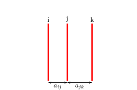
Figure 1: Three parallel plates. Plates $i$ and $k$ are separated by distances $a_{ij}$ and $a_{jk}$ from the center plate $j$.

The three semitransparent plates $i$, $j$, and $k$, of infinite extent and parallel to the $xy$-plane are described by potentials of the form given in Eq. (36). Without loss of generality we assume that $a_{i}<a_{j}<a_{k}$ (see FIG. 1). In the previously introduced notation this implies that $a_{ij}+a_{jk}=a_{ik}$. The vector ${\bf r}(z)$ in Eq. (44) now has three components.

The dimensionally reduced three-body transition matrix is obtained by solving Eq. (29) for $X_{i[jk]}$ using the $X_{ij}$ of Eq. (45). For three semitransparent parallel plates one finds that,

$$X_{i[jk]}X_{jk}=\frac{1}{\Delta_{ijk}},\qquad\Delta_{ijk}=1-\bar{t}_{i}\bar{r}_{ij}\bar{t}_{j}\bar{r}_{ji}-\bar{t}_{j}\bar{r}_{jk}\bar{t}_{k}\bar{r}_{kj}-\bar{t}_{k}\bar{r}_{ki}\bar{t}_{i}\bar{r}_{ik}+2\bar{t}_{i}\bar{r}_{ij}\bar{t}_{j}\bar{r}_{jk}\bar{t}_{k}\bar{r}_{ki}.$$ (50)

Using Eq. (50) in Eq. (28) we obtain

$${\bf t}_{ijk}=\frac{2\kappa}{\Delta_{ijk}}\left[\begin{array}[]{ccc}\bar{t}_{i}\Delta_{jk}&-\bar{t}_{i}\bar{r}_{ij[k]}\bar{t}_{j}&-\bar{t}_{i}\bar{r}_{ik[j]}\bar{t}_{k}\\[5.69054pt] -\bar{t}_{j}\bar{r}_{ji[k]}\bar{t}_{i}&\bar{t}_{j}\Delta_{ki}&-\bar{t}_{j}\bar{r}_{jk[i]}\bar{t}_{k}\\[5.69054pt] -\bar{t}_{k}\bar{r}_{ki[j]}\bar{t}_{i}&-\bar{t}_{k}\bar{r}_{kj[i]}\bar{t}_{j}&\bar{t}_{k}\Delta_{ij}\end{array}\right],$$ (51)

where

$$\bar{r}_{ij[k]}=\bar{r}_{ij}-\bar{r}_{ik}\bar{t}_{k}\bar{r}_{kj}.$$ (52)

It is apparent from the solutions for the $N=2$ and $N=3$ case that terms contributing to the transition matrix in the multiple scattering expansion depend exponentially on the length of the path of propagation. Expanding the inverse determinants $\Delta_{ij}$ and $\Delta_{ijk}$ gives all paths contributing to the scattering operator. This is particularly transparent in our essentially 1-dimensional example.

From Eq. (33) the dimensionally reduced, irreducible, three-body transition matrix is similarly evaluated as,

$$\Delta{\bf t}_{ijk}=2\kappa\left[\begin{array}[]{ccc}\bar{t}_{i}\left\{1-\frac{1}{\Delta_{ij}}-\frac{1}{\Delta_{ik}}+\frac{\Delta_{jk}}{\Delta_{ijk}}\right\}&\bar{t}_{i}\left\{\frac{\bar{r}_{ij}}{\Delta_{ij}}-\frac{\bar{r}_{ij[k]}}{\Delta_{ijk}}\right\}\bar{t}_{j}&\bar{t}_{i}\left\{\frac{\bar{r}_{ik}}{\Delta_{ik}}-\frac{\bar{r}_{ik[j]}}{\Delta_{ijk}}\right\}\bar{t}_{k}\\[8.53581pt] \bar{t}_{j}\left\{\frac{\bar{r}_{ji}}{\Delta_{ji}}-\frac{\bar{r}_{ji[k]}}{\Delta_{ijk}}\right\}\bar{t}_{i}&\bar{t}_{j}\left\{1-\frac{1}{\Delta_{ji}}-\frac{1}{\Delta_{jk}}+\frac{\Delta_{ik}}{\Delta_{ijk}}\right\}&\bar{t}_{j}\left\{\frac{\bar{r}_{jk}}{\Delta_{jk}}-\frac{\bar{r}_{jk[i]}}{\Delta_{ijk}}\right\}\bar{t}_{k}\\[8.53581pt] \bar{t}_{k}\left\{\frac{\bar{r}_{ki}}{\Delta_{ki}}-\frac{\bar{r}_{ki[j]}}{\Delta_{ijk}}\right\}\bar{t}_{i}&\bar{t}_{k}\left\{\frac{\bar{r}_{kj}}{\Delta_{kj}}-\frac{\bar{r}_{kj[i]}}{\Delta_{ijk}}\right\}\bar{t}_{j}&\bar{t}_{k}\left\{1-\frac{1}{\Delta_{ki}}-\frac{1}{\Delta_{kj}}+\frac{\Delta_{ij}}{\Delta_{ijk}}\right\}\end{array}\right].$$ (53)

It is interesting to consider the situation when Dirichlet boundary conditions hold on the $j$-th plate between the other two plates. Taking the limit $\bar{t}_{j}\to\bar{t}_{j}^{D}=1$, the determinant for three parallel plates is found to factorize into a product of two-body determinants,

$$\Delta_{i\infty k}=\Delta_{i\infty}\Delta_{k\infty}=(1-\bar{t}_{i}\,e^{-2\kappa a_{ij}})(1-\bar{t}_{k}\,e^{-2\kappa a_{jk}}),$$ (54)

where replacing the subscript of a plate by $\infty$ denotes Dirichlet boundary conditions on that plate. In this situation, $\bar{r}_{ik[\infty]}=(1-\bar{t}_{j}^{D})\bar{r}_{ik}=0$, $\bar{r}_{i\infty[k]}=e^{\kappa a_{ij}}\Delta_{k\infty}$, $\bar{r}_{k\infty[i]}=e^{\kappa a_{jk}}\Delta_{i\infty}$, and Eq. (51) simplifies to

$${\bf t}_{i\infty k}=2\kappa\left[\begin{array}[]{ccc}\bar{t}_{i}\frac{1}{\Delta_{i\infty}}&-\bar{t}_{i}\frac{\bar{r}_{ij}}{\Delta_{i\infty}}&0\\[5.69054pt] -\frac{\bar{r}_{ji}}{\Delta_{\infty i}}\bar{t}_{i}&\frac{1}{\Delta_{i\infty}}+\frac{1}{\Delta_{k\infty}}-1&-\frac{\bar{r}_{jk}}{\Delta_{k\infty}}\bar{t}_{k}\\[5.69054pt] 0&-\bar{t}_{k}\frac{\bar{r}_{kj}}{\Delta_{k\infty}}&\bar{t}_{k}\frac{1}{\Delta_{k\infty}}\end{array}\right].$$ (55)

This leads to the observation that

$${\bf t}_{i\infty k}={\bf t}_{i\infty}+{\bf t}_{k\infty}-{\bf t}_{j}^{D}={\bf t}_{i}+{\bf t}_{j}^{D}+{\bf t}_{k}+\Delta{\bf t}_{i\infty}+\Delta{\bf t}_{k\infty}.$$ (56)

Comparing Eq. (56) with the decomposition of the three-body transition matrix into irreducible one–and two-body parts in Eq. (31) this implies

$$\Delta{\bf t}_{i\infty k}+\Delta{\bf t}_{ik}=0,$$ (57)

which confirms the notion that modes in the two half-spaces on either side of a Dirichlet plate are independent and that correlations between them must vanish. The irreducible three-body correlations in this limit therefore must cancel irreducible two-body correlations between objects on opposite sides of the plate. Taking the Dirichlet limit on the central plate in Eq. (53) this is verified explicitly,

$$\Delta{\bf t}_{i\infty k}=2\kappa\left[\begin{array}[]{ccc}\bar{t}_{i}\left\{1-\frac{1}{\Delta_{ik}}\right\}&0&\bar{t}_{i}\frac{\bar{r}_{ik}}{\Delta_{ik}}\bar{t}_{k}\\[8.53581pt] 0&0&0\\[8.53581pt] \bar{t}_{k}\frac{\bar{r}_{ki}}{\Delta_{ki}}\bar{t}_{i}&0&\bar{t}_{k}\left\{1-\frac{1}{\Delta_{ki}}\right\}\end{array}\right]=-\Delta{\bf t}_{ik},$$ (58)

where we have used Eq. (48).

Let us finally consider the case when Dirichlet boundary conditions are imposed on all three plates. The three-body determinant again factorizes, $\Delta_{ijk}^{D}=\Delta_{ij}^{D}\Delta_{jk}^{D}=(1-e^{-2\kappa a_{ij}})(1-e^{-2\kappa a_{jk}})$, and

$${\bf t}_{ijk}^{D}=2\kappa\left[\begin{array}[]{ccc}\dfrac{e^{\kappa a_{ij}}}{2\sinh\kappa a_{ij}}&-\dfrac{1}{2\sinh\kappa a_{ij}}&0\\[8.53581pt] -\dfrac{1}{2\sinh\kappa a_{ij}}&\dfrac{e^{\kappa a_{ij}}}{2\sinh\kappa a_{ij}}+\dfrac{e^{\kappa a_{jk}}}{2\sinh\kappa a_{jk}}-1&-\dfrac{1}{2\sinh\kappa a_{jk}}\\[8.53581pt] 0&-\dfrac{1}{2\sinh\kappa a_{jk}}&\dfrac{e^{\kappa a_{jk}}}{2\sinh\kappa a_{jk}}\end{array}\right]={\bf t}_{i}^{D}+{\bf t}_{j}^{D}+{\bf t}_{k}^{D}+\Delta{\bf t}_{ij}^{D}+\Delta{\bf t}_{jk}^{D},$$ (59)

in the limit of three Dirichlet plates. This implies $\Delta{\bf t}_{ijk}^{D}+\Delta{\bf t}_{ik}^{D}=0$, and is explicitly verified by Eq. (53) or Eq. (58),

$$\Delta{\bf t}_{ijk}^{D}=-\frac{\kappa}{\sinh\kappa a_{ik}}\left[\begin{array}[]{ccc}e^{-\kappa a_{ik}}&0&-1\\ 0&0&0\\ -1&0&e^{-\kappa a_{ik}}\end{array}\right]=-\Delta{\bf t}_{ik}^{D},$$ (60)

using Eq. (49).

IV Many-body Casimir energies

Casimir energies are finite parts of the vacuum energy that describe its dependence on configurations of macroscopic objects. The interaction of classical objects with quantized fields at low energies can be described by background potentials. It is known Deutsch:1978sc ; kirsten2002spectral ; Fulling:1989nb ; Bordag:PRD70.045003 ; Schaden:2010wv that such a semiclassical description for the interaction with a quantized field suffers of (local) ultraviolet divergences. A proper treatment of the interaction at high energies requires modeling of the quantum fluctuations associated with the objects. One fortunately sometimes is able to isolate parts of the vacuum energy that depend only on global changes of the system and can be reliably computed in semiclassical approximation. In the following we systematically determine irreducible parts of the vacuum energy for a given number of classical objects. These irreducible $N$-body Casimir energies diverge only if all $N$ potentials describing the classical objects have a region of common support Schaden:2010wv .

Let $E_{0}$ be the (infinite) vacuum energy associated with zero-point fluctuations of a massless scalar field in the absence of all background potentials, $V_{i}({\bf x})$. The change in vacuum energy in the presence of $N$ objects associated with the background potential, $V=\sum_{i}V_{i}$, can be derived using field theory techniques, for example in Bordag:1992cm ; CaveroPelaez:2008tj , to be

$$E_{1\ldots N}-E_{0}=-\frac{1}{2}\int_{-\infty}^{\infty}\frac{d\zeta}{2\pi}\,2\zeta^{2}\,\text{Tr}\,(G_{1\ldots N}-G_{0})=-\frac{1}{2}\int_{-\infty}^{\infty}\frac{d\zeta}{2\pi}\,\text{Tr}\ln\tilde{G}_{1\ldots N}=-\frac{1}{2}\int_{-\infty}^{\infty}\frac{d\zeta}{2\pi}\,\text{Tr}\ln(1-\tilde{T}_{1\ldots N}).$$ (61)

These expressions have recently been dubbed the Trace-G-formula and Trace-Log-G-formula respectively. For frequency independent potentials, the relation between them is established by differentiating Eq. (7),

$$-\frac{d}{d\zeta^{2}}\,G=GG,$$ (62)

and ignoring a boundary term.

To proceed further we generalize Eqs. (26) and (34) and decompose a Green’s function involving $N$ potentials into irreducible $N$-body parts,

$$G_{1\ldots N}=G_{0}+\sum_{i}\Delta G_{i}+\sum_{i<j}\Delta G_{ij}+\dots.$$ (63)

Using Eq. (62), the irreducible one–two–and three-body parts of the Green’s functions can be written in the form ($i\neq j\neq k$)

$$\Delta G_{i} = G_{i}-G_{0}=-\frac{d}{d\zeta^{2}}\,\ln\frac{G_{i}}{G_{0}},$$ (64a)

$$\Delta G_{ij} = G_{ij}-\Delta G_{i}-\Delta G_{j}=-\frac{d}{d\zeta^{2}}\,\ln\frac{G_{ij}G_{0}}{G_{i}G_{j}},$$ (64b)

$$\Delta G_{ijk} = G_{ijk}-\Delta G_{ij}-\Delta G_{jk}-\Delta G_{ki}-\Delta G_{i}-\Delta G_{j}-\Delta G_{k}=-\frac{d}{d\zeta^{2}}\,\ln\frac{G_{ijk}G_{i}G_{j}G_{k}}{G_{ij}G_{jk}G_{ki}G_{0}},$$ (64c)

which is a (cascading) recursive definition that can be extended to higher $N$.

Eqs. (61) and (63) imply a corresponding decomposition of the vacuum energy into irreducible $N$-body contributions,

$$E_{1\ldots N}=E_{0}+\sum_{i}\Delta E_{i}+\sum_{i<j}\Delta E_{ij}+\dots,$$ (65)

where

$$\Delta E_{1\ldots N}=-\frac{1}{2}\int_{-\infty}^{\infty}\frac{d\zeta}{2\pi}\,2\zeta^{2}\,\text{Tr}\,\Delta G_{1\ldots N}.$$ (66)

As shown in Schaden:2010wv , and as will be explicitly verified in examples below, the irreducible $N$-body contribution to the vacuum energy diverges only if all $N$ potentials have a common support. One-body vacuum energies thus are generically divergent, whereas two-body Casimir energies diverge only if the two bodies intersect (and thus could be viewed as one). More interestingly though, three-body Casimir energies diverge only when all three objects have a common intersection–the three bodies need not be mutually disjoint and could, for instance, be arranged to form a triangle.

Eq. (13) relates the irreducible $N$-body contribution of the Green’s functions to the irreducible $N$-body transition matrix,

$$\text{Tr}\,\Delta G_{1\ldots N}=-\text{Tr}\,\Delta T_{1\ldots N}G_{0}G_{0}=\text{Tr}\,\Delta T_{1\ldots N}\frac{d}{d\zeta^{2}}G_{0}.$$ (67)

The support of delta-function potentials $V_{i}$ is restricted to the surface $S_{i}$ of the $i$-th object and components of the transition-matrix at most have support on the union of two such surfaces. It is therefore convenient to formally define a vector ${\bf R}({\bf x})$, and a matrix ${\bf R}$, with components

$${\bf R}_{i}({\bf x}):=G_{0}({\bf x}-{\bf y})\big{|}_{{\bf y}\in S_{i}},\qquad{\bf R}_{ij}:=G_{0}({\bf x}-{\bf y})\big{|}_{\genfrac{}{}{0.0pt}{}{{\bf x}\in S_{i}}{{\bf y}\in S_{j}}}.$$ (68)

Using these definitions in Eq. (62) we have

$$-\frac{d}{d\zeta^{2}}{\bf R}=\int d^{3}x\,{\bf R}({\bf x})\cdot{\bf R}({\bf x})^{T}.$$ (69)

Writing the irreducible $N$-body transition operator in Eq. (67) in matrix notation and using Eq. (69), we express the irreducible $N$-body contribution to the vacuum energy of Eq. (66) in the form

$$\Delta E_{1\ldots N}=-\frac{1}{2}\int_{-\infty}^{\infty}\frac{d\zeta}{2\pi}\,2\zeta^{2}\,\text{Tr}\left[\Delta{\bf T}_{1\ldots N}\cdot\frac{d}{d\zeta^{2}}{\bf R}\right].$$ (70)

The trace in the last expression is over matrix indices and includes integrals over the lower dimensional surfaces of the associated objects. Note also that Eq. (70) involves the irreducible $N$-body transition matrix, ${\bf T}_{1\ldots N}$, not its partly amputated cousin $\tilde{\bf T}_{1\ldots N}$.

V Casimir energies for parallel semitransparent $\delta$-plates

We illustrate this formalism by evaluating the irreducible (scalar) Casimir energy for semitransparent parallel plates described by potentials of the form given in Eq. (36). Exploiting translational invariance parallel to the plates in Eq. (70), the irreducible $N$-body Casimir energy per unit area is described by dimensionally reduced quantities

$$\frac{\Delta E_{1\ldots N}}{L_{x}L_{y}}=-\frac{1}{6\pi^{2}}\int_{0}^{\infty}\kappa^{4}d\kappa\,\text{Tr}\left[\Delta{\bf t}_{1\ldots N}\cdot\frac{d}{d\zeta^{2}}{\bf r}\right],$$ (71)

where $L_{x}$ and $L_{y}$ are the (infinite) lengths of the plates in $x$ and $y$ direction, respectively. The integrals on $\zeta$, $k_{x}$, and $k_{y}$, are performed using polar varibales, which effectively amounts to replacing $\zeta^{2}\to 2\kappa^{2}/3$, where $\kappa$ was defined after Eq. (37). The dimensionally reduced transition matrices, $\Delta{\bf t}_{1\ldots N}$, for $N=2$ and $N=3$ are, respectively, given by Eqs. (48) and (53). The derivative of the dimensionally reduced free Green’s function in this case is the matrix

$$-\frac{d}{d\zeta^{2}}{\bf r}=\int_{-\infty}^{\infty}dz\,{\bf r}(z)\cdot{\bf r}(z)^{T}=\frac{2}{(2\kappa)^{3}}\left[\begin{array}[]{cccc}1&(1+\kappa a_{12})\,e^{-\kappa a_{12}}&\cdots&(1+\kappa a_{1N})\,e^{-\kappa a_{1N}}\\[2.84526pt] (1+\kappa a_{21})\,e^{-\kappa a_{21}}&1&\cdots&(1+\kappa a_{2N})\,e^{-\kappa a_{2N}}\\[2.84526pt] \vdots&\vdots&\ddots&\vdots\\[2.84526pt] (1+\kappa a_{N1})\,e^{-\kappa a_{N1}}&(1+\kappa a_{N2})\,e^{-\kappa a_{N2}}&\cdots&1\end{array}\right],$$ (72)

where $a_{ij}$ is the distance between the $i$-th and $j$-th parallel plate defined previously.

V.1 $N=1,2$: Irreducible one–and two-body Casimir energy for semitransparent plates

The irreducible one-body vacuum energy per unit area associated with the $i$-th plate diverges. Eq. (71) gives it as the integral

$$\frac{\Delta E_{i}}{L_{x}L_{y}}=\frac{1}{12\pi^{2}}\int_{0}^{\infty}\kappa^{2}d\kappa\,\bar{t}_{i},$$ (73)

with $\bar{t}_{i}$ defined in Eq. (42). The one-body vacuum energies are ultra-violet divergent at any non-vanishing coupling, but do not depend on the relative position of the plates and therefore do not contribute to forces between them.

The irreducible two-body Casimir energy per unit area associated with plates $i$ and $j$ is obtained by inserting Eqs. (48) and (72) (for $N=2$) in Eq. (71),

$$\frac{\Delta E_{ij}}{L_{x}L_{y}}=-\frac{1}{12\pi^{2}}\int_{0}^{\infty}\kappa^{2}d\kappa\left[\frac{1}{\Delta_{ij}}-1\right]\big{[}2\kappa a_{ij}+(1-\bar{t}_{i})+(1-\bar{t}_{j})\big{]},$$ (74)

where the two-body determinant is given by Eq. (45). Eq. (74) for the Casimir interaction energy of two semitransparent plates was obtained previously in Bordag:1992cm . In the Dirichlet limit, $\bar{t}_{i}\to 1$, Eq. (74) simplifies to the well known Casimir energy for a massless scalar field satisfying Dirichlet boundary conditions on a pair of parallel plates,

$$\frac{\Delta E_{ij}^{D}}{L_{x}L_{y}}=-\frac{1}{12\pi^{2}}\int_{0}^{\infty}\kappa^{2}d\kappa\frac{2\kappa a_{ij}}{e^{2\kappa a_{ij}}-1}=-\frac{\pi^{2}}{1440}\frac{1}{a_{ij}^{3}}.$$ (75)

Eqs. (74) and (75) are finite and negative for two disjoint plates.

V.2 $N=3$: Three-body Casimir energy for three parallel plates

The irreducible three-body Casimir energy of three plates is similarly obtained by inserting Eqs. (53) and (72) (for $N=3$) in Eq. (71),

$$\frac{\Delta E_{ijk}}{L_{x}L_{y}} = \frac{1}{12\pi^{2}}\int_{0}^{\infty}\kappa^{2}d\kappa\bigg{[}\bar{t}_{i}\left\{1-\frac{1}{\Delta_{ij}}-\frac{1}{\Delta_{ik}}+\frac{\Delta_{jk}}{\Delta_{ijk}}\right\}+2(1+\kappa a_{jk})\left\{\frac{1}{\Delta_{jk}}-1\right\}\left\{1-\bar{r}_{jk[i]}e^{\kappa a_{jk}}\frac{\Delta_{jk}}{\Delta_{ijk}}\right\}$$ (76)

$$\hskip 71.13188pt+\bar{t}_{j}\left\{1-\frac{1}{\Delta_{ji}}-\frac{1}{\Delta_{jk}}+\frac{\Delta_{ik}}{\Delta_{ijk}}\right\}+2(1+\kappa a_{ik})\left\{\frac{1}{\Delta_{ik}}-1\right\}\left\{1-\bar{r}_{ik[j]}e^{\kappa a_{ik}}\frac{\Delta_{ik}}{\Delta_{ijk}}\right\}$$

$$\hskip 71.13188pt+\bar{t}_{k}\left\{1-\frac{1}{\Delta_{ki}}-\frac{1}{\Delta_{kj}}+\frac{\Delta_{ij}}{\Delta_{ijk}}\right\}+2(1+\kappa a_{ij})\left\{\frac{1}{\Delta_{ij}}-1\right\}\left\{1-\bar{r}_{ij[k]}e^{\kappa a_{ij}}\frac{\Delta_{ij}}{\Delta_{ijk}}\right\}\bigg{]}.$$

When Dirichlet boundary conditions are imposed on the central $j$-th plate, the relation between irreducible two–and three-body transition matrices noted in Eq. (57) implies a corresponding relation between two–and three-body Casimir energies,

$$\Delta E_{i\infty k}+\Delta E_{ik}=0.$$ (77)

This is explicitly verified by using the factorization of the three-body determinant in Eq. (54) and the Dirichlet limits for $\bar{r}_{ij[k]}$ given after Eq. (54) in Eq. (76), and identifying the irreducible two-body energy of Eq. (74) in the result.

In the Dirichlet limit for all three plates the irreducible three-body Casimir energy cancels the well-known two-body interaction between the outer Dirichlet plates,

$$\frac{\Delta E_{ijk}^{D}}{L_{x}L_{y}}=\frac{\pi^{2}}{1440}\frac{1}{a_{ik}^{3}}=-\frac{\Delta E_{ik}^{D}}{L_{x}L_{y}},$$ (78)

where $a_{ik}$ is the distance between the outer plates.

This cancellation is to be expected on physical grounds and serves to check the calculation. For semitransparent plates the cancellation is not complete and the irreducible three-body contribution to the total Casimir energy can be significant for parallel plates. Note that the sign of the irreducible $N$-body contribution to the scalar Casimir energy alternates. Although not apparent from the expression of Eq. (76), this irreducible three-body contribution to the Casimir energy is positive for any positive couplings $\lambda_{1},\lambda_{2},\lambda_{3}$ and any relative position of the three plates. For parallel semitransparent plates we thus verify the more general result obtained in Schaden:2010wv . Also, as discussed in Schaden:2010wv and noted previously, the three-plate Casimir energy diverges only if all three plates coincide.

In the following we will see that these generic results for the sign and analyticity of the three-body scalar Casimir energy hold in the limit where two of the three potentials are weak and need only be accounted for to leading order.

VI Three-body Scalar Casimir interaction for semiweak coupling

We now consider irreducible vacuum energies for three bodies when two of the three potentials, $V_{1}$ and $V_{2}$, are weak and need only be taken to leading order. No restriction is imposed on the potential $V_{3}$ describing the third body. To the leading order we thus approximate $T_{1}\sim V_{1}$ and $T_{2}\sim V_{2}$ in Eq. (9). The three-body transition matrix of Eq. (28) in this semiweak approximation simplifies to

$$\tilde{\bf T}_{123}^{W}=\left[\begin{array}[]{ccc}1&0&0\\ 0&1&0\\ 0&0&X_{3[12]}^{W}\end{array}\right]\left[\begin{array}[]{ccc}\tilde{V}_{1}&-\tilde{V}_{1}(1-\tilde{T}_{3})\tilde{V}_{2}&-\tilde{V}_{1}(1-\tilde{V}_{2}+\tilde{T}_{3}\tilde{V}_{2})\tilde{T}_{3}\\ -\tilde{V}_{2}(1-\tilde{T}_{3})\tilde{V}_{1}&\tilde{V}_{2}&-\tilde{V}_{2}(1-\tilde{V}_{1}+\tilde{T}_{3}\tilde{V}_{1})\tilde{T}_{3}\\ -\tilde{T}_{3}(1-\tilde{V}_{2})\tilde{V}_{1}&-\tilde{T}_{3}(1-\tilde{V}_{1})\tilde{V}_{2}&\tilde{T}_{3}\end{array}\right].$$ (79)

Here $X_{3[12]}^{W}$ satisfies Eq. (29), which to leading semiweak approximation is solved by

$$X_{3[12]}^{W}=1+\tilde{T}_{3}(1-\tilde{V}_{1})\tilde{V}_{2}+\tilde{T}_{3}(1-\tilde{V}_{2})\tilde{V}_{1}+\tilde{T}_{3}\tilde{V}_{1}\tilde{T}_{3}\tilde{V}_{2}+\tilde{T}_{3}\tilde{V}_{2}\tilde{T}_{3}\tilde{V}_{1}.$$ (80)

The transition matrix in semiweak approximation of Eq. (79) may again be decomposed into its irreducible one–two–and three-body parts, leading to the semiweak version of Eq. (31). From Eq. (25) the irreducible two-body transition matrices in semiweak approximation are,

$$\Delta\tilde{\bf T}_{12}^{W}=\left[\begin{array}[]{cc}0&-\tilde{V}_{1}\tilde{V}_{2}\\ -\tilde{V}_{2}\tilde{V}_{1}&0\end{array}\right],\qquad\Delta\tilde{\bf T}_{i3}^{W}=\left[\begin{array}[]{cc}0&-\tilde{V}_{i}\tilde{T}_{3}\\ -\tilde{T}_{3}\tilde{V}_{i}&\tilde{T}_{3}\tilde{V}_{i}\tilde{T}_{3}\end{array}\right],$$ (81)

with $i=1,2$. Similarly approximating Eq. (33), the three-body transition matrix in semiweak approximation becomes,

$$\Delta\tilde{\bf T}_{123}^{W}=\left[\begin{array}[]{ccc}0&\tilde{V}_{1}\tilde{T}_{3}\tilde{V}_{2}&\tilde{V}_{1}\tilde{G}_{3}\tilde{V}_{2}\tilde{T}_{3}\\ \tilde{V}_{2}\tilde{T}_{3}\tilde{V}_{1}&0&\tilde{V}_{2}\tilde{G}_{3}\tilde{V}_{1}\tilde{T}_{3}\\ \tilde{T}_{3}\tilde{V}_{2}\tilde{G}_{3}\tilde{V}_{1}&\tilde{T}_{3}\tilde{V}_{1}\tilde{G}_{3}\tilde{V}_{2}&-\tilde{T}_{3}\tilde{V}_{1}\tilde{G}_{3}\tilde{V}_{2}\tilde{T}_{3}-\tilde{T}_{3}\tilde{V}_{2}\tilde{G}_{3}\tilde{V}_{1}\tilde{T}_{3}\end{array}\right],$$ (82)

where $\tilde{G}_{3}=1-\tilde{T}_{3}$.

Casimir energies in the semiweak approximation are obtained using Eqs. (66) and (67). Inserting Eq. (81) in Eq. (67) we have to this approximation,

$$-\text{Tr}\,\Delta G_{12}^{W}=\text{Tr}\left[\Delta{\bf T}_{12}^{W}\cdot\frac{d}{d\zeta^{2}}{\bf R}\right] = \frac{d}{d\zeta^{2}}\text{Tr}\Big{[}G_{0}V_{1}G_{0}V_{2}\Big{]},$$ (83a)

$$-\text{Tr}\,\Delta G_{i3}^{W}=\text{Tr}\left[\Delta{\bf T}_{i3}^{W}\cdot\frac{d}{d\zeta^{2}}{\bf R}\right] = \frac{d}{d\zeta^{2}}\text{Tr}\Big{[}G_{0}V_{i}G_{0}T_{3}\Big{]},\qquad(i=1,2).$$ (83b)

The corresponding irreducible three-body contribution using Eq. (82) in Eq. (67) is

$$-\text{Tr}\,\Delta G_{123}^{W}=\text{Tr}\left[\Delta{\bf T}_{123}^{W}\cdot\frac{d}{d\zeta^{2}}{\bf R}\right]=-\frac{d}{d\zeta^{2}}\text{Tr}\Big{[}G_{0}V_{1}G_{0}T_{3}G_{0}V_{2}+G_{0}V_{2}G_{0}T_{3}G_{0}V_{1}-G_{0}T_{3}G_{0}V_{1}G_{0}T_{3}G_{0}V_{2}\Big{]}.$$ (84)

Inserting Eq. (83) in Eq. (66), and integrating by parts, the irreducible two-body Casimir energies in semiweak approximation are

$$\Delta E_{12}^{W} = -\frac{1}{2}\int_{-\infty}^{\infty}\frac{d\zeta}{2\pi}\,\text{Tr}\big{[}G_{0}V_{1}G_{0}V_{2}\big{]},$$ (85a)

$$\Delta E_{i3}^{W} = -\frac{1}{2}\int_{-\infty}^{\infty}\frac{d\zeta}{2\pi}\,\text{Tr}\big{[}G_{0}V_{i}G_{0}T_{3}\big{]},\qquad(i=1,2),$$ (85b)

verifying results reported in Milton:2007wz . The corresponding irreducible three-body contribution to the Casimir energy in semiweak approximation using Eq. (84) in Eq. (66) is

$$\Delta E_{123}^{W}=\frac{1}{2}\int_{-\infty}^{\infty}\frac{d\zeta}{2\pi}\,\text{Tr}\big{[}G_{0}V_{1}G_{0}T_{3}G_{0}V_{2}+G_{0}V_{2}G_{0}T_{3}G_{0}V_{1}-G_{0}T_{3}G_{0}V_{1}G_{0}T_{3}G_{0}V_{2}\big{]}.$$ (86)

In the following we evaluate Eqs. (85) and (86) for some special cases.

VI.1 Weak point potentials

Weak point potentials of the form,

$$V_{i}({\bf x})=\lambda_{i}\delta({\bf x}-{\bf x}_{i}),$$ (87)

for $i=1,2$, allow one to explicitly perform the integrals in Eqs. (85) and (86). In this case we have

$$\Delta E_{12}^{W}=-\frac{\lambda_{1}\lambda_{2}}{2}\int_{-\infty}^{\infty}\frac{d\zeta}{2\pi}\,\big{[}G_{0}({\bf x}_{1}-{\bf x}_{2})\big{]}^{2}<0,$$ (88)

and, using Eq. (8) in Eq. (85b),

$$\Delta E_{i3}^{W}=-\frac{\lambda_{i}}{2}\int_{-\infty}^{\infty}\frac{d\zeta}{2\pi}\,\Big{\{}G_{0}(0)-G_{3}({\bf x}_{i},{\bf x}_{i})\Big{\}}<0,\qquad(i=1,2),$$ (89)

because the integrand in braces is positive for positive $V_{3}$. The irreducible two-body contributions to the vacuum energy thus are negative for weak point potentials. We similarly obtain that the irreducible three-body correction to the vacuum energy,

$$\Delta E_{123}^{W}=\frac{\lambda_{1}\lambda_{2}}{2}\int_{-\infty}^{\infty}\frac{d\zeta}{2\pi}\,\Big{\{}\big{[}G_{0}({\bf x}_{1}-{\bf x}_{2})\big{]}^{2}-\big{[}G_{3}({\bf x}_{1},{\bf x}_{2})\big{]}^{2}\Big{\}}>0,$$ (90)

in this case is positive for any (positive) potential $V_{3}$. Note that the irreducible three-body Casimir energy in semiweak approximation diverges only if ${\bf x}_{1}={\bf x}_{2}$ is in the support of $V_{3}$.

The pattern in the sign of the irreducible $N$-body contribution is consistent with the findings of Schaden:2010wv . Furthermore, since any positive potential is a (positive) superposition of point potentials, this pattern of the signs of irreducible $N$-body contributions extend to any shape of the objects in semiweak approximation. This is explicitly verified by the following examples.

VI.2 Weak potentials with translational symmetry parallel to a Dirichlet plate

We consider a Dirichlet plate and weak potentials that do not depend on the Cartesian coordinate $x$,

$$V_{i}=V_{i}(y,z),\quad\text{for}\quad i=1,2;\quad\text{and}\quad V_{3}=\lambda_{3}\,\delta(z-a_{3}),\quad\text{with}\quad\lambda_{3}\to\infty.$$ (91)

To evaluate Eqs. (85) and (86) for such potentials we require the operator $G_{0}T_{3}^{D}G_{0}$ for a Dirichlet plate. In order to exploit the translational symmetry in $x$-direction we write the solution to Eq. (6) for the free Green’s function in the form

$$G_{0}(|{\bf x}_{1}-{\bf x}_{2}|;\zeta)=\int\frac{d^{2}k}{(2\pi)^{2}}\,e^{i{\bf k}\cdot({\bf x}_{1}-{\bf x}_{2})_{\perp}}\frac{e^{-\kappa|z_{1}-z_{2}|}}{2\kappa}=\int_{-\infty}^{\infty}\frac{dk_{x}}{2\pi}\,e^{ik_{x}(x_{1}-x_{2})}\frac{K_{0}(\bar{\kappa}\,d_{12})}{2\pi}=\frac{e^{-|\zeta||{\bf x}_{1}-{\bf x}_{2}|}}{4\pi|{\bf x}_{1}-{\bf x}_{2}|},$$ (92)

where $d_{12}=\sqrt{(y_{1}-y_{2})^{2}+(z_{1}-z_{2})^{2}}$ is the projected distance in the $x_{1}=x_{2}$ plane, and $\bar{\kappa}^{2}=k_{x}^{2}+\zeta^{2}$. $K_{0}(x)$ is the modified Bessel function of zero order. Note that $\kappa$ defined after Eq. (37) satisfies $\kappa^{2}=\bar{\kappa}^{2}+k_{y}^{2}$. Using the first equality of Eq. (92) and the dimensionally reduced transition matrix of a Dirichlet plate given in Eq. (42) one can show that

$$-\Delta G_{3}^{D}({\bf x}_{1},{\bf x}_{2};\zeta)=[G_{0}T_{3}^{D}G_{0}]({\bf x}_{1},{\bf x}_{2};\zeta)=G_{0}(|{\bf x}_{1}-\bar{\bf x}_{2}|;\zeta)=\int_{-\infty}^{\infty}\frac{dk_{x}}{2\pi}\,e^{ik_{x}(x_{1}-x_{2})}\frac{K_{0}(\bar{\kappa}\,\bar{d}_{12})}{2\pi},$$ (93)

where $\bar{\bf x}_{2}=(x_{2},y_{2},-z_{2}+2a_{3})$, and $\bar{d}_{12}$ is the length of the shortest path between ${\bf x}_{1}$ and ${\bf x}_{2}$ in the $(x_{1}=x_{2})$-plane that reflects off the Dirichlet plate. For a Dirichlet plate at $z=a_{3}$, this distance is given by $\bar{d}^{2}_{12}=(y_{1}-y_{2})^{2}+(|z_{1}-a_{3}|+|z_{2}-a_{3}|)^{2}$. A geometrical interpretation of $d_{12}$ and $\bar{d}_{12}$ is shown in FIG. 2. Substituting Eq. (93) in Eq. (8) leads to

$$G_{3}^{D}({\bf x}_{1},{\bf x}_{2};\zeta)=G_{0}(|{\bf x}_{1}-{\bf x}_{2}|;\zeta)-G_{0}(|{\bf x}_{1}-\bar{\bf x}_{2}|;\zeta),$$ (94)

which is anti-symmetric under reflection about the Dirichlet plate. Note that if ${\bf x}_{1}$ and ${\bf x}_{2}$ are on opposite sides of the plate, $\bar{d}_{12}=d_{12}$, and $G_{3}^{D}$ vanishes.

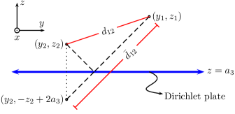
Figure 2: The distances $d_{12}$ and $\bar{d}_{12}$. The effective distance $\bar{d}_{12}$ is the shortest distance between the two points for a path that reflects off the Dirichlet plate at $z=a_{3}$. It also is the shortest distance between $(y_{1},z_{1})$ and a mirror image of the point $(y_{2},z_{2})$ with respect to the $z=a_{3}$ line.

Substituting Eq. (92) for the free Green’s functions, and Eq. (93) for the irreducible Green’s function of a Dirichlet plate in Eqs. (85) and using the identity

$$\int_{0}^{\infty}\bar{\kappa}\,d\bar{\kappa}\,K_{0}(\bar{\kappa}x)=\frac{1}{x^{2}},$$ (95)

the irreducible two-body Casimir energies per unit length in semiweak approximation for potentials with translational symmetry are

$$\frac{\Delta E_{12}^{W}}{L_{x}} = -\frac{1}{32\pi^{3}}\int d^{2}r_{1}\int d^{2}r_{2}\frac{V_{1}({\bf r}_{1})V_{2}({\bf r}_{2})}{d_{12}^{2}},$$ (96a)

$$\frac{\Delta E_{i3}^{W}}{L_{x}} = -\frac{1}{32\pi^{2}}\int d^{2}r\frac{V_{i}({\bf r})}{|z|^{2}},\qquad(i=1,2).$$ (96b)

The Casimir energy in Eq. (96a) for two weakly interacting objects with translational symmetry was previously obtained in Wagner:2008qq . The Casimir energy for a Dirichlet plate weakly interacting with an object possessing translational symmetry was obtained in Milton:2007wz , but was given as a series involving modified Bessel functions. The expression in Milton:2007wz generally is much harder to evaluate than Eq. (96b). The simplification in Eq. (96b) was achieved by using the effective Green’s function for a Dirichlet plate in Eq. (93). For many potentials, the evaluation of the Casimir energy by Eq. (96b) is immediate. We can for example calculate the two-body Casimir energy for a cylinder of radius $a$, described by the weak potential $V_{\text{cyl}}=\lambda\,\delta(r-a)$, interacting with a Dirichlet plate positioned at $z=R>a$. From Eq. (96b) one readily finds,

$$\frac{\Delta E_{\text{Cyl-DP}}^{W}}{L_{x}}=-\frac{1}{32\pi^{2}}\int_{0}^{\infty}rdr\int_{0}^{2\pi}d\theta\frac{\lambda\delta(r-a)}{|r\sin\theta-R|^{2}}=-\frac{\lambda a}{16\pi}\frac{1}{R^{2}}\left[1-\frac{a^{2}}{R^{2}}\right]^{-\frac{3}{2}},$$ (97)

which reproduces the expression in Milton:2007wz . A similarly simplified evaluation is expected for an arbitrary surface with translational symmetry weakly interacting with a Dirichlet plate parallel to the symmetry axis.

The irreducible three-body Casimir energies for translationally invariant weak potentials and a Dirichlet plate can be similarly evaluated using Eq. (86). The first two terms in Eq. (86) involve the product of the free Green’s function, $G_{0}$, with the irreducible Green’s function for a Dirichlet plate given in Eq. (93). The last term requires the product of two irreducible one-body Green’s functions. A useful identity for the product of two modified Bessel functions of zeroth order is

$$\int_{0}^{\infty}\bar{\kappa}\,d\bar{\kappa}\,K_{0}(\bar{\kappa}x)K_{0}(\bar{\kappa}y)=\frac{1}{x^{2}-y^{2}}\ln\left(\frac{x}{y}\right)\xrightarrow{x\to y}\frac{1}{2x^{2}}.$$ (98)

Inserting Eqs. (92) and (93) in Eq. (86) to write the Green’s functions in terms of modified Bessel functions, and then using Eq. (98), we obtain

$$\frac{\Delta E_{123}^{W}}{L_{x}}=\frac{1}{32\pi^{3}}\int d^{2}r_{1}\int d^{2}r_{2}\frac{V_{1}({\bf r}_{1})V_{2}({\bf r}_{2})}{\bar{d}_{12}^{2}}\;Q\left(\frac{d_{12}^{2}}{\bar{d}_{12}^{2}}\right),$$ (99)

where the distances $d_{12}$ and $\bar{d}_{12}$ were introduced earlier and are shown in FIG. 2. The function

$$Q(x)=-\frac{2\ln x}{1-x}-1$$ (100)

is bounded by $1\leq Q(x)\leq 1-2\ln x$ in the relevant domain $0<x=\frac{d_{12}^{2}}{\bar{d}_{12}^{2}}<1$. This implies that the three-body Casimir energy of Eq. (99) is always positive and bounded by

$$\frac{1}{32\pi^{3}}\int d^{2}r_{1}\int d^{2}r_{2}\frac{V_{1}({\bf r}_{1})V_{2}({\bf r}_{2})}{\bar{d}_{12}^{2}}\leq\frac{\Delta E_{123}^{W}}{L_{x}}\leq\frac{1}{32\pi^{3}}\int d^{2}r_{1}\int d^{2}r_{2}\frac{V_{1}({\bf r}_{1})V_{2}({\bf r}_{2})}{\bar{d}_{12}^{2}}\left[1-2\ln\left(\frac{d^{2}_{12}}{\bar{d}^{2}_{12}}\right)\right].$$ (101)

$\bar{d}_{12}$ is the distance between a point on the first object and another point on the reflected image of the second object (see FIG. 2). It vanishes only at points where the two weak objects and the Dirichlet plate are concurrent. The irreducible three-body Casimir energy in the semiweak approximation of Eq. (99) thus is finite if the three objects have no point in common. This contribution in particular does not diverge as the objects approach the plate or each other, corroborating the findings in Schaden:2010wv . Note that the lower bound in Eq. (101) is the two-body Casimir energy between weak potentials of Eq. (96a), but with the reflected object ($d_{12}\to\bar{d}_{12}$) and of opposite sign. The irreducible three-body Casimir energy approaches the lower bound for $\frac{d_{12}^{2}}{\bar{d}_{12}^{2}}\sim 1$ and thus partially cancels the irreducible two-body energy if one or both objects approach the Dirichlet plate. In fact, if the two weakly interacting objects are entirely on opposite sides of the Dirichlet plate, the lower bound is achieved because $\bar{d}_{12}=d_{12}$ and the three-body Casimir energy cancels the two-body interaction energy between them precisely.

The following examples demonstrate the finiteness, sign, and analyticity, of three-body contributions to Casimir energies for cases in which irreducible one–and two-body contributions to the vacuum energy diverge.

VII Triangular-wedge on a Dirichlet plate

We first consider a triangular-wedge with two sides described by weak potentials atop a Dirichlet plate at $z=0$, forming a waveguide of triangular cross-section:

$$V_{1}(y,z) = \lambda_{1}\delta(-z+m_{\alpha}(y-a))\,\theta_{1},\quad\text{with}\quad\theta_{1}\equiv\theta(y-\text{min}[0,a])\,\theta(\text{max}[0,a]-y),$$ (102a)

$$V_{2}(y,z) = \lambda_{2}\delta(-z+m_{\beta}(y-b))\,\theta_{2},\quad\text{with}\quad\theta_{2}\equiv\theta(y-\text{min}[0,b])\,\theta(\text{max}[0,b]-y),$$ (102b)

$$V_{3}(z) = \lambda_{3}\delta(z),\quad\text{with}\quad\lambda_{3}\to\infty.$$ (102c)

The sides of the wedge have slopes $m_{\alpha}=-\cot\alpha$ and $m_{\beta}=-\cot\beta$, and lengths $\sqrt{h^{2}+a^{2}}$ and $\sqrt{h^{2}+b^{2}}$, respectively. The constraint $m_{\alpha}a=m_{\beta}b=-h$ forces the sides to intersect at $(y=0,z=h)$, where $h$ is the height of the triangle. The base of the triangle formed then measures $|b-a|$. Note that the Dirichlet plate at $z=0$ is of infinite extent. This triangular-wedge on a Dirichlet plate is depicted in FIG. 3. Suitable parameters for describing the triangular waveguide are $(h,\alpha,\beta)$, or $(h,\tilde{a}=a/h,\tilde{b}=b/h)$. Without loss of generality we measure all lengths in multiples of the height $h$. The triangle then has height $h=1$ and the parameter space for the triangle is $-\infty<a,b<\infty$, or, equivalently, $-\pi/2<\alpha,\beta<\pi/2$.

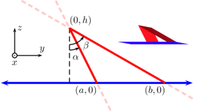
Figure 3: Weakly interacting triangular-wedge on a Dirichlet plate. The objects are of infinite extent in the $x$-direction. The weakly interacting sides of the wedge (in red) have finite length.

Observe that all irreducible two-body Casimir energies in Eq. (96) diverge due to ultra-violet contributions from the corners of the triangle where pairs of potentials overlap. More precisely, the integrand $\Delta E_{12}^{W}$ diverges when $d_{12}\sim 0$ near the vertex of the wedge. The integrand of $\Delta E_{i3}^{W}$ diverges when $z_{i}\sim 0$ near the corner with the Dirichlet plate. The irreducible three-body Casimir energy, $\Delta E_{123}^{W}$, in Eq. (99) on the other hand is finite because $\bar{d}_{12}$ never vanishes in the integration region. Substituting the potentials of Eq. (102) for the semiweak triangular waveguide in Eq. (99) and evaluating the $z$-integrals gives,

$${\cal E}(\alpha,\beta)=\frac{\Delta E_{123}^{W}}{L_{x}}\left[\frac{\lambda_{1}\lambda_{2}}{32\pi^{3}}\right]^{-1}=|\tilde{a}\,\tilde{b}|\int_{0}^{1}\int_{0}^{1}\frac{du_{1}du_{2}}{\bar{u}_{12}^{2}}\,Q\left(\frac{u_{12}^{2}}{\bar{u}_{12}^{2}}\right),$$ (103)

where we have rescaled the integration variables, $y_{1}=|a|u_{1}$ and $y_{2}=|b|u_{2}$ by the respective lengths. All distances have been expressed in units of $h$: $d_{12}=hu_{12}$ and $\bar{d}_{12}=h\bar{u}_{12}$, with

$$\bar{u}_{12}^{2} = (\tilde{a}u_{1}-\tilde{b}u_{2})^{2}+[|1-u_{1}|+|1-u_{2}|]^{2},$$ (104a)

$$u_{12}^{2} = (\tilde{a}u_{1}-\tilde{b}u_{2})^{2}+(u_{1}-u_{2})^{2}.$$ (104b)

With the function $Q(x)$ defined in Eq. (100) the three-body interaction energy of Eq. (103) is finite and can be evaluated numerically. In FIG. 4 we plot ${\cal E}(\alpha,\beta)$ as a function of the angles $\alpha$ and $\beta$. The three-body interaction energy is always positive and vanishes (and is minimized) only for $\alpha=0$, or $\beta=0$. It is minimal when the shorter side of the wedge is perpendicular to the Dirichlet plate. Wedges with angles $\beta<0<\alpha$ or $\alpha<0<\beta$ are energetically preferred over wedges with angles $\alpha,\beta>0$ or $\alpha,\beta<0$. The three-body Casimir-energy diverges only when all three sides of the triangle have a point in common, i.e. when $\alpha=\beta$, or $\alpha=-\beta=\pm\pi/2$.

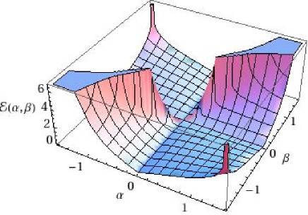
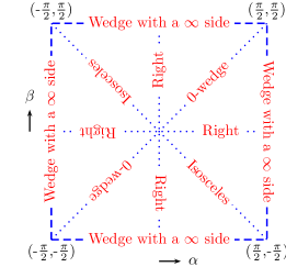
Figure 4: Casimir Landscape: ${\cal E}(\alpha,\beta)$ as a function of the opening angles $\alpha$ and $\beta$ for a weakly interacting triangular-wedge on a Dirichlet plate. The valley connecting the $\alpha>\beta$ region with the $\alpha<\beta$ region is an artifact caused by limited numerical accuracy. The valley should be replaced by a very thin and infinitely high wall describing the sharp change in energy when all surfaces overlap. On the right, the shapes of the triangles are matched to the respective regions of the $\alpha$-$\beta$ plane.

Abalo, Milton, and Kaplan, recently Abalo:2010ah investigated the dependence of the Casimir energy on the area and perimeter of triangular waveguides on which Dirichlet boundary conditions were imposed. Although only interior modes were taken into account and divergences associated with corners and single-body vacuum energies were removed ad hoc, they found that the dimensionless Casimir energy of their triangular wave guides closely follow a universal function of the dimensionless ratio ($P^{2}/A$) of the perimeter $P$ and area $A$ of the cross-section. This would imply that the Casimir energy of triangular wave guides depends on just one, rather than two, dimensionless parameters. Although we cannot expect a similar dependence, the universal behavior observed in Abalo:2010ah prompted us to also investigate the dependence of the semiweak three-body Casimir energy on the dimensionless perimeter $\tilde{p}=(P/h)$ and dimensionless area $\tilde{s}=(A/h^{2})$ of the triangular waveguide. It is also of interest to inquire for what configuration the energy of a triangular waveguide is minimized if the cross-sectional area is kept fixed. The dimensionless area $\tilde{s}$ and perimeter $\tilde{p}$ of the triangular wedge are given by,

$$\frac{A}{h^{2}} = \tilde{s}=\frac{1}{2}|\tilde{b}-\tilde{a}|,$$ (105a)

$$\frac{P}{h} = \tilde{p}=|\tilde{b}-\tilde{a}|+\sqrt{1+\tilde{a}^{2}}+\sqrt{1+\tilde{b}^{2}}.$$ (105b)

The parameter space of a triangular-wedge in this case is $\tilde{s}\geq 0$, and $\tilde{p}\geq 2\tilde{s}+2\sqrt{1+\tilde{s}^{2}}\geq\text{Max}(2,4\tilde{s})$. See FIG. 6. The inequality, $\tilde{p}>4\tilde{s}$, is a consequence of the triangle inequality.

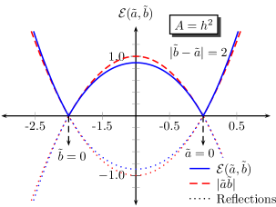
Figure 5: ${\cal E}(\tilde{a},\tilde{b})$ as a function of $\tilde{a}$ for fixed area, $A=h^{2}$. The irreducible three-body Casimir energy is minimal when the shorter side of the wedge is perpendicular to the Dirichlet plate ($\tilde{a}=0$ or $\tilde{b}=0$). The maximum in the intermediate region corresponds to the unstable equilibrium of an isosceles triangle. The dashed curves are the approximation ${\cal E}(\tilde{a},\tilde{b})\sim|\tilde{a}\tilde{b}|$ obtained by replacing the integrals in Eq. (103) with unity. The dotted curves are reflections about the ${\cal E}=0$ line.

In FIG. 5 we plot the energy as a function of $\tilde{a}$ for fixed area: $A=h^{2}$, or $|\tilde{b}-\tilde{a}|=2$, or $|\tan\beta-\tan\alpha|=2$. The three-body Casimir energy for a waveguide of given cross-sectional area is minimal when the shorter side of the wedge is perpendicular to the Dirichlet plate ($\alpha=0$ or $\beta=0~{}[\alpha=\tan^{-1}(-2)]$). In the intermediate region the energy is extremal for an isosceles triangle $(-\tilde{a}=\tilde{b}=1$) with ${\cal E}(-1,1)=0.893112\ldots$. The dashed curve in FIG. 5 represents the approximation ${\cal E}(\tilde{a},\tilde{b})\sim|\tilde{a}\tilde{b}|$ obtained by setting the dimensionless integral in Eq. (103) to 1. Remarkably, this extremely simple expression for the irreducible three-body energy is accurate to better than ten percent everywhere. We also show reflections of the curves to illustrate that the discontinuities in the slope are entirely due to the absolute value in the pre-factor $|\tilde{a}\tilde{b}|$ and the integral itself is analytic.

We rewrite the irreducible three-body Casimir energy as a function of the cross-sectional area and perimeter by inverting Eqs. (105) to obtain

$$\tilde{a} = \begin{cases}\pm\tilde{\mu}-\tilde{s},\qquad\text{if}\quad\tilde{b}>\tilde{a},\\ \pm\tilde{\mu}+\tilde{s},\qquad\text{if}\quad\tilde{b}<\tilde{a},\\ \end{cases}$$ (106a)

$$\tilde{b} = \begin{cases}\pm\tilde{\mu}+\tilde{s},\qquad\text{if}\quad\tilde{b}>\tilde{a},\\ \pm\tilde{\mu}-\tilde{s},\qquad\text{if}\quad\tilde{b}<\tilde{a},\\ \end{cases}$$ (106b)

where

$$\tilde{\mu}=\frac{1}{2\tilde{p}}\frac{(\tilde{p}-2\tilde{s})}{(\tilde{p}-4\tilde{s})}\bigg{[}\tilde{p}(\tilde{p}-4\tilde{s})\Big{\{}\tilde{p}(\tilde{p}-4\tilde{s})-4\Big{\}}\bigg{]}^{\frac{1}{2}}.$$ (107)

Substituting Eqs. (106) in Eq. (103), the three-body Casimir energy as of function of perimeter and area is

$${\cal E}(\tilde{s},\tilde{p})=|\tilde{\mu}^{2}-\,\tilde{s}^{2}|\int_{0}^{1}\int_{0}^{1}\frac{du_{1}du_{2}}{\bar{u}_{12}^{2}}\,Q\left(\frac{u_{12}^{2}}{\bar{u}_{12}^{2}}\right),$$ (108)

where the rescaled distances in terms of area and perimeter are given by

$$\bar{u}_{12}^{2} = [\tilde{\mu}(u_{1}-u_{2})+\tilde{s}(u_{1}+u_{2})]^{2}+[|1-u_{1}|+|1-u_{2}|]^{2},$$ (109a)

$$u_{12}^{2} = [\tilde{\mu}(u_{1}-u_{2})+\tilde{s}(u_{1}+u_{2})]^{2}+(u_{1}-u_{2})^{2}.$$ (109b)

In FIG. 6 the irreducible three-body contribution to the vacuum energy of a semiweak wedge is plotted as a function of dimensionless area and perimeter of the cross-section. The energy now is minimal along the curve

$$\tilde{p}=1+2\tilde{s}+\sqrt{1+4\tilde{s}^{2}}=\begin{cases}2+2\tilde{s}+{\cal O}(2\tilde{s})^{2}\qquad&2\tilde{s}<1,\\ 1+4\tilde{s}+{\cal O}\left(\frac{1}{2\tilde{s}}\right)\qquad&2\tilde{s}>1,\end{cases}$$ (110)

which corresponds to right-angled triangles. The energy diverges along the line $\tilde{p}\geq 2$, $\tilde{s}=0$, which corresponds to the two sides of the wedge coinciding ($\alpha=\beta$). In FIG. 6 the curve $\tilde{p}=1+2\tilde{s}+\sqrt{1+4\tilde{s}^{2}}$ for $s\geq 0$ corresponds to right triangles of minimal energy, and the boundary of the parameter space at $\tilde{p}=2\tilde{s}+2\sqrt{1+\tilde{s}^{2}}$ for $\tilde{s}\geq 0$ is associated with isosceles triangles.

We do not observe that ${\cal E}(\tilde{s},\tilde{p})$ is a function of $\tilde{p}^{2}/\tilde{s}$ only. The rather good approximation obtained by ignoring the dependence on the integral in Eq. (108), suggests that the energy approximately is given by

$${\cal E}(\tilde{s},\tilde{p})\sim|\tilde{\mu}^{2}-\tilde{s}^{2}|=\frac{\big{|}4(\tilde{p}-2\tilde{s})^{2}-\tilde{p}^{2}(\tilde{p}-4\tilde{s})^{2}\big{|}}{4\tilde{p}(\tilde{p}-4\tilde{s})},$$ (111)

a somewhat involved function of the perimeter and area.

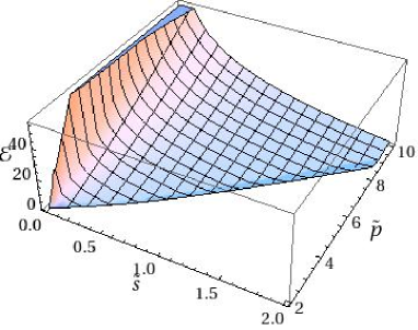
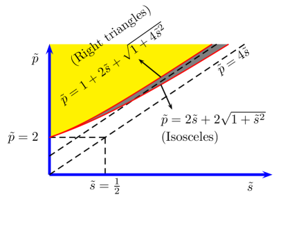
Figure 6: Irreducible three-body Casimir energy of a semiweak triangular waveguide as a function of the cross-sectional area and perimeter. This energy vanishes and is minimal along the line $\tilde{p}=1+2\tilde{s}+\sqrt{1+4\tilde{s}^{2}}$.

VIII Parabolic-wedge on a Dirichlet plate

To explicitly verify that not just corner divergences have been subtracted in the irreducible three-body contribution to the vacuum energy Schaden:2010wv , we also consider a weakly interacting parabolic-wedge on a Dirichlet plate. It is described by the potentials

$$V_{1}(y,z) = \lambda_{1}\delta(-z+\alpha(y-a)^{2})\,\theta_{1},\quad\text{with}\quad\theta_{1}\equiv\theta(y-\text{min}[0,a])\,\theta(\text{max}[0,a]-y),$$ (112a)

$$V_{2}(y,z) = \lambda_{2}\delta(-z+\beta(y-b)^{2})\,\theta_{2},\quad\text{with}\quad\theta_{2}\equiv\theta(y-\text{min}[0,b])\,\theta(\text{max}[0,b]-y),$$ (112b)

$$V_{3}(z) = \lambda_{3}\delta(z),\quad\text{with}\quad\lambda_{3}\to\infty.$$ (112c)

The parameters $\alpha$ and $\beta$ here give the foci of the parabolas and have dimensions of inverse length. The constraint $\alpha a^{2}=\beta b^{2}=h$ implies that the two parabolas intersect at $(y=0,z=h)$. See FIG. 7. As in the case of the wave guide with triangular cross-section, the base has length $|b-a|$ and the height of the wedge above the Dirichlet plate is $h$. The parameter regions are: $-\infty<a,b<\infty$, or, equivalently, $0\leq\alpha,\beta<\infty$. We measure lengths in multiples of $h$ and use parameters $(h,\tilde{a}=a/h,\tilde{b}=b/h)$ to describe it.

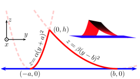
Figure 7: Weakly interacting parabolic-wedge on a Dirichlet plate.

We proceed exactly as for the triangular-wedge and find that the three-body Casimir energy of a parabolic-wedge is also given by Eq. (103), except that the distances now are given by

$$\bar{u}_{12}^{2} = (\tilde{a}u_{1}-\tilde{b}u_{2})^{2}+[(1-u_{1})^{2}+(1-u_{2})^{2}]^{2},$$ (113a)

$$u_{12}^{2} = (\tilde{a}u_{1}-\tilde{b}u_{2})^{2}+[(1-u_{1})^{2}-(1-u_{2})^{2}]^{2}.$$ (113b)

The three-body Casimir energy of a parabolic-wedge on a Dirichlet plate also is minimized when either $\tilde{a}=0,\alpha=\infty$, or $\tilde{b}=0,\beta=\infty$. Due to the constraint, $\alpha a^{2}=\beta b^{2}=h$, the shorter side of the parabolic wedge in this case degenerates to a straight line perpendicular to the Dirichlet plate. Most of the analysis of the waveguide with two sides of parabolic cross-section is the same as for a triangular one with only minor changes in interpretation. We note that the rescaled area and perimeter of the parabolic wedge are

$$\tilde{s} = \frac{1}{3}|\tilde{b}-\tilde{a}|,$$ (114a)

$$\tilde{p} = |\tilde{b}-\tilde{a}|+\frac{\tilde{a}}{2}\bigg{[}\frac{\tilde{a}^{2}}{2}\sinh^{-1}\frac{2}{\tilde{a}^{2}}+\sqrt{1+\frac{4}{\tilde{a}^{4}}}\bigg{]}+\frac{\tilde{b}}{2}\bigg{[}\frac{\tilde{b}^{2}}{2}\sinh^{-1}\frac{2}{\tilde{b}^{2}}+\sqrt{1+\frac{4}{\tilde{b}^{4}}}\bigg{]}.$$ (114b)

The three-body Casimir energy of a semiweak parabolic-wedge is shown in FIG. 8. The approximation of replacing the integral by unity is not very accurate in this case, but the overall dependence of the irreducible three-body energy of a parabolic waveguide on the parameters $\tilde{a}$ and $\tilde{b}$ is qualitatively similar to that of a triangular one.

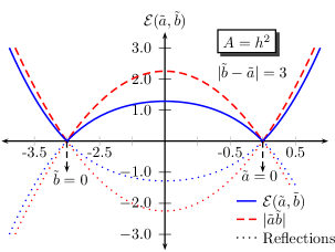
Figure 8: Irreducible three-body Casimir energy for a parabolic waveguide of given cross-sectional area. See FIG. 5 for description.

IX Discussion

In Casimir studies one generally is interested in dependence of the vacuum energy of massless quantum fields on the presence of objects whose interaction with the quantum fields is treated semiclassically, with quantum fluctuations of the fields describing the objects themselves being disregarded. This leads to an effective action with ultraviolet divergent contributions associated with geometrical properties of the objects reflected by the coefficients weyl ; Minakshisundaram:1949xg in the asymptotic expansion of the heat kernel Kac:1966xd ; Fulling:2003zx ; kirsten2002spectral . The corresponding ultra-violet divergences in the vacuum energy are proportional to the spatial volume, surface areas, curvatures, as well as number and type of corners or intersections of the objects. They depend only on local geometric properties of the system.

Fortunately, there also are non-local contributions to the vacuum energy that do not depend on the high energy description of the model and can be reliably obtained in semiclassical approximation. The best known of these is the force between disjoint classical objects due to vacuum fluctuations, first obtained for parallel metallic plates by Casimir Casimir:1948dh . It has since been shown that this force is always finite Kenneth:2006vr and that the associated finite contribution to the vacuum energy may be computed for arbitrary objects in terms of the single-body scattering matrices with Eq. (2). The investigation of generalized pistons in Schaden:PhysRevLett.102.060402 ; Schaden:PhysRevA.79.052105 suggested that one may isolate finite parts of the vacuum energy that describe the forces between objects even if these are not mutually disjoint. These ideas were formalized in Schaden:2010wv where irreducible N-body contributions to the vacuum energy were defined recursively and shown to be finite unless the N-bodies have a common intersection. For a scalar field whose interaction with N-objects are semiclassically described by positive local potentials, the irreducible contribution to the vacuum energy furthermore was found to be positive for an odd, and negative for an even, number of objects.

We have here put these general considerations on a much more practical and concrete footing and developed a formalism to extract and compute irreducible $N$-body contributions from the single-body transition matrices. Starting from Faddeev’s equations in Eq. (21), the irreducible parts of the $N$-body scattering matrix were extracted recursively. We used this formalism to compute several examples of irreducible two–and three-body Casimir energies. All our two-body results have been obtained previously, but we were able to reproduce some of them in a much simpler and direct manner. Our three-body results for irreducible Casimir energies are new. The irreducible three-body contributions to the Casimir energy of parallel semitransparent plates was obtained analytically and indeed remains finite when two of the three plates overlap. We showed explicitly how the irreducible three-body contribution precisely cancels the irreducible two-body Casimir energy of the outer plates when Dirichlet boundary conditions are imposed on the central plate–providing a raison-d’être for both, the existence, and sign, of the three-body contribution to the force. For semitransparent plates the cancellation is not complete but can be sizable.

In Section VI we analyze the irreducible three-body interaction in semiweak approximation. In this approximation we are able to compute the irreducible three-body Casimir energy for objects that are not mutually disjoint and whose irreducible two-body contributions diverge. The irreducible three-body contributions to the vacuum energy of a waveguide constructed by placing a weakly interacting triangular–or parabolic-wedge on top of a Dirichlet plate was found to be finite and computable without intermediate regularization. Our examples demonstrate that not only corner divergences, but also divergences related to curvature are subtracted by this procedure. We also explicitly verified that the irreducible three-body contribution to the vacuum energy of a massless scalar field is positive.

To develop a better understanding in a non-perturbative setting, we are currently investigating the irreducible three-body vacuum energy of a triangular waveguide formed by imposing Dirichlet boundary conditions on three intersecting infinite planes (the geometry is similar to that of FIG. 3, but with sides of infinite extent). In the limit of an extremely flat triangular cross-section, we intend to compare the numerical results with analytic calculations. We further wish to extend these methods to the physically relevant electromagnetic case. Although irreducible three-body contributions to the vacuum energy are expected to remain finite, we so far have no rigorous statements about their sign for vector fields. Interestingly, it is at least conceptually feasible to directly measure irreducible electromagnetic three-body contributions to the vacuum energy by balancing off irreducible two-body parts. We are investigating whether this is experimentally feasible.

- (1) H. B. G. Casimir, “On the attraction between two perfectly conducting plates,” Kon. Ned. Akad. Wetensch. Proc. 51, 793 (1948)
- (2) W. Lukosz, “Electromagnetic zero-point energy and radiation pressure for a rectangular cavity,” Physica 56, 109 – 120 (1971)
- (3) J. Ambjorn and S. Wolfram, “Properties of the Vacuum. 1. Mechanical and thermodynamic,” Annals of Physics 147, 1 (1983)
- (4) J. Ambjorn and S. Wolfram, “Properties of the Vacuum. 2. Electrodynamic,” Annals of Physics 147, 33 (1983)
- (5) T. H. Boyer, “Quantum electromagnetic zero point energy of a conducting spherical shell and the Casimir model for a charged particle,” Phys. Rev. 174, 1764–1774 (1968)
- (6) K. A. Milton, Jr. DeRaad, L. L., and J. S. Schwinger, “Casimir selfstress on a perfectly conducting spherical shell,” Annals of Physics 115, 388 (1978)
- (7) Jr. DeRaad, L. L. and K. A. Milton, “Casimir self-stress on a perfectly conducting cylindrical shell,” Annals of Physics 136, 229 – 242 (1981)
- (8) R. Balian and B. Duplantier, “Electromagnetic waves near perfect conductors. I. Multiple scattering expansions. Distribution of modes,” Annals of Physics 104, 300 – 335 (1977)
- (9) R. Balian and B. Duplantier, “Electromagnetic waves near perfect conductors. II. Casimir effect,” Annals of Physics 112, 165 – 208 (1978)
- (10) O. Kenneth and I. Klich, “Opposites attract: A theorem about the Casimir force,” Phys. Rev. Lett. 97, 160401 (2006), arXiv:quant-ph/0601011 [quant-ph]
- (11) T. Emig, N. Graham, R. L. Jaffe, and M. Kardar, “Casimir forces between compact objects. I. The scalar case,” Phys. Rev. D 77, 025005 (2008), arXiv:0710.3084 [cond-mat.stat-mech]
- (12) K. A. Milton and J. Wagner, “Multiple scattering methods in Casimir calculations,” J. Phys. A 41, 155402 (2008), arXiv:0712.3811 [hep-th]
- (13) L. S. Brown and M. G. Jordan, “Vacuum stress between conducting plates: An image solution,” Phys. Rev. 184, 1272–1279 (1969)
- (14) D. Deutsch and P. Candelas, “Boundary effects in quantum field theory,” Phys. Rev. D 20, 3063 (1979)
- (15) S. A. Fulling, K. A. Milton, P. Parashar, A. Romeo, K. V. Shajesh, and J. Wagner, “How does Casimir energy fall?.” Phys. Rev. D 76, 025004 (Jul 2007), arXiv:hep-th/0702091 [hep-th]
- (16) K. A. Milton, P. Parashar, K.V. Shajesh, and J. Wagner, “How does Casimir energy fall? II. Gravitational acceleration of quantum vacuum energy,” J. Phys. A 40, 10935–10943 (2007), arXiv:0705.2611 [hep-th]
- (17) K.V. Shajesh, K. A. Milton, P. Parashar, and J. A. Wagner, “How does Casimir energy fall? III. Inertial forces on vacuum energy,” J. Phys. A 41, 164058 (2008), arXiv:0711.1206 [hep-th]
- (18) I. Cavero-Pelaez, K. A. Milton, P. Parashar, and K.V. Shajesh, “Non-contact gears. I. Next-to-leading order contribution to lateral Casimir force between corrugated parallel plates,” Phys. Rev. D 78, 065018 (2008), arXiv:0805.2776 [hep-th]
- (19) I. Cavero-Pelaez, K. A. Milton, P. Parashar, and K.V. Shajesh, “Non-contact gears. II. Casimir torque between concentric corrugated cylinders for the scalar case,” Phys. Rev. D 78, 065019 (2008), arXiv:0805.2777 [hep-th]
- (20) M. F. Maghrebi, S. J. Rahi, T. Emig, N. Graham, R. L. Jaffe, and M. Kardar, “Casimir force between sharp-shaped conductors,” (2010), arXiv:1010.3223 [quant-ph]
- (21) M. F. Maghrebi, “A diagrammatic expansion of the Casimir energy in multiple reflections: Theory and applications,” Phys. Rev. D 83, 045004 (2011), arXiv:1012.1060 [quant-ph]
- (22) M. Schaden, “Finite Casimir energies of intersecting objects,” (2010), arXiv:1011.2475 [quant-ph]
- (23) E. K. Abalo, K. A. Milton, and L. Kaplan, “Casimir energies of cylinders: Universal function,” Phys. Rev. D 82, 125007 (2010), arXiv:1008.4778 [hep-th]
- (24) M. Bordag, D. Hennig, and D. Robaschik, “Vacuum energy in quantum field theory with external potentials concentrated on planes,” J. Phys. A 25, 4483–4498 (1992)
- (25) L. D. Faddeev, Mathematical aspects of the three-body problem in the quantum scattering theory (Israel Program for Scientific Translations, Jerusalem, 1965)
- (26) S. P. Merkuriev and L. D. Faddeev, Quantum scattering theory for several particle systems (Kluwer Academic, 1993)
- (27) N. C. Francis and K. M. Watson, “The elastic scattering of particles by atomic nuclei,” Phys. Rev. 92, 291–303 (Oct 1953)
- (28) K. A. Brueckner and C. A. Levinson, “Approximate reduction of the many-body problem for strongly interacting particles to a problem of self-consistent fields,” Phys. Rev. 97, 1344–1352 (Mar 1955)
- (29) P. C. Martin and J. Schwinger, “Theory of many-particle systems. I,” Phys. Rev. 115, 1342–1373 (Sep 1959)
- (30) R. D. Puff, “Ground-state properties of nuclear matter,” Annals of Physics 13, 317 – 358 (1961)
- (31) K. Kirsten, Spectral functions in mathematics and physics (Chapman & Hall/CRC Press, Boca Raton, 2002)
- (32) S. A. Fulling, Aspects of quantum field theory in curved space-time, London Mathematical Society student texts (Cambridge University Press, 1989)
- (33) M. Bordag and D. V. Vassilevich, “Nonsmooth backgrounds in quantum field theory,” Phys. Rev. D 70, 045003 (Aug 2004)
- (34) J. Wagner, K. A. Milton, and P. Parashar, “Weak coupling Casimir energies for finite plate configurations,” J. Phys. Conf. Ser. 161, 012022 (2009), arXiv:0811.2442 [hep-th]
- (35) H. Weyl, “Ueber die asymptotische Verteilung der Eigenwerte,” Nachrichten von der Gesellschaft der Wissenschaften zu Göttingen, Mathematisch-Physikalische Klasse/Zeitschriftenband (1911)/Zeitschriftenheft/Artikel/110 - 117
- (36) S. Minakshisundaram and A. Pleijel, “Some properties of the eigenfunctions of the Laplace operator on Riemannian manifolds,” Can. J. Math. 1, 242–256 (1949)
- (37) M. Kac, “Can one hear the shape of a drum?.” Am. Math. Mon. 73, 1–23 (1966)
- (38) S. A. Fulling, “Systematics of the relationship between vacuum energy calculations and heat kernel coefficients,” J. Phys. A 36, 6857–6873 (2003), arXiv:quant-ph/0302117 [quant-ph]
- (39) M. Schaden, “Dependence of the direction of the Casimir force on the shape of the boundary,” Phys. Rev. Lett. 102, 060402 (Feb 2009)
- (40) M. Schaden, “Numerical and semiclassical analysis of some generalized Casimir pistons,” Phys. Rev. A 79, 052105 (May 2009)