Effect of the Gauss-Bonnet parameter in the stability of thin-shell wormholes

Abstract

We study the stability of thin-shell wormholes in Einstein-Maxwell-Gauss-Bonnet gravity. The equation of state of the thin shell wormhole is considered first to obey a generalized Chaplygin gas and then we generalize it to an arbitrary state function which covers all known cases studied so far. In particular we study the modified Chaplygin gas and give an assessment for a general parotropic fluid. Our study is in $d-$dimensions and with numerical analysis in $d=5$ we show the effect of the GB parameter in the stability of thin-shell wormholes against the radial perturbations.

I Introduction

In an attempt to minimize the exotic matter of a traversable wormhole, Matt Visser introduced the concept of thin-shell wormhole (TSW) 1 . More precisely, in 2 two copies of the Schwarzschild spacetimes are cut and glued to make the TSW. On the other hand Brady, Louko and Poisson studied the stability of a thin shell around a black hole in 3 . In that work, using the Israel’s junction conditions 4 , the mechanical stability of a static, spherically symmetric massive thin shell has been investigated. Following this work Poisson and Visser in 5 considered the stability of the TSW against linearized perturbations around some static spherically symmetric solutions of the Einstein equations. In that paper, in particular, the form of equation of state of the matter which supports the TSW was chosen to be $p=p\left(\sigma\right)$ and following the calculation a parameter $\beta^{2}\left(\sigma\right)\equiv\frac{\partial p}{\partial\sigma}$ has been defined which plays important role for having a stable TSW. Irrespective of the form of $p\left(\sigma\right),$ it was shown that $\frac{\partial p}{\partial\sigma}$ at the static configuration which occurs at $a=a_{0}$ the equilibrium radius of the throat of the TSW appears in the final condition. The idea of TSW and its stability have been developed and generalized in many directions. Ishak and Lake, in their work 6 has continued along the previous line by adding the cosmological constant into the solution of the bulk spacetime. Eiroa and Simeone 7 developed the cylindrical TSW, Lobo studied the phantom wormholes and their stability in 8 , while TSW in dilaton gravity has been introduced in 9 . A generic, dynamic spherically symmetric thin-shell and its corresponding stability has been discussed in 10 . Chaplygin gas traversable wormholes and generalized Chaplygin gas supported spherically symmetric TSW have been discussed in 11 while higher dimensional static spherically symmetric TSW in Einstein-Maxwell theory was studied by Rahaman, Kalam and Chakraborty in 12 . Vacuum thin shell solutions in five-dimensional Lovelock gravity has been studied in SW . Extension toward the Einstein-Maxwell-Gauss-Bonnet (EMGB) was investigated in 13 and its stability and existence of TSW supported by normal matter in 14 .The non-asymptotically flat TSW in higher dimensional spherically symmetric Einstein-Yang-Mills theory has been considered in 15 and its extension to Einstein-Yang-Mills-Gauss-Bonnet is given in 16 . TSW in Hořava-Lifshitz gravity was introduced in 17 and TSW in Lovelock modified theory of gravity has been given in 18 . In 19 , rotating TSW in Kerr spacetime was found and TSW in Brans-Dicke theory and its stability were investigated in 20 . Furthermore, TSW in Dvali, Gabadadze and Porrati (DGP) theory is determined in 21 while the TSW in Einstein-nonlinear Maxwell theory has been found in 22 .

The above list is not complete and there are some other works which in some senses generalized the idea of TSW introduced in 1 ; 2 . Another form of generalization also is going on parallel to the concept of TSW which is the Israel junction conditions 4 . In 23 the generalized Darmois-Israel boundary conditions has been worked out and using it generalized junction conditions in Einstein-Gauss-Bonnet (EGB) gravity and in third order Lovelock gravity have been found in 16 ; 18 . For the whole set of Lovelock theories, the Israeal junction conditions have been generalized by Gravanisa and Willison in 24 .

Among other aspects the foremost challenging problems related to TSW 1 ; 2 ; 3 ; 4 ; 5 ; 6 ; 7 ; 8 ; 9 ; 10 ; 11 ; 12 ; 13 ; 14 ; 15 ; 16 ; 17 ; 18 ; 19 ; 20 ; 21 ; 22 are, $i$) positivity of energy density, and $ii$) stability against symmetry preserving perturbations. To overcome these problems recently there have been various attempts in EGB gravity with Maxwell and Yang-Mills sources. Specifically, with the negative Gauss-Bonnet (GB) parameter $\left(\alpha<0\right)$ we obtained stable TSW, obeying a linear equation of state, against radial perturbations 14 . By linear equation of state it is meant that the energy density $\sigma$ and surface pressure $p$ satisfy a linear relation. To respond the other challenge, however, i.e. the positivity of the energy density $\left(\sigma>0\right)$, we maintain still a cautious optimism. To be realistic, only in the case of Einstein-Yang-Mills-Gauss-Bonnet (EYMGB) theory and in a finely-tuned narrow band of parameters we were able to beat both of the above stated challenges 14 . Our stability analysis with the negative energy density was extended further to cover non-asymptotically flat (NAF) dilatonic solutions 15 .

In this paper we show that stability analysis of TSW extends to the case of a generalized Chaplygin gas (GCG) which has already been considered within the context of Einstein-Maxwell TSWs 4 . Due to the accelerated expansion of our universe a repulsive effect of a Chaplygin gas (CG) has been considered widely in recent times. By the same token therefore  it would be interesting to see how a GCG supports a TSW against radial perturbations in GB gravity. For this purpose we perturb the TSW radially and reduce the equation into a particle in a potential well problem with zero total energy. The stability amounts to the determination of the positive domain for the second derivative of the potential. We obtain plots that provides us such physical regions indicating stable wormholes. Beside the example of a GCG we consider an equation of state with quite generality. Namely, the relation between the pressure $p$ and the energy density $\sigma$ is given by the parotropic form $p=\psi\left(\sigma\right)$, for an arbitrary function $\psi\left(\sigma\right)$. The stability criteria for such a wormhole have been derived as well.

Organization of the paper is as follows. In Sec. II we introduce our formalism of TSW in EMGB theory. Stability problem of the obtained TSW supported by GCG is considered in Sec. III. In Sec. IV we generalize our equation of state further and consider cases other than the GCG. The paper ends with our Conclusion in Sec. V.

II TSW in EMGB gravity

The $d-$dimensional EMGB action without cosmological constant

$$S=\frac{1}{16\pi G}\int\sqrt{\left|g\right|}d^{d}x\left(R+\alpha\mathcal{L}_{GB}-\frac{1}{4}\mathcal{F}\right).$$ (1)

where $G$ is the $d-$dimensional Newton constant, $\mathcal{F=}F_{\mu\nu}F^{\mu\nu}$ is the Maxwell invariant and $\alpha$ is the GB parameter with Lagrangian

$$\mathcal{L}_{GB}=R^{2}-4R_{\mu\nu}R^{\mu\nu}+R_{\mu\nu\rho\sigma}R^{\mu\nu\rho\sigma}.$$ (2)

Variation of $S$ with respect to $g_{\mu\nu}$ yields the EMGB field equations,

$$G_{\mu\nu}+2\alpha H_{\mu\nu}^{\ }=T_{\mu\nu}$$ (3)

in which $H_{\mu\nu}$ and $T_{\mu\nu}$ are given by

$$H_{\mu\nu}^{\ }=2\left(-R_{\mu\text{ \ \ }}^{\ \sigma\kappa\tau}R_{\nu\sigma\kappa\tau}-2R_{\ \mu\rho\nu\sigma}^{\quad}R^{\rho\sigma}-\right.\\ \left.2R_{\mu\sigma}R_{\text{ \ }\nu}^{\sigma}+RR_{\mu\nu}^{\ }\right)-\frac{1}{2}g_{\mu\nu}^{\ }\tciLaplace_{GB},$$ (4)

$$T_{\mu\nu}=F_{\mu\alpha}F_{\nu}^{\;\alpha}-\frac{1}{4}g_{\mu\nu}F_{\alpha\beta}F^{\alpha\beta}.$$ (5)

Our static spherically symmetric metric ansatz will be

$$ds^{2}=-f\left(r\right)dt^{2}+\frac{dr^{2}}{f\left(r\right)}+r^{2}d\Omega_{d-2}^{2},$$ (6)

in which

$$d\Omega_{d-2}^{2}=d\theta_{1}^{2}+\underset{i=2}{\overset{d-2}{\mathop{\displaystyle\sum}}}\underset{j=1}{\overset{i-1}{\mathop{\displaystyle\prod}}}\sin^{2}\theta_{j}\;d\theta_{i}^{2}$$ (7)

$$0\leq\theta_{d-2}\leq 2\pi,0\leq\theta_{i}\leq\pi,1\leq i\leq d-3$$

and $f\left(r\right)$ is to be found.

Construction of the thin-shell wormhole in the static spherically symmetric spacetime follows the standard procedure used before 1 ; 2 ; 3 . In this method we consider two copies $\mathcal{M}_{1,2}$ of the spacetime

$$\mathcal{M}_{1,2}=\left\{\left.\left(t,r,\theta_{1},...,\theta_{d-2}\right)\right|r\geq a,\text{ \ }a>r_{h}\right\}$$ (8)

which are egotistically incomplete manifolds whose boundaries are given by the following timelike hypersurface

$$\Sigma_{1,2\text{ }}=\\ \left\{\left.\left(t,r,\theta_{1},...,\theta_{d-2}\right)\right|F\left(r\right)=r-a=0,\text{ \ }a>r_{h}\right\}.$$ (9)

By identifying the above hypersurfaces on $r=a$ one gets a geodesically complete manifold $\mathcal{M=M}_{1}\cup\mathcal{M}_{2}.$

We introduce the induced coordinates on the wormhole $\xi^{a}=\left(\tau,\theta_{1},\theta_{2},...\right)$ - with $\tau$ the proper time - in terms of the original bulk coordinates $x^{\gamma}=\left(t,r,\theta_{1},...,\theta_{d-2}\right).$ Further to the Israel junction conditions 4 , the generalized Darmois-Israel boundary conditions 23 , are chosen for the case of EMGB modified gravity. The latter conditions on $\Sigma$ take the form

$$2\left\langle K_{ab}-Kh_{ab}\right\rangle+\\ 4\alpha\left\langle 3J_{ab}-Jh_{ab}+2P_{acdb}K^{cd}\right\rangle=-\kappa^{2}S_{ab},$$ (10)

in which $\left\langle.\right\rangle$ stands for a jump across the hypersurface $\Sigma=\Sigma_{1\text{ }}=\Sigma_{2\text{ }}$, $h_{ab}=g_{ab}-n_{a}n_{b}$ is the induced metric on $\Sigma$ with normal vector $n_{a}$ and $S_{a}^{b}=$diag$\left(\sigma,p_{\theta_{1}},p_{\theta_{2}},...\right)$ is the energy momentum tensor on the thin-shell. Therein the extrinsic curvature $K_{ab}^{\pm}$(with trace $K$) is defined as

$$K_{ab}^{\pm}=-n_{c}^{\pm}\left(\frac{\partial^{2}x^{c}}{\partial\xi^{a}\partial\xi^{b}}+\Gamma_{mn}^{c}\frac{\partial x^{m}}{\partial\xi^{a}}\frac{\partial x^{n}}{\partial\xi^{b}}\right)_{r=a}.$$ (11)

The divergence-free part of the Riemann tensor $P_{abcd}$ and the tensor $J_{ab}$ (with trace $J$) are given also by

$$P_{abcd}=R_{abcd}+\left(R_{bc}h_{da}-R_{bd}h_{ca}\right)-\\ \left(R_{ac}h_{db}-R_{ad}h_{cb}\right)+\frac{1}{2}R\left(h_{ac}h_{db}-h_{ad}h_{cb}\right),$$ (12)

$$J_{ab}=\\ \frac{1}{3}\left[2KK_{ac}K_{b}^{c}+K_{cd}K^{cd}K_{ab}-2K_{ac}K^{cd}K_{ab}-K^{2}K_{ab}\right].$$ (13)

The black hole solution of the EMGB field equations (with $\Lambda=0$) is given by 25

$$f_{\pm}\left(r\right)=1+\frac{r^{2}}{2\tilde{\alpha}}\times\\ \left(1\pm\sqrt{1+4\tilde{\alpha}\left(\frac{2M}{8\pi r^{d-1}}-\frac{Q^{2}}{2\left(d-2\right)\left(d-3\right)r^{2\left(d-2\right)}}\right)}\right)$$ (14)

in which $\tilde{\alpha}=\left(d-3\right)\left(d-4\right)\alpha,$ $M$ is an integration constant related to the ADM mass of the BH and $Q$ is the electric charge of the BH. (We must comment that in the rest of the paper we assume $\alpha\geq 0$ and the calculations are based on the negative branch solution i.e., $f\left(r\right)=f_{-}\left(r\right)$.) The corresponding electric field $2-$form is given by

$$\mathbf{F=}\frac{Q}{r^{2\left(d-2\right)}}dt\wedge dr.$$ (15)

The components of energy momentum tensor on the thin shell are

$$\sigma=-S_{\tau}^{\tau}=\\ -\frac{\Delta\left(d-2\right)}{8\pi}\left[\frac{2}{a}-\frac{4\tilde{\alpha}}{3a^{3}}\left(\Delta^{2}-3\left(1+\dot{a}^{2}\right)\right)\right],$$ (16)

$$p=S_{\theta_{i}}^{\theta_{i}}=\frac{1}{8\pi}\left\{\frac{2\left(d-3\right)\Delta}{a}+\frac{2\ell}{\Delta}\right.-\\ \frac{4\tilde{\alpha}}{3a^{2}}\left[3\ell\Delta-\frac{3\ell}{\Delta}\left(1+\dot{a}^{2}\right)+\frac{\Delta^{3}}{a}\left(d-5\right)\right.-\\ \left.\left.\frac{6\Delta}{a}\left(a\ddot{a}+\frac{d-5}{2}\left(1+\dot{a}^{2}\right)\right)\right]\right\},$$ (17)

in which $\ell=\ddot{a}+f_{\pm}^{\prime}\left(a\right)/2$, $\Delta=\sqrt{f_{\pm}\left(a\right)+\dot{a}^{2}}$ and while a ’dot’ implies derivative with respect to the proper time $\tau$ a ’prime’ denotes differentiation with respect to the argument of the function. These expressions pertain to the static configuration if we consider $a=a_{0}=$constant and therefore

$$\sigma_{0}=-\frac{\sqrt{f_{\pm}\left(a_{0}\right)}\left(d-2\right)}{8\pi}\times\\ \left[\frac{2}{a_{0}}-\frac{4\tilde{\alpha}}{3a_{0}^{3}}\left(f_{\pm}\left(a_{0}\right)-3\right)\right],$$ (18)

$$p_{0}=\frac{\sqrt{f_{\pm}\left(a_{0}\right)}}{8\pi}\left\{\frac{2\left(d-3\right)}{a_{0}}+\frac{f_{\pm}^{\prime}\left(a_{0}\right)}{f_{\pm}\left(a_{0}\right)}-\frac{4\tilde{\alpha}}{3a_{0}^{2}}\right.\\ \left.\left[\frac{3}{2}f_{\pm}^{\prime}\left(a_{0}\right)-\frac{3f_{\pm}^{\prime}\left(a_{0}\right)}{2f_{\pm}\left(a_{0}\right)}+\left(d-5\right)\left(\frac{f_{\pm}\left(a_{0}\right)-3}{a_{0}}\right)\right]\right\}.$$ (19)

We add also that in the case of a dynamic throat the conservation equation amounts to

$$\frac{d}{d\tau}\left(\sigma a^{\left(d-2\right)}\right)+p\frac{d}{d\tau}\left(a^{\left(d-2\right)}\right)=0.$$ (20)

Figure 1: Stability region in terms of $\nu$ and radius of the throat $a_{0}$ for $d=5,$ $M=20$, $Q=1$ and various values of $\alpha.$ The stable region is denoted by $\mathrm{S.}$ The metric function is also displayed for $r$ larger than the horizon.

III Stability of the EMGBTSW supported by GCG

Our aim in the sequel is to perturb the throat of the thin-shell wormhole radially around the equilibrium radius $a_{0}.$ To do this, we assume that the equation of state is in the form of a GCG 11 , i.e.,

$$p=\left(\frac{\sigma_{0}}{\sigma}\right)^{\nu}p_{0}$$ (21)

in which $\nu\in\left(0,1\right]$ is a free parameter and $\sigma_{0}/p_{0}$ correspond to $\sigma/p$ at the equilibrium radius $a_{0}$. We plug in the latter expression into the conservation energy equation (20) to find a closed form for the dynamic tension on the thin-shell after perturbation as follows

$$\sigma\left(a\right)=\sigma_{0}\left[\left(\frac{a_{0}}{a}\right)^{\left(1+\nu\right)\left(d-2\right)}+\right.\\ \left.\frac{p_{0}}{\sigma_{0}}\left(\left(\frac{a_{0}}{a}\right)^{\left(1+\nu\right)\left(d-2\right)}-1\right)\right]^{\frac{1}{1+\nu}}.$$ (22)

Equating this with the one found in Eq. (16), one finds a particle-like equation of motion

$$\dot{a}^{2}+V\left(a\right)=0,$$ (23)

which describes the behavior of the throat after the perturbation. The intricate potential $V\left(a\right)$ satisfies

$$\sigma=-\frac{\sqrt{f_{\pm}\left(a\right)-V\left(a\right)}\left(d-2\right)}{8\pi}\times\\ \left[\frac{2}{a}-\frac{4\tilde{\alpha}}{3a^{3}}\left(f_{\pm}\left(a\right)+2V\left(a\right)-3\right)\right]$$ (24)

in which $\sigma$ is given by (22). At the static configuration at which $a=a_{0}$ one can show that $V\left(a_{0}\right)=0$ and $V^{\prime}\left(a_{0}\right)=0.$ This implies that Eq. (23) can be expanded about $a=a_{0}$ such that

$$\dot{x}^{2}+\frac{1}{2}V^{\prime\prime}\left(a_{0}\right)x^{2}=0,$$ (25)

in which $x=a-a_{0}.$ Derivative of the latter equation with respect to $\tau,$ yields

$$\ddot{x}+\frac{1}{2}V^{\prime\prime}\left(a_{0}\right)x=0,$$ (26)

which upon $V^{\prime\prime}\left(a_{0}\right)\geq 0$ admits an oscillatory motion or stability of the thin shell wormhole at $a=a_{0}$. The exact form of $V^{\prime\prime}\left(a_{0}\right)$ is given by

$$V^{\prime\prime}\left(a_{0}\right)=\frac{\mathfrak{B}_{1}\nu+\mathfrak{B}_{2}}{2a_{0}^{2}f_{0}\left[3a_{0}^{2}-2\tilde{\alpha}\left(3-f_{0}\right)\right]\left[a_{0}^{2}+2\tilde{\alpha}\left(1+f_{0}\right)\right]}$$ (27)

where

$$\mathfrak{B}_{1}=6\left[-\frac{2\tilde{\alpha}\left(d-5\right)f_{0}^{2}}{3}+\right.\\ \left.\left[\left(-f_{0}^{\prime}a_{0}+2\left(d-5\right)\right)\tilde{\alpha}+a_{0}^{2}\left(d-3\right)\right]f_{0}+\frac{f_{0}^{\prime}a_{0}\left(a_{0}^{2}+2\tilde{\alpha}\right)}{2}\right]\\ \left[4f_{0}^{2}\tilde{\alpha}+\left(-2\tilde{\alpha}f_{0}^{\prime}a_{0}-2a_{0}^{2}-12\tilde{\alpha}\right)f_{0}+f_{0}^{\prime}a_{0}\left(a_{0}^{2}+2\tilde{\alpha}\right)\right]$$ (28)

and

$$\mathfrak{B}_{2}=-16\tilde{\alpha}^{2}\left(d-5\right)f_{0}^{4}+8\tilde{\alpha}f_{0}^{3}\\ \left[\left(\tilde{\alpha}f_{0}^{\prime\prime}-18+4d\right)a_{0}^{2}+\tilde{\alpha}f_{0}^{\prime}\left(d-7\right)a_{0}+12\tilde{\alpha}\left(d-5\right)\right]\\ +\left\{\left[\left(4f_{0}^{\prime 2}-32f_{0}^{\prime\prime}\right)a_{0}^{2}-32\left(d-7\right)f_{0}^{\prime}a_{0}\right.\right.-\\ \left.144\left(d-5\right)\right]\tilde{\alpha}^{2}-16\left[f_{0}^{\prime\prime}a_{0}^{2}+\left(d-6\right)f_{0}^{\prime}a_{0}\right.+\\ \left.\left.6\left(d-4\right)-3\right]a_{0}^{2}\tilde{\alpha}-12a_{0}^{4}\tilde{\alpha}\left(d-3\right)\right\}f_{0}^{2}+2\\ \left[3a_{0}^{3}f_{0}^{\prime\prime}+3\left(d-3\right)a_{0}^{2}f_{0}^{\prime}-\right.\left.2\tilde{\alpha}\left(f_{0}^{\prime 2}-3f_{0}^{\prime\prime}\right)a_{0}+6\tilde{\alpha}f_{0}^{\prime}\left(d-7\right)\right]\\ \times\left(a_{0}^{2}+2\tilde{\alpha}\right)a_{0}f_{0}-3a_{0}^{2}f_{0}^{\prime 2}\left(a_{0}^{2}+2\tilde{\alpha}\right)^{2}.$$ (29)

Fig. 1 depicts a $5-$dimensional plot of stable region with respect to $a_{0}$ and $\nu$ with $M=20,$ $Q=1$ and variable $\tilde{\alpha}.$ The stable regions are indicated by letter $\mathrm{S.}$ As it is displayed in Fig. 1 the stability region has two parts in each case, the area in negative $\nu$ and positive $\nu.$ The former is almost for $\nu<-1$ which is not a physical state. The latter contains partly the interval $\nu\in\left(0,1\right]$ which is in our interest. We observe that by increasing $\tilde{\alpha}$ this physical stable region develops and therefore the TSW is more stable. In addition to the stable regions in Fig. 1, we plot the metric function to give an estimation of the location of the horizon for the same parameters.

Figure 2: Stability region in terms of $\eta_{0}$ and radius of the throat $a_{0}$ for CG ($\nu=1,\xi_{0}=0$), $d=5,$ $M=20$, $Q=0$ and various values of $\alpha.$ The stable region is denoted by $\mathrm{S}$ which is identified by $V^{\prime\prime}\left(a_{0}\right)>0,$ from Eqs. (27-29). The metric function is also displayed in terms of $r$. The shaded region is for $r<r_{h}$ in which $r_{h}$ is the event horizon.

Figure 3: Stability region in terms of $\eta_{0}$ and radius of the throat $a_{0}$ for CG ($\nu=1,\xi_{0}=0$), $d=5,$ $M=20$, $Q=1$ and various values of $\alpha.$ The stable region is denoted by $\mathrm{S.}$ The metric function is also displayed in terms of $r$. The shaded region is for $r<r_{h}$ in which $r_{h}$ is the event horizon.

Figure 4: Stability region in terms of $\eta_{0}$ and radius of the throat $a_{0}$ for MCG ($\nu=1,\xi_{0}=1$), $d=5,$ $M=20$, $Q=0$ and various values of $\alpha.$ The stable region is denoted by $\mathrm{S.}$ The metric function is also displayed in terms of $r$. The shaded region is for $r<r_{h}$ in which $r_{h}$ is the event horizon.

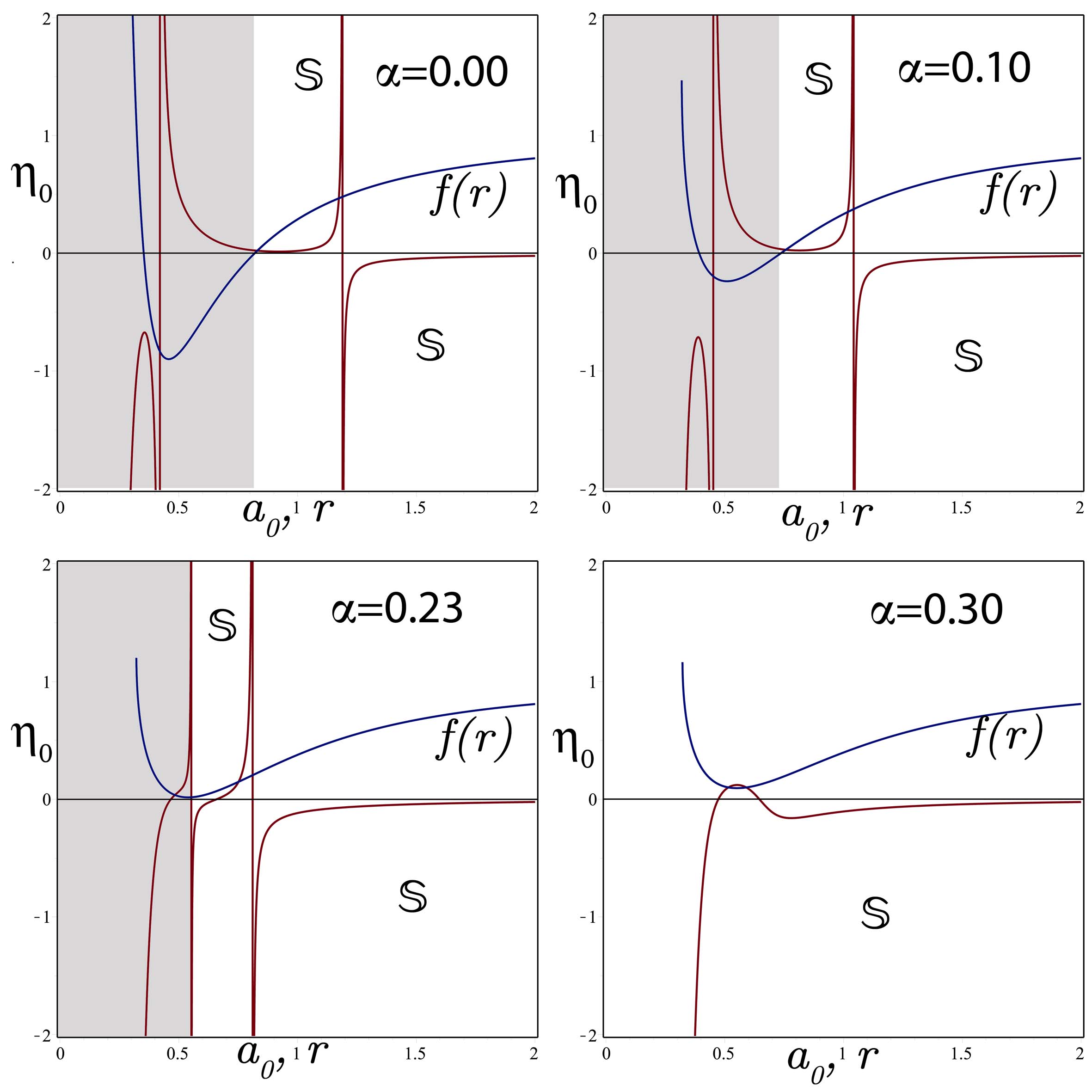
Figure 5: Stability region in terms of $\eta_{0}$ and radius of the throat $a_{0}$ for MCG ($\nu=1,\xi_{0}=1$), $d=5,$ $M=20$, $Q=1$ and various values of $\alpha.$ The stable region is denoted by $\mathrm{S.}$ The metric function is also displayed in terms of $r$. The shaded region is for $r<r_{h}$ in which $r_{h}$ is the event horizon.

IV Stability of the EMGB TSW supported by an arbitrary equation of state

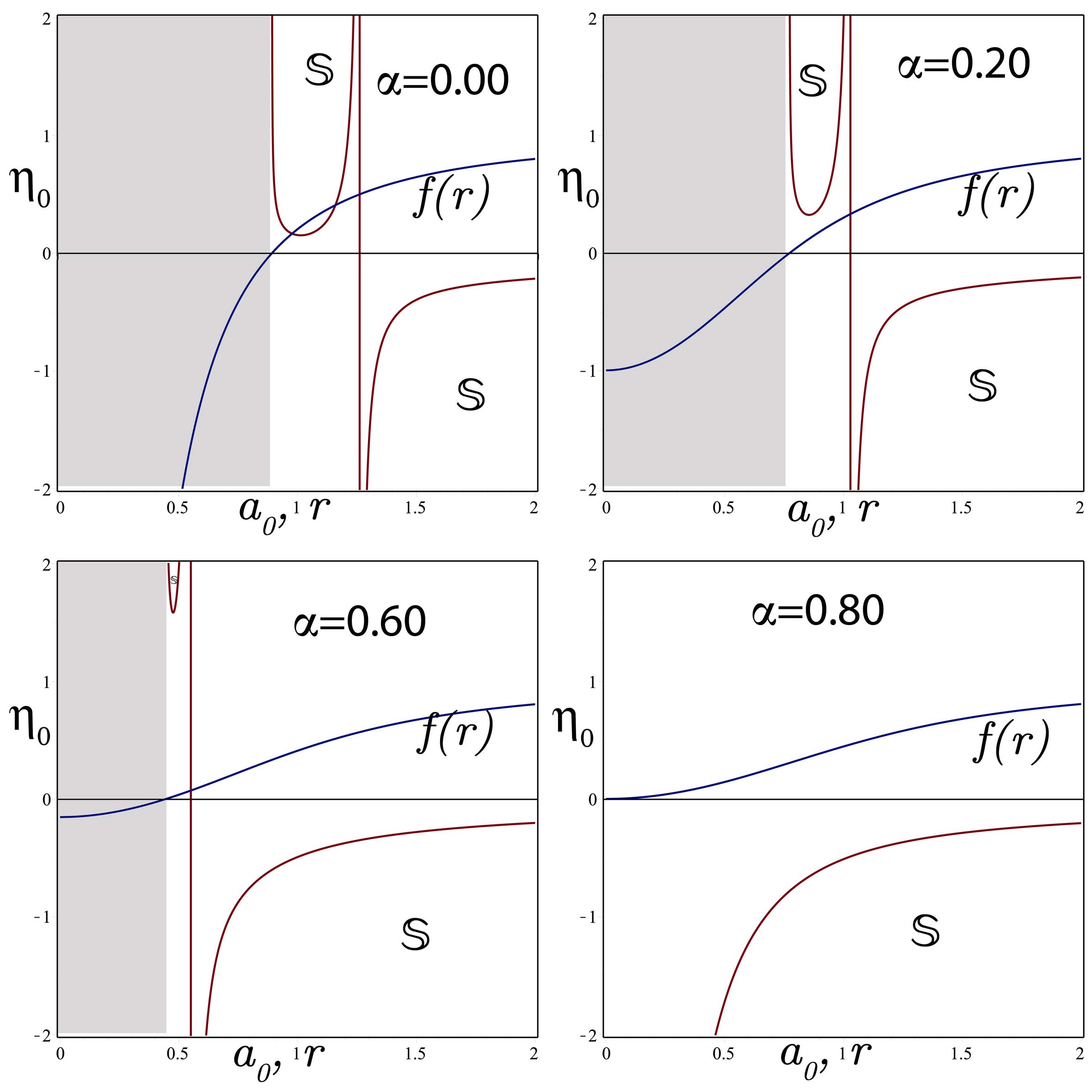
Figure 6: Stability region in terms of $\eta_{0}$ and radius of the throat $a_{0}$ for logarithmic gas (LG) for $d=5,$ $M=20$, $Q=0$ and various values of $\alpha.$ The stable region is denoted by $\mathrm{S.}$ The metric function is also displayed in terms of $r$. The shaded region is for $r<r_{h}$ in which $r_{h}$ is the event horizon.

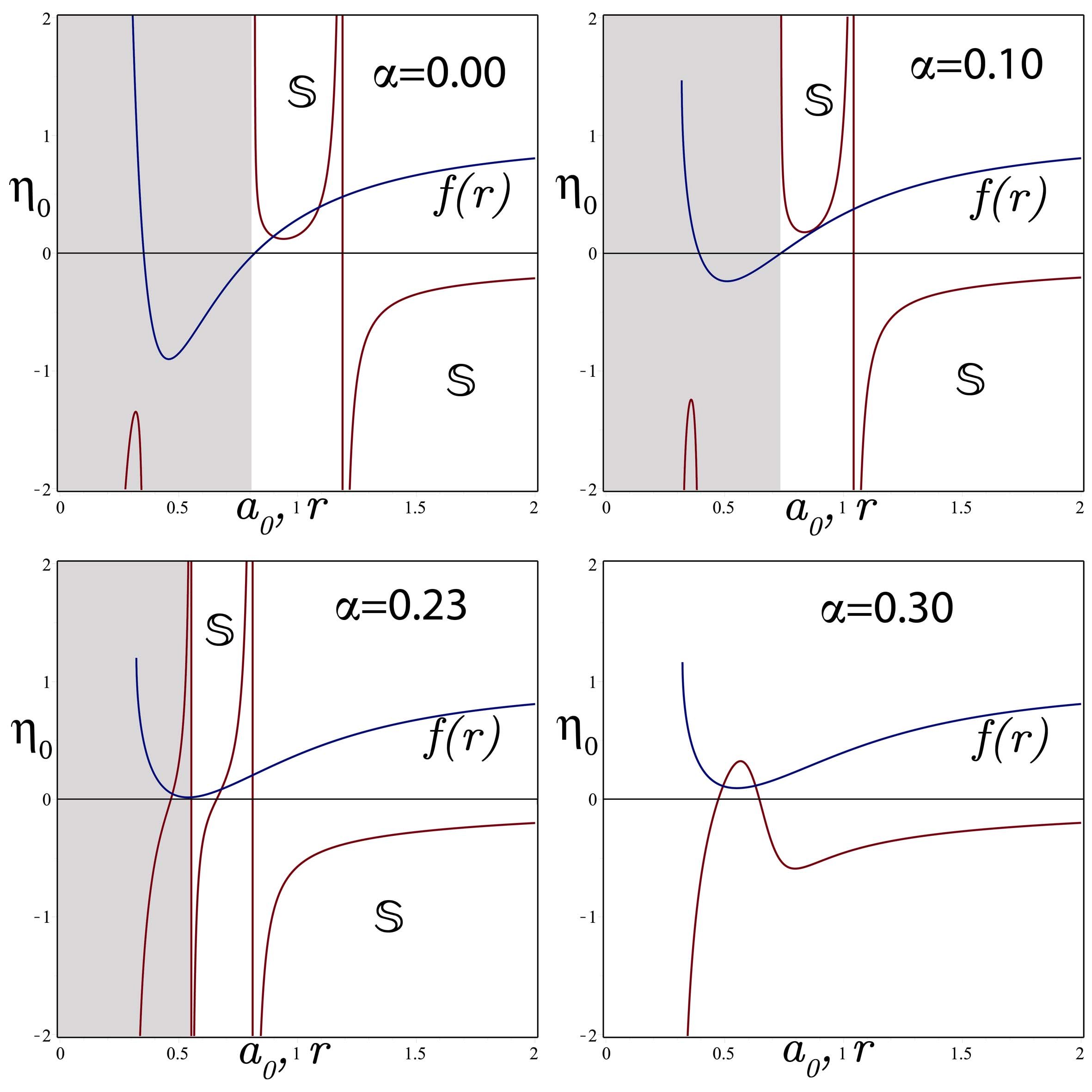
Figure 7: Stability region in terms of $\eta_{0}$ and radius of the throat $a_{0}$ for LG for $d=5,$ $M=20$, $Q=1$ and various values of $\alpha.$ The stable region is denoted by $\mathrm{S.}$ The metric function is also displayed in terms of $r$. The shaded region is for $r<r_{h}$ in which $r_{h}$ is the event horizon.

In this section we study the stability of the EMGB TSW which is supported by an arbitrary gas with the barotropic equation of state

$$p=\psi\left(\sigma\right)$$ (30)

in which $\psi\left(\sigma\right)$ is an arbitrary function of $\sigma.$ This covers naturally the polytropic equation of state $p\sim\sigma^{1+\frac{1}{n}}$ with the index $0\leq n<\infty.$ As before, we consider the static equilibrium configuration at $a=a_{0}$ where $\sigma_{0}$ and $p_{0}$ are given by (18) and (19). Furthermore, the equation of motion of the throat after the perturbation is still given by (23) where $V\left(a\right)$ satisfies the condition (24) in which $\sigma$ in the left hand side is the energy density after the perturbation. The form of $\sigma,$ explicitly, depends on the form of $p=\psi\left(\sigma\right),$ can be found by applying the energy conservation law (20) which is also equivalent with

$$\sigma^{\prime}=-\frac{d-2}{a}\left(\sigma+p\right).$$ (31)

Furthur, one has

$$\sigma^{\prime\prime}=-\frac{\left(d-2\right)}{a}p^{\prime}+\frac{\left(d-1\right)\left(d-2\right)}{a^{2}}\left(\sigma+p\right)$$ (32)

in which a prime denotes derivative with respect to $a$. Having $p^{\prime}=\psi^{\prime}\left(\sigma\right)\sigma^{\prime}$ the latter equation reads

$$\sigma^{\prime\prime}=\frac{\left(d-2\right)\left(\sigma+p\right)}{a^{2}}\left[\left(d-2\right)\psi^{\prime}\left(\sigma\right)+\left(d-1\right)\right].$$ (33)

Nevertheless, using (31) and (33), one can explicitly find the form of $V^{\prime}\left(a\right)$ and $V^{\prime\prime}\left(a\right)$ from (24) and show that at $a=a_{0}$, $V\left(a_{0}\right)$ and $V^{\prime}\left(a_{0}\right)$ vanish while

$$V^{\prime\prime}\left(a_{0}\right)=\frac{2\left(d-2\right)f_{0}\psi^{\prime}\left(\sigma_{0}\right)\mathfrak{G}_{1}+\mathfrak{G}_{2}\tilde{\alpha}+2a_{0}^{2}\mathfrak{G}_{3}}{2a_{0}^{2}f_{0}\left[a_{0}^{2}+2\tilde{\alpha}\left(1+f_{0}\right)\right]}$$ (34)

in which

$$\mathfrak{G}_{1}=4\tilde{\alpha}f_{0}^{2}-\\ \left(2\tilde{\alpha}a_{0}f_{0}^{\prime}+12\tilde{\alpha}+2a_{0}^{2}\right)f_{0}+a_{0}f_{0}^{\prime}\left(a_{0}^{2}+2\tilde{\alpha}\right),$$ (35)

$$\mathfrak{G}_{2}=8\left(d-5\right)f_{0}^{3}+\\ f_{0}^{2}\left[-4a_{0}^{2}f_{0}^{\prime\prime}-4f_{0}^{\prime}\left(d-7\right)a_{0}-24\left(d-5\right)\right]+\\ 4a_{0}\left[\left(f_{0}^{\prime\prime}-\frac{f_{0}^{\prime 2}}{2}\right)a_{0}+f_{0}^{\prime}\left(d-7\right)\right]f_{0}-2a_{0}^{2}f_{0}^{\prime 2},$$ (36)

$$\mathfrak{G}_{3}=a_{0}^{2}\left(f_{0}f_{0}^{\prime\prime}-\frac{f_{0}^{\prime 2}}{2}\right)+\left(f_{0}f_{0}^{\prime}a_{0}-2f_{0}^{2}\right)\left(d-3\right).$$ (37)

We note that $\psi^{\prime}\left(\sigma_{0}\right)\left(=\frac{p_{0}^{\prime}}{\sigma_{0}^{\prime}}\right)=\left.\frac{d\psi}{d\sigma}\right|_{\sigma=\sigma_{0}}$ while the other functions are calculated at $a=a_{0}.$ Depending on the form of $\psi$ we face different TSW. For instance setting $\frac{d\psi}{d\sigma}=\eta_{0}=$constant reduces to a linear gas supporting TSW with

$$\psi=\eta_{0}\sigma+C$$ (38)

where $C$ is a constant. Imposing $p\left(a=a_{0}\right)=p_{0}$ and $\sigma\left(a=a_{0}\right)=\sigma_{0}$ leads to $C=p_{0}-\eta_{0}\sigma_{0}$ and therefore

$$\psi=\eta_{0}\left(\sigma-\sigma_{0}\right)+p_{0}$$ (39)

which is the case studied in 26 . Another interesting case is given by $\frac{d\psi}{d\sigma}=-\frac{\eta_{0}}{\sigma^{2}}$ giving

$$\psi=\frac{\eta_{0}}{\sigma}+C$$ (40)

in which $C$ is an integration constant. Again imposing $p\left(a=a_{0}\right)=p_{0}$ and $\sigma\left(a=a_{0}\right)=\sigma_{0}$ dictates that $C=p_{0}-\frac{\eta_{0}}{\sigma_{0}}$ and therefore

$$\psi=\eta_{0}\left(\frac{1}{\sigma}-\frac{1}{\sigma_{0}}\right)+p_{0}.$$ (41)

Setting $p_{0}-\frac{\eta_{0}}{\sigma_{0}}=0$ or $\eta_{0}=p_{0}\sigma_{0}$ implies the well known CG which we have studied in the previous chapter i.e.,

$$\psi=p_{0}\frac{\sigma_{0}}{\sigma}.$$ (42)

Another important state that has been considered recently is the modified generalized Chaplygin gas MGCG obtained by setting

$$\frac{d\psi}{d\sigma} = \xi_{0}+\frac{\nu\eta_{0}}{\sigma^{\nu+1}}$$ (44)

$$\left(\xi_{0}=\text{constant}\right)$$

which implies

$$\psi=\xi_{0}\sigma-\frac{\eta_{0}}{\sigma^{\nu}}+C.$$ (45)

Applying $p\left(a=a_{0}\right)=p_{0}$ and $\sigma\left(a=a_{0}\right)=\sigma_{0}$ yields $C=p_{0}+\frac{\eta_{0}}{\sigma_{0}^{\nu}}-\xi_{0}\sigma_{0}$ and consequently

$$\psi=\xi_{0}\left(\sigma-\sigma_{0}\right)-\eta_{0}\left(\frac{1}{\sigma^{\nu}}-\frac{1}{\sigma_{0}^{\nu}}\right)+p_{0}.$$ (46)

Setting $C=0$ or $\eta_{0}=\sigma_{0}^{\nu}\left(\xi_{0}\sigma_{0}-p_{0}\right)$ simplifies the latter equation as

$$\psi=\xi_{0}\sigma-\frac{\eta_{0}}{\sigma^{\nu}}$$ (47)

which has been studied in 27 . Fig. 2 depicts the effect of GB parameter on the stability regions of the CG model of TSWH in pure GB gravity (i.e., $Q=0$). It is observed that increasing the value of the GB parameter decreases the stability areas. Fig. 2 displays stability regions as Fig. 1 but with $Q=1.$ Almost the same effect of GB parameter is seen in this case too. We note from the standard CG model that $0<\eta_{0}$ while the figures are plotted for $-2<\eta_{0}\leq 2.$ What we are referring to as the stability region should be understood in this interval.

Figs. 4 and 5 are plots of stability regions for TSW in EGB ($Q=0$) and EMGB ($Q=1$) supported by MCG ($\xi_{0}\neq 0,\eta_{0}\neq 0,\nu=1$).  Fig. 4 should be compared with Fig. 2 and Fig. 5 should be compared with Fig. 3 to see the change of the stability of the TSWH in EGB and EMGB bulk due to MCG instead of CG. We observe that effects of MCG becomes more significant for the regions of stability $r<r_{h}$ and for the cases which admits no horizon.

IV.1 A Logarithmic model of gas supporting the TSW in EMGB gravity

As one can see from Eq. (34), in $V^{\prime\prime}\left(a_{0}\right)$ only $\psi^{\prime}\left(\sigma_{0}\right)$ appears. In the case of GCG i.e. $\psi=-\frac{\eta_{0}}{\sigma^{\nu}}$ with $0<\eta_{0}$ and $0<\nu\leq 1,$ $\psi^{\prime}\left(\sigma\right)=\frac{\nu\eta_{0}}{\sigma^{\nu+1}}.$ We note that the case $\nu=0$ is excluded, for this reason separately we consider the case $\nu=0$ briefly here. When $\nu=0,$ $\psi^{\prime}\left(\sigma\right)=\frac{\eta_{0}}{\sigma}$ which implies $\psi=\eta_{0}\ln\left|\sigma\right|+C.$ In Figs. 6 and 7 we plot the stability regions of the TSW supported by the Logarithmic state equation in EGB and EMGB bulk metrics respectively.

V Conclusion

In conclusion, for a GCG obeying the equation of state $p=\left(\frac{\sigma_{0}}{\sigma}\right)^{\nu}p_{0}$, we have found stable regions within physically acceptable range of parameters in EMGB gravity. The role of GB parameter $\alpha$ in the formation of stable TSW is investigated. It is found that formation of stable regions is highly dependent on the value of $\alpha$ as depicted in our numerical plots. The energy-density, however, turns out to be negative to suppress such a TSW as a prominent candidate. Besides, a general equation of state is considered in the form $p=\psi\left(\sigma\right)$ which reproduces all known particular cases. It is found that depending on tuning of the parameters stable regions expand / shrink accordingly. Unfortunately in all cases tested one had to be satisfied with a negative energy density as the supporting agent for the TSW in EMGB theory. Finally we wish to comment that in addition to the classical role played by wormholes their possible quantum roles within the context of ”firewalls paradox” has recently been highlighted 28 . It is speculated that the emitted Hawking particles are entangled through wormholes to the inner-horizon particles of a black hole 29 . Once justified, the subject of wormholes will turn into a hot topic to transcend classical boundaries to occupy a significant role even in quantum gravity.

References

- (1) M. Visser, Phys. Rev. D 39, 3182 (1989).
- (2) M. Visser, Nucl. Phys. B 328, 203 (1989).
- (3) P. R. Brady, J. Louko and E. Poisson, Phys. Rev. D 44, 1891 (1991).
- (4) W. Israel, Nuovo Cimento 44B, 1 (1966); V. de la Cruzand W. Israel, Nuovo Cimento 51A, 774 (1967); J. E. Chase, Nuovo Cimento 67B, 136. (1970); S. K. Blau, E. I. Guendelman, and A. H. Guth, Phys. Rev. D 35, 1747 (1987); R. Balbinot and E. Poisson, Phys. Rev. D 41, 395 (1990).
- (5) E. Poisson and M. Visser, Phys. Rev. D 52, 7318 (1995).
- (6) M. Ishak and K. Lake, Phys. Rev. D 65, 044011 (2002).
- (7) E. F. Eiroa and C. Simeone, Phys. Rev. D 70, 044008 (2004); E. F. Eiroa and C. Simeone, Phys. Rev. D 81, 084022 (2010); C. Simeone, Int. Jou. of Mod. Phys. D 21, 1250015 (2012); E. F. Eiroa and C. Simeone, Phys. Rev. D 82, 084039 (2010)
- (8) F. S. Lobo, Phys. Rev. D 71, 124022 (2005) (and the references therein).
- (9) E. F. Eiroa and C. Simeone, Phys. Rev. D 71, 127501 (2005); E. F. Eiroa, Phys. Rev. D 78, 024018 (2008).
- (10) F. S. N. Lobo and P. Crawford, Class. Quantum Grav. 22, 4869 (2005); N. M. Garcia, F. S. N. Lobo and M. Visser, Phys. Rev. D 86, 044026 (2012).
- (11) F. S. N. Lobo, Phys. Rev. D 73, 064028 (2006); C. Bejarano and E. F. Eiroa, Phys. Rev. D 84, 064043 (2011); E. F. Eiroa and C. Simeone, Phys. Rev. D 76, 024021 (2007); E. F. Eiroa, Phys. Rev. D 80, 044033 (2009); M. Jamil, M. U. Farooq and M. A. Rashid, Eur. Phys. J. C 59, 907 (2009).
- (12) F. Rahaman, M. Kalam and S. Chakraborty, General Relativity and Gravitation 38, 1687 (2006).
- (13) C. Garraffo, G. Giribet, E. Gravanis and S. Willison, J. Math. Phys. 49, 042502 (2008); C. Garraffo, G. Giribet, E. Gravanis, S. Willison, arXiv:1001.3096.
- (14) M. Thibeault, C. Simeone and E. F. Eiroa, General Relativity and Gravitation 38, 1593 (2006).
- (15) M. G. Richarte and C. Simeone, Phys. Rev. D 76, 087502 (2007); D 77, 089903(E) (2008); H. Maeda and M. Nozawa, Phys. Rev. D 78, 024005 (2008); S. H. Mazharimousavi, M. Halilsoy and Z. Amirabi, Phys. Rev. D 81, 104002 (2010).
- (16) S. H. Mazharimousavi, M. Halilsoy and Z. Amirabi, Phys. Lett. A 375, 231 (2011).
- (17) S. H. Mazharimousavi, M. Halilsoy and Z. Amirabi, Classical and Quantum Gravity 28, 025004 (2011).
- (18) F. Rahaman, P. K. F. Kuhfittig, M. Kalam, A. A. Usmani and S. Ray, Classical and Quantum Gravity 28, 155021 (2011).
- (19) M. H. Dehghani and M. R. Mehdizadeh, Phys. Rev. D 85, 024024 (2012).
- (20) P. E. Kashargin and S. V. Sushkov, Gravitation and Cosmology 17, 119 (2011).
- (21) E. F. Eiroa, M. G. Richarte, C. Simeone, Phys. Lett. A 373 1 (2008); Phys. Lett. A 373, 2399 (E) (2009); X. Yue and S. Gao, Phys. Lett. A 375, 2193 (2011);’ E. F. Eiroa and C. Simeone Phys. Rev. D 82, 084039 (2010).
- (22) M. G. Richarte, Phys. Rev. D 82, 044021 (2010).
- (23) M. G. Richarte and C. Simeone, Phys. Rev. D 80, 104033 (2009); S. H. Mazharimousavi, M. Halilsoy and Z. Amirabi, Phys. Lett. A 375, 3649 (2011).
- (24) S. C. Davis, Phys. Rev. D 67, 024030 (2003).
- (25) E. Gravanis and S. Willison, J. Geom. Phys. 57, 1861 (2007).
- (26) D. G. Boulware and S. Deser, Phys. Rev. Lett. 55, 2656 (1985); M. H. Dehghani, Phys. Rev. D 67, 064017 (2003).
- (27) J. P. S. Lemos and F. S. N. Lobo, Phys. Rev. D 78, 044030 (2008).
- (28) M. Sharif and M. Azam, JCAP, 05, 025 (2013).
- (29) A. Almheiri, D. Marolf, J. Polchinski and J. Sully, JHEP. 1302, 062 (2013).
- (30) J. Maldacena, L. Susskind, ”Cool horizons for entangled black holes” arXiv:1306.0533.