Factorization Properties of Soft Graviton Amplitudes

Abstract:

We apply recently developed path integral resummation methods to perturbative quantum gravity. In particular, we provide supporting evidence that eikonal graviton amplitudes factorize into hard and soft parts, and confirm a recent hypothesis that soft gravitons are modelled by vacuum expectation values of products of certain Wilson line operators, which differ for massless and massive particles. We also investigate terms which break this factorization, and find that they are subleading with respect to the eikonal amplitude. The results may help in understanding the connections between gravity and gauge theories in more detail, as well as in studying gravitational radiation beyond the eikonal approximation.

1 Introduction

Perturbative quantum gravity has been well-studied over many decades, in the form of general relativity minimally coupled to matter particles (see [1] for a recent review), as well as alternative theories. Although the pitfalls of such an approach are well-known – chiefly that quantum general relativity contains non-renormalizable ultraviolet divergences – it is nevertheless useful for a number of reasons. Firstly, one may treat perturbative quantum gravity as an effective theory, and calculate loop corrections to gravitational observables. Secondly, it may well be the case that if a consistent quantum theory of gravity is found, it shares features with quantized general relativity. This motivates the study of features in this theory which, it may be argued, should be generically shared by alternatives. A third reason for studying gravity is that there are intriguing connections between the structure of perturbative scattering amplitudes in gravity and non-abelian gauge theories (e.g. [2, 3, 4, 5, 6, 7]). A possible application of these ideas is, for example, that of settling the question of whether $N=8$ supergravity is ultraviolet finite [8, 9, 10, 11, 12].

In light of the above remarks (and as stressed recently in [13]), an interesting property of perturbative gravity is the structure of infrared singularities. One might hope, for example, that the infrared behaviour of alternative (possibly UV finite) quantum gravity theories shares at least some of the features that underly quantum GR coupled to matter. Furthermore, the structure of IR singularities in renormalizable gauge theories is well-understood. IR divergences cancel between real and virtual contributions for sufficiently inclusive observables [14]. The singularity structure nevertheless becomes relevant in that it affects residual large contributions to the perturbative expansion of physical cross-sections which must be resummed to all orders in the coupling constant in order to obtain sensible physical predictions. Resummation is by now a highly developed subject in both abelian [15] and non-abelian gauge theories. A number of approaches exist, such as Feynman diagram methods [16, 17], Wilson line techniques [18, 19], effective field theories [20, 21, 22, 23, 24, 25], and the recently developed path integral approach of [26]. Crucial to all these approaches is the notion of factorization, namely that scattering amplitudes separate into a hard interaction, which is infrared finite, and a soft function, which contains all infrared singularities. These are generated by the emission of soft (zero momentum) gauge bosons between the external lines of the amplitude, referred to in the literature as the eikonal approximation. Such factorization properties are important both for resummation applications, and also for understanding the structure of infrared singularities to all orders [33, 34, 35, 36, 37, 38, 39, 40, 41].

The same physics also governs the infrared properties of perturbative gravity amplitudes, as first analysed in [32]. Recently, Naculich and Schnitzer have reconsidered the structure of gravitational IR divergences [13]. The main point of their paper is to argue that infrared singularities at all orders are generated by the exponentiation of the one-loop divergence i.e. that there are no subleading divergences. Their argument is based upon the assumption that gravitational amplitudes factorize in the same way that gauge theory amplitudes do, in terms of hard and soft functions. That is, the $n$-graviton scattering amplitude (adopting the notation of [13]) may be written

$$A_{n}=S_{n}\cdot H_{n},$$ (1)

where $H_{n}$ is IR-finite, and $S_{n}$ collects all IR singularities, generated by soft graviton exchange. They make the further hypothesis that, by analogy with gauge theory, the soft function can be expressed as a vacuum expectation value:

$$S_{n}=\left\langle 0\left|\prod_{i=1}^{n}\Phi_{p_{i}}(0,\infty)\right|0\right\rangle,$$ (2)

containing the Wilson line operators

$$\Phi_{p}(a,b)={\cal P}\exp\left(i\kappa\int_{a}^{b}ds\,p_{i\mu}p_{i\nu}h^{\mu\nu}(sp)\right),$$ (3)

where there is one such operator associated with each external line of the amplitude (with momentum $p_{i}$). Here $h^{\mu\nu}$ is the graviton field (we will define this more carefully in what follows), and $\kappa=32\pi G$, where $G$ is Newton’s constant. The line integral in eq. (3) is over a straight line contour, parametrized by $s$.

The aim of this paper is to examine these hypotheses within the path integral resummation framework of [26], which was developed in the context of abelian and non-abelian gauge theory. The main purpose of that paper was to address corrections to the eikonal approximation, and the result was a systematic classification of the next-to-eikonal contributions to scattering amplitudes – that is, those which occur at first subleading order in an expansion of the amplitude in the momenta of emitted gauge bosons. The results were subsequently confirmed using Feynman diagrammatic methods in [42], and have also been used to classify the structure of (non-abelian) soft gluon corrections in multiparton processes, generalising the concept of webs from two parton scattering [43, 44, 45] to the multiparton case [46, 47]. The results of [26] show that the structure of a scattering amplitude ${\cal A}$ subject to soft photon emissions has the schematic form

$${\cal A}={\cal A}_{0}\exp\left[\sum_{G^{\text{E}}}G^{\text{E}}+\sum_{G^{\text{NE}}}G^{\text{NE}}\right]\left(1+{\cal A}_{rem.}\right).$$ (4)

Here ${\cal A}_{0}$ is the hard interaction amplitude undressed by soft photons, and the exponent contains connected subdiagrams (which span the external lines) $G^{\text{E}}$ and $G^{\text{NE}}$ at eikonal and next-to-eikonal order respectively. A set of effective Feynman rules for forming these diagrams has been given in [26, 42], which generalize the well-known eikonal Feynman rules to subleading order in the momentum expansion. The term ${\cal A}_{rem.}$ in eq. (4) is also next-to-eikonal order, but does not formally exponentiate. It consists of diagrams in which eikonal photons are emitted from an external line and land inside the hard interaction. We may call these internal emission diagrams to distinguish them from the external emission diagrams which enter the exponent, and their origin makes clear that they can be thought of directly as a breaking of the factorization of the amplitude into hard and soft parts. Although internal emission contributions do not formally exponentiate, they do have an iterative structure to all orders in perturbation theory, which is fixed by gauge invariance by a result known as the Low-Burnett-Kroll theorem [57, 58] (see also [59] for a further generalization). Examples of internal and external emission contributions are shown in figure 1.

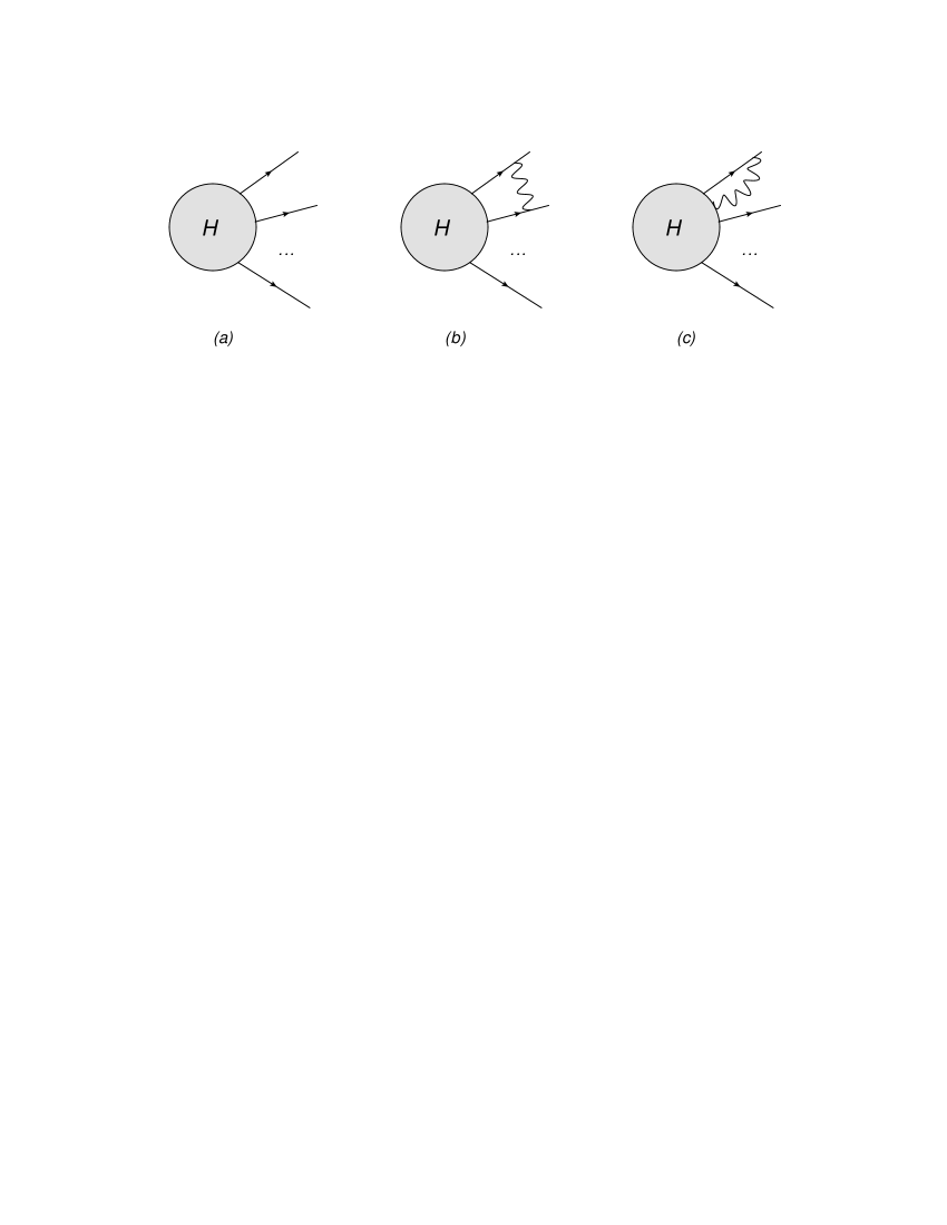
Figure 1: Examples of (a) a generic hard interaction with outgoing particles, which may emit soft gauge bosons; (b) an external emission contribution; (c) an internal emission contribution.

Although the case of abelian gauge theory is described in the preceding paragraph, a very similar structure occurs in non-Abelian theories (essentially, the sum over connected diagrams in eq. (4) is replaced by a sum over so-called webs, as described in [43, 44, 45, 48, 46, 47]). We will see in this paper that the same general structure is also observed in perturbative gravity, assuming that the infrared properties can be analysed independently of the uncertain UV completion of the theory. In particular, we will derive directly the appropriate form of the Wilson line operator which describes soft graviton emissions, as well as the appropriate gravitational generalization of Low’s theorem, which shows that internal emission contributions in gravity are subleading with respect to the eikonal approximation, as is also the case in gauge theory. These results strengthen the hypotheses made in [13], and may also shed more light on the correspondence between gauge theory and gravity.

There are also phenomenological motivations for studying corrections to eikonal gravity. The latter has been used in a variety of recent applications, in particular the study of transplanckian scattering in different gravitational theories. This has a number of potential uses, such as investigating whether different gravity theories have the same long distance behaviour [60], or even what potential collider signatures are in extra dimension scenarios [61]. The classification of corrections to the eikonal approximation, as examined in this paper, may allow further study of these and related subjects.

The structure of the paper is as follows. In section 2 we describe the path integral framework for scalar particles emitting soft gravitons, adapting the approach used for abelian gauge theory in [26], and derive the form of the Wilson line operator for soft gravitons. In section 3 we discuss how gauge invariance can be used to constrain factorization-breaking terms, and discuss how this relates to Low’s theorem [57] in QED. In section 4 we discuss our results before concluding.

2 Path integral approach to soft graviton amplitudes

In this section, we will consider the scattering amplitude for $L$ scalar particles, dressed by any number of soft gravitons. Although pure multigraviton amplitudes were considered in [13], scalar particles will be sufficient for our purposes, due to the fact that eikonal gravitons are insensitive to the spin of the particle which emits them [32].

The action for general relativity minimally coupled to a (complex) scalar field is given by

$$S_{\rm grav}=S_{\rm E.H.}[g^{\mu\nu}]+S_{\rm mat}[\phi^{*},\phi,g^{\mu\nu}],$$ (5)

here $S_{\rm E.H.}$ is the Einstein-Hilbert action (which must be suitably gauge-fixed in order to define the graviton propagator), and

$$S_{\rm mat}[\phi^{*},\phi,g^{\mu\nu}]=\int d^{d}x\sqrt{-g}\left[-g^{\mu\nu}\partial_{\mu}\phi^{*}\partial_{\nu}\phi-m^{2}\phi^{*}\phi\right],$$ (6)

in $d$ dimensions, where $g$ is the determinant of the metric tensor $g^{\mu\nu}$. Perturbation theory can then be defined after expanding the metric tensor about the flat space Minkowski metric $\eta^{\mu\nu}$. As explained in e.g. [1], there is an ambiguity in how one performs the weak field expansion. Here we adopt the approach of [62], and define

$$\tilde{g}^{\mu\nu}=\sqrt{-g}g^{\mu\nu}.$$ (7)

This introduces a Jacobian in principle in eq. (6), although this may be taken to be one in dimensional regularization [1]. We then define the graviton field $h^{\mu\nu}$ via

$$\tilde{g}^{\mu\nu}=\eta^{\mu\nu}+\kappa h^{\mu\nu},$$ (8)

where $\kappa^{2}=32\pi G$ as in [13]. Note that symmetry of the metric tensor implies $h^{\mu\nu}=h^{\nu\mu}$. One could also have chosen, of course, to expand the metric $g^{\mu\nu}$ directly. However, the choice of eq. (8) results in simpler expressions for the scalar-graviton vertices. We will return to this point later on when discussing next-to-eikonal corrections.

With the above definition for $h^{\mu\nu}$ one has [62]

$$\sqrt{-g}=1+\frac{\kappa}{d-2}h^{\alpha}_{\alpha}+\kappa^{2}\left[\frac{(h^{\alpha}_{\alpha})^{2}}{(d-2)^{2}}-\frac{h^{\alpha\beta}h_{\alpha\beta}}{d-2}\right]+{\cal O}(\kappa^{3}).$$ (9)

Furthermore, the inverse of $\tilde{g}^{\mu\nu}$ is given by [63]

$$\tilde{g}_{\mu\nu}=\eta_{\mu\nu}-\kappa h_{\mu\nu}+\kappa^{2}h_{\mu}^{\phantom{\nu}\alpha}h_{\alpha\nu}+{\cal O}(\kappa^{2}).$$ (10)

The action of eq. (6), evaluated to quadratic order in $\kappa$, is thus

$$S_{\rm mat}[\phi^{*},\phi,h^{\mu\nu}] =\int d^{d}x\left\{-\eta^{\mu\nu}\partial_{\mu}\phi^{*}\partial_{\nu}\phi-\kappa h^{\mu\nu}\partial_{\mu}\phi^{*}\partial_{\nu}\phi\right.$$

$$\left.\quad-m^{2}\phi^{*}\phi-\frac{m^{2}\kappa}{d-2}\left[h^{\alpha}_{\alpha}+\kappa\left(\frac{(h^{\alpha}_{\alpha})^{2}}{(d-2)}-h^{\alpha\beta}h_{\beta\alpha}\right)\right]\phi^{*}\phi\right\}.$$ (11)

For what follows it is useful to write this as

$$S=-\int d^{d}x\phi^{*}\hat{S}\phi,$$ (12)

where the quadratic operator $\hat{S}$ is given by

$$\hat{S} =-\eta^{\mu\nu}\partial_{\mu}\partial_{\nu}-\kappa(\partial_{\mu}h^{\mu\nu})\partial_{\nu}-\kappa h^{\mu\nu}\partial_{\mu}\partial_{\nu}+m^{2}$$

$$\quad+\frac{m^{2}\kappa}{d-2}\left[h^{\alpha}_{\alpha}+\kappa\left(\frac{(h^{\alpha}_{\alpha})^{2}}{(d-2)}-h^{\alpha\beta}h_{\beta\alpha}\right)\right]$$ (13)

(n.b. we have integrated by parts where necessary, neglecting surface terms).

The starting point of the path integral approach of [26] is to separate the gauge field (here the graviton) into hard and soft modes. That is, in the path integral which defines the quantum gravity theory, one may write

$$\int{\cal D}h^{\mu\nu}=\int{\cal D}h^{\mu\nu}_{h}{\cal D}h^{\mu\nu}_{s},$$ (14)

where $h^{\mu\nu}_{h}$ and $h^{\mu\nu}_{s}$ contain only hard and soft modes in momentum space respectively. The exact details of this definition (which may proceed e.g. by constructing an explicit hypersurface in the multigraviton momentum space which separates hard and soft parts) need not concern us, as discussed in [26] for the QED case. However, we note that this separation breaks the full gauge invariance of the gravity theory. Under a gauge transformation, the graviton behaves as

$$h^{\mu\nu}(x)\rightarrow h^{\mu\nu}(x)+\partial^{\mu}\xi^{\nu}(x)+\partial^{\nu}\xi^{\mu}(x)$$ (15)

where $x$ denotes 4-position. A general gauge function $\xi^{\mu}$ (defined in position space) will in general have both soft and hard modes in momentum space, so that gauge transformations exist which violate the separation into soft and hard modes introduced in eq. (14). However, a residual gauge invariance remains, namely that one may transform $h^{\mu\nu}$ in momentum space according to any transformation

$$h_{h,s}^{\mu\nu}(k)\rightarrow h_{h,s}^{\mu\nu}(k)+k^{\mu}\xi_{h,s}^{\nu}(k)+k^{\nu}\xi_{h,s}^{\mu}(k)$$ (16)

in which the gauge function $\xi^{\mu}_{h,s}$ contains only hard or soft modes as required. This symmetry will be sufficient to derive the structure of factorization-breaking corrections from internal emission graphs in section 3.

We now consider the Green’s function for the scattering of $L$ scalar particles which, after performing the above separation of the graviton field, may be written

$$G(p_{1}\ldots,p_{L})=\int{\cal D}h^{\mu\nu}_{s}H(x_{1},\ldots,x_{L})e^{iS_{\rm E.H.}[h^{\mu\nu}_{s}]}\prod_{j=1}^{L}\langle p_{j}|(\hat{S}-i\epsilon)^{-1}|x_{j}\rangle.$$ (17)

Here $H(x_{1},\ldots,x_{L})$ is the hard interaction, which produces scalar particles at 4-positions $\{x_{i}\}$, whose external momenta are given by $\{p_{i}\}$. This is directly analagous to the hard interaction given for the QED case in [26], except for the fact that this will now consist of a sum of Feynman diagrams involving hard graviton modes, rather than hard photon modes. There are also integrations over the positions $\{x_{i}\}$, which we do not show explicitly in eq. (17). Associated with each external line is a propagator for a scalar particle in a background soft gravitational field. According to the well-known definition of the propagator, this is given by the inverse of the quadratic operator $\hat{S}$ for the scalar field $\phi$, which includes the relevant gravitational interactions as shown in eq. (13). The propagator is sandwiched between states of given initial position and final momentum. The latter is due to the fact that Green’s functions (and, consequently, scattering amplitudes) are usually considered in momentum space. The former arises because, in what follows, we will interpret soft graviton scattering in terms of the space-time worldlines of the emitting scalars which participate in the hard interaction.

The next step is to note that the propagator factors in eq. (17) can be expressed in terms of first quantized path integrals. Such a technique arose some years ago [64, 65, 66], motivated by string theoretic approaches to field theory amplitudes [67, 68] (see also [69] for an example of worldline techniques applied in a resummation context). Here we shall quote the result as written in [26], that the propagator factors appearing in eq. (17) may be written

$$\langle p_{j}|(\hat{S}-i\epsilon)^{-1}|x_{j}\rangle =\frac{1}{2}\int_{0}^{\infty}dT\int_{x(0)=x_{j}}^{p(T)=p_{j}}{\cal D}p{\cal D}x\exp\left[\phantom{\int}-ip(T)\cdot x(T)\right.$$

$$\left.\quad+i\int_{0}^{T}dt(p\cdot\dot{x}-\hat{H}(p,x))\right],$$ (18)

where

$$\hat{H}=\frac{1}{2}\hat{S}.$$ (19)

Some explanatory comments are in order. Firstly, there is a double path integral over the position and momentum trajectories of the particle, which are parametrized in terms of a time-like variable $t$ (the upper limit of $T$ will eventually be taken to $\infty$, corresponding to the final state). The boundary conditions are that the particle must be produced at position $x_{j}$ ($x(0)=x_{j}$), and end up with final momentum $p_{j}$ ($p(T)=p_{j}$). Equation (18) arises as the solution of a Schrödinger equation for a certain evolution operator formed out of $\hat{S}$, and indeed has the recognizable Feynman path integral representation, where the second term in the exponent is the classical action formed out of the “Hamiltonian” $\hat{H}$. The first term in the exponent arises due to the fact that we are sandwiching the propagator between position and momentum states, rather than two position states. Note that the path integral over $x$ in eq. (18) has a clear physical interpretation in terms of a sum over all possible spacetime trajectories of the scalar particle whose final momentum is $p_{j}$. This will be crucial to isolating the properties of the eikonal approximation (and beyond) in what follows.

From eqs. (13) and (19), we find that the appropriate Hamiltonian operator for a scalar particle coupled to gravity is (dropping the subscript $s$ on the soft graviton field $h^{\mu\nu}_{s}$, which we do from now on)

$$\hat{H} =-\frac{1}{2}\eta^{\mu\nu}\partial_{\mu}\partial_{\nu}-\frac{\kappa}{2}(\partial_{\mu}h^{\mu\nu})\partial_{\nu}-\frac{\kappa}{2}h^{\mu\nu}\partial_{\mu}\partial_{\nu}$$

$$\quad+\frac{1}{2}m^{2}+\frac{m^{2}\kappa}{2(d-2)}\left[h^{\alpha}_{\alpha}+\kappa\left(\frac{(h^{\alpha}_{\alpha})^{2}}{(d-2)}-h^{\alpha\beta}h_{\beta\alpha}\right)\right],$$ (20)

which in momentum space ($p_{\mu}=i\partial_{\mu}$) becomes

$$\hat{H} =\frac{1}{2}(p^{2}+m^{2})+\frac{\kappa}{2}p_{\mu}p_{\nu}h^{\mu\nu}+\frac{i\kappa}{2}p_{\nu}(\partial_{\mu}h^{\mu\nu})$$

$$\quad+\frac{m^{2}\kappa}{2(d-2)}\left[h^{\alpha}_{\alpha}+\kappa\left(\frac{(h^{\alpha}_{\alpha})^{2}}{(d-2)}-h^{\alpha\beta}h_{\beta\alpha}\right)\right],$$ (21)

so that the propagator function of eq. (18) becomes

$$\langle p_{j}|(\hat{S}-i\epsilon)^{-1}|x_{j}\rangle =\frac{1}{2}\int_{0}^{\infty}dT\int_{x(0)=x_{j}}^{p(T)=p_{j}}{\cal D}p{\cal D}x\exp\left\{-ip(T)\cdot x(T)+i\int_{0}^{T}dt\left[\phantom{\int}p\cdot\dot{x}\right.\right.$$

$$\quad-\frac{1}{2}(p^{2}+m^{2})-\frac{\kappa}{2}p_{\mu}p_{\nu}h^{\mu\nu}-\frac{i\kappa}{2}p_{\nu}(\partial_{\mu}h^{\mu\nu})$$

$$\quad\left.\left.-\frac{m^{2}\kappa}{2(d-2)}\left[h^{\alpha}_{\alpha}+\kappa\left(\frac{(h^{\alpha}_{\alpha})^{2}}{(d-2)}-h^{\alpha\beta}h_{\beta\alpha}\right)\right]\right]\right\}.$$ (22)

At this point, we can recover the eikonal approximation. Recalling that this corresponds to the momentum $k$ of any emitted gravitons being completely soft ($k\rightarrow 0$), this means that the emitting scalar particles do not recoil. Thus, they follow the straight line classical trajectories

$$x(t)=x_{j}+p_{j}t.$$ (23)

Subeikonal corrections correspond to a systematic expansion about this trajectory. That is, for each external line one writes

$$x(t)\rightarrow x_{j}+p_{j}t+x(t),\quad p(t)\rightarrow p_{j}+p(t),$$ (24)

where the boundary conditions for the transformed variables are $x(0)=p(T)=0$. One then finds [26]

$$\langle p_{j}|(\hat{S}-i\epsilon)^{-1}|x_{j}\rangle =\frac{1}{2}\int_{0}^{\infty}dTe^{-ip_{j}\cdot x_{j}-\frac{1}{2}(p_{j}^{2}+m^{2})T}f(T),$$ (25)

where

$$f(T) =\int_{x(0)=0}^{p(T)=0}{\cal D}p{\cal D}x\exp\left\{i\int_{0}^{T}dt\left[p\cdot\dot{x}-\frac{1}{2}p^{2}-\frac{\kappa}{2}(p_{j\mu}+p_{\mu})(p_{j\nu}+p_{\nu})h^{\mu\nu}\right.\right.$$

$$\left.\left.\quad-\frac{i\kappa}{2}(p_{j\nu}+p_{\nu})(\partial_{\mu}h^{\mu\nu})-\frac{m^{2}\kappa}{2(d-2)}\left[h^{\alpha}_{\alpha}+\kappa\left(\frac{(h^{\alpha}_{\alpha})^{2}}{(d-2)}-h^{\alpha\beta}h_{\beta\alpha}\right)\right]\right]\right\}.$$ (26)

The path integral over $p$ is Gaussian, and may be performed explicitly. First, one writes eq. (26) as

$$f(T)=\int_{x(0)=0}^{p(T)=0}{\cal D}p{\cal D}x\exp\left[i\int_{0}^{T}dt\left(-\frac{1}{2}p_{\mu}A^{\mu\nu}p_{\nu}+B^{\mu}p_{\mu}+C\right)\right],$$ (27)

where we have defined

$$A^{\mu\nu} =\eta^{\mu\nu}+\kappa h^{\mu\nu};$$

$$B^{\mu} =\dot{x}^{\mu}-\kappa p_{j\nu}h^{\mu\nu}-\frac{i\kappa}{2}\partial_{\nu}h^{\nu\mu};$$

$$C =-\frac{\kappa}{2}p_{j\mu}p_{j\nu}h^{\mu\nu}-\frac{i\kappa}{2}p_{j\nu}\partial_{\mu}h^{\mu\nu}-\frac{m^{2}\kappa}{2(d-2)}\left[h^{\alpha}_{\alpha}+\kappa\left(\frac{(h^{\alpha}_{\alpha})^{2}}{(d-2)}-h^{\alpha\beta}h_{\beta\alpha}\right)\right],$$ (28)

and also used the fact that $h^{\mu\nu}=h^{\nu\mu}$. Using standard results for Gaussian integrals gives

$$f(T)=\int{\cal D}x\exp\left[i\int_{0}^{T}dt\left(\frac{1}{2}B^{\mu}(A^{-1})_{\mu\nu}B^{\nu}+C\right)\right],$$ (29)

where we have ignored an overall normalization constant (which is cancelled upon correctly normalising the measure for the path integral). Noting that $A^{\mu\nu}$ as defined in eq. (28) is just the metric tensor $\tilde{g}^{\mu\nu}$ of eq. (7), its inverse is simply $(A^{-1})_{\mu\nu}=\tilde{g}_{\mu\nu}$, as given in eq. (10). Then eq. (29) gives (after some tedious algebra)

$$f(T) =\int{\cal D}x\exp\left\{i\int_{0}^{T}dt\left[\frac{\dot{x}^{2}}{2}-\frac{\kappa}{2}\dot{x}^{\mu}h_{\mu\nu}\dot{x}^{\nu}-\kappa p_{j\alpha}h^{\mu\alpha}\dot{x}_{\mu}-\frac{i\kappa}{2}(\partial_{\alpha}h^{\alpha\nu})\dot{x}_{\nu}\right.\right.$$

$$\left.\left.\quad+\frac{\kappa^{2}}{2}\dot{x}^{\mu}\dot{x}^{\nu}h_{\mu}^{\phantom{\mu}\alpha}h_{\alpha\nu}+\kappa^{2}p_{j\alpha}h^{\mu\alpha}h_{\mu\nu}\dot{x}^{\nu}+\frac{i\kappa^{2}}{2}(\partial_{\beta}h^{\beta\nu})h_{\mu\nu}\dot{x}^{\mu}+\frac{\kappa^{2}}{2}p_{j\alpha}p_{j\beta}h^{\mu\alpha}h_{\mu}^{\phantom{\mu}\beta}\right.\right.$$

$$\left.\left.\quad+\frac{i\kappa^{2}}{2}p_{j\alpha}h_{\nu}^{\phantom{\nu}\alpha}(\partial_{\beta}h^{\beta\nu})-\frac{\kappa^{2}}{8}(\partial_{\alpha}h^{\alpha\mu})(\partial_{\beta}h^{\beta}_{\phantom{\beta}\mu})-\frac{\kappa}{2}p_{j\mu}p_{j\nu}h^{\mu\nu}-\frac{i\kappa}{2}p_{j\nu}\partial_{\mu}h^{\mu\nu}\right.\right.$$

$$\left.\left.\quad-\frac{m^{2}}{2}\frac{\kappa}{(d-2)}h^{\mu}_{\mu}-\frac{m^{2}\kappa^{2}}{2}\left(\frac{(h^{\alpha}_{\alpha})^{2}}{(d-2)^{2}}-\frac{h^{\alpha\beta}h_{\beta\alpha}}{d-2}\right)\right]\right\}.$$ (30)

One may relate all this back to the eikonal scattering amplitude as follows. After combining eq. (30) into eq. (25) and substituting the resulting propagator factors into the Green’s function of eq. (17), one finds (after truncating the external lines with free scalar propagators as required by the LSZ formula) that the scattering amplitude for $L$ scalar particles has the form (see the derivation in [26])

$${\cal A}(p_{1},\ldots,p_{L})=\int{\cal D}h^{\mu\nu}H(x_{1},\ldots,x_{L})e^{iS_{\rm E.H.}[h^{\mu\nu}]}\prod_{j=1}^{\infty}e^{-ip_{j}\cdot x_{j}}f_{j}(\infty).$$ (31)

That is, each external line is associated with a factor $f_{j}(\infty)$, given by eq. (30) with $T\rightarrow\infty$, which still implicitly includes a path integral over all possible trajectories of particle $j$. We will shortly analyse this result further, but first note that eq. (31) has the form of a generating functional for a quantum field theory, i.e. for the soft graviton field. The external line factors act as source terms in this theory which, as can be seen from eq. (30), generate soft graviton emission vertices localized along the external lines. The Feynman diagrams generated by eq. (31) are thus subdiagrams in the full theory, which span the external lines. Given that connected diagrams exponentiate in quantum field theory, we can immediately conclude that a large class of soft graviton corrections (namely those consisting of connected subdiagrams formed from the Feynman rules derivable from eq. (30)) exponentiate. This is a generalization of the original result in [32], which is based solely on the eikonal contributions. The argument given here for the exponentiation of soft graviton corrections based on the textbook exponentiation properties of connected diagrams in quantum field theory is essentially exactly the same as the argument used for QED in [26].

Let us now physically interpret the various terms in the external line factor of eq. (30) in more detail. First, note that the Feynman rules generated by each term cannot be immediately read off, due to the fact that for each external line the path integral over trajectories $x(t)$ has yet to be carried out. However, as shown in [26], this can be done by systematically expanding about the classical trajectory. The leading term (as already remarked above) gives the eikonal approximation, in which the particles do not recoil. The first subleading corrections give the next-to-eikonal corrections, and further corrections are next-to-next-to-eikonal etc. Put another way, an expansion about the classical trajectories of the hard emitting particles (in position space) is entirely equivalent to an expansion in the momenta of the emitted gravitons (a momentum space expansion). We may evaluate the eikonal contribution in eq. (30) by setting $x(t)=p(t)=0$, and also neglecting terms which are quadratic in $h^{\mu\nu}$ (these lead to two-graviton emission vertices, which are suppressed with respect to the eikonal limit, due to having one less eikonal denominator compared with two separate graviton emissions). One may also neglect any terms containing derivatives of the graviton field, as these (in momentum space) will be suppressed by powers of the graviton momentum. The result is

$$f^{\rm Eik.}_{j}(\infty)=\int{\cal D}x\exp\left[i\int_{0}^{\infty}dt\left(-\frac{\kappa}{2}p_{j\mu}p_{j\nu}h^{\mu\nu}-\frac{m^{2}}{2(d-2)}\eta_{\mu\nu}h^{\mu\nu}\right)\right].$$ (32)

Carrying out the path integral over $x$ gives unity assuming the appropriate normalization, and thus the eikonal approximation for the scattering amplitude is

$${\cal A}(p_{1},\ldots,p_{L}) =\int{\cal D}h^{\mu\nu}H(x_{1},\ldots,x_{L})e^{iS_{\rm E.H.}[h^{\mu\nu}]}\prod_{j=1}^{\infty}e^{-ip_{j}\cdot x_{j}}\exp\left[i\int_{0}^{\infty}dt\left(-\frac{\kappa}{2}p_{j\mu}p_{j\nu}h^{\mu\nu}\right.\right.$$

$$\left.\left.\quad-\frac{m^{2}}{2(d-2)}\eta_{\mu\nu}h^{\mu\nu}\right)\right].$$ (33)

In fact, up to next-to-eikonal corrections, one may set the initial positions of the external lines to $x_{j}=0$ [26], so that eq. (33) simplifies further to

$${\cal A}(p_{1},\ldots,p_{L}) =H(0,\ldots,0)\int{\cal D}h^{\mu\nu}e^{iS_{\rm E.H.}[h^{\mu\nu}]}\prod_{j=1}^{\infty}\exp\left[i\int_{0}^{\infty}dt\left(-\frac{\kappa}{2}p_{j\mu}p_{j\nu}h^{\mu\nu}\right.\right.$$ (34)

$$\left.\left.\quad-\frac{m^{2}}{2(d-2)}\eta_{\mu\nu}h^{\mu\nu}\right)\right],$$ (35)

where we have taken the hard interaction outside the path integral over the soft gauge field. One thus sees that the amplitude has factorized explicitly into a hard and a soft part, where the soft gravitons are described by the Wilson line factors

$$\Phi_{j}=\exp\left[i\int_{0}^{\infty}dt\left(-\frac{\kappa}{2}p_{j\mu}p_{j\nu}h^{\mu\nu}-\frac{m^{2}}{2(d-2)}\eta_{\mu\nu}h^{\mu\nu}\right)\right].$$ (36)

The generating functional for the soft graviton field theory indeed generates vacuum expectation values of these operators, as expressed in eq. (2). Let us now discuss the physics of these operators in more detail.

Firstly, the first term in the exponent in eq. (36) agrees, up to a normalization factor, with the hypothesized Wilson line operator of [13] (which dealt with pure graviton scattering, and thus massless external particles). Note, however, that the Feynman rule for the soft graviton generated by this term is derived from

$$-\frac{i\kappa}{2}\int_{0}^{\infty}dtp_{j\mu}p_{j\nu}h^{\mu\nu}(p_{j}t)=\int\frac{d^{d}k}{(2\pi)^{d}}\left(\frac{\kappa}{2}\frac{p_{\mu}p_{\nu}}{p\cdot k}h^{\mu\nu}(k)\right),$$ (37)

where $h^{\mu\nu}(k)$ is the momentum space graviton field. The momentum space eikonal Feynman rule is thus

$$\frac{\kappa}{2}\frac{p_{\mu}p_{\nu}}{p\cdot k},$$

whose normalization agrees with the result quoted in [13]. Thus, we maintain that eq. (36) is correctly normalized.

Secondly, note that there is an additional contribution in the case in which the external particles are massive, as has been considered here, which appears as the second term in the exponent of eq. (36). Wilson line operators in conventional gauge theories are the same for massless and massive particles, due to the fact that the mass does not source the gauge field. Here, however, the mass plays the role of a gravitational charge, and thus we expect such a dependence. Furthermore, such a term can be motivated on general Lorentz invariance grounds, given that the exponent of the Wilson line operator can only depend on the properties of the emitting particle. That is, the prefactor which one contracts with the graviton field can only depend upon $p^{\mu}$ and $m$, and the only two combinations having two Lorentz indices and the correct mass dimension are

$$p_{\mu}p_{\nu},\quad m^{2}\eta_{\mu\nu},$$

which indeed both occur.

Thirdly, it is interesting to note the behaviour of eq. (36) under rescalings of external line momentum. In QED, the Wilson line operator has the form

$$\Phi_{\rm QED}=\exp\left[ie\int dtp_{\mu}A^{\mu}\right],$$ (38)

where $e$ is the electromagnetic charge. This leads to the momentum-space eikonal Feynman rule

$$\frac{p_{\mu}}{p\cdot k}$$ (39)

for emission of a soft photon of momentum $k$, and this latter expression is manifestly invariant under the transformation $p\rightarrow\lambda p$, corresponding to the invariance of eq. (38) under reparametrizations of the Wilson line. By contrast, the eikonal Feynman rules generated from eq.(36) do not have this property. Rather, they can be written in the form

$$\frac{\kappa}{2}\left[p_{\mu}\left(\frac{p_{\nu}}{p\cdot k}\right)+m\left(\frac{\eta_{\mu\nu}}{2(d-2)}\frac{m}{p\cdot k}\right)\right].$$ (40)

The quantities in the round brackets are both manifestly scale invariant under rescalings of the external momentum. These are then multiplied respectively by factors of $p_{\mu}$ and $m$, namely by gravitational charges. Thus, the eikonal Feynman rules in gravity have the form of a scale-invariant (in $p$) quantity multiplied by a charge, which is exactly what one expects by analogy with abelian and non-abelian gauge theories.

The curious reader may wonder about the presence of poles in $d-2$ in the Wilson line operators. As discussed in e.g. [1], perturbation theory becomes singular in $d=2$ dimensions, owing to the fact that the Einstein-Hilbert action is then a topological invariant (i.e. there is no non-trivial dynamics). Whether or not such poles occur in the Wilson line operators is dependent on the choice of weak field approximation. If one expands the metric itself rather than absorbing $\sqrt{-g}$, the $(d-2)$ poles instead occur in the graviton propagator, such that one can never get rid of them, as expected from their physical origin.

Above, we have confirmed the factorization property of soft graviton amplitudes in the eikonal approximation, in terms of vacuum expectation values of appropriate Wilson line operators. Some comments are in order regarding the plethora of additional terms in eq. (30). As explained in [26], the path integral over $x$ in eq. (30) can be systematically expanded about the leading eikonal term. This was done for the case of abelian and non-abelian gauge theory by defining $p=\lambda n$, where $\lambda\rightarrow\infty$ isolates the eikonal term, and $n^{2}=0$ or $n^{2}=1$ for massless and massive particles respectively. The path integral could then be done perturbatively in $\lambda^{-1}$ (also taking care to expand the argument of each gauge boson field), leading to a set of next-to-eikonal Feynman rules. There were two types of next-to-eikonal vertex: those involving a single photon or gluon emission, and those involving two gauge bosons emitted from the same position on the external line. These vertices were then confirmed by an explicit diagrammatic treatment in [42].

A similar procedure is possible in the present case. Note, however, that the simple scaling $p_{j}=\lambda n_{j}$ does not solely isolate the eikonal term as $\lambda\rightarrow\infty$. Instead, eq. (30) becomes (as $\lambda\rightarrow\infty$)

$$\lim_{\lambda\rightarrow\infty}f(T) =\int{\cal D}x\exp\left\{i\int_{0}^{T}dt\left[-\frac{\kappa\lambda^{2}}{2}n_{j\mu}n_{j\nu}h^{\mu\nu}-\frac{\lambda^{2}m^{2}\kappa}{d-2}\eta_{\mu\nu}h^{\mu\nu}+\frac{\lambda^{2}\kappa^{2}}{2}n_{j\alpha}n_{j\beta}h^{\mu\alpha}h_{\mu}^{\phantom{\mu}\beta}\right.\right.$$

$$\left.\left.\quad-\frac{\lambda^{2}m^{2}\kappa^{2}}{2}\left(\frac{(h^{\alpha}_{\alpha})^{2}}{(d-2)^{2}}-\frac{h^{\alpha\beta}h_{\beta\alpha}}{d-2}\right)\right]\right\}.$$ (41)

The first two terms are the eikonal contribution of eq. (36), whereas the last two term are two-graviton vertices, which have no analogue in the case of abelian or non-abelian gauge theory. They are clearly suppressed in the eikonal limit, as such vertices have one less eikonal denominator than two separate eikonal emission vertices. The above remarks imply that the $\lambda$ scaling of [26] is not quite correct as a systematic method for expanding about the eikonal approximation, although does indeed lead to correct results for the gauge theories studied in that paper. The extra terms arise here essentially because of the weak field expansion, which allows the possibility to construct terms which are quadratic in external momenta or masses, and quadratic (or higher) in the graviton field. Such terms are absent in QED, where no weak field expansion is needed. In any case, it is straightforward to isolate next-to-eikonal contributions from power-counting, even if one does not use the $\lambda$-expansion (which amounts to little more than a convenient book-keeping device where applicable). To calculate the next-to-eikonal graviton Feynman rules, one must perform the path integral perturbatively as explained in appendix B of [26]. Here we perform this calculation in appendix A, with the result that, up to next-to-eikonal order, the external line factor of eq. (30) may be written (taking $T\rightarrow\infty$)

$$f(\infty) =\exp\left\{\int\frac{d^{d}k}{(2\pi)^{d}}h^{\mu\nu}(k)\left[\frac{\kappa}{2}\frac{p_{\mu}p_{\nu}}{p\cdot k}-\frac{\kappa}{4}\frac{p_{(\mu}k_{\nu)}}{p\cdot k}+\frac{m^{2}}{2}\frac{\kappa}{(d-2)}\frac{\eta_{\mu\nu}}{p\cdot k}+\frac{\kappa}{4}\frac{k^{2}}{(p\cdot k)^{2}}p_{\mu}p_{\nu}\right.\right.$$

$$\left.\left.+\frac{m^{2}}{4}\frac{\kappa}{d-2}\frac{k^{2}}{(p\cdot k)^{2}}\eta_{\mu\nu}\right]+\int\frac{d^{d}k}{(2\pi)^{d}}\int\frac{d^{d}l}{(2\pi)^{d}}h^{\mu\nu}(k)\,h^{\alpha\beta}(l)\left[-\frac{\kappa^{2}}{16}\left(\frac{p_{\alpha}\,p_{\beta}\,p_{(\mu}k_{\nu)}}{p\cdot k\,p\cdot(k+l)}\right.\right.\right.$$

$$\left.\left.\left.+\frac{p_{\alpha}\,p_{\beta}\,p_{(\mu}\,l_{\nu)}}{p\cdot l\,p\cdot(k+l)}+(\mu\nu\leftrightarrow\alpha\beta)\right)+\frac{\kappa^{2}}{8}\frac{p_{\mu}\,p_{\nu}\,p_{\alpha}\,p_{\beta}\,(k\cdot l)}{p\cdot k\,p\cdot l\,p\cdot(k+l)}-\frac{m^{2}\kappa^{2}}{16(d-2)}\left(\frac{\eta_{\mu\nu}\,p_{(\alpha}\,k_{\beta)}}{p\cdot k\,p\cdot(k+l)}\right.\right.\right.$$

$$\left.\left.\left.+\frac{\eta_{\mu\nu}\,p_{(\alpha}\,l_{\beta)}}{p\cdot l\,p\cdot(k+l)}+(\mu\nu\leftrightarrow\alpha\beta)\right)+\frac{m^{2}\kappa^{2}}{8(d-2)}\left(\frac{\eta_{\mu\nu}\,p_{\alpha}\,p_{\beta}\,(k\cdot l)}{p\cdot k\,p\cdot l\,p\cdot(k+l)}+(\mu\nu\leftrightarrow\alpha\beta)\right)\right.\right.$$

$$\left.\left.+\frac{m^{4}\kappa^{2}}{8(d-2)^{2}}\frac{\eta_{\mu\nu}\,\eta_{\alpha\beta}\,(k\cdot l)}{p\cdot k\,p\cdot l\,p\cdot(k+l)}+\frac{m^{2}\kappa^{2}}{4p\cdot(k+l)}\left(\frac{2\eta_{\mu\nu}\,\eta_{\alpha\beta}}{(d-2)^{2}}-\frac{1}{d-2}(\eta_{\mu\beta}\,\eta_{\nu\alpha}+\eta_{\nu\beta}\,\eta_{\mu\alpha})\right)\right]\right\}.$$ (42)

Here we have written the exponent explicitly in momentum space, where we use the argument of the graviton field to identify its Fourier-transform. From eq. (42) one can easily read off the effective Feynman rules for graviton emission up to NE order. There are eikonal and NE one-graviton vertices given by

$$\scalebox{0.6}{\includegraphics{1gE.eps}}\quad\frac{\kappa}{2}\frac{1}{p\cdot k}\left[p_{\mu}p_{\nu}+\frac{m^{2}}{d-2}\eta_{\mu\nu}\right]$$ (43)

and

$$\scalebox{0.6}{\includegraphics{1gNE.eps}}\quad\frac{\kappa}{4}\left[-\frac{p_{(\mu}k_{\nu)}}{p\cdot k}+\frac{k^{2}}{(p\cdot k)^{2}}\left(p_{\mu}\,p_{\nu}+\frac{m^{2}}{d-2}\eta_{\mu\nu}\right)\right]$$ (44)

respectively, where the eikonal result for massless particles is already well-known [32]. There is also an effective two-graviton vertex, given by

$$\left.\left.\quad-\frac{2m^{2}}{d-2}\eta_{\mu\nu}p_{\alpha}p_{\beta}(k\cdot l)+(\mu\nu\leftrightarrow\alpha\beta)\right]+2p_{\mu}\,p_{\nu}\,p_{\alpha}\,p_{\beta}(k\cdot l)+\frac{2m^{4}}{(d-2)^{2}}\eta_{\mu\nu}\eta_{\alpha\beta}(k\cdot l)\right.$$

$$\left.\quad+4m^{2}(p\cdot k)(p\cdot l)\left(\frac{2\eta_{\mu\nu}\eta_{\alpha\beta}}{(d-2)^{2}}-\frac{1}{d-2}\left(\eta_{\mu\beta}\eta_{\nu\alpha}+\eta_{\nu\beta}\eta_{\mu\alpha}\right)\right)\right\}.$$ (45)

One expects such a vertex for two reasons. Firstly, whilst successive graviton emissions are completely decoupled in the eikonal approximation, this is not expected to hold beyond the eikonal approximation, such that one expects two-graviton correlations. Secondly, there is an exact two-graviton vertex in the theory (as discussed in appendix B), which forms part of the result of eq. (45). It is useful to cross-check the above results using diagrammatic methods, as has been carried out for the case of QED and QCD in appendix B of [26]. We present such a calculation for the present case in appendix B of this paper.

The above results imply that a subset of next-to-eikonal corrections exponentiates at NE order in perturbative quantum gravity. Namely, connected external emission graphs formed from effective eikonal and NE Feynman rules, where each graph contains at most one NE vertex. Some further comments are in order regarding the results we have obtained.

To start with, one may question how useful the NE Feynman rules are in practice. Eikonal Feynman rules tell us about infrared singularities, which may be expected to be somewhat universal in alternative field theories of gravity. Next-to-eikonal corrections are non-singular, and thus potentially tell us less about generic infrared features of gravity theories. Furthermore, the fact that perturbative GR coupled to matter is not UV renormalizable suggests that an expansion in the momenta of emitted gravitons may cease to be meaningful at some point. Thus, one should be wary of taking any NE corrections too seriously. What matters in the above analysis is merely that in the soft limit, we have shown that the eikonal approximation leads to Wilson line operators as hypothesized in [13], where factorizable corrections are genuinely subleading in that they do not produce IR singularities. We have also clarified the situation when external particles have non-zero mass.

Another important point is that unlike in abelian and non-abelian gauge theory, the NE Feynman rules are not unique. They depend on the nature of the weak field approximation used to define the graviton field (e.g. whether one expands $g^{\mu\nu}$ or $\tilde{g}^{\mu\nu}$). This is not the case for the eikonal terms in four dimensions. We have verified by explicit calculation (which we do not consider worth recording here) that the Wilson line operator which occurs upon expanding $g^{\mu\nu}$ rather than $\tilde{g}^{\mu\nu}$ is

$$\Phi_{j}=\exp\left[i\int_{0}^{\infty}dt\left(-\frac{\kappa}{2}p_{j\mu}p_{j\nu}h^{\mu\nu}-\frac{m^{2}}{4}\eta_{\mu\nu}h^{\mu\nu}\right)\right].$$ (46)

Comparing this with eq. (38), we see that the two Wilson line operators are equal for $d=4$. They are also automatically equal for massless external particles. The next-to-eikonal terms, however, would differ between the two calculations, due to extra terms originating from the expansion of $\sqrt{-g}$ in the kinetic energy term for the scalar field. Such differences presumably cancel at the level of full diagrams (as the choice of weak field approximation shuffles contributions between different vertices), but it is still true that a level of ambiguity occurs in thinking about NE Feynman rules that is absent in conventional gauge theories, as a weak field expansion is not necessary in the latter.

A further comment is in order regarding the weak field approximation. In the above analysis, we have performed two expansions. Firstly, we have separated the graviton field into hard and soft modes, and used this as a basis for an expansion in the momenta of emitted gravitons. Secondly, we have expanded the graviton field itself in the gravitational coupling constant $\kappa$. In the latter expansion, we kept terms only up to ${\cal O}(\kappa^{2})$. How can we be sure that by including higher order terms, we do not induce further (next-to) eikonal corrections? To see that this is not the case, it suffices to note that any power of $\kappa$ is accompanied by a further power of the graviton field $h^{\mu\nu}$, whose Lorentz indices must be appropriately contracted with other factors of $h^{\mu\nu}$, $\dot{x}^{\mu}$, $p_{j}^{\mu}$, $p^{\mu}$ or $\partial^{\mu}$ in eq. (30). This always results in a multigraviton vertex, which is suppressed with respect to the appropriate number of eikonal 1-graviton vertices due to the fact that it lacks at least one eikonal denominator. The fact that all vertices at ${\cal O}(\kappa^{n})$ generate $n$-graviton vertices also shows that for next-to-eikonal corrections it is sufficient to expand only up to ${\cal O}(\kappa^{2})$, as we have done above. This is itself interesting, as it shows that the momentum expansion and weak field expansions are partially correlated in a well-defined sense (although there is, of course, a tower of subleading momentum terms at any given order in $\kappa$).

It follows from the above discussion that the NE Feynman rules will contain 1-graviton and 2-graviton vertices. It then follows (as for the eikonal corrections) that a large class of next-to-eikonal graviton corrections exponentiates, namely those graphs containing connected subdiagrams involving one next-to-eikonal Feynman rule. Examples are shown in figure 2.

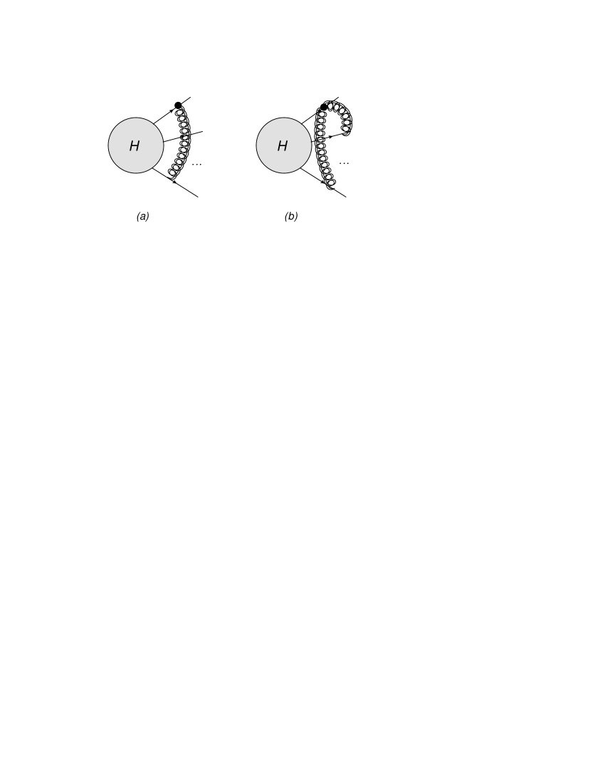
Figure 2: Example external emission graphs which exponentiate at next-to-eikonal order, where $\bullet$ represents a next-to-eikonal vertex, the doubled gluon line a graviton, and all other vertices are assumed to be eikonal.

Thus, the exponent of the scattering amplitude for $L$-particle scattering dressed by soft gravitons has the same schematic form as the QED case of eq. (4). As in that case, this is not the whole story. One may also get additional contributions from internal emission diagrams such as that shown in figure 1(c), which explicitly break the factorization of the scattering amplitude into hard and soft parts. These are known to be subleading in the soft limit in conventional gauge theories [57, 58, 59]. It is likely, but not perhaps obvious, that the same is true for gravity. This is the subject of the following section.

3 Factorization breaking terms

In the previous section, we applied the path integral resummation method of [26] to perturbative general relativity minimally coupled to a complex scalar field. We found that the amplitude factorizes into hard and soft parts, where the latter is decribed by a vacuum expectation value of Wilson line operators as in eq. (36). Explicit calculation yields diagrams formed out of eikonal Feynman rules, which then exponentiate. Corrections to the exponent are subleading, and consist of diagrams containing one next-to-eikonal Feynman rule, with all other vertices eikonal. The aim of this section is to examine what happens when this factorization is broken, and to argue that, as in QED, such corrections are next-to-eikonal, thus do not affect the structure of IR singularities.

First let us briefly recap what happens in QED. We denote by $H^{\mu}(p_{1},\ldots p_{L};k)$ the subamplitude for production of a soft photon emerging from the hard interaction $H(p_{1},\ldots p_{L})$ with momentum $k$ and with Lorentz index $\mu$. Then gauge invariance may be applied to show that $H^{\mu}$ is related to the hard interaction itself, up to next-to-eikonal order. More specifically, this relation has the following form:

$$H^{\mu}(p_{1},\ldots p_{L};k)=-\sum_{j=1}^{L}q_{j}\frac{\partial}{\partial p_{j\mu}}H(p_{1},\ldots p_{L}),$$ (47)

where $q_{j}$ is the electric charge of particle $j$. This equation tells us that factorization breaking terms are subleading with respect to the eikonal approximation. Furthermore, their structure is completely fixed up to next-to-eikonal order. Such contributions do not formally exponentiate (as do external emission graphs), but they do nevertheless have an iterative structure to all orders in perturbation theory, as given by eq. (47). This equation is an important ingredient in Low’s theorem [57, 58, 59], which relates the vertex function in gauge theory to the vertex function with an additional emission of a gauge boson.

The above result suggests that we should attempt a similar strategy in quantum gravity. That is, one may impose gauge invariance on the factorized form for the soft graviton scattering amplitude, and check that this leads to extra contributions which are suppressed with respect to the eikonal limit. As discussed in the previous section, the separation of the graviton field into hard and soft modes has broken the full gauge invariance of the theory. Nevertheless, the residual gauge symmetry under transformations of the type shown in eq. (16) will be sufficient to derive a gravitational analogue of eq. (47).

Our starting point is the factorized form of the soft graviton amplitude of eq. (33), where each external line factor is reduced to a Wilson line operator. Under a gauge transformation (eq. (15)), the Wilson operators transform as

$$f_{j}(h^{\mu\nu}+\partial^{\mu}\xi^{\nu}+\partial^{\nu}\xi^{\mu})\rightarrow f(h^{\mu\nu})e^{-i\kappa p_{j}\cdot\xi_{j}}.$$ (48)

Requiring that eq. (33) be gauge invariant then implies that the hard interaction transforms as

$$H(x_{1},\ldots x_{L};h^{\mu\nu}+\partial^{\mu}\xi^{\nu}+\partial^{\nu}\xi^{\mu})\exp\left[i\kappa\sum_{j}p_{j}\cdot\xi(x_{j})\right].$$ (49)

Expanding both sides to first order in $h^{\mu\nu}$ and $\xi^{\mu}$ gives

$$\quad H(x_{1},\ldots,x_{L})+\int d^{d}xH_{\mu\nu}(x_{1},\ldots x_{L};x)\left[h^{\mu\nu}(x)+\partial^{\mu}\xi^{\nu}(x)+\partial^{\nu}\xi^{\mu}(x)\right]$$

$$=H(x_{1},\ldots x_{L})+\int d^{d}xH_{\mu\nu}(x_{1},\ldots,x_{L};x)h^{\mu\nu}(x)$$

$$\quad+i\kappa\int d^{d}x\left[H(x_{1},\ldots x_{L})\sum_{j}p_{j\mu}\delta(x-x_{j})\right]\xi^{\mu}(x),$$ (50)

where all hard functions are evaluated with the untransformed graviton field $h^{\mu\nu}$, and $H_{\mu\nu}(x_{1},\ldots,x_{L};x)$ is the subamplitude for emission of a graviton from the hard interaction at position $x$ (this is the analogue of $H^{\mu}(x_{1},\ldots,x_{L};x)$ in the QED case, whose Fourier transform appears on the left-hand side of eq. (47)). Equation (50) simplifies to

$$\quad\int d^{d}xH_{\mu\nu}(x_{1},\ldots x_{L};x)\left[\partial^{\mu}\xi^{\nu}(x)+\partial^{\nu}\xi^{\mu}(x)\right]$$

$$=i\kappa\int d^{d}xH(x_{1},\ldots x_{L})\sum_{j}p_{j\mu}\delta(x-x_{j})\xi^{\mu}(x),$$ (51)

and integrating by parts on the left-hand side gives

$$-\int d^{d}x\xi^{\mu}\partial^{\nu}\bar{H}_{\mu\nu}=i\kappa\int d^{d}xH(x_{1},\ldots x_{L})\sum_{j}p_{j\mu}\delta(x-x_{j})\xi^{\mu}(x),$$ (52)

where $\bar{H}_{\mu\nu}=H_{\mu\nu}+H_{\nu\mu}$. Due to the fact that $\xi^{\nu}$ is arbitrary, one may write

$$-\partial^{\nu}\bar{H}_{\mu\nu}=i\kappa\sum_{j}p_{j\mu}H(x_{1},\ldots x_{L})\delta(x-x_{j}).$$ (53)

In momentum space this becomes

$$-ik^{\nu}\bar{H}_{\mu\nu}=i\kappa\sum_{j}p_{j\mu}H(p_{1},\ldots,p_{j}+k,\ldots p_{L}),$$ (54)

and expanding this to ${\cal O}(k)$ gives

$$-k^{\nu}\bar{H}_{\mu\nu}=\kappa\sum_{j}\left[p_{j\mu}+p_{j\mu}k^{\nu}\frac{\partial}{\partial p_{j}^{\nu}}\right]H(p_{1},\ldots,p_{L}).$$ (55)

The zeroth order term on the right-hand side cancels due to momentum conservation

$$\sum_{j}p_{j\mu}=0,$$ (56)

and one finally finds

$$\bar{H}_{\mu\nu}=-\kappa\sum_{j}p_{j\mu}\frac{\partial}{\partial p_{j}^{\nu}}H(p_{1},\ldots,p_{L}).$$ (57)

This is the gravitational equivalent of the QED result expressed by eq. (47). It forms part of a gravitational version of Low’s theorem, and describes the result of internal emission diagrams analagous to that shown in figure 1(c), in which a soft graviton emerges from the hard interaction and lands on an external line. Clearly such diagrams are next-to-eikonal from eq. (57). To see this, imagine starting with an external emission graph, and taking one of the soft gravitons off an external line and into the hard interaction. Such a replacement replaces an eikonal Feynman rule with the contribution of eq. (57), and the resulting diagram thus has one less eikonal denominator of form $p\cdot k$, therefore is subleading with respect to the eikonal approximation. It is worth noting that one may also derive eq. (57) from a traditional diagrammatic treatment - we present an example calculation in appendix C.

There is also an additional contribution at NE order, corresponding to the fact that the external lines do not start at the origin, but have non-zero initial 4-positions $x_{j}$, as taken into account by the factors $e^{-p_{j}\cdot x_{j}}$ in eq. (31). As in [26], one may evaluate this contribution by writing the eikonal one-graviton source term for an external line of momentum $p$ as

$$\frac{\kappa}{2}\int\frac{d^{d}k}{(2\pi)^{d}}\frac{h^{\mu\nu}}{p\cdot k}\left(p_{\mu}\,p_{\nu}+\frac{m^{2}}{d-2}\eta_{\mu\nu}\right)e^{ix\cdot k}=\frac{\kappa}{2}\int\frac{d^{d}k}{(2\pi)^{d}}\frac{h^{\mu\nu}}{p\cdot k}\left(p_{\mu}\,p_{\nu}+\frac{m^{2}}{d-2}\eta_{\mu\nu}\right)(1+ix\cdot k),$$ (58)

where we have expanded to NE order on the right-hand side. Combining the second term on the right-hand side with the rest of eq. (57), the scattering amplitude is given by

$${\cal A}(p_{1},\ldots,p_{L})=\int{\cal D}h\,e^{iS_{\rm E.H.}[h]}\left[\left(-\sum_{j=1}^{L}p_{j\mu}\frac{\partial}{\partial p_{j}^{\nu}}H(p_{1}\ldots,p_{L})\right)\int\frac{d^{d}k}{(2\pi)^{d}}h^{\mu\nu}\right.$$

$$\left.+\int dx_{1}^{d}\ldots dx_{L}^{d}H(x_{1},\ldots x_{n})\left(\sum_{j}\int\frac{d^{d}k}{(2\pi)^{d}}(ix_{j}\cdot k)\frac{h^{\mu\nu}}{p_{j}\cdot k}\left(p_{j\mu}\,p_{j\nu}+\frac{m^{2}}{d-2}\eta_{\mu\nu}\right)\right)e^{-i\sum_{j}x_{j}\cdot p_{j}}\right]$$

$$\times\prod_{j=1}^{N}f(0,p_{j};h),$$ (59)

where we have explicitly reinstated the integrals over the initial positions of the external lines, and $f(0,p_{j};h)$ is the external line factor starting at the origin for line $j$. Performing the position integrals, one obtains

$${\cal A}(p_{1},\ldots,p_{L}) =\int{\cal D}h\left\{\int\frac{d^{d}k}{(2\pi)^{d}}h^{\mu\nu}(k)\sum_{j=1}^{L}\left[-\left(p_{j\mu}\,p_{j\nu}+\frac{m^{2}}{d-2}\eta_{\mu\nu}\right)k^{\sigma}\frac{\partial}{\partial p_{j}^{\sigma}}-p_{j}^{\mu}\frac{\partial}{\partial p_{j}^{\nu}}\right]\right.$$

$$\left.\quad\times H(p_{1},\ldots,p_{L})\right\}\prod_{j=1}^{N}f(0,p_{j};h).$$ (60)

One sees that the result of the non-zero initial positions of the external lines is to add an extra NE term involving momentum derivatives of the hard interaction. A similar result occurs in QED and QCD, and it is useful to physically interpret this extra contribution. In abelian and non-abelian gauge theory, massless particles give rise to collinear as well as soft singularities, and one may write the scattering amplitude in the factorized form (analagous to eq. (1))

$${\cal A}=H\cdot S\cdot\prod_{j=1}^{L}J_{j}.$$ (61)

Here $H$ and $S$ are the hard and soft functions, where the latter collects all singularities due to the emitted gauge boson momenta satisfying $k\rightarrow 0$. Furthermore, $J_{j}$ is a jet function, and contains all singularities arising from hard emissions which are collinear to the outgoing particle of momentum $p_{j}$. Del Duca has shown [59] that in such cases there are extra contributions to the Low-Burnett-Kroll theorem due to emissions of soft gluons from inside the jet functions. This is indeed the physical meaning of the additional term in eq. (60). One would not ordinarily write jet functions in perturbative gravity, due to the fact that hard collinear singularities cancel after summing over all external particle lines and using momentum conservation [32]. However, if one is interested in the structure of next-to-eikonal corrections, there are such terms which do indeed come from emissions within jet functions, and which do not cancel after summing over parton legs (due presumably to the fact that the additional term in eq. (60) is quadratic in each external momentum). It may thus be useful to consider jet functions in gravity after all.

In this section, we have investigated the structure of terms which break the factorization of soft graviton amplitudes into hard and soft parts, and found contributions whose physical meaning is that of emission of soft gravitons from inside the hard and jet functions. All such contributions are subleading with respect to the eikonal approximation, thus verifying the factorization of graviton ampitudes at eikonal order. Furthermore, the structure of soft graviton amplitudes up to NE order has the same schematic form as in QED or QCD, namely that of eq. (4). External emission graphs (consisting of connected subdiagrams formed out of eikonal and next-to-eikonal Feynman rules) formally exponentiate, whereas internal emission graphs have an iterative structure and do not formally enter the exponent.

4 Discussion

In this paper, we have studied the recent hypothesis made in [13], that soft graviton amplitudes factorize into hard and soft functions, as do gauge theory amplitudes. Our analysis relied on path integral resummation techniques developed in the context of abelian and non-abelian gauge theory [26], which allow an efficient classification of the structure of scattering amplitudes including subleading corrections with respect to the eikonal approximation. We find that gravity amplitudes have the same schematic structure as in gauge theory, as written here in eq. (4). That is, eikonal graphs exponentiate (as already known [32]), and next-to-eikonal graphs can be separated into external and internal emission contributions. External emission graphs are connected subdiagrams formed out of effective eikonal and next-to-eikonal Feynman rules, whose form we derived in this paper. Internal emission graphs consist of soft gravitons which are emitted from inside the hard interaction, or jet functions associated with each external line. External emission graphs formally exponentiate, whereas internal emission graphs have an iterative structure to all orders in perturbation theory. Importantly, internal emission graphs are subleading with respect to the eikonal approximation.

Note that, as in the cases of QED and QCD considered in [26], one may quibble whether it is really valid to separate internal and external emission contributions as far as exponentiation is concerned, or even what is meant by next-to-eikonal exponentiation at all. After all, upon performing the exponent of the NE external emission contributions, any term involving products of two or more NE terms is NNE order or higher, such that eq. (4) is formally equivalent to

$${\cal A}={\cal A}_{0}\exp\left[\sum_{G^{\text{E}}}G^{\text{E}}\right]\left(1+\sum_{G^{\text{NE}}}G^{\text{NE}}+{\cal A}_{rem.}\right),$$ (62)

in which formula external and internal emission contributions are on the same footing. Nevertheless, it is true that the former genuinely exponentiate, whereas the latter have an iterative structure and thus must be calculated differently. Furthermore, either eq. (4) or eq. (62) allow NE contributions to be calculated to all orders in perturbation theory, even if this is really a consequence of the exponentiation of eikonal terms, as shown explicitly in eq. (62).

Aside from the structure of NE effects, an important question regarding these results is: have we formally proved the factorization of graviton amplitudes (albeit those involving only scalar external lines) into hard and soft parts? After all, the path integral technique we have used starts off by assuming that we may separate the gauge field into hard and soft modes, and that the resulting exponential structure captures all singularities. It may perhaps be prudent to regard the results we have obtained as being supporting evidence for the factorization property of amplitudes, rather than a rigorous proof. Nevertheless, it is very strong evidence, for a number of reasons. Firstly, we have analysed corrections which explicitly break the factorization property (i.e. internal emission graphs), and found these to be subleading in the momenta of the emitted gluons. We showed this using both the path integral framework, and also using diagrammatic methods (although this is essentially the same calculation, as it is gauge invariance that ultimately fixes these contributions). Secondly, we find that the structure of eikonal and next-to-eikonal contributions is exactly analagous to that of QED and QCD. This suggests that the qualitative structures one finds in the infrared limits of both gauge and gravity theories are somewhat generic. In gauge theories, the factorization property (together with the structure of the NE Feynman rules) is indeed explicitly corroborated using diagram-based methods, which gives us confidence that the same would be true for gravity. A more formal proof of the factorization of gravity amplitudes may perhaps proceed using a power-counting analysis based upon the Landau equations associated with the singularities of Feynman diagrams, as has been carried out in gauge theories (see e.g. [70] for a pedagogical review).

We are also able to confirm the hypothesis of [13] that the soft graviton part of the scattering amplitude is described by a vacuum expectation value of certain Wilson line operators, with one such operator associated with each external line. This in itself is not so surprising: in the eikonal approximation external particles do not recoil, and thus can only be changed by a phase. If this phase is to have the correct gauge transformation properties to slot into an amplitude, then some sort of Wilson line operator is inevitable. In gravity, the Wilson line operator can only depend upon $p_{\mu}\,p_{\nu}$ and $m^{2}\eta_{\mu\nu}$ due to Lorentz invariance. It is therefore reassuring to have verified that this is indeed the case. The fact that massive external particles give an additional contribution to the Wilson line operator is also expected, given that $p_{\mu}$ and $m$ play the role of charges in gravity. The exponent should consist of charges multiplying factors which are invariant under rescalings of the external momenta, which is indeed the case.

In this paper we have considered scalar particles emitting soft gravitons. One could also consider the more phenomenologically relevant examples of fermions, gauge bosons or hard gravitons emitting gravitational radiation. This should make no difference to the eikonal approximation, which is known to be insensitive to the spin of the emitting particles [32]. Beyond the eikonal approximation, and by analogy with the QED case examined in [26, 42] one expects NE corrections which are insensitive to the spin of the emitting particle, together with additional contributions which couple graviton emissions to the spin of the emitter. For fermions, this would need an appropriate curved space formulation of the second order fermion action [71], which was used in [26] to analyse fermions in the path integral approach to soft gauge boson emission.

The results presented here provide further insight into the relationships between gauge theories and perturbative quantum gravity. They may also be useful in phenomenological applications of gravitational physics e.g. extending results obtained in the eikonal approximation for transplanckian scattering [61, 60]. The investigation of such higher order effects in both gravity and gauge theories is ongoing.

Appendix A NE Feynman rules from the path integral approach

The aim of this appendix is to explicitly carry out the path integral of eq. (30), perturbatively about the classical trajectory. We will keep terms up to and including next-to-eikonal corrections, for which a weak field expansion to ${\cal O}(\kappa^{2})$ is sufficient. The calculation closely follows that of the QED case in appendix B of [26].

We begin by noting that the first term in the exponent of eq. (30) defines the quadratic operator (after taking $T\rightarrow\infty$)

$$i\int_{0}^{\infty}dt\frac{\dot{x}^{2}}{2}\equiv\int_{0}^{\infty}dtx_{\mu}\left(-\frac{i}{2}\eta^{\mu\nu}\frac{d^{2}}{dt^{2}}\right)x_{\nu},$$ (63)

where we have integrated by parts on the right-hand side. The propagator for the $x_{\mu}$ coordinate is given by the inverse of this operator, which is [26]

$$G(t,t^{\prime})=i\min(t,t^{\prime})\eta_{\mu\nu}.$$ (64)

This in turn leads to the following correlators, which we will need in what follows:

$$\langle x_{\mu}(t)x_{\nu}(t^{\prime})\rangle=G(t,t^{\prime})=i\min(t,t^{\prime})\eta_{\mu\nu}$$

$$\langle\dot{x}_{\mu}(t)x_{\nu}(t^{\prime})\rangle=\frac{\partial G(t,t^{\prime})}{\partial t}=i\Theta(t^{\prime}-t)\eta_{\mu\nu}$$ (65)

$$\langle\dot{x}_{\mu}(t)\dot{x}_{\nu}(t^{\prime})\rangle=\frac{\partial^{2}G(t,t^{\prime})}{\partial t\partial t^{\prime}}=i\delta(t-t^{\prime})\eta_{\mu\nu},$$

where $\Theta(t-t^{\prime})$ is the Heaviside function. Note that the second and third correlators vanish at equal times ($t=t^{\prime}$). To see this, one may use finite difference formulae consistent with the space-time discretization assumed in the path integral derivation of [26] to write

$$\langle x_{\mu}(t)\dot{x}_{\nu}(t)\rangle=\lim_{\epsilon\rightarrow 0^{+}}\frac{\langle x_{\mu}(t)[x_{\nu}(t+\epsilon)-x_{\nu}(t)]\rangle}{\epsilon}=0,$$ (66)

where we have used the first correlator of eq. (65) for the final equality. Likewise, one may write

$$\langle\dot{x}_{\mu}(t)\dot{x}_{\nu}(t)\rangle=-\langle x_{\mu}(t)\ddot{x}_{\nu}(t)\rangle$$ (67)

(using integration by parts), which gives

$$\langle x_{\mu}(t)\ddot{x}_{\nu}(t)\rangle=-\lim_{\epsilon\rightarrow 0^{+}}\frac{\langle x_{\mu}(t)[x_{\nu}(t+2\epsilon)-x_{\nu}(t+\epsilon)+x_{\nu}(t)]\rangle}{\epsilon^{2}}=0.$$ (68)

We now consider the external line factor of eq. (30), where for brevity in what follows we write $p_{j}\rightarrow p$. Furthermore, we may use the symmetry of $h^{\mu\nu}$ to rewrite eq. (30) in the $T\rightarrow\infty$ limit as

$$f(\infty) =\int{\cal D}x\,\exp\left\{i\int_{0}^{\infty}dt\left[\frac{\dot{x}^{2}}{2}-\frac{\kappa}{2}p_{(\nu}\dot{x}_{\mu)}h^{\mu\nu}-\frac{i\kappa}{2}(\partial_{\mu}h^{\mu\nu})\dot{x}_{\nu}+\frac{\kappa^{2}}{8}\left(p_{\nu}\,p_{\beta}\,\eta_{\alpha\mu}+p_{\mu}\,p_{\beta}\,\eta_{\alpha\nu}\right.\right.\right.$$

$$\left.\left.\left.+p_{\nu}\,p_{\alpha}\,\eta_{\beta\mu}+p_{\mu}\,p_{\alpha}\,\eta_{\beta\nu}\right)h^{\mu\nu}h^{\alpha\beta}-\frac{\kappa}{2}p_{\mu}\,p_{\nu}h^{\mu\nu}-\frac{i\kappa}{4}p_{(\nu}\partial_{\mu)}h^{\mu\nu}-\frac{m^{2}}{2}\frac{\kappa}{d-2}\eta_{\mu\nu}h^{\mu\nu}\right.\right.$$

$$\left.\left.+\frac{i\kappa^{2}}{4}p_{(\nu}\eta_{\mu)\beta}h^{\mu\nu}(\partial_{\alpha}h^{\alpha\beta})-\frac{m^{2}\kappa^{2}}{2}\left(\frac{\eta_{\mu\nu}\,\eta_{\alpha\beta}}{(d-2)^{2}}-\frac{(\eta_{\mu\beta}\,\eta_{\nu\alpha}+\eta_{\nu\beta}\eta_{\mu\alpha})}{2(d-2)}\right)h^{\mu\nu}h^{\alpha\beta}\right]\right\}$$ (69)

In this expression, we have anticipated that some of the terms in eq. (30) will not lead to NE contributions after carrying out the path integral, and so have already discarded them (e.g. terms with both powers of $x$ and more than one graviton tensor). Ignoring terms which depend explicitly on $m^{2}$ for the moment, one may expand the arguments of the graviton tensors (each of which is evaluated at 4-position $p^{\mu}t+x^{\mu}$) where relevant to give

$$f(\infty) =\int{\cal D}x\exp\left\{i\int_{0}^{\infty}dt\left[\frac{\dot{x}^{2}}{2}-\frac{\kappa}{2}p_{(\nu}\dot{x}_{\mu)}h^{\mu\nu}-\frac{i\kappa}{2}(\partial_{\mu}h^{\mu\nu})\dot{x}_{\nu}+\frac{\kappa^{2}}{8}\left(p_{\nu}\,p_{\beta}\,\eta_{\mu\alpha}+p_{\mu}\,p_{\beta}\,\eta_{\alpha\nu}\right.\right.\right.$$

$$\left.\left.\left.+p_{\nu}\,p_{\alpha}\,\eta_{\beta\mu}+p_{\mu}\,p_{\alpha}\,\eta_{\beta\nu}\right)h^{\mu\nu}h^{\alpha\beta}-\frac{\kappa}{2}p_{\mu}\,p_{\nu}\,h^{\mu\nu}-\frac{\kappa}{2}p_{\mu}\,p_{\nu}(\partial_{\sigma}h^{\mu\nu})x^{\sigma}\right.\right.$$

$$\left.\left.-\frac{\kappa}{4}p_{\mu}\,p_{\nu}(\partial_{\sigma}\partial_{\tau}h^{\mu\nu})x^{\sigma}x^{\tau}-\frac{i\kappa}{4}p_{(\nu}\partial_{\mu)}h^{\mu\nu}-\frac{i\kappa}{4}p_{(\nu}\partial_{\mu)}(\partial_{\sigma}h^{\mu\nu})x^{\sigma}\right.\right.$$ (70)

$$\left.\left.+\frac{i\kappa^{2}}{4}p_{(\nu}\,\eta_{\mu)\beta}h^{\mu\nu}(\partial_{\alpha}h^{\alpha\beta})\right]\right\},$$ (71)

where all graviton tensors are now evaluated on the classical trajectory. Also, we have neglected terms of form $x^{\sigma}\dot{x}^{\tau}$ and $\dot{x}^{\sigma}\dot{x}^{\tau}$, which would vanish in the following calculation due to the equal time commutators of eqs. (67) and (68). It is now convenient to transform to momentum space (in order to ultimately be able to read off the momentum space Feynman rules). Writing

$$h^{\mu\nu}(x)=\int\frac{d^{d}k}{(2\pi)^{d}}h^{\mu\nu}(k)e^{ik\cdot p\,t},$$ (72)

(where as in the rest of the paper we use the same symbol for the Fourier transformed graviton field), the graviton contributions to the exponent in eq. (71) can be written

$$i\int_{0}^{\infty} dt\left\{\int\frac{d^{d}k}{(2\pi)^{d}}h^{\mu\nu}(k)e^{ip\cdot k\,t}\left(-\frac{\kappa}{2}p_{(\nu}\dot{x}_{\mu)}+\frac{\kappa}{4}k_{(\mu}\dot{x}_{\nu)}-\frac{\kappa}{2}p_{\mu}\,p_{\nu}-\frac{i\kappa}{2}p_{\mu}\,p_{\nu}\,k^{\sigma}\,x_{\sigma}\right.\right.$$

$$\left.\left.\quad+\frac{\kappa}{4}p_{\mu}p_{\nu}\,k^{\sigma}\,k^{\tau}\,x_{\sigma}\,x_{\tau}+\frac{\kappa}{4}p_{(\nu}k_{\mu)}+\frac{i\kappa}{4}p_{(\nu}k_{\mu)}k^{\sigma}\,x_{\sigma}\right)\right.$$

$$\left.+\int\frac{d^{d}k}{(2\pi)^{d}}\int\frac{d^{d}l}{(2\pi)^{d}}h^{\mu\nu}(k)h^{\alpha\beta}(l)e^{ip\cdot(k+l)t}\left[-\frac{\kappa^{2}}{4}p_{(\nu}\eta_{\mu)\beta}k_{\alpha}+\frac{\kappa^{2}}{8}\left(p_{\nu}\,p_{\beta}\,\eta_{\alpha\mu}+p_{\mu}\,p_{\beta}\,\eta_{\alpha\nu}\right.\right.\right.$$

$$\left.\left.\left.\quad+p_{\nu}\,p_{\alpha}\,\eta_{\beta\mu}+p_{\mu}\,p_{\alpha}\,\eta_{\beta\nu}\right)\phantom{\int}\right]\right\}.$$ (73)

In this expression, the terms with no $x$ powers are

$$i\int_{0}^{\infty}e^{ip\cdot k\,t}\left[-\frac{\kappa}{2}p_{\mu}\,p_{\nu}+\frac{\kappa}{4}p_{(\nu}k_{\mu)}-\frac{\kappa^{2}}{4}e^{ip\cdot l\,t}p_{(\nu}\eta_{\mu)\beta}k_{\alpha}+\frac{\kappa^{2}}{8}e^{ip\cdot l\,t}\left(p_{\nu}\,p_{\beta}\,\eta_{\alpha\mu}+p_{\mu}\,p_{\beta}\,\eta_{\alpha\nu}\right.\right.$$

$$\left.\quad\left.+p_{\nu}\,p_{\alpha}\,\eta_{\beta\mu}+p_{\mu}\,p_{\alpha}\,\eta_{\beta\nu}\right)\phantom{\int}\right],$$ (74)

where to shorten the notation (and from now on) we omit the integrals over momenta and the Fourier transformed graviton fields, which can easily be reinstated based on the number of Lorentz indices in each term. The various terms in eq. (74) can immediately be interpreted in terms of Feynman rules, as the remaining path integral over $x$ gives unity, assuming the appropriate normalization. Terms with one power of $x^{\mu}$ generate vertices for the coordinate $x^{\mu}$, which we label as follows:

$$i\int_{0}^{\infty}dte^{ip\cdot k\,t}\left[\overbrace{-\frac{\kappa}{2}p_{(\nu}\dot{x}_{\mu)}}^{(A)}\underbrace{+\frac{\kappa}{4}k_{(\mu}\dot{x}_{\nu)}}_{(B)}\overbrace{-\frac{i\kappa}{2}p_{\mu}\,p_{\nu}\,k^{\sigma}\,x_{\sigma}}^{(C)}\underbrace{+\frac{i\kappa}{4}p_{(\nu}k_{\mu)}k^{\sigma}\,x_{\sigma}}_{(D)}\right].$$ (75)

In carrying out the path integral over $x$ to NE order, one must construct all tree level graphs containing two such vertices. Again omitting the graviton fields and momentum integrals, we start by considering the (A)–(A) combination, which tree level graph gives

$$\frac{1}{2}\left(-\frac{i\kappa}{2}\right)^{2}\int_{0}^{\infty}dt\int_{0}^{\infty}dt^{\prime}\,e^{i(p\cdot kt+p\cdot lt^{\prime})}\langle[p_{\nu}\,\dot{x}_{\mu}(t)+p_{\mu}\dot{x}_{\nu}(t)][p_{\beta}\,\dot{x}_{\alpha}(t^{\prime})+p_{\alpha}\dot{x}_{\beta}(t^{\prime})]\rangle,$$ (76)

where the initial factor of $1/2$ is a symmetry factor. Inserting the correlator of eq. (65), eq. (76) becomes

$$-\frac{i\kappa^{2}}{8}\int_{0}^{\infty}dt\,e^{ip\cdot(k+l)t}\left[p_{\nu}\,p_{\beta}\,\eta_{\alpha\mu}+p_{\mu}\,p_{\beta}\,\eta_{\alpha\nu}+p_{\nu}\,p_{\alpha}\,\eta_{\mu\beta}+p_{\mu}\,p_{\alpha}\,\eta_{\beta\nu}\right].$$ (77)

Note that this precisely cancels the contribution from the final term in eq. (74), which thus does not result in a contribution to the effective Feynman rules at NE order.

Next, one has the (A)–(B) combination, which gives

$$\left(-\frac{i\kappa}{2}\right)\left(\frac{i\kappa}{4}\right)\int_{0}^{\infty}dt\int_{0}^{\infty}dt^{\prime}\,e^{i(p\cdot kt+p\cdot lt^{\prime})}\langle[p_{\nu}\,\dot{x}_{\mu}(t)+p_{\mu}\,\dot{x}_{\nu}(t)][k_{\alpha}\dot{x}_{\beta}(t^{\prime})+k_{\beta}\dot{x}_{\alpha}(t^{\prime})]\rangle$$

$$=\frac{i\kappa^{2}}{8}\int_{0}^{\infty}dt\,e^{ip\cdot(k+l)t}\left[p_{\nu}\,k_{\alpha}\,\eta_{\mu\beta}+p_{\mu}\,k_{\alpha}\,\eta_{\nu\beta}+p_{\nu}k_{\beta}\,\eta_{\mu\alpha}+p_{\mu}\,k_{\beta}\,\eta_{\nu\alpha}\right].$$ (78)

Exploiting the fact that there is an implicit factor of $h^{\mu\nu}(k)h^{\alpha\beta}(l)$ in eq. (74), we may further rewrite eq. (78) as

$$\frac{i\kappa^{2}}{16}\int_{0}^{\infty}dt\,e^{ip\cdot(k+l)t}\left[p_{\nu}\,k_{\alpha}\,\eta_{\mu\beta}+p_{\mu}\,k_{\alpha}\,\eta_{\nu\beta}+p_{\nu}k_{\beta}\,\eta_{\mu\alpha}+p_{\mu}\,k_{\beta}\,\eta_{\nu\alpha}+(k\leftrightarrow l)\right].$$ (79)

By the same token, the third term in eq. (74) can be written

$$-\frac{i\kappa^{2}}{16}\int_{0}^{\infty}dt\,e^{ip\cdot(k+l)t}\left[p_{\nu}\,k_{\alpha}\,\eta_{\mu\beta}+p_{\mu}\,k_{\alpha}\,\eta_{\nu\beta}+p_{\nu}\,k_{\beta}\,\eta_{\mu\alpha}+p_{\mu}\,k_{\beta}\,\eta_{\nu\alpha}+(\mu,\nu,k\leftrightarrow\alpha,\beta,l)\right],$$ (80)

The terms shown in eq. (80) precisely cancel eq. (79), and thus there is again no contribution to the effective Feynman rules.

Next up is the combination (A)–(C), which gives

$$\left(-\frac{i\kappa}{2}\right)\left(\frac{\kappa}{2}\right)p_{\alpha}\,p_{\beta}\,k^{\sigma}\int_{0}^{\infty}dt\int_{0}^{\infty}dt^{\prime}e^{i(p\cdot kt+ip\cdot lt^{\prime})}\langle[p_{\nu}\,\dot{x}_{\mu}(t)+p_{\mu}\dot{x}_{\nu}(t)]x_{\sigma}(t^{\prime})$$

$$=\frac{\kappa^{2}}{4}p_{\alpha}\,p_{\beta}\,p_{(\mu}k_{\nu)}\int_{0}^{\infty}dt\int_{0}^{\infty}dt^{\prime}\Theta(t-t^{\prime})e^{i(p\cdot kt+p\cdot lt^{\prime})}$$

$$=-\frac{\kappa^{2}}{4}\frac{p_{\alpha}\,p_{\beta}\,p_{(\mu}k_{\nu)}}{p\cdot k\,p\cdot(k+l)}$$

$$\equiv-\frac{\kappa^{2}}{16}\left[\frac{p_{\alpha}\,p_{\beta}\,p_{(\mu}k_{\nu)}}{p\cdot k\,p\cdot(k+l)}+\frac{p_{\alpha}\,p_{\beta}\,p_{(\mu}l_{\nu)}}{p\cdot l\,p\cdot(k+l)}+(\mu\nu\leftrightarrow\alpha\beta)\right],$$ (81)

where have symmetrized over graviton indices in the final line. This is indeed a NE contribution, and thus contributes to the effective two-graviton vertex.

By a similar procedure, one may evaluate the contributions from all other combinations of the vertices in eq. (75). The reader may verify that (A)–(D), (B)–(B), (B)–(C), (B)–(D), (C)–(D) and (D)–(D) do not give any contribution up to NE order. For (C)–(C), one has

$$\frac{1}{2}\left(\frac{\kappa}{2}\right)^{2}p_{\mu}\,p_{\nu}\,p_{\alpha}\,p_{\beta}\,k^{\sigma}\,l^{\tau}\int_{0}^{\infty}dt\int_{0}^{\infty}dt^{\prime}x_{\sigma}(t)x_{\tau}(t^{\prime})e^{i(p\cdot kt+p\cdot lt^{\prime})}$$

$$=+\frac{i\kappa^{2}}{8}p_{\mu}\,p_{\nu}\,p_{\alpha}\,p_{\beta}\,k\cdot l\int_{0}^{\infty}dt\int_{0}^{\infty}dt^{\prime}\,\min(t,t^{\prime})e^{i(p\cdot kt+ip\cdot lt^{\prime})}$$

$$=\frac{\kappa^{2}}{8}\frac{p_{\mu}\,p_{\nu}\,p_{\alpha}\,p_{\beta}\,k\cdot l}{p\cdot k\,p\cdot l\,p\cdot(k+l)}.$$ (82)

This is already symmetric under $(\mu\nu\leftarrow\alpha\beta)$.

One must also consider the term in eq. (73) with two powers of $x$. This contributes to a loop graph at NE order, which gives a contribution (including a symmetry factor of $1/2$)

$$\frac{1}{2}\frac{i\kappa}{4}p_{\mu}\,p_{\nu}\,k^{\sigma}\,k^{\tau}\int_{0}^{\infty}dtx_{\sigma}(t)x_{\tau}(t)e^{ip\cdot kt}$$

$$=-\frac{\kappa}{8}p_{\mu}\,p_{\nu}\,k^{2}\int_{0}^{\infty}dt\,te^{ip\cdot kt}$$

$$=\frac{\kappa}{8}\frac{p_{\mu}\,p_{\nu}\,k^{2}}{(p\cdot k)^{2}}.$$ (83)

This is already symmetric in $\mu$ and $\nu$. Furthermore, the fact that this term is quadratic in $x$ means that the symmetry factor of $1/2$ does not enter the resulting Feynman rule.

The uncancelled terms with no $x$ powers from eq. (74) give

$$-\frac{i\kappa}{2}p_{\mu}\,p_{\nu}\int_{0}^{\infty}dt\,e^{ip\cdot kt}=\frac{\kappa}{2}\frac{p_{\mu}\,p_{\nu}}{p\cdot k};$$

$$\frac{i\kappa}{4}p_{(\mu}k_{\nu)}\int_{0}^{\infty}dte^{ip\cdot kt}=-\frac{\kappa}{4}\frac{p_{(\mu}\,k_{\nu)}}{p\cdot k}.$$ (84)

Above we have ignored $m^{2}$ dependent terms, and it is straightforward to repeat the above analysis for these. Expanding arguments of graviton tensors where necessary and keeping only relevant terms, the mass-related terms in eq. (69) give

$$i\int_{0}^{\infty}dt\left[-\frac{m^{2}}{2}\frac{\kappa}{d-2}\eta_{\mu\nu}h^{\mu\nu}-\frac{m^{2}}{2}\frac{\kappa}{d-2}\eta_{\mu\nu}(\partial_{\sigma}h^{\mu\nu})x^{\sigma}-\frac{m^{2}}{4}\frac{\kappa}{d-2}\eta_{\mu\nu}(\partial_{\sigma}\partial_{\tau}h^{\mu\nu})x^{\sigma}x^{\tau}\right.$$

$$\left.\quad-\frac{m^{2}\kappa^{2}}{2}\left(\frac{\eta_{\mu\nu}\,\eta_{\alpha\beta}}{(d-2)^{2}}-\frac{(\eta_{\mu\beta}\,\eta_{\nu\alpha}+\eta_{\nu\beta}\,\eta_{\mu\alpha})}{2(d-2)}\right)h^{\mu\nu}h^{\alpha\beta}\right],$$ (85)

which in momentum space becomes

$$\int_{0}^{\infty} \left\{\int\frac{d^{d}k}{(2\pi)^{d}}h^{\mu\nu}(k)e^{ip\cdot kt}\left[-\frac{im^{2}}{2}\frac{\kappa}{d-2}\eta_{\mu\nu}+\frac{m^{2}}{2}\frac{\kappa}{d-2}\eta_{\mu\nu}\,k^{\sigma}\,x_{\sigma}+\frac{im^{2}}{4}\frac{\kappa}{d-2}\eta_{\mu\nu}\,k^{\sigma}\,k^{\tau}\,x_{\sigma}\,x_{\tau}\right]\right.$$

$$\left.+\int\frac{d^{d}k}{(2\pi)^{d}}\frac{d^{d}l}{(2\pi)^{d}}e^{ip\cdot(k+l)t}\left[-\frac{im^{2}\kappa^{2}}{2}\frac{\eta_{\mu\nu}\,\eta_{\alpha\beta}}{(d-2)^{2}}+\frac{im^{2}\kappa^{2}}{4}\frac{(\eta_{\mu\beta}\,\eta_{\nu\alpha}+\eta_{\nu\beta}\,\eta_{\mu\alpha})}{d-2}\right]h^{\mu\nu}(k)h^{\alpha\beta}(l)\right\}.$$ (86)

The terms with no powers of $x$ give (again omitting the graviton fields and momentum integrals for brevity)

$$-i\int_{0}^{\infty}dt\,e^{ip\cdot kt}\frac{m^{2}}{2}\frac{\kappa}{d-2}\eta_{\mu\nu}=\frac{m^{2}}{2}\frac{\kappa}{d-2}\frac{\eta_{\mu\nu}}{p\cdot k};$$ (87)

$$\int_{0}^{\infty}dt\,e^{ip\cdot(k+l)t}\left(-\frac{im^{2}\kappa^{2}}{2}\right)\left[\frac{\eta_{\mu\nu}\,\eta_{\alpha\beta}}{(d-2)^{2}}-\frac{1}{2(d-2)}(\eta_{\mu\beta}\,\eta_{\nu\alpha}+\eta_{\nu\beta}\,\eta_{\mu\alpha})\right]$$

$$=\frac{m^{2}\kappa^{2}}{4p\cdot(k+l)}\left[\frac{2\eta_{\mu\nu}\,\eta_{\alpha\beta}}{(d-2)^{2}}-\frac{1}{(d-2)}(\eta_{\mu\beta}\,\eta_{\nu\alpha}+\eta_{\nu\beta}\,\eta_{\mu\alpha})\right].$$ (88)

The term in eq. (86) which has one power of $x$ gives a vertex for $x^{\mu}$

$$\frac{m^{2}}{2}\frac{\kappa}{d-2}\int_{0}^{\infty}e^{ip\cdot kt}\eta_{\mu\nu}\,k^{\sigma}x_{\sigma}.$$ (89)

Labelling this by (E), one must consider all tree level graphs in which (E) is contracted with one of the vertices (A) to (D) of eq. (75). First of all, (E)–(A) gives

$$\frac{m^{2}}{2}\frac{\kappa}{d-2}\left(-\frac{i\kappa}{2}\right)\eta_{\mu\nu}\,k^{\sigma}\int_{0}^{\infty}dt\int_{0}^{\infty}dt^{\prime}\langle[p_{\alpha}\,\dot{x}_{\beta}(t^{\prime})+p_{\beta}\,\dot{x}_{\alpha}]x_{\sigma}(t)e^{i(p\cdot kt+p\cdot lt^{\prime})}\rangle$$

$$=-\frac{m^{2}\kappa^{2}}{4(d-2)}\frac{\eta_{\mu\nu}\,p_{(\alpha}k_{\beta)}}{p\cdot k\,p\cdot(k+l)}$$

$$\equiv-\frac{m^{2}\kappa^{2}}{16(d-2)}\left[\frac{\eta_{\mu\nu}\,p_{(\alpha}k_{\beta)}}{p\cdot k\,p\cdot(k+l)}+\frac{\eta_{\mu\nu}\,p_{(\alpha}l_{\beta)}}{p\cdot l\,p\cdot(k+l)}+(\mu\nu\leftrightarrow\alpha\beta)\right].$$ (90)

The reader may check that (E)–(B) and (E)–(D) do not give NE contributions. The combination (E)–(C) gives

$$\frac{m^{2}}{2}\frac{\kappa}{d-2}\eta_{\mu\nu}\,k^{\sigma}\left(\frac{\kappa}{2}p_{\alpha}\,p_{\beta}\,l^{\tau}\right)\int_{0}^{\infty}dt\int_{0}^{\infty}dt^{\prime}\,x_{\sigma}\,x_{\tau}\,e^{i(p\cdot kt+p\cdot lt^{\prime})}$$

$$=\frac{m^{2}}{4}\frac{\kappa^{2}}{d-2}\frac{\eta_{\mu\nu}\,p_{\alpha}\,p_{\beta}\,k\cdot l}{p\cdot k\,p\cdot l\,p\cdot(k+l)}$$

$$\equiv\frac{m^{2}}{8}\frac{\kappa^{2}}{d-2}\left[\frac{\eta_{\mu\nu}\,p_{\alpha}\,p_{\beta}\,k\cdot l}{p\cdot k\,p\cdot l\,p\cdot(k+l)}+(\mu\nu\leftrightarrow\alpha\beta)\right].$$ (91)

Finally one has (E)–(E) which gives

$$\frac{1}{2}\left(\frac{m^{2}}{2}\frac{\kappa}{d-2}\right)^{2}\eta_{\mu\nu}\,\eta_{\alpha\beta}\,k^{\sigma}\,l^{\tau}\int_{0}^{\infty}dt\int_{0}^{\infty}dt^{\prime}\,\langle x_{\sigma}(t)x_{\tau}(t^{\prime})\rangle e^{i(p\cdot kt+p\cdot lt^{\prime})}$$

$$=\frac{m^{4}\kappa^{2}}{8(d-2)}\frac{\eta_{\mu\nu}\,\eta_{\alpha\beta}\,k\cdot l}{p\cdot k\,p\cdot l\,p\cdot(k+l)}.$$ (92)

There is also a term in eq. (86) which has two powers of $x$. This gives a loop contribution to the path integral

$$\frac{1}{2}\frac{im^{2}}{4}\frac{\kappa}{d-2}\eta_{\mu\nu}\,k^{\sigma}\,k^{\tau}\int_{0}^{\infty}dte^{ip\cdot kt}\langle x_{\sigma}(t)\,x_{\tau}(t)\rangle=\frac{m^{2}}{8}\frac{\kappa}{d-2}\eta_{\mu\nu}\frac{k^{2}}{(p\cdot k)^{2}},$$ (93)

where again the symmetry factor of $1/2$ does not enter the Feynman rule due to the fact that this term is quadratic in $x$.

This completes the calculation of all contributions to the $x$ path integral up to NE order. Collecting the results of eqs. (81, 82, 83, 84, 87, 88, 90, 91, 92, 93), one indeed finds that the external line factor is given by eq. (42).

Appendix B Diagrammatic check of the NE Feynman rules

In this appendix, we cross-check the effective Feynman rules for graviton emission up to next-to-eikonal order, using a diagrammatic approach. Our analysis is similar to that presented in appendix B of [26], and rests upon the fact that the effective Feynman rules must reproduce the known NE limit of an exact calculation which includes up to two graviton emissions.

We begin by considering figure 3, which contains a single graviton emission from an external line of momentum $p$.

Figure 3: Graph used to check the one graviton emission vertex.

The exact Feynman rule for the graviton emission is given in eq. (107), where $p_{1}$ and $p_{2}$ are the momenta to the left- and right-hand side of the vertex. Given that this assumes all momenta are outgoing, one must set $p_{1}=-(p-k)$ and $p_{2}=p$. Combined with the propagator for the internal graviton line, this gives a total contribution

$$-\frac{\kappa}{2}\frac{1}{(p-k)^{2}+m^{2}}\left((p-k)_{(\mu}p_{\nu)}+\frac{2m^{2}}{d-2}\eta_{\mu\nu}\right).$$ (94)

Expanding this up to NE order gives

$$\frac{\kappa}{2}\frac{p_{\mu}\,p_{\nu}}{p\cdot k}-\frac{\kappa}{4}\frac{p_{(\mu}k_{\nu)}}{p\cdot k}+\frac{m^{2}}{2}\frac{\kappa}{d-2}\frac{\eta_{\mu\nu}}{p\cdot k}+\frac{\kappa}{4}\frac{p_{\mu}\,p_{\nu}\,k^{2}}{(p\cdot k)^{2}}+\frac{m^{2}}{4}\frac{\kappa}{d-2}\eta_{\mu\nu}\frac{k^{2}}{(p\cdot k)^{2}}.$$ (95)

This agrees with the results of eqs. (43) and (44).

To check the two-graviton vertex, we consider the graphs shown in figure 4. Firstly, there is the graph of figure 4(a), consisting of two separate single graviton emissions.

Figure 4: Graphs used to check the two graviton emission vertex.

This gives a contribution

$$\frac{\kappa^{2}}{4}\left[\frac{(p-k-l)_{(\mu}(p-l)_{\nu)}}{(p-k-l)^{2}+m^{2}}+\frac{2m^{2}}{d-2}\frac{\eta_{\mu\nu}}{(p-k-l)^{2}+m^{2}}\right]\left[\frac{(p-l)_{(\alpha}p_{\beta)}}{(p-l)^{2}+m^{2}}+\frac{2m^{2}}{d-2}\frac{\eta_{\alpha\beta}}{(p-l)^{2}+m^{2}}\right].$$ (96)

In checking the two graviton vertex, one may combine this graph with its counterpart in which the gluon momenta are permuted, with a factor $1/2$ to correct for the double counting. The sum should then separate into a part which factorizes into products of lower order emissions, and a non-factorizable remainder, which should agree with the two-graviton vertex obtained using the path integral approach [26, 42]. The permuted graph is shown in figure 4(b), and its contribution can be easily obtained from eq. (96) by interchanging $k$ and $l$.

There are two types of contribution in expanding the weighted sum of these graphs to NE order. Firstly, there are terms which arise from expanding to ${\cal O}(k)$ or ${\cal O}(l)$ in the numerator. Secondly, there are terms which result from expanding the denominators about their eikonal limit i.e.

$$\frac{1}{(p-k)^{2}+m^{2}}=-\frac{1}{2p\cdot k}\left[1+\frac{k^{2}}{2p\cdot k}+\ldots\right],$$ (97)

where the ellipsis denotes terms beyond the NE approximation. Considering first the numerator contributions, expanding eq. (96) and combining this with figure 4(b) gives

$$\frac{\kappa^{2}}{8}\left\{\left[\frac{p_{\mu}\,p_{\nu}\,p_{\alpha}\,p_{\beta}}{p\cdot(k+l)}-\frac{(k+l)_{(\mu}p_{\nu)}\,p_{\alpha}\,p_{\beta}}{2p\cdot(k+l)}+\frac{m^{2}}{d-2}\frac{(\eta_{\mu\nu}\,p_{\alpha}\,p_{\beta}+\eta_{\alpha\beta}\,p_{\mu}\,p_{\nu})}{p\cdot(k+l)}\right.\right.$$

$$\left.\left.-\frac{m^{2}}{2(d-2)}\frac{\eta_{\alpha\beta}(k+l)_{(\mu}p_{\nu)}}{p\cdot(k+l)}+\frac{4m^{4}}{(d-2)^{2}}\frac{\eta_{\mu\nu}\,\eta_{\alpha\beta}}{p\cdot(k+l)}\right]\left(\frac{1}{p\cdot k}+\frac{1}{p\cdot l}\right)-\frac{l_{(\mu}p_{\nu)}\,p_{\alpha}\,p_{\beta}}{2p\cdot(k+l)\,p\cdot l}\right.$$

$$\left.-\frac{k_{(\mu}p_{\nu)}\,p_{\alpha}\,p_{\beta}}{2p\cdot(k+l)\,p\cdot k}-\frac{l_{(\alpha}p_{\beta)}\,p_{\mu}\,p_{\nu}}{2p\cdot(k+l)\,p\cdot l}-\frac{k_{(\alpha}p_{\beta)}\,p_{\mu}\,p_{\nu}}{2p\cdot(k+l)\,p\cdot k}-\frac{m^{2}}{2(d-2)}\frac{\eta_{\alpha\beta}\,l_{(\mu}p_{\nu)}}{p\cdot l\,p\cdot(k+l)}\right.$$

$$\left.-\frac{m^{2}}{2(d-2)}\frac{\eta_{\alpha\beta}\,k_{(\mu}p_{\nu)}}{p\cdot k\,p\cdot(k+l)}-\frac{m^{2}}{2(d-2)}\frac{\eta_{\mu\nu}\,k_{(\alpha}p_{\beta)}}{p\cdot k\,p\cdot(k+l)}-\frac{m^{2}}{2(d-2)}\frac{\eta_{\mu\nu}\,l_{(\alpha}p_{\beta)}}{p\cdot l\,p\cdot(k+l)}\right\}.$$ (98)

The square-bracketed terms factorize upon application of the eikonal identity

$$\frac{1}{p\cdot(k+l)}\left(\frac{1}{p\cdot k}+\frac{1}{p\cdot l}\right)=\frac{1}{p\cdot k\,p\cdot l},$$ (99)

to give products of lower order effective Feynman rules. Left are the non-factorizable contributions

$$-\frac{\kappa^{2}}{16} \left[\frac{l_{(\mu}p_{\nu)}\,p_{\alpha}\,p_{\beta}}{p\cdot(k+l)\,p\cdot l}+\frac{k_{(\mu}p_{\nu)}\,p_{\alpha}\,p_{\beta}}{p\cdot(k+l)\,p\cdot k}+\frac{m^{2}}{d-2}\frac{\eta_{\alpha\beta}\,l_{(\mu}p_{\nu)}}{p\cdot(k+l)\,p\cdot l}+\frac{m^{2}}{d-2}\frac{\eta_{\alpha\beta}\,k_{(\mu}p_{\nu)}}{p\cdot(k+l)\,p\cdot k}\right.$$

$$\left.+(\mu\nu\leftrightarrow\alpha\beta)\phantom{\Big{|}}\right].$$ (100)

These thus contribute to the effective two-graviton vertex.

Now considering the denominator terms in eq. (96) (together with the corresponding result with $k\leftrightarrow l$), the NE terms from the $m^{2}$-independent terms are

$$\frac{\kappa^{2}}{8}\frac{p_{\mu}\,p_{\nu}\,p_{\alpha}\,p_{\beta}}{p\cdot(k+l)}\left\{\frac{(k+l)^{2}}{2p\cdot(k+l)}\left(\frac{1}{p\cdot k}+\frac{1}{p\cdot l}\right)+\frac{k^{2}}{2(p\cdot k)^{2}}+\frac{l^{2}}{2(p\cdot l)^{2}}\right\},$$ (101)

which can be rearranged to give

$$+\frac{\kappa^{2}}{16}\frac{p_{\mu}\,p_{\nu}\,p_{\alpha}\,p_{\beta}}{p\cdot l}\frac{k^{2}}{(p\cdot k)^{2}}+\frac{\kappa^{2}}{16}\frac{p_{\mu}\,p_{\nu}\,p_{\alpha}\,p_{\beta}}{p\cdot k}\frac{l^{2}}{(p\cdot l)^{2}}+\frac{\kappa^{2}}{8}\frac{p_{\mu}\,p_{\nu}\,p_{\alpha}\,p_{\beta}\,k\cdot l}{p\cdot k\,p\cdot l\,p\cdot(k+l)}.$$ (102)

The first two terms have factorized into products of lower order effective Feynman rules. The final term, however, is non-factorizable and hence contributes to the effective two-graviton vertex.

Now considering the $m^{2}$-dependent denominator contributions, these are given by (keeping only NE terms)

$$\frac{\kappa^{2}}{8} \left\{\left[\frac{m^{2}}{d-2}\frac{(\eta_{\mu\nu}\,p_{\alpha}\,p_{\beta}+\eta_{\alpha\beta}\,p_{\mu}\,p_{\nu})}{p\cdot(k+l)p\cdot l}+\frac{m^{4}}{(d-2)^{2}}\frac{\eta_{\mu\nu}\,\eta_{\alpha\beta}}{p\cdot(k+l)\,p\cdot l}\right]\left(\frac{(k+l)^{2}}{2p\cdot(k+l)}+\frac{l^{2}}{2p\cdot l}\right)\right.$$

$$\left.+(k\leftrightarrow l)\phantom{\Big{|}}\right\}.$$ (103)

Rearranging and keeping non-factorizable terms only, one finds

$$\frac{\kappa^{2}m^{2}}{8(d-2)}\frac{(\eta_{\mu\nu}\,p_{\alpha}\,p_{\beta}+\eta_{\alpha\beta}\,p_{\mu}\,p_{\nu})k\cdot l}{p\cdot k\,p\cdot l\,p\cdot(k+l)}+\frac{\kappa^{2}m^{4}}{8(d-2)^{2}}\frac{\eta_{\mu\nu}\,\eta_{\alpha\beta}\,k\cdot l}{p\cdot k\,p\cdot l\,p\cdot(k+l)}.$$ (104)

Finally, there is the graph of figure 4(c), which is given by the exact two-graviton vertex [1]

$$\frac{\kappa^{2}m^{2}}{2(d-2)}\left[\eta_{\mu\alpha}\,\eta_{\nu\beta}+\eta_{\mu\beta}\,\eta_{\nu\alpha}-\frac{2}{d-2}\eta_{\mu\nu}\,\eta_{\alpha\beta}\right].$$ (105)

combined with an eikonal propagator, to give

$$-\frac{\kappa^{2}m^{2}}{4(d-2)}\frac{1}{p\cdot(k+l)}\left[\eta_{\mu\alpha}\,\eta_{\nu\beta}+\eta_{\mu\beta}\,\eta_{\nu\alpha}-\frac{2}{d-2}\eta_{\mu\nu}\,\eta_{\alpha\beta}\right].$$ (106)

Adding this to the non-factorizable contributions from eqs. (100, 102, 104), one finds a total effective two-graviton vertex at NE order that is equal to that presented in eq (45) (obtained from the path integral approach). One could of course have used the diagrammatic method of this appendix to derive the NE vertices in the first place, without relying on the path integral approach. However, there is then no proof that the effective Feynman rules hold to all orders in the perturbation expansion i.e. that they are genuine Feynman rules. This latter point is made manifest by the path integral method.

Appendix C Diagrammatic derivation of eq. (57) for internal emissions

In this appendix, we give an example of how eq. (57) (which expresses how the subamplitude for soft graviton emission from within the hard interaction can be related to the hard interaction with no additional emission) can be derived from a traditional Feynman diagram calculation.

We start with the vertex function shown in figure 5(a) with two external scalar particles, which in figure 5(b) is dressed by an additional graviton emission in all possible places.

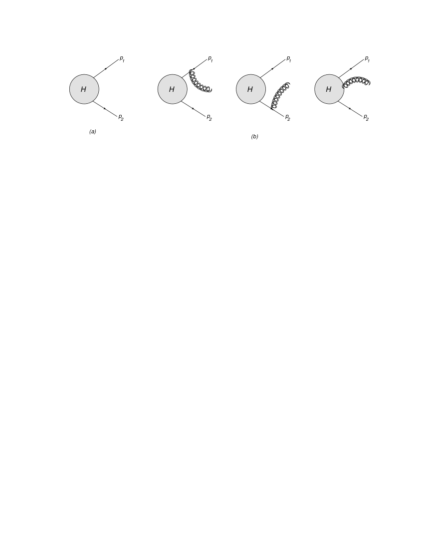
Figure 5: (a) Example vertex function involving two outgoing particles; (b) Series of diagrams involving all possible placements of an extra graviton.

For simplicity, we deal with the case of massless external particles. The vertex with no emission can then only depend on the invariant $p_{1}\cdot p_{2}$, and we denote this by $\Gamma(p_{1},p_{2})$. The full Feynman rule for emission of a graviton from a scalar is given by [1]

$$\frac{\kappa}{2}\left(p_{1\mu}\,p_{2\nu}+p_{1\nu}\,p_{2\mu}-\frac{2}{d-2}m^{2}\eta_{\mu\nu}\right)$$ (107)

in the weak field approximation of eq. (8). For $m=0$ the vertex function including an extra graviton emission (from figure 5(b)) is then

$$\Gamma_{\mu\nu} =\frac{\kappa}{2}\left[\frac{p_{1\mu}(p_{1}-k)_{\nu}+(p_{1}-k)_{\mu}p_{1\nu}}{-2p_{1}\cdot k}\Gamma[(p_{1}-k)\cdot p_{2}]\right.$$

$$\left.\quad+\frac{p_{2\mu}(p_{2}-k)_{\nu}+(p_{2}-k)_{\mu}p_{2\nu}}{-2p_{2}\cdot k}\Gamma[p_{1}\cdot(p_{2}-k)]\right]+\Gamma^{\rm int.}_{\mu\nu},$$ (108)

where $\Gamma^{\rm int.}_{\mu\nu}$ represents the contribution from the internal emission graph. It will be convenient to symmetrize on both sides, defining $\bar{\Gamma}_{\mu\nu}=\Gamma_{\mu\nu}+\Gamma_{\nu\mu}$ (and likewise for $\Gamma^{\rm int.}_{\mu\nu}$). Then eq. (108) can be rewritten

$$\frac{1}{2}\bar{\Gamma}_{\mu\nu} =\frac{\kappa}{2}\left[\frac{p_{1\mu}(p_{1}-k)_{\nu}+(p_{1}-k)_{\mu}p_{1\nu}}{-2p_{1}\cdot k}\Gamma[(p_{1}-k)\cdot p_{2}]\right.$$

$$\left.\quad+\frac{p_{2\mu}(p_{2}-k)_{\nu}+(p_{2}-k)_{\mu}p_{2\nu}}{-2p_{2}\cdot k}\Gamma[p_{1}\cdot(p_{2}-k)]\right]+\frac{1}{2}\bar{\Gamma}^{\rm int.}_{\mu\nu},$$ (109)

Expanding this to first order in $k$ gives

$$\frac{1}{2}\bar{\Gamma}_{\mu\nu} =\frac{\kappa}{2}\left[\frac{p_{1\mu}p_{1\nu}}{-p_{1}\cdot k}\left(\Gamma-p_{2}\cdot k\frac{\partial\Gamma}{\partial p_{1}\cdot p_{2}}\right)+\frac{p_{2\mu}p_{2\nu}}{-p_{2}\cdot k}\left(\Gamma-p_{1}\cdot k\frac{\partial\Gamma}{\partial p_{1}\cdot p_{2}}\right)\right.$$

$$\left.\frac{p_{1(\mu}k_{\nu)}}{2p_{1}\cdot k}\Gamma+\frac{p_{2(\mu}k_{\nu)}}{2p_{2}\cdot k}\Gamma\right]+\frac{1}{2}\bar{\Gamma}^{\rm int.}_{\mu\nu},$$ (110)

where $\Gamma\equiv\Gamma(p_{1}\cdot p_{2})$, and we have used the notation $p_{i(\mu}k_{\nu)}=p_{i\mu}k_{\nu}+p_{i\nu}k_{\mu}$. One may now use the gravitational Ward identity [74]

$$k^{\mu}\bar{\Gamma}_{\mu\nu}=0$$ (111)

(which follows from general coordinate invariance) as well as the on-shell condition for the emitted graviton ($k^{2}=0$) to find

$$\frac{1}{2}k^{\mu}\bar{\Gamma}^{\rm int.}_{\mu\nu}+\frac{\kappa}{2}\left[-p_{1\nu}\left(\Gamma-p_{2}\cdot k\frac{\partial\Gamma}{\partial p_{1}\cdot p_{2}}\right)-p_{2\nu}\left(\Gamma-p_{1}\cdot k\frac{\partial\Gamma}{\partial p_{1}\cdot p_{2}}\right)\right]=0.$$ (112)

The zeroth order term vanishes from momentum conservation ($p_{1}+p_{2}=0$). Also, one may identify

$$p_{2\mu}\frac{\partial\Gamma}{\partial p_{1}\cdot p_{2}}=\frac{\partial\Gamma}{\partial p_{1}^{\mu}},\quad p_{1\mu}\frac{\partial\Gamma}{\partial p_{1}\cdot p_{2}}=\frac{\partial\Gamma}{\partial p_{2}^{\mu}},$$ (113)

so that eq. (112) becomes

$$\bar{\Gamma}^{\rm int.}_{\mu\nu}=-\kappa\left[p_{1\nu}\frac{\partial\Gamma}{\partial p_{1}^{\mu}}+p_{2\nu}\frac{\partial\Gamma}{\partial p_{2}^{\mu}}\right].$$ (114)

This is indeed a special case of eq. (57) for internal emission graphs.

References

- [1] H. W. Hamber, Discrete and continuum quantum gravity, 0704.2895.
- [2] O. Hohm, On factorizations in perturbative quantum gravity, 1103.0032.
- [3] Z. Bern, T. Dennen, Y.-t. Huang, and M. Kiermaier, Gravity as the Square of Gauge Theory, Phys.Rev. D82 (2010) 065003, [1004.0693].
- [4] Z. Bern, J. J. M. Carrasco, and H. Johansson, Perturbative Quantum Gravity as a Double Copy of Gauge Theory, Phys.Rev.Lett. 105 (2010) 061602, [1004.0476].
- [5] Z. Bern, Perturbative quantum gravity and its relation to gauge theory, Living Rev.Rel. 5 (2002) 5, [gr-qc/0206071].
- [6] Z. Bern and A. K. Grant, Perturbative gravity from QCD amplitudes, Phys.Lett. B457 (1999) 23–32, [hep-th/9904026].
- [7] N. Arkani-Hamed and J. Kaplan, On Tree Amplitudes in Gauge Theory and Gravity, JHEP 0804 (2008) 076, [0801.2385].
- [8] Z. Bern, L. J. Dixon, D. Dunbar, M. Perelstein, and J. Rozowsky, On the relationship between Yang-Mills theory and gravity and its implication for ultraviolet divergences, Nucl.Phys. B530 (1998) 401–456, [hep-th/9802162].
- [9] Z. Bern, L. J. Dixon, and R. Roiban, Is N = 8 supergravity ultraviolet finite?, Phys.Lett. B644 (2007) 265–271, [hep-th/0611086].
- [10] Z. Bern, J. Carrasco, L. J. Dixon, H. Johansson, D. Kosower, et al., Three-Loop Superfiniteness of N=8 Supergravity, Phys.Rev.Lett. 98 (2007) 161303, [hep-th/0702112].
- [11] Z. Bern, J. Carrasco, L. J. Dixon, H. Johansson, and R. Roiban, Manifest Ultraviolet Behavior for the Three-Loop Four-Point Amplitude of N=8 Supergravity, Phys.Rev. D78 (2008) 105019, [0808.4112].
- [12] Z. Bern, J. Carrasco, L. J. Dixon, H. Johansson, and R. Roiban, The Ultraviolet Behavior of N=8 Supergravity at Four Loops, Phys.Rev.Lett. 103 (2009) 081301, [0905.2326].
- [13] S. G. Naculich and H. J. Schnitzer, Absence of subleading infrared divergences in gravity, 1101.1524. * Temporary entry *.
- [14] F. Bloch and A. Nordsieck, Note on the Radiation Field of the electron, Phys.Rev. 52 (1937) 54–59.
- [15] D. Yennie, S. C. Frautschi, and H. Suura, The infrared divergence phenomena and high-energy processes, Annals Phys. 13 (1961) 379–452.
- [16] G. F. Sterman, Summation of Large Corrections to Short Distance Hadronic Cross-Sections, Nucl.Phys. B281 (1987) 310.
- [17] S. Catani and L. Trentadue, Resummation of the QCD Perturbative Series for Hard Processes, Nucl.Phys. B327 (1989) 323.
- [18] G. Korchemsky and G. Marchesini, Structure function for large x and renormalization of Wilson loop, Nucl.Phys. B406 (1993) 225–258, [hep-ph/9210281].
- [19] G. Korchemsky and G. Marchesini, Resummation of large infrared corrections using Wilson loops, Phys.Lett. B313 (1993) 433–440.
- [20] M. Beneke, A. Chapovsky, M. Diehl, and T. Feldmann, Soft collinear effective theory and heavy to light currents beyond leading power, Nucl.Phys. B643 (2002) 431–476, [hep-ph/0206152].
- [21] C. W. Bauer, S. Fleming, D. Pirjol, and I. W. Stewart, An Effective field theory for collinear and soft gluons: Heavy to light decays, Phys.Rev. D63 (2001) 114020, [hep-ph/0011336].
- [22] C. W. Bauer, S. Fleming, D. Pirjol, I. Z. Rothstein, and I. W. Stewart, Hard scattering factorization from effective field theory, Phys.Rev. D66 (2002) 014017, [hep-ph/0202088].
- [23] T. Becher and M. Neubert, Threshold resummation in momentum space from effective field theory, Phys.Rev.Lett. 97 (2006) 082001, [hep-ph/0605050].
- [24] T. Becher, M. Neubert, and B. D. Pecjak, Factorization and Momentum-Space Resummation in Deep-Inelastic Scattering, JHEP 0701 (2007) 076, [hep-ph/0607228].
- [25] T. Becher, M. Neubert, and G. Xu, Dynamical Threshold Enhancement and Resummation in Drell-Yan Production, JHEP 0807 (2008) 030, [0710.0680].
- [26] E. Laenen, G. Stavenga, and C. D. White, Path integral approach to eikonal and next-to-eikonal exponentiation, JHEP 0903 (2009) 054, [0811.2067].
- [27] A. H. Mueller, On the asymptotic behavior of the Sudakov form-factor, Phys.Rev. D20 (1979) 2037.
- [28] J. C. Collins, Algorithm to compute corrections to the Sudakov form-factor, Phys.Rev. D22 (1980) 1478.
- [29] A. Sen, Asymptotic Behavior of the Sudakov Form-Factor in QCD, Phys.Rev. D24 (1981) 3281.
- [30] G. Korchemsky, Double logarithmic asymptotics in QCD, Phys.Lett. B217 (1989) 330–334.
- [31] L. Magnea and G. F. Sterman, Analytic continuation of the Sudakov form-factor in QCD, Phys.Rev. D42 (1990) 4222–4227.
- [32] S. Weinberg, Infrared photons and gravitons, Phys.Rev. 140 (1965) B516–B524.
- [33] L. J. Dixon, L. Magnea, and G. F. Sterman, Universal structure of subleading infrared poles in gauge theory amplitudes, JHEP 0808 (2008) 022, [0805.3515].
- [34] E. Gardi and L. Magnea, Factorization constraints for soft anomalous dimensions in QCD scattering amplitudes, JHEP 0903 (2009) 079, [0901.1091].
- [35] L. J. Dixon, Matter Dependence of the Three-Loop Soft Anomalous Dimension Matrix, Phys.Rev. D79 (2009) 091501, [0901.3414].
- [36] T. Becher and M. Neubert, Infrared singularities of scattering amplitudes in perturbative QCD, Phys.Rev.Lett. 102 (2009) 162001, [0901.0722].
- [37] T. Becher and M. Neubert, On the Structure of Infrared Singularities of Gauge-Theory Amplitudes, JHEP 0906 (2009) 081, [0903.1126].
- [38] T. Becher and M. Neubert, Infrared singularities of QCD amplitudes with massive partons, Phys.Rev. D79 (2009) 125004, [0904.1021].
- [39] L. J. Dixon, E. Gardi, and L. Magnea, On soft singularities at three loops and beyond, JHEP 1002 (2010) 081, [0910.3653].
- [40] L. J. Dixon, E. Gardi, and L. Magnea, All-order results for infrared and collinear singularities in massless gauge theories, PoS RADCOR2009 (2010) 007, [1001.4709]. * Temporary entry *.
- [41] E. Gardi and L. Magnea, Infrared singularities in QCD amplitudes, Nuovo Cim. C32N5-6 (2009) 137–157, [0908.3273].
- [42] E. Laenen, L. Magnea, G. Stavenga, and C. D. White, Next-to-eikonal corrections to soft gluon radiation: a diagrammatic approach, 1010.1860.
- [43] J. Gatheral, Exponentiation of eikonal cross-sections in nonabelian gauge theories, Phys.Lett. B133 (1983) 90.
- [44] J. Frenkel and J. C. Taylor, Nonabelian eikonal exponentiation, Nucl. Phys. B246 (1984) 231.
- [45] G. Sterman, Infrared divergences in perturbative QCD, . in Tallahassee 1981, Proceedings, Perturbative Quantum Chromodynamics, 22-40.
- [46] E. Gardi, E. Laenen, G. Stavenga, and C. D. White, Webs in multiparton scattering using the replica trick, JHEP 1011 (2010) 155, [1008.0098].
- [47] E. Gardi and C. D. White, General properties of multiparton webs: proofs from combinatorics, 1102.0756. * Temporary entry *.
- [48] A. Mitov, G. Sterman, and I. Sung, Diagrammatic Exponentiation for Products of Wilson Lines, Phys.Rev. D82 (2010) 096010, [1008.0099].
- [49] E. Laenen, L. Magnea, and G. Stavenga, On next-to-eikonal corrections to threshold resummation for the Drell-Yan and DIS cross sections, Phys.Lett. B669 (2008) 173–179, [0807.4412].
- [50] S. Moch and A. Vogt, On non-singlet physical evolution kernels and large-x coefficient functions in perturbative QCD, JHEP 11 (2009) 099, [0909.2124].
- [51] G. Soar, S. Moch, J. A. M. Vermaseren, and A. Vogt, On Higgs-exchange DIS, physical evolution kernels and fourth-order splitting functions at large x, Nucl. Phys. B832 (2010) 152, [0912.0369].
- [52] A. Vogt, G. Soar, S. Moch, and J. Vermaseren, On higher-order flavour-singlet splitting and coefficient functions at large x, 1008.0952.
- [53] A. Vogt, S. Moch, G. Soar, and J. A. M. Vermaseren, Higher-order predictions from physical evolution kernels, PoS RADCOR2009 (2010) 053, [1001.3554].
- [54] G. Grunberg and V. Ravindran, On threshold resummation beyond leading order, JHEP 10 (2009) 055, [0902.2702].
- [55] G. Grunberg, Large- structure of physical evolution kernels in Deep Inelastic Scatterin g, 0911.4471.
- [56] G. Grunberg, Threshold resummation beyond leading eikonal level, 1005.5684.
- [57] F. E. Low, Bremsstrahlung of very low-energy quanta in elementary particle collisions, Phys. Rev. 110 (1958) 974–977.
- [58] T. H. Burnett and N. M. Kroll, Extension of the low soft photon theorem, Phys. Rev. Lett. 20 (1968) 86.
- [59] V. Del Duca, High-energy bremsstrahlung theorems for soft photons, Nucl. Phys. B345 (1990) 369–388.
- [60] S. B. Giddings, M. Schmidt-Sommerfeld, and J. R. Andersen, High energy scattering in gravity and supergravity, Phys.Rev. D82 (2010) 104022, [1005.5408].
- [61] W. Stirling, E. Vryonidou, and J. Wells, Eikonal regime of gravity-induced scattering at higher energy proton colliders, 1102.3844. * Temporary entry *.
- [62] D. Capper, On quantum corrections to the graviton propagator, Nuovo Cim. A25 (1975) 29.
- [63] D. Capper, G. Leibbrandt, and M. Ramon Medrano, Calculation of the graviton selfenergy using dimensional regularization, Phys.Rev. D8 (1973) 4320–4331.
- [64] M. J. Strassler, Field theory without Feynman diagrams: One loop effective actions, Nucl.Phys. B385 (1992) 145–184, [hep-ph/9205205].
- [65] M. G. Schmidt and C. Schubert, Worldline Green functions for multiloop diagrams, Phys.Lett. B331 (1994) 69–76, [hep-th/9403158].
- [66] J. van Holten, Propagators and path integrals, Nucl.Phys. B457 (1995) 375–407, [hep-th/9508136].
- [67] Z. Bern and D. C. Dunbar, A Mapping between Feynman and string motivated one loop rules in gauge theories, Nucl.Phys. B379 (1992) 562–601.
- [68] Z. Bern and D. A. Kosower, The Computation of loop amplitudes in gauge theories, Nucl.Phys. B379 (1992) 451–561.
- [69] A. Karanikas, C. Ktorides, and N. Stefanis, World line techniques for resumming gluon radiative corrections at the cross-section level, Eur.Phys.J. C26 (2003) 445–455, [hep-ph/0210042].
- [70] G. F. Sterman, Partons, factorization and resummation, TASI 95, hep-ph/9606312.
- [71] A. Morgan, Second order fermions in gauge theories, Phys.Lett. B351 (1995) 249–256, [hep-ph/9502230].
- [72] D. Binosi, J. Collins, C. Kaufhold, and L. Theussl, JaxoDraw: A graphical user interface for drawing Feynman diagrams. Version 2.0 release notes, Comput. Phys. Commun. 180 (2009) 1709–1715, [0811.4113].
- [73] D. Binosi and L. Theussl, JaxoDraw: A graphical user interface for drawing Feynman diagrams, Comput. Phys. Commun. 161 (2004) 76–86, [hep-ph/0309015].
- [74] F. Englert and R. Brout, Gravitational Ward Identity and the Principle of Equivalence, Phys. Rev. 141 (1965) 1231.