A finite element method for nonlinear elliptic problems

Abstract.

We present a continuous finite element method for some examples of fully nonlinear elliptic equation. A key tool is the discretisation proposed in Lakkis & Pryer (2011) allowing us to work directly on the strong form of a linear PDE. An added benefit to making use of this discretisation method is that a recovered (finite element) Hessian is a biproduct of the solution process. We build on the linear basis and ultimately construct two different methodologies for the solution of second order fully nonlinear PDEs. Benchmark numerical results illustrate the convergence properties of the scheme for some test problems as well as the Monge–Ampère equation and the Pucci equation.

1. Introduction

Fully nonlinear PDEs arise in many areas, including differential geometry (the Monge–Ampère equation), mass transportation (the Monge–Kantorovich problem), dynamic programming (the Bellman equation) and fluid dynamics (the geostrophic equations). The computer approximation of the solutions of such equations is thus an important scientific task. There are at least three main difficulties apparent to someone attempting to derive numerical methods for fully nonlinear equations: first, the strong nonlinearity on the highest order derivative which generally precludes a variational formulation, second, a fully nonlinear equation does not always admit a classical solution, even if the problem data is smooth, and the solution has to sought in a generalised sense (e.g., viscosity solutions), which is bound to slow down convergence rates, and third, a common problem in nonlinear solvers, the exact solution may not be unique and constraints, such as convexity requirements must be included in the constraints to ensure uniqueness.

Regardless of the problems, the numerical approximation of fully nonlinear second order elliptic equations, as described in Caffarelli and Cabré (1995), have been the object of considerable recent research, particularly for the case of Monge–Ampère of which Oliker and Prussner (1988); Loeper and Rapetti (2005a); Dean and Glowinski (2006); Feng and Neilan (2009b); Oberman (2008); Awanou (2010); Davydov and Saeed (2012); Brenner et al. (2011a); Froese (2011) are selected examples.

For more general classes of fully nonlinear equations some methods have been presented, most notably, at least from a theoretical view point, in Böhmer (2008) where the author presents a $\operatorname{C}^{1}$ finite element method shows stability and consistency (hence convergence) of the scheme, following a classical “finite difference” approach outlined by Stetter (1973) which requires a high degree of smoothness on the exact solution. From a practical point of view this approach presents difficulties, in that the $\operatorname{C}^{1}$ finite elements are hard to design and complicated to implement, in Davydov and Saeed (2010) a useful overview of Bézier-Bernestein splines in two spatial dimensions is provided and a full implementation in Davydov and Saeed (2012). Similar difficulties are encountered in finite difference methods and the concept of wide-stencil appears to be useful, for example by Kuo and Trudinger (1992, 2005); Oberman (2008); Froese (2011).

In Feng and Neilan (2009a, b); Awanou (2010) the authors give a method in which they approximate the general second order fully nonlinear PDE by a sequence of fourth order quasilinear PDEs. These are quasilinear biharmonic equations which are discretised via mixed finite elements, or using high-regularity elements such as splines. In fact for the Monge–Ampère equation, which admits two solutions, of which one is convex and another concave, this method allows for the approximation of both solutions via the correct choice of a parameter. On the other hand although computationally less expensive than $\operatorname{C}^{1}$ finite elements (an alternative to mixed methods for solving the biharmonic problem), the mixed formulation still results in an extremely large algebraic system and the lack of maximum principle for general fourth order equations makes it hard to apply vanishing viscosity arguments to prove convergence. A somewhat different approach, based on $C^{0}$-penalty, has been recently proposed by Brenner et al. (2011a), as well as “pseudo time” one by Awanou (2011).

It is worth citing also a least square approach described by Dean and Glowinski (2006). This method consists in minimising the mean-square of the residual, using a Lagrange multiplier method. Also here a fourth order elliptic term appears in the energy.

In this paper, we depart from the above proposed methods and explore a more “direct” approach by applying the nonvariational finite element method, introduced in Lakkis and Pryer (2011), as a solver for the Newton iteration directly derived from the PDE. To be more specific, consider the following model problem

$$\mathscr{N}[u]:=F(\,\mathrm{D}^{2}u)-f=0$$ (1.1)

with homogeneous Dirichlet boundary conditions where $f:\varOmega\to\mathbb{R}$ is prescribed function and $F:\operatorname{Sym}{(\mathbb{R}^{d\times d})}\to\mathbb{R}$ is a real-valued algebraic function of symmetric matrixes, which provides an elliptic operator in the sense of Caffarelli and Cabré (1995), as explained below in Definition 2.2. The method we propose, consists in applying a Newton’s method, given below by equation (4.2) of the PDE (1.1), which results in a sequence of linear nonvariational elliptic PDEs that fall the framework of the nonvariational finite element method (NVFEM) proposed in Lakkis and Pryer (2011). The results in this paper are computational, so despite not having a complete proof of convergence, we test our algorithm various problems that are specifically constructed to be well posed. In particular, we test our method on the Monge–Ampère problem, which is the de-facto benchmark for numerical methods of fully nonlinear elliptic equations. This is in spite of Monge–Ampère having an extra complication, which is conditional ellipiticity (the operator is elliptic only if the function is convex or concave. A crucial, empirically observed feature of our method is that the convexity (or concavity) is automatically preserved if one uses $\mathbb{P}^{2}$ elements or higher. For $\mathbb{P}^{1}$ elements this is not true and the scheme must be stabilized by reenforcing convexity (or concavity) at each timestep. This was achieved in Pryer (2010) using a semidefinite programming method. In a different spirit, but somewhat reminiscent, a stabilization procedure was obtained in Brenner et al. (2011a) by adding a penalty term.

The rest of this paper is set out as follows. In §2 we introduce some notation, the model problem, discuss its ellipticity and Newton’s method, which yields a sequences of nonvariational linearised PDE’s. In §3 we review of the nonvariational finite element method proposed in Lakkis and Pryer (2011) and apply it to discretise the nonvariational linearised PDE’s in Newton’s method. In §4 we numerically demonstrate the performance of our discretisation on a class of fully nonlinear PDE, those that are elliptic and well posed without constraining our solution to a certain class of functions. In §5 we turn to conditionally elliptic problems by dealing with the prime example of such problems, i.e., Monge–Ampère . We apply the discretisation to the Monge–Ampère equation making use of the work Aguilera and Morin (2009) to check finite element convexity is preserved at each iteration. Finally in §6 we address the approximation of Pucci’s equation, which is another important example of fully nonlinear elliptic equation.

All the numerical experiments for this research, were carried out using the DOLFIN interface for FEniCS Logg and Wells (2010) and making use of Gnuplot and ParaView for the graphics.

2. Notation

2.1. Functional set-up

Let $\varOmega\subset\mathbb{R}^{d}$ be an open and bounded Lipschitz domain. We denote $\operatorname{L}_{2}(\varOmega)$ to be the space of square (Lebesgue) integrable functions on $\varOmega$ together with its inner product $\left\langle{v,w}\right\rangle:=\int_{\varOmega}vw$ and norm $\left\|v\right\|:=\left\|v\right\|_{\operatorname{L}_{2}(\varOmega)}=\left\langle{v,v}\right\rangle^{1/2}$. We denote by $\langle v\,|\,w\rangle$ the action of a distribution $v$ on the function $w$.

We use the convention that the derivative $\,\mathrm{D}u$ of a function $u:\varOmega\to\mathbb{R}$ is a row vector, while the gradient of $u$, $\nabla u$ is the derivatives transpose (an element of $\mathbb{R}^{d}$, representing $\,\mathrm{D}u$ in the canonical basis). Hence

$$\nabla u={\left(\,\mathrm{D}u\right)}^{{\boldsymbol{\intercal}}}.$$ (2.1)

For second derivatives, we follow the common innocuous abuse of notation whereby the Hessian of $u$ is denoted as $\,\mathrm{D}^{2}u$ (instead of the more consistent $\,\mathrm{D}\nabla u$) and is represented by a $d\times d$ matrix.

The standard Sobolev spaces are  Ciarlet (1978); Evans (1998)

$$\operatorname{H}^{k}(\varOmega):={\smash{\operatorname{W}}}^{k}_{2}(\varOmega)=\left\{\phi\in\operatorname{L}_{2}(\varOmega):\;\sum_{\left|\boldsymbol{\alpha}\right|\leq k}\,\mathrm{D}^{\boldsymbol{\alpha}}\phi\in\operatorname{L}_{2}(\varOmega)\right\},$$ (2.2)

$$\operatorname{H}^{1}_{0}(\varOmega):=\text{closure of }\operatorname{C}^{\infty}_{0}(\varOmega)\text{ in }\operatorname{H}^{1}(\varOmega)$$ (2.3)

where $\boldsymbol{\alpha}=\{\alpha_{1},...,\alpha_{d}\}$ is a multi-index, $\left|\boldsymbol{\alpha}\right|=\sum_{i=1}^{d}\alpha_{i}$ and derivatives $\,\mathrm{D}^{\boldsymbol{\alpha}}$ are understood in a weak sense.

We consider the case when the model problem (1.1) is uniformly elliptic in the following sense.

2.2. Definition (ellipticity Caffarelli and Cabré (1995))

The operator $\mathscr{N}[\cdot]$ in Problem (1.1) is called elliptic on $\mathscr{C}\subseteq\operatorname{Sym}{(\mathbb{R}^{d\times d})}$ if and only if for each $\boldsymbol{M}\in\mathscr{C}$ there exist $\Lambda\geq\lambda>0$, that may depend on $\boldsymbol{M}$ such that

$$\lambda\sup_{\left|\boldsymbol{\xi}\right|=1}\left|\boldsymbol{N}\boldsymbol{\xi}\right|\leq F(\boldsymbol{M}+\boldsymbol{N})-F(\boldsymbol{M})\leq\varLambda\sup_{\left|\boldsymbol{\xi}\right|=1}\left|\boldsymbol{N}\boldsymbol{\xi}\right|\quad\>\forall\>\boldsymbol{N}\in\operatorname{Sym}{(\mathbb{R}^{d\times d})}.$$ (2.4)

If the largest possible set $\mathscr{C}$ for which (2.4) is satisfied is a proper subset of $\operatorname{Sym}{(\mathbb{R}^{d\times d})}$ we say that $\mathscr{N}[\cdot]$ is conditionally elliptic.

The operator $\mathscr{N}[\cdot]$ in Problem (1.1) is called to be uniformly elliptic if and only if for some $\lambda,\varLambda>0$, called ellipticity constants, we have

$$\lambda\sup_{\left|\boldsymbol{\xi}\right|=1}\left|\boldsymbol{N}\boldsymbol{\xi}\right|\leq F(\boldsymbol{M}+\boldsymbol{N})-F(\boldsymbol{M})\leq\varLambda\sup_{\left|\boldsymbol{\xi}\right|=1}\left|\boldsymbol{N}\boldsymbol{\xi}\right|\quad\>\forall\>\boldsymbol{N},\boldsymbol{M}\in\operatorname{Sym}{(\mathbb{R}^{d\times d})}.$$ (2.5)

If $F$ is differentiable (2.5) can be obtained from conditions on the derivative of $F$. A generic $\boldsymbol{M}\in\operatorname{Sym}{(\mathbb{R}^{d\times d})}$ is written as

$$\boldsymbol{M}=\begin{bmatrix}{m}_{1,1}&\dotsc&{m}_{1,d}\\ \vdots&\ddots&\vdots\\ {m}_{d,1}&\dotsc&{m}_{d,d}\end{bmatrix};$$ (2.6)

so the derivative of $F$ in the direction $\boldsymbol{N}$ is given by

$$\,\mathrm{D}F(\boldsymbol{M})\boldsymbol{N}={F^{\prime}(\boldsymbol{M})}{:}{\boldsymbol{N}}$$ (2.7)

where the derivative matrix $F^{\prime}(\boldsymbol{M})$ is defined by

$$F^{\prime}(\boldsymbol{M}):=\begin{bmatrix}{\partial F(\boldsymbol{M})/\partial m}_{1,1}&\dotsc&{\partial F(\boldsymbol{M})/\partial m}_{1,d}\\ \vdots&\ddots&\vdots\\ {\partial F(\boldsymbol{M})/\partial m}_{d,1}&\dotsc&{\partial F(\boldsymbol{M})/\partial m}_{d,d}\end{bmatrix}.$$ (2.8)

Suppose $F$ is differentiable. Then (2.4) is satisfied if and only if for each $\boldsymbol{M}\in\mathscr{C}$ there exists $\mu>0$ such that

$${\boldsymbol{\xi}}^{{\boldsymbol{\intercal}}}F^{\prime}(\boldsymbol{M})\boldsymbol{\xi}\geq\mu\left|\boldsymbol{\xi}\right|^{2}\quad\>\forall\>\boldsymbol{\xi}\in\mathbb{R}^{d}.$$ (2.9)

Furthermore $\mathscr{C}=\operatorname{Sym}{(\mathbb{R}^{d\times d})}$ and $\mu$ is independent of $\boldsymbol{M}$ if and only if (2.5) is satisfied.

2.3. Assumption (smooth elliptic operator)

In the remainder of this paper we shall assume that $\mathscr{N}[\cdot]$ is conditionally elliptic on $\mathscr{C}$ and

$$F\in\operatorname{C}^{1}(\mathscr{C}).$$ (2.10)

Unless otherwise stated we will also assume that $\mathscr{C}=\operatorname{Sym}{(\mathbb{R}^{d\times d})}$.

2.4. Newton’s method

The smoothness assumption 2.3 allows to apply Newton’s method to solve Problem (1.1).

Given the initial guess $u^{0}\in\operatorname{C}^{2}(\varOmega)$, with $\,\mathrm{D}^{2}u^{0}\in\mathscr{C}$, for each $n\in\mathbb{N}_{0}$, find $u^{n+1}\in\operatorname{C}^{2}(\varOmega)$ with $\,\mathrm{D}^{2}u^{n+1}\in\mathscr{C}$ such that

$$\,\mathrm{D}\mathscr{N}[u^{n}]\left(u^{n+1}-u^{n}\right)=-\mathscr{N}[u^{n}],$$ (2.11)

where $\,\mathrm{D}\mathscr{N}[u]$ indicates the (Fréchet) derivative, which is formally given by

$$\begin{split}{\,\mathrm{D}\mathscr{N}[u]}{v}&=\lim_{\epsilon\rightarrow 0}\frac{\mathscr{N}[u+\epsilon v]-\mathscr{N}[u]}{\epsilon}\\ &=\lim_{\epsilon\rightarrow 0}\frac{F(\,\mathrm{D}^{2}u+\epsilon\,\mathrm{D}^{2}v)-F(\,\mathrm{D}^{2}u)}{\epsilon}\\ &=F^{\prime}(\,\mathrm{D}^{2}u):\,\mathrm{D}^{2}v,\end{split}$$ (2.12)

for each $v\in\operatorname{C}^{2}(\varOmega)$. Combining (2.11) and (2.12) then results in the following nonvariational sequence of linear PDEs. Given $u^{0}$ for each $n\in\mathbb{N}_{0}$ find $u^{n+1}$ such that

$$F^{\prime}(\,\mathrm{D}^{2}u^{n}):\,\mathrm{D}^{2}\left(u^{n+1}-u^{n}\right)=f-F(\,\mathrm{D}^{2}u^{n}).$$ (2.13)

The PDE (2.13) comes naturally in a nonvariational form. If we attempted to rewrite into a variational form, in order, say, to apply a “standard” Galerkin method, we would introduce an advection term which would depend on derivatives of $F^{\prime}$, i.e., for generic $v,w$

$${F^{\prime}(\,\mathrm{D}^{2}v)}{:}{\,\mathrm{D}^{2}w}=\operatorname{div}\!\left[{F^{\prime}(\,\mathrm{D}^{2}v)\nabla w}\right]-\operatorname{div}\!\left[{F^{\prime}(\,\mathrm{D}^{2}v)}\right]\nabla w.$$ (2.14)

where the matrix-divergence is taken row-wise:

$$\operatorname{div}\!\left[{F^{\prime}(\,\mathrm{D}^{2}v(\boldsymbol{x}))}\right]:=\!\left({\sum_{i=1}^{d}\frac{\partial}{\partial x_{i}}\!\left[{{F^{\prime}}_{i,1}(\,\mathrm{D}^{2}v(\boldsymbol{x}))}\right],\dotsc,\sum_{i=1}^{d}\frac{\partial}{\partial x_{i}}\!\left[{{F^{\prime}}_{i,d}(\,\mathrm{D}^{2}v(\boldsymbol{x}))}\right]}\right)$$ (2.15)

and the chain rule provides us, for each $j=1,\ldots,d$, with

$$\sum_{i=1}^{d}\frac{\partial}{\partial x_{i}}\!\left[{{F^{\prime}}_{i,j}(\,\mathrm{D}^{2}v(\boldsymbol{x}))}\right]=\sum_{k,l=1}^{d}\partial_{k,l}{F^{\prime}}_{i,j}(\,\mathrm{D}^{2}v(\boldsymbol{x}))\partial_{ikl}v(\boldsymbol{x}).$$ (2.16)

This procedure is undesirable for many reasons. Firstly it requires $F$ to be twice differentiable and it involves a third order derivative of the functions $u^{n+1}$ and $u^{n}$ appearing in (2.11). Moreover, the “variational” reformulation could very well result in the problem becoming advection dominated and unstable for conforming FEM, as was manifested in numerical examples for the linear equation (Lakkis and Pryer, 2011, §4.2). In order to avoid these problems, we here propose the use of the nonvariational finite element method described next.

3. The nonvariational finite element method

In Lakkis and Pryer (2011) we proposed the nonvariational finite element method (NVFEM) to approximate the solution of problems of the form (2.13). We review here the NVFEM and explain how to use it in combination with the Newton method to derive a practical Galerkin method for the numerical approximation of Problem (1.1)’s solution.

3.1. Distributional form of (2.13) and generalised Hessian

Let $\boldsymbol{A}\in\operatorname{L}_{\infty}(\varOmega)^{d\times d}$ and for each $\boldsymbol{x}\in\varOmega$, let $\boldsymbol{A}(\boldsymbol{x})\in\operatorname{Sym}{(\mathbb{R}^{d\times d})}$, the space of bounded, symmetric, positive definite, $d\times d$ matrices and $f:\varOmega\to\mathbb{R}$. The Dirichlet linear nonvariational elliptic problem associated with $\boldsymbol{A}$ and $f$ is

$${\boldsymbol{A}}{:}{\,\mathrm{D}^{2}}u=f\text{ and }\left.u\right|_{\partial\varOmega}=0.$$ (3.1)

Testing this equation, and assuming $u\in\operatorname{H}^{2}(\varOmega)\cap\operatorname{H}^{1}_{0}(\varOmega)$ such that $\left.\nabla u\right|_{\partial\varOmega}\in\operatorname{L}_{2}(\partial\varOmega)$, we may write it as

$$\begin{split}\left\langle{{\boldsymbol{A}}{:}{\,\mathrm{D}^{2}u},\phi}\right\rangle&=\left\langle{f,\phi}\right\rangle\qquad\quad\>\forall\>\phi\in\operatorname{C}^{\infty}_{0}(\varOmega).\end{split}$$ (3.2)

To allow a Galerkin type discretisation of (3.2), we need to restrict the test functions $\phi$ to finite element function spaces that are generally not subspaces of $\operatorname{H}^{2}(\varOmega)$. So before restricting, we need to extend and we use a traditional distribution-theory (or generalised-functions) approach. Given a function $v\in\operatorname{H}^{2}(\varOmega)$ and let $\boldsymbol{n}:\partial\varOmega\to\mathbb{R}^{d}$ be the outward pointing normal of $\varOmega$ then the Hessian of $v$, $\,\mathrm{D}^{2}v$ satisfies the following identity:

$$\left\langle{\,\mathrm{D}^{2}v,\phi}\right\rangle=-\int_{\varOmega}\nabla v\otimes\nabla\phi+\int_{\partial\varOmega}\nabla v\otimes\boldsymbol{n}\,\phi\quad\>\forall\>\phi\in\operatorname{H}^{1}(\varOmega),$$ (3.3)

where $\boldsymbol{a}\otimes\boldsymbol{b}:=\boldsymbol{a}{\boldsymbol{b}}^{{\boldsymbol{\intercal}}}$ for $\boldsymbol{a},\boldsymbol{b}$ column vectors in $\mathbb{R}^{d}$. If $v\in\operatorname{H}^{1}(\varOmega)$ with $\left.\nabla v\right|_{\partial\varOmega}\in\operatorname{H}^{-1/2}(\partial\varOmega)$ the right-hand side of (3.3) still makes sense and defines $\,\mathrm{D}^{2}v$ as an element in the dual of $\operatorname{H}^{1}(\varOmega)$ via

$$\langle\,\mathrm{D}^{2}v\,|\,\phi\rangle:=-\int_{\varOmega}\nabla v\otimes\nabla\phi+\int_{\partial\varOmega}\nabla v\otimes\boldsymbol{n}\,\phi\quad\>\forall\>\phi\in\operatorname{H}^{1}(\varOmega),$$ (3.4)

where $\langle\cdot\,|\,\cdot\rangle$ denotes the duality action on $\operatorname{H}^{1}(\varOmega)$ from its dual. We call $\,\mathrm{D}^{2}v$ the generalised Hessian of $v$, and assuming that the coefficient tensor $\boldsymbol{A}$ is in $\operatorname{C}^{0}(\varOmega)^{d\times d}$, for the product with a distribution to make sense, we now seek $u\in\operatorname{H}^{1}_{0}(\varOmega)$ such that $\left.\nabla u\right|_{\partial\varOmega}\in\operatorname{H}^{-1/2}(\varOmega)$ and whose generalised Hessian satisfies

$$\langle{\boldsymbol{A}}{:}{\,\mathrm{D}^{2}}v\,|\,\phi\rangle=\left\langle{f,\phi}\right\rangle\quad\>\forall\>\phi\in\operatorname{H}^{1}(\varOmega).$$ (3.5)

3.2. Finite element discretisation and finite element Hessian

We discretise (3.5) for simplicity with a standard piecewise polynomial approximation for test and trial spaces for both problem variable, $U$, and auxiliary (mixed-type) variable, $\boldsymbol{H}[U]$. Let $\mathscr{T}$ be a conforming, shape regular triangulation of $\varOmega$, namely, $\mathscr{T}$ is a finite family of sets such that

1. $K\in\mathscr{T}$ implies $K$ is an open simplex (segment for $d=1$, triangle for $d=2$, tetrahedron for $d=3$),

2. for any $K,J\in\mathscr{T}$ we have that $\overline{K}\cap\overline{J}$ is a full subsimplex (i.e., it is either $\emptyset$, a vertex, an edge, a face, or the whole of $\overline{K}$ and $\overline{J}$) of both $\overline{K}$ and $\overline{J}$ and

3. $\bigcup_{K\in\mathscr{T}}\overline{K}=\overline{\varOmega}$.

We use the convention where $h:\varOmega\to\mathbb{R}$ denotes the meshsize function of $\mathscr{T}$, i.e.,

$$h(\boldsymbol{x}):=\max_{\overline{K}\ni\boldsymbol{x}}h_{K}.$$ (3.6)

We introduce the finite element spaces

$$\mathbb{V}:=\left\{\Phi\in\operatorname{H}^{1}(\varOmega):\;\Phi|_{K}\in\mathbb{P}^{p}\>\forall\>K\in\mathscr{T}\text{ and }\Phi\in\operatorname{C}^{0}(\varOmega)\right\},$$ (3.7)

$$\mathring{\mathbb{V}}:=\mathbb{V}\cap\operatorname{H}^{1}_{0}(\varOmega),$$ (3.8)

where $\mathbb{P}^{k}$ denotes the linear space of polynomials in $d$ variables of degree no higher than a positive integer $k$. We consider $p\geq 1$ to be fixed and denote by $\mathring{N}:=\dim{\mathring{\mathbb{V}}}$ and $N:=\dim{\mathbb{V}}$. The discretisation of problem then reads: Find $(U,\boldsymbol{H}[U])\in\mathring{\mathbb{V}}\times\mathbb{V}^{d\times d}$ such that

$$\begin{gathered}\left\langle{\boldsymbol{H}[U],\Phi}\right\rangle=-\int_{\varOmega}{\nabla U}\otimes{\nabla\Phi}+\int_{\partial\varOmega}{\nabla U}\otimes{\boldsymbol{n}\ \Phi}\quad\>\forall\>\Phi\in\mathbb{V},\\ \left\langle{{\boldsymbol{A}}{:}{\boldsymbol{H}[U]},\Psi}\right\rangle=\left\langle{f,\Psi}\right\rangle\quad\>\forall\>\Psi\in\mathring{\mathbb{V}}.\end{gathered}$$ (3.9)

For an algebraic formulation of (3.9) we refer the reader to (Lakkis and Pryer, 2011, §2). Note that this discretisation can be interpreted as a mixed method whereby the first (matrix) equation defines the finite element Hessian and the second (scalar) equation approximates the original PDE (3.2).

3.3. Two discretisation stategies of (1.1)

The finite element Hessian allows us two discretisation strategies. The first strategy, detailed in §4, consists in applying Newton first to set-up (2.13) and then using the NVFEM (3.9) to solve each step. A second strategy becomes possible, upon noting that given $U\in\mathbb{V}$ the finite element Hessian $\boldsymbol{H}[U]$ is a regular function, which the generalised Hessian $\,\mathrm{D}^{2}U$ might fail to be. This allows to apply nonlinear functions such as $F$ to $\boldsymbol{H}[U]$ and consider the following fully nonlinear finite element method (FNFEM)

$$\begin{gathered}\left\langle{\boldsymbol{H}[U],\Phi}\right\rangle=-\int_{\varOmega}{\nabla U}\otimes{\nabla\Phi}+\int_{\partial\varOmega}{\nabla U}\otimes{\boldsymbol{n}\ \Phi}\quad\>\forall\>\Phi\in\mathbb{V},\\ \left\langle{F(\boldsymbol{H}[U]),\Psi}\right\rangle=\left\langle{f,\Psi}\right\rangle\quad\>\forall\>\Psi\in\smash{\mathring{\mathbb{V}}}^{.}\end{gathered}$$ (3.10)

Of course, in order to solve the second equation, a finite-dimensional Newton method may be necessary (but this strategy leaves the door open for other nonlinear solvers, e.g., fixed point iterations). A finite element code based on this idea will be tested in §6 to solve the Pucci equation.

In summary the finite element Hessian allows both paths in the following diagram:

(3.11)

Although the diagram in (3.11) does not generally commute, if the function $F$ is algebraically accessible, then it is commutative. By “algebraically accessible” we mean a function that can be computed in a finite number of algebraic operations or inverses thereof. In this paper, we use only algebraically accessible nonlinearities, but, in principle assuming derivatives are available, our methods could be extended to algebraically inaccessible nonlinearities, such as Bellman’s (or Isaacs’s) operators involving optimums over infinite families, e.g.,

$$F(\boldsymbol{M}):=\inf_{\alpha\in\mathscr{A}}{\boldsymbol{L}_{\alpha}}{:}{\boldsymbol{M}}\quad\big{(}\!\text{ or }F(\boldsymbol{M}):=\inf_{\alpha\in\mathscr{A}}\sup_{\beta\in\mathscr{B}}{\boldsymbol{L}_{\alpha,\beta}}{:}{\boldsymbol{M}}\!\big{)},$$ (3.12)

where $\left\{\boldsymbol{L}_{\alpha}:\;\alpha\in\mathscr{A}\right\}$ (or $\left\{\boldsymbol{L}_{\alpha,\beta}:\;(\alpha,\beta)\in\mathscr{A}\times\mathscr{B}\right\}$) is a family of elliptic operators.

4. The discretisation of unconstrained fully nonlinear PDEs

In this section we detail the application of the method reviewed in §3 to the fully nonlinear model problem (1.1). Many fully nonlinear elliptic PDEs must be constrained in order to admit a unique solution. For example the Monge–Ampère–Dirichlet is elliptic and admits a unique solution in the cone of convex (or concave) functions when $f>0$ (or $f<0$, respectively). Before we turn our attention to the more complicated constrained PDE’s in §5 and we illustrate the Newton–NVFEM method in the simplest light. In this section we study fully nonlinear PDEs which have no such constraint.

4.1. Assumption (unconditionally elliptic linearisation)

We assume, in this section, that the Newton-step linearisation (2.13) is elliptic. For this assumption to hold, it is sufficient to assume uniform ellipticity, i.e., (2.9) with $\mathscr{C}=\operatorname{Sym}{(\mathbb{R}^{d\times d})}$ and $\mu>0$ independent of $\boldsymbol{M}$.

4.2. The Newton-NVFEM method

Suppose we are given a BVP of the form, finding $u\in\operatorname{H}^{2}(\varOmega)\cap\operatorname{H}^{1}_{0}(\varOmega)$ such that

$$\begin{split}\mathscr{N}[u]=F(\,\mathrm{D}^{2}u)-f&=0\qquad\text{ in }\varOmega,\end{split}$$ (4.1)

which satisfies Assumption 4.1.

Upon applying Newton’s method to approximate the solution of problem (4.1) we obtain a sequence of functions $(u^{n})_{n\in\mathbb{N}_{0}}$ solving the following linear equations in nonvariational form,

$${\boldsymbol{N}(\,\mathrm{D}^{2}u^{n})}{:}{\,\mathrm{D}^{2}u^{n+1}}=g(\,\mathrm{D}^{2}u^{n})$$ (4.2)

where

$$\boldsymbol{N}(\boldsymbol{X}):=F^{\prime}(\boldsymbol{X}),$$ (4.3)

$$g(\boldsymbol{X}):=f-F(\boldsymbol{X})+{F^{\prime}(\boldsymbol{X})}{:}{\boldsymbol{X}}.$$ (4.4)

The nonlinear finite element method to approximate (4.2) is: given an initial guess $U^{0}:=\Pi_{0}u^{0}$ for each $n\in\mathbb{N}_{0}$ find $(U^{n+1},\boldsymbol{H}[U^{n+1}])\in\mathring{\mathbb{V}}\times\mathbb{V}^{d\times d}$ such that

$$\begin{gathered}\left\langle{\boldsymbol{H}[U^{n+1}],\Phi}\right\rangle+\int_{\varOmega}{\nabla U^{n+1}}\otimes{\nabla\Phi}-\int_{\partial\varOmega}{\nabla U^{n+1}}\otimes{\boldsymbol{n}}\,\Phi=\boldsymbol{0}\quad\>\forall\>\Phi\in\mathbb{V}\\ \text{ and }\left\langle{{\boldsymbol{N}(\boldsymbol{H}[U^{n}])}{:}{\boldsymbol{H}[U^{n+1}]},\Psi}\right\rangle=\left\langle{g(\boldsymbol{H}[U^{n}]),\Psi}\right\rangle\quad\>\forall\>\Psi\in\mathring{\mathbb{V}}.\end{gathered}$$ (4.5)

4.3. Remark (initial conditions)

4.4. Numerical experiments: a simple example

In this section we detail numerical experiments aimed at demonstrating the application of (4.5) to a simple model problem.

4.5. Example (a simple fully nonlinear PDE)

The first example we consider is a fully nonlinear PDE with a very smooth nonlinearity. The problem is

$$\begin{split}\mathscr{N}[u]:=\operatorname{sin}\left(\Delta u\right)+2\Delta u-f&=0\text{ in }\varOmega,\\ u&=0\text{ on }\partial\varOmega.\end{split}$$ (4.6)

which is specifically constructed to be uniformly elliptic. Indeed

$$F^{\prime}(\,\mathrm{D}^{2}u)=\left(\operatorname{cos}\left(\Delta u\right)+2\right)\operatorname{\bf I}.$$ (4.7)

which is uniformly positive definite. The Newton linearisation of the problem is then: Given $u^{0}$, for $n\in\mathbb{N}_{0}$ find $u^{n+1}$ such that

$${\left(\operatorname{cos}\left(\Delta u^{n}\right)+2\right)\operatorname{\bf I}}{:}{\,\mathrm{D}^{2}(u^{n+1}-u^{n})}=f-\operatorname{sin}\left(\Delta u^{n}\right)-2\Delta u^{n}.$$ (4.8)

and our approximation scheme is nothing but 4.5 with

$$\boldsymbol{N}(\boldsymbol{X})=\left(\operatorname{cos}\left(\operatorname{trace}{\boldsymbol{X}}\right)+2\right)\boldsymbol{I}$$ (4.9)

$$g(\boldsymbol{X})=f-\operatorname{sin}\left(\operatorname{trace}{\boldsymbol{X}}\right)-2\operatorname{trace}{\boldsymbol{X}}.$$ (4.10)

Figure 1 details a numerical experiment on this problem when $d=2$ and when $\varOmega=[-1,1]^{2}$ is a square which is triangulated using a criss-cross mesh.

4.6. Remark (simplification of Example 4.5)

Example 4.5 can be simplified considerably by noticing that

$$\int_{\varOmega}\operatorname{tr}{\boldsymbol{H}[U]}\Phi=\int_{\varOmega}{\!\left({\nabla U}\right)}^{{\boldsymbol{\intercal}}}\nabla\Phi\quad\>\forall\>\Phi\in\mathring{\mathbb{V}}.$$ (4.11)

This coincides with the definition of the discrete Laplacian and makes the NVFEM coincide with the standard conforming FEM. This observation applies to all fully nonlinear equations, with nonlinearity of the form (1.1) with

$$F(\boldsymbol{M}):=a(\operatorname{tr}{\boldsymbol{M}}),$$ (4.12)

for some given $a$. This class of problems, can be solved using a variational finite element method and can be used for comparison with our method. Note that in Jensen and Smears (2012) the authors use this together with a localisation argument in order to prove convergence of a finite element method for a specific class of Hamilton–Jacobi–Bellman equation. Their method coincides with ours, for an appropriate choice of quadrature.

Figure 1. Numerical experiments for Example 4.5. Choosing $f$ appropriately such that $u(\boldsymbol{x})=\exp\!\left({-10\left|\boldsymbol{x}\right|^{2}}\right)$. We use an initial guess $u^{0}=0$ and run the iterative procedure until $\left\|U^{n+1}-U^{n}\right\|\leq 10^{-8}$, setting $U:=U^{M}$ the final Newton iterate of the sequence. Here we are plotting log–log error plots together with experimental convergence rates for $\operatorname{L}_{2}(\varOmega),\operatorname{H}^{1}(\varOmega)$ error functionals for the problem variable, $U$, and an $\operatorname{L}_{2}(\varOmega)$ error functional for the auxiliary variable, $\boldsymbol{H}[U]$. Notice that there is a “superconvergence” of the auxiliary variable for both approximations.

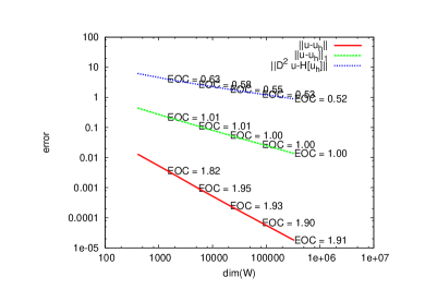
(a) Taking $\mathbb{V}$ to be the space of piecewise linear functions on $\varOmega$ ($p=1$). Notice that $\left\|u-U^{M}\right\|=\operatorname{O}(h^{2})$, $\left|u-U^{M}\right|_{1}=\operatorname{O}(h)$ and $\left\|\,\mathrm{D}^{2}u-\boldsymbol{H}[U^{M}]\right\|=\operatorname{O}(h^{0.5})$.

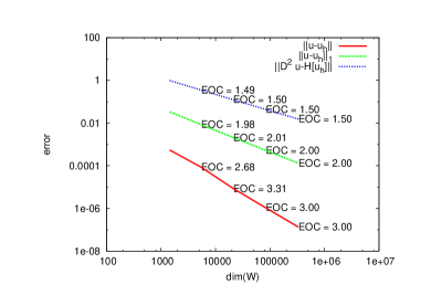
(b) Taking $\mathbb{V}$ to be the space of piecewise quadratic functions on $\varOmega$ ($p=2$). Notice that $\left\|u-U^{M}\right\|=\operatorname{O}(h^{3})$, $\left|u-U^{M}\right|_{1}=\operatorname{O}(h^{2})$ and $\left\|\,\mathrm{D}^{2}u-\boldsymbol{H}[U^{M}]\right\|=\operatorname{O}(h^{1.5})$

4.7. Example (nonvariational example)

This is a simple example where the variational trick mentioned in Remark 4.6 cannot be applied. We fix $d=2$ and consider the problem

$$\begin{split}\mathscr{N}[u]:=\!\left({\partial_{11}u}\right)^{3}+\!\left({\partial_{22}u}\right)^{3}+\partial_{11}u+\partial_{22}u-f&=0\text{ in }\varOmega\\ u&=0\text{ on }\partial\varOmega.\end{split}$$ (4.13)

The approximation scheme is then (4.5) with

$$\boldsymbol{N}(\boldsymbol{X}):=\begin{bmatrix}3\boldsymbol{X}_{11}^{2}+1&0\\ 0&3\boldsymbol{X}_{22}^{2}+1\end{bmatrix}$$ (4.14)

$$g(\boldsymbol{X}):=f+2\!\left({\boldsymbol{X}_{11}^{3}+\boldsymbol{X}_{22}^{3}}\right).$$ (4.15)

Figure 2 details a numerical experiment on this problem in the case $d=2$ and $\varOmega=[-1,1]^{2}$ triangulated with a criss-cross mesh. A similar example is also studied in (Davydov and Saeed, 2012, Ex 5.2) using Böhmers method.

Figure 2. Numerical experiments for Example 4.7. Choosing $f$ appropriately such that $u(\boldsymbol{x})=\exp\!\left({-10\left|\boldsymbol{x}\right|^{2}}\right)$. We use an initial guess $u^{0}=0$ and run the iterative procedure until $\left\|U^{n+1}-U^{n}\right\|\leq 10^{-8}$, setting $U:=U^{M}$ the final Newton iterate of the sequence. Here we are plotting log–log error plots together with experimental convergence rates for $\operatorname{L}_{2}(\varOmega),\operatorname{H}^{1}(\varOmega)$ error functionals for the problem variable, $U$, and an $\operatorname{L}_{2}(\varOmega)$ error functional for the auxiliary variable, $\boldsymbol{H}[U]$. Notice that there is a “superconvergence” of the auxiliary variable for both approximations.

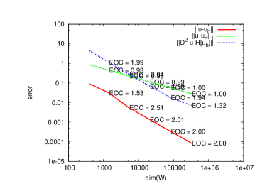
(a) Taking $\mathbb{V}$ to be the space of piecewise linear functions on $\varOmega$ ($p=1$). Notice that $\left\|u-U^{M}\right\|=\operatorname{O}(h^{2})$, $\left|u-U^{M}\right|_{1}=\operatorname{O}(h)$ and $\left\|\,\mathrm{D}^{2}u-\boldsymbol{H}[U^{M}]\right\|\approx\operatorname{O}(h^{1.5})$.

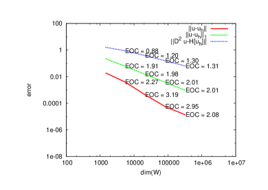
(b) Taking $\mathbb{V}$ to be the space of piecewise quadratic functions on $\varOmega$ ($p=2$). Notice that $\left\|u-U^{M}\right\|=\operatorname{O}(h^{3})$, $\left|u-U^{M}\right|_{1}=\operatorname{O}(h^{2})$ and $\left\|\,\mathrm{D}^{2}u-\boldsymbol{H}[U^{M}]\right\|=\operatorname{O}(h^{1.3})$

5. The Monge–Ampère–Dirichlet problem

In this section we propose a numerical method for the Monge–Ampère–Dirichlet (MAD) problem

$$\begin{split}\operatorname{det}\,\mathrm{D}^{2}u&=f\text{ in }\varOmega\\ u&=g\text{ on }\partial\varOmega.\end{split}$$ (5.1)

Our numerical experiments exhibit robustness of our method when computing (smooth) classical solutions of the MAD equation. Most importantly we noted the following facts:

1. the use of $\mathbb{P}^{p}$ elements with $p\geq 2$ is essential as $\mathbb{P}^{1}$ do not work,

2. the convexity of the Newton iterates is conserved throughout the computation, in a similar way to the observations in Loeper and Rapetti (2005b), where the authors prove this convexity-conservation property.

Our observations are purely empirical from computations, which leaves an interesting open problem of proving this property.

5.1. Remark (the MAD problem fails to satisfy Assumption 4.1)

To clarify Assumption 4.1 for the MAD problem (5.1), in view of the characteristic expansion of determinant if $\boldsymbol{X},\boldsymbol{Y}\in\operatorname{Sym}{(\mathbb{R}^{d\times d})}$

$$\operatorname{det}\!\left({\boldsymbol{X}+\epsilon\boldsymbol{Y}}\right)=\operatorname{det}\boldsymbol{X}+\epsilon{\operatorname{Cof}\!\left({\boldsymbol{X}}\right)}{:}{\boldsymbol{Y}}+\operatorname{O}(\epsilon^{2}),$$ (5.2)

where $\operatorname{Cof}\boldsymbol{X}$ is the matrix of cofactors of $\boldsymbol{X}$. Hence

$$F^{\prime}(\boldsymbol{X})=\operatorname{Cof}\boldsymbol{X}.$$ (5.3)

This implies that the linearisation of MAD is only well posed if we restrict the class of functions we consider to those $u$ that satisfy

$${\boldsymbol{\xi}}^{{\boldsymbol{\intercal}}}\operatorname{Cof}\,\mathrm{D}^{2}u\,\boldsymbol{\xi}\geq\lambda\left|\boldsymbol{\xi}\right|^{2}\quad\>\forall\>\boldsymbol{\xi}\in\mathbb{R}^{d}$$ (5.4)

for some ($u$-dependent) $\lambda>0$. Note that (5.4) is equivalent to the following two conditions as well

$$\begin{gathered}{\boldsymbol{\xi}}^{{\boldsymbol{\intercal}}}\,\mathrm{D}^{2}u\,\boldsymbol{\xi}\geq\lambda\left|\boldsymbol{\xi}\right|^{2}\quad\>\forall\>\boldsymbol{\xi}\in\mathbb{R}^{d}\\ $u$\text{ is strictly convex. }\end{gathered}$$ (5.5)

Loeper and Rapetti (2005a) have shown that for the continuous (infinite dimensional) Newton method described in 2.4, given an strictly convex initial guess $u^{0}$, each iterate $u^{n}$ will be convex. It is crucial that this property is preserved at the discrete level, as it guarantees the solvability of each iteration in the discretised Newton method. For this it the right notion of convexity turns out to be the finite element convexity as developed in Aguilera and Morin (2009). In Pryer (2010), an intricate method based on semidefinite programming provided a way to constrain the solution in the case of $\mathbb{P}^{1}$ elements. Here we observe that the finite element convexity is automatically preserved, provided we use $\mathbb{P}^{2}$ or higher conforming elements.

5.2. Newton’s method applied to Monge–Ampère

In view of (5.3) it is clear that

$$\,\mathrm{D}\mathscr{N}[u]v={\operatorname{Cof}\,\mathrm{D}^{2}u}{:}{\,\mathrm{D}^{2}v}.$$ (5.6)

Applying the methodology set out in §4 we set

$$\boldsymbol{N}(\,\mathrm{D}^{2}u^{n})=\operatorname{Cof}\,\mathrm{D}^{2}u^{n},$$ (5.7)

$$g(\,\mathrm{D}^{2}u^{n})=f-\operatorname{det}\,\mathrm{D}^{2}u^{n}+{\operatorname{Cof}\,\mathrm{D}^{2}u^{n}}{:}{\,\mathrm{D}^{2}u^{n}},$$ (5.8)

5.3. Remark (relating cofactors to determinants)

For a generic (twice differentiable) function $v$ it holds that

$$d\operatorname{det}\,\mathrm{D}^{2}v={\operatorname{Cof}\,\mathrm{D}^{2}v}{:}{\,\mathrm{D}^{2}v}.$$ (5.9)

Using this formulation we could construct a simple fixed point method for the Monge–Ampère equation. In view of Remark 5.3 $g$ can be further simplified

$$\begin{split}g(\,\mathrm{D}^{2}u^{n})&=f-\operatorname{det}\,\mathrm{D}^{2}u^{n}+{\operatorname{Cof}\,\mathrm{D}^{2}u^{n}}{:}{\,\mathrm{D}^{2}u^{n}}\\ &=f+(d-1)\operatorname{det}\,\mathrm{D}^{2}u^{n}.\end{split}$$ (5.10)

Newton’s method reads: Given $u^{0}$ for each $n\in\mathbb{N}_{0}$ find $u^{n+1}$ such that

$${\boldsymbol{N}(\,\mathrm{D}^{2}u^{n})}{:}{\,\mathrm{D}^{2}u^{n+1}}=g(\,\mathrm{D}^{2}u^{n}).$$ (5.11)

5.4. Numerical experiments

In this section we study the numerical behaviour of the scheme presented in Definition 4.2 applied to the MAD problem.

We present a set of benchmark problems constructed from the problem data such that the solution to the Monge–Ampère equation is known. We fix $\varOmega$ to be the square $S=[-1,1]^{2}$ or $[0,1]^{2}$ (specified in the problem) and test convergence rates of the discrete solution to the exact solution.

Figures 3–6 details the various experiments and shows numerical convergence results for each of the problems studied as well as solution plots, it is worthy of note that each of the solutions seems to be convex, however this is not necessarily the case. They are all though finite element convex Aguilera and Morin (2009). In each of these cases the Dirichlet boundary values are not zero. The implementation of nontrivial boundary conditions is described in (Lakkis and Pryer, 2011, §3.6) or in more detail in (Pryer, 2010, §4.4).

5.5. Remark (choosing the “right” initial guess)

As with any Newton method we require a starting guess, not just for $U^{0}$ but also of $\boldsymbol{H}[U^{0}]$. Due to the mild nonlinearity with the previous example an initial guess of $U^{0}\equiv 0$ and $\boldsymbol{H}[U^{0}]\equiv\boldsymbol{0}$ was sufficient. The initial guess to the MAD problem must be more carefully sought.

Since we restrict our solution to the space of convex functions, it is prudent for the initial guess to also be convex. Moreover we must rule out constant and linear functions over $\varOmega$, since the Hessian of these objects would be identically zero, destroying ellipticity on the initial Newton step. Hence we specify that the initial guess to (5.11) must be strictly convex. Rather than postprocessing the finite element Hessian from a initial project (although this is an option) to initialise the algorithm we solve a linear problem using the nonvariational finite element method. Following a trick, described in Dean and Glowinski (2003), we chose $U^{0}$ to be the standard $\mathbb{V}$-finite element approximation of $u^{0}$ such that

$$\Delta u^{0}=2\sqrt{f}\text{ in }\varOmega$$ (5.12)

$$u^{0}=g\text{ on }\partial\varOmega.$$ (5.13)

5.6. Remark (degree of the FE space)

In the previous example the lowest order convergent scheme was found by taking $\mathbb{V}$ to be the space of piecewise linear functions ($p=1$). For the MAD problem we require a higher approximation power, hence we take $\mathbb{V}$ to be the space of piecewise quadratic functions, i.e., $p=2$.

Although the choice of $p=1$ gives a stable scheme, convergence is not achieved. This can be characterised by (Aguilera and Morin, 2009, Thm 3.6) that roughly says you require more approximation power than what piecewise linear functions provide to be able to approximate all convex functions. Compare with Figure 5.

Figure 3. Numerical results for the MAD problem on the square $S=[-1,1]^{2}$. We choose the problem data $f$ and $g$ appropriately such that the solution is the radially symmetric function $u(\boldsymbol{x})=\exp\!\left({{\left|\boldsymbol{x}\right|^{2}}/{2}}\right)$. We plot the finite element solution together with a log–log error plot for various error functionals as in Figure 1. Note for $p=2$ the $\operatorname{L}_{2}(\varOmega)$ error rate of convergence is suboptimal, this is in agreement with the numerical examples produced in Brenner et al. (2011b)

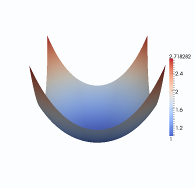
(a) The FE approximation to the function $u(\boldsymbol{x})=\exp\!\left({\frac{\left|\boldsymbol{x}\right|^{2}}{2}}\right)$.

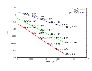
(b) Log–log error plot for $\mathbb{P}^{2}$ Lagrange FEs.

Figure 4. A FE–convexity test for the numerical example given in 3. We plot $\operatorname{det}\boldsymbol{H}[U]$ together with the principle minor of $\boldsymbol{H}[U]$.

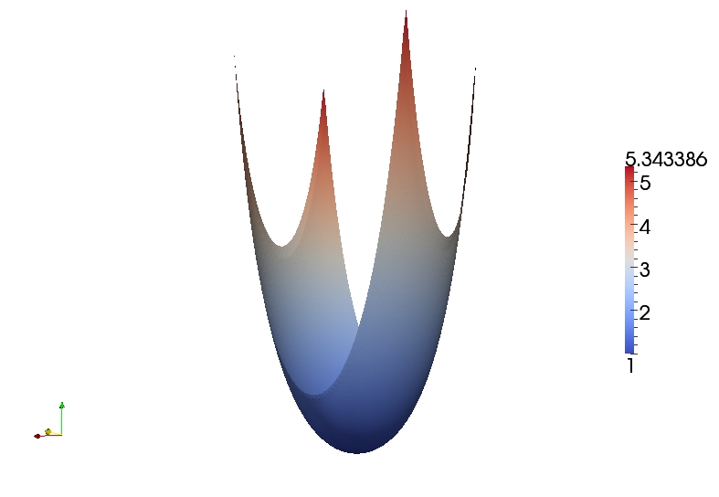
(a) The principal minor of $\boldsymbol{H}[U]$, an approximation to the Hessian of the function $u(\boldsymbol{x})=\exp\!\left({\frac{\left|\boldsymbol{x}\right|^{2}}{2}}\right)$.

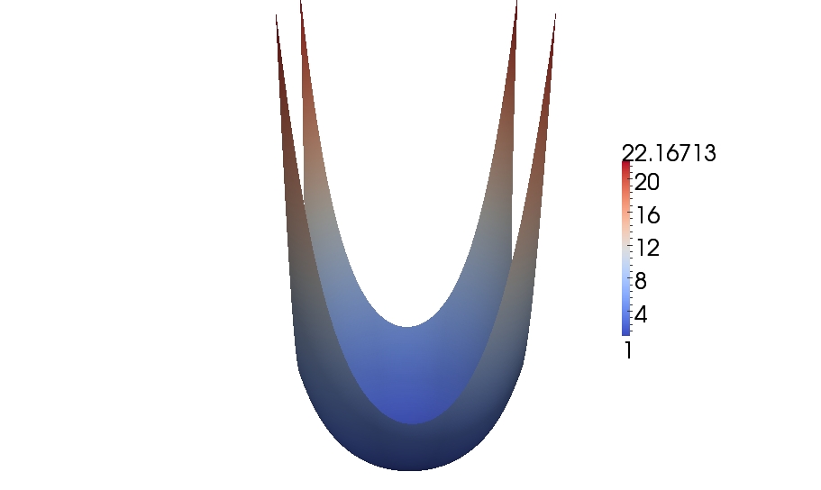
(b) The determinant of $\boldsymbol{H}[U]$.

Figure 5. Numerical results for the MAD problem on the square $S=[-1,1]^{2}$. We choose the problem data $f$ and $g$ appropriately such that the solution is the radially symmetric function $u(\boldsymbol{x})=\exp\!\left({{\left|\boldsymbol{x}\right|^{2}}/{2}}\right)$.

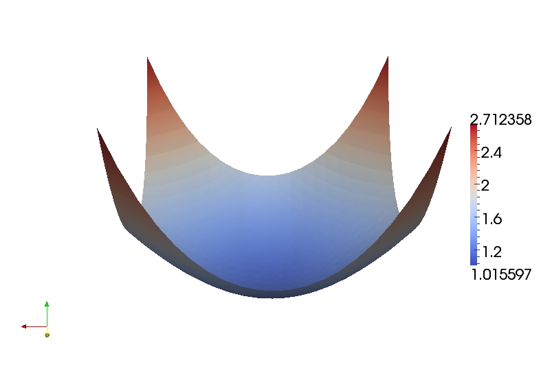
(a) The $\mathbb{P}^{1}$ FE approximation to the function $u(\boldsymbol{x})=\exp\!\left({\frac{\left|\boldsymbol{x}\right|^{2}}{2}}\right)$.

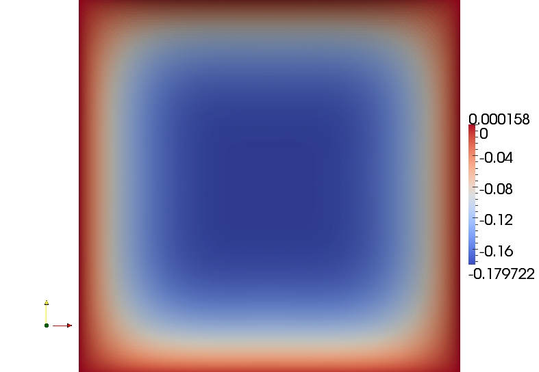
(b) The error $u-U$ plotted as a function over $\varOmega$. Note the FE approximation does not converge in this case, see Remark 5.6

Figure 6. Numerical results for the MAD problem on the square $S=[-1,1]^{2}$. Choosing $f$ and $g$ appropriately such that the solution is $u(\boldsymbol{x})=-\!\left({2-x_{1}^{2}-x_{2}^{2}}\right)^{1/2}$. Note the function has singular derivatives on the corners of $S$. We plot the finite element solution together with a log–log error plot for various error functionals as in Figure 1.

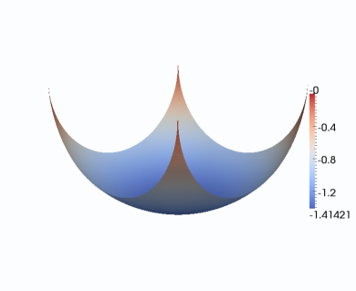
(a) The FE approximation to the function $u(\boldsymbol{x})=-\!\left({2-x_{1}^{2}-x_{2}^{2}}\right)^{1/2}$.

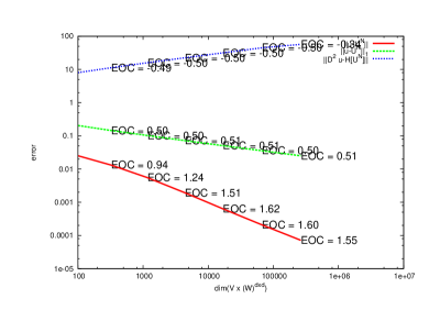
(b) Log–log error plot for $\mathbb{P}^{2}$ Lagrange FEs.

5.7. Nonclassical solutions

The numerical examples given in Figures 3–6 both describe the numerical approximation of classical solutions to the MAD problem. In the case of Figure 3 $u\in\operatorname{C}^{\infty}(\overline{\varOmega})$ whereas in Figure 6 $u\in\operatorname{C}^{\infty}(\varOmega)\cap\operatorname{C}^{0}(\overline{\varOmega})$. We now take a moment to study less regular solutions, i.e., viscocity solutions which are not classical. In this test we the solution

$$u(\boldsymbol{x})=\left|\boldsymbol{x}\right|^{2\alpha}$$ (5.14)

for $\alpha\in(1/2,3/4)$. The solution $u(\boldsymbol{x})\notin\operatorname{H}^{2}(\varOmega)$. In Figures 7–9 we vary the value of $\alpha$ and study the convergence properties of the method. We note that the method fails to find a solution for $\alpha\leq 1/2$. Finally in Figure 10 we conduct an adaptive experiment based on a gradient recovery aposteriori estimator. The recovery estimator we make use of is the Zienkiewicz–Zhu patch recovery technique see publication1, (Pryer, 2010, §2.4) or (Ainsworth and Oden, 2000, §4) for further details.

Figure 7. Numerical results for the MAD problem on the square $S=[-1,1]^{2}$. Choosing $f$ and $g$ appropriately such that the solution is $u(\boldsymbol{x})=\left|\boldsymbol{x}\right|^{2\alpha}$, with $\alpha=0.55$. Note the function is singular at the origin. We plot the finite element solution together with a log–log error plot for various error functionals as in Figure 1.

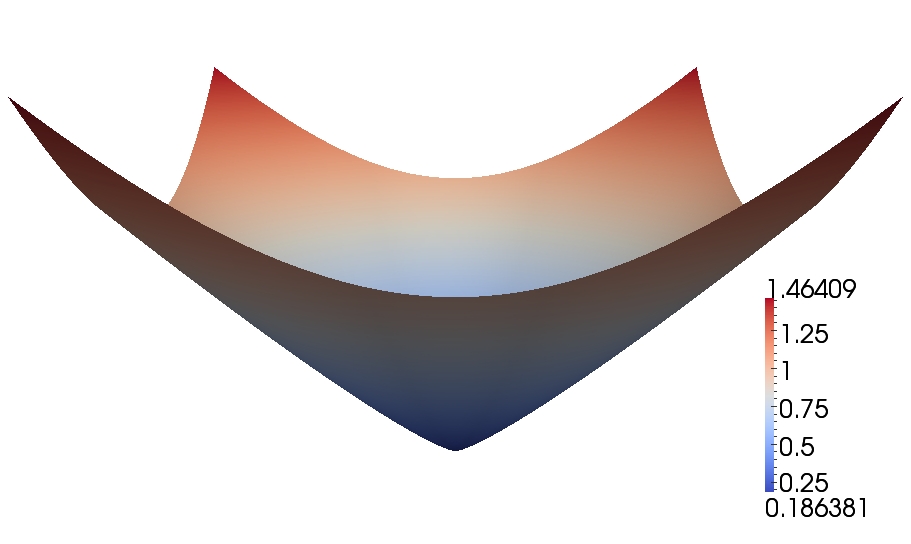
(a) The FE approximation to the function $u(\boldsymbol{x})=\left|\boldsymbol{x}\right|^{2\alpha}$, with $\alpha=0.55$.

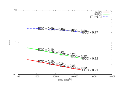
(b) Log–log error plot for $\mathbb{P}^{2}$ Lagrange FEs.

Figure 8. Numerical results for the MAD problem on the square $S=[-1,1]^{2}$. Choosing $f$ and $g$ appropriately such that the solution is $u(\boldsymbol{x})=\left|\boldsymbol{x}\right|^{2\alpha}$, with $\alpha=0.6$. Note the function is singular at the origin. We plot the finite element solution together with a log–log error plot for various error functionals as in Figure 1.

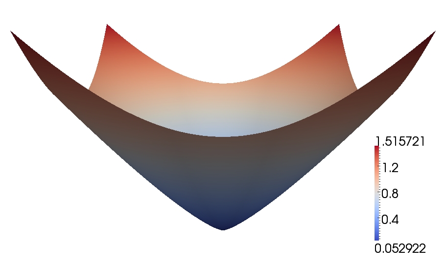
(a) The FE approximation to the function $u(\boldsymbol{x})=\left|\boldsymbol{x}\right|^{2\alpha}$, with $\alpha=0.6$.

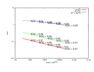
(b) Log–log error plot for $\mathbb{P}^{2}$ Lagrange FEs.

Figure 9. Numerical results for the MAD problem on the square $S=[-1,1]^{2}$. Choosing $f$ and $g$ appropriately such that the solution is $u(\boldsymbol{x})=\left|\boldsymbol{x}\right|^{2\alpha}$, with $\alpha=0.7$. Note the function is singular at the origin. We plot the finite element solution together with a log–log error plot for various error functionals as in Figure 1.

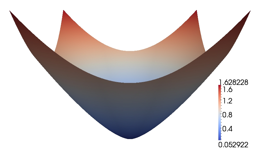
(a) The FE approximation to the function $u(\boldsymbol{x})=\left|\boldsymbol{x}\right|^{2\alpha}$, with $\alpha=0.7$.

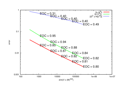
(b) Log–log error plot for $\mathbb{P}^{2}$ Lagrange FEs.

Figure 10. Numerical results for a solution to the Monge–Ampère–Dirichlet equation with $f$ and $g$ appropriately such that the solution is $u(\boldsymbol{x})=\left|\boldsymbol{x}\right|^{2\alpha}$, with $\alpha=0.55$. We choose $p=2$, and use an adaptive scheme based on Z–Z gradient recovery. The mesh is refined correctly about the origin. Note that when $\dim{\mathbb{V}}=20,420$ the adaptive solution achieves $\left\|u-U^{M}\right\|\approx 0.0078$, the uniform solution given in Figure 7 satisfies $\left\|u-U^{M}\right\|\approx 0.18$ using the same number of degrees of freedom. Using the adaptive strategy both $\left\|u-U^{M}\right\|$ and $\left|u-U^{M}\right|_{1}$ converge like $\operatorname{O}(N^{-1})$.

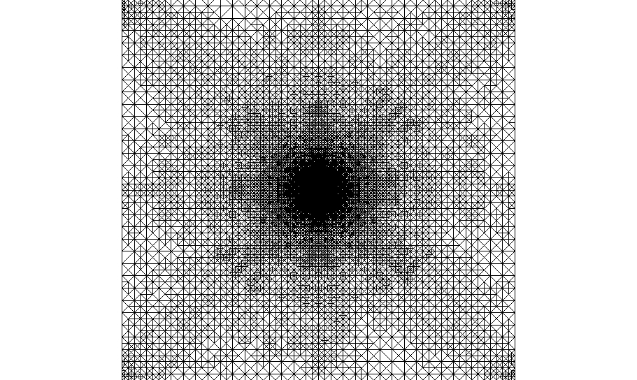
(a) Adaptive mesh

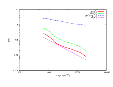
(b) Log–log error plot for $\mathbb{P}^{2}$ Lagrange FEs.

6. Pucci’s equation

In this section we look to discretise the nonlinear problem, in this case Pucci’s equation as a system of nonlinear equations. Pucci’s equation arises as a linear combination of Pucci’s extremal operators. It can nevertheless be written in an algebraically accessible form, without the need to compute the eigenvalues.

6.1. Definition (Pucci’s extremal operators Caffarelli and Cabré (1995))

Let $\boldsymbol{N}\in\operatorname{Sym}{(\mathbb{R}^{d\times d})}$ and $\sigma\!\left({\boldsymbol{N}}\right)$ be it’s spectrum, then the extremal operators are

$$\mathscr{M}(\boldsymbol{N}):=\sum_{\lambda_{i}\in\sigma(\boldsymbol{N})}\alpha_{i}\lambda_{i}=0,$$ (6.1)

with $\alpha_{i}\in\mathbb{R}$. The maximal (minimal) operator, commonly denoted $\mathscr{M}^{+}$ ($\mathscr{M}^{-}$), has coefficients that satisfy

$$0<\alpha_{1}\leq\dots\leq\alpha_{n}\qquad\!\left({\alpha_{1}\geq\dots\geq\alpha_{n}>0}\right)$$ (6.2)

respectively.

6.2. The planar case and uniform ellipticity

In the case $d=2$ the normalised Pucci’s equation reduces to finding $u$ such that

$$\alpha\lambda_{2}+\lambda_{1}=0$$ (6.3)

where $\boldsymbol{N}:=\,\mathrm{D}^{2}u$. Note that if $\alpha=1$ (6.3) reduces to the Poisson–Dirichlet problem. This can be easily seen when reformulating the problem as a second order PDE Dean and Glowinski (2005). Making use of the characteristic polynomial, we see

$$\begin{split}\lambda_{i}=\frac{\Delta u\pm\!\left({\!\left({\Delta u}\right)^{2}-4\operatorname{det}\,\mathrm{D}^{2}u}\right)^{1/2}}{2}\qquad i=1,2.\end{split}$$ (6.4)

Thus Pucci’s equation can be written as

$$0=\!\left({\alpha+1}\right)\Delta u+\!\left({\alpha-1}\right)\!\left({\!\left({\Delta u}\right)^{2}-4\operatorname{det}\,\mathrm{D}^{2}u}\right)^{1/2},$$ (6.5)

which is a nonlinear combination of Monge–Ampère and Poisson problems. However owing to the Laplacian terms, and unlike the Monge–Ampère–Dirichlet problem, Pucci’s equation is (unconditionally) uniformly elliptic for

$$\!\left({\operatorname{tr}{\boldsymbol{X}}}\right)^{2}-4\operatorname{det}\boldsymbol{X}\geq 0\quad\>\forall\>\boldsymbol{X}\in\mathbb{R}^{2\times 2}.$$ (6.6)

The discrete problem we use is a direct approximation of (6.5), we seek $\!\left({U,\boldsymbol{H}[U]}\right)$ such that

$$\int_{\varOmega}\bigg{(}\!\left({\alpha+1}\right)\operatorname{tr}{\boldsymbol{H}[U]}+\!\left({\alpha-1}\right)\!\left({\!\left({\operatorname{tr}{\boldsymbol{H}[U]}}\right)^{2}-4\operatorname{det}\boldsymbol{H}[U]}\right)^{1/2}\bigg{)}\Phi=0$$ (6.7)

$$\left\langle{\boldsymbol{H}[U],\Psi}\right\rangle=-\int_{\varOmega}{\nabla U}\otimes{\nabla\Psi}+\int_{\partial\varOmega}{\nabla U}\otimes{\boldsymbol{n}\ \Psi}\quad\>\forall\>(\Phi,\Psi)\in\mathring{\mathbb{V}}\times\mathbb{V}.$$ (6.8)

The result is a nonlinear system of equations which was solved using a algebraic Newton method.

6.3. Numerical experiments

We conduct numerical experiments to be compared with those of Dean and Glowinski (2005). The first problem we consider is a classical solution of Pucci’s equation (6.3). Let $\boldsymbol{x}={\!\left({x,y}\right)}^{{\boldsymbol{\intercal}}}$, then the function

$$u(\boldsymbol{x})=-\!\left({\!\left({\!\left({x+1}\right)^{2}+\!\left({y+1}\right)^{2}}\right)^{\!\left({1-\alpha}\right)/2}}\right)$$ (6.9)

solves Pucci’s equation almost everywhere away from $(x,y)=(-1,-1)$ with $g:=u|_{\partial\varOmega}$. Let $\mathscr{T}$ be an irregular triangulation of $\varOmega=[-0.95,1]^{2}$. In Figure 11 we detail a numerical experiement considering the case $\alpha\in[2,5]$.

Figure 11. Numerical results for a classical solution to Pucci’s equation (6.9). As with the case of the MAD problem we choose $p=2$. We use a Newton method to solve the algebraic system until the residual of the problem (see (Kelley, 1995, c.f.)) is less than $10^{-10}$ (which is overkill to minimise Newton error effects). We plot log–log error plots with experimental orders of convergence, for various norms and values of $\alpha$.

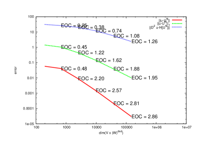
(a) $\alpha=2$

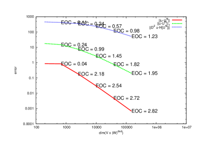
(b) $\alpha=3$

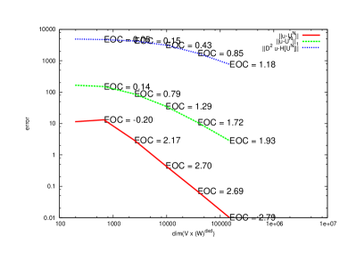
(c) $\alpha=4$

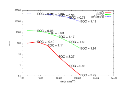
(d) $\alpha=5$

We also conduct a numerical experiment to be compared with Oberman (2008). In this problem we consider a solution of Pucci’s equation with a piecewise defined boundary. Let $\varOmega=[-1,1]^{2}$ and the boundary data be given as

$$g(\boldsymbol{x}):=\begin{cases}1\qquad\text{ when }\left|x\right|\geq\frac{1}{2}\text{ and }\left|y\right|\geq\frac{1}{2}\\ 0\qquad\text{ otherwise.}\end{cases}$$ (6.10)

Figure 12 details the numerical experiment on this problem with various values of $\alpha$.

Figure 12. Numerical results for a solution to Pucci’s equation with a piecewise defined boundary condition (6.10). We choose $p=2$, use a Newton method to solve the algebraic system until the residual of the problem is less than $10^{-10}$. We plot the solution for various values of $\alpha$ as well as a cross section through the coordinate axis. Notice that the solution becomes extremely badly behaved as $\alpha$ increases.

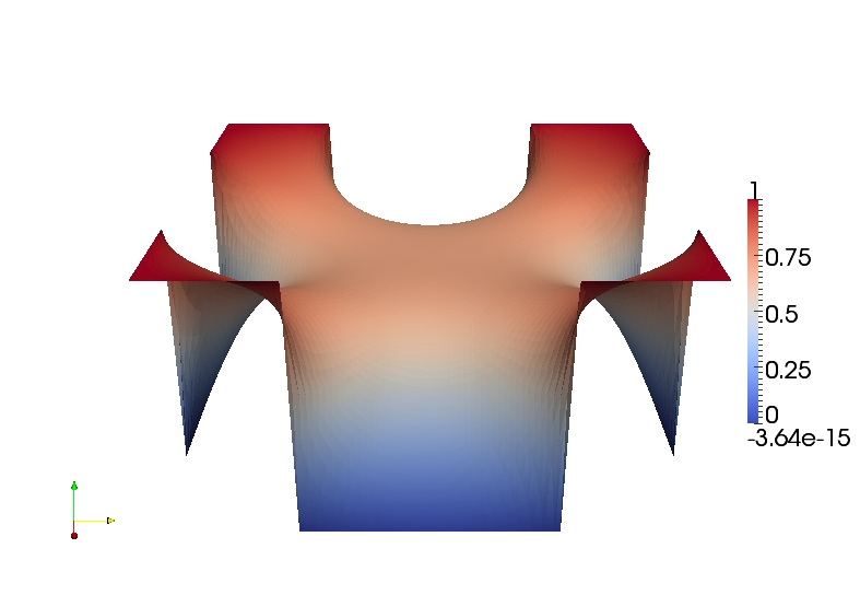
(a) $\alpha=2$

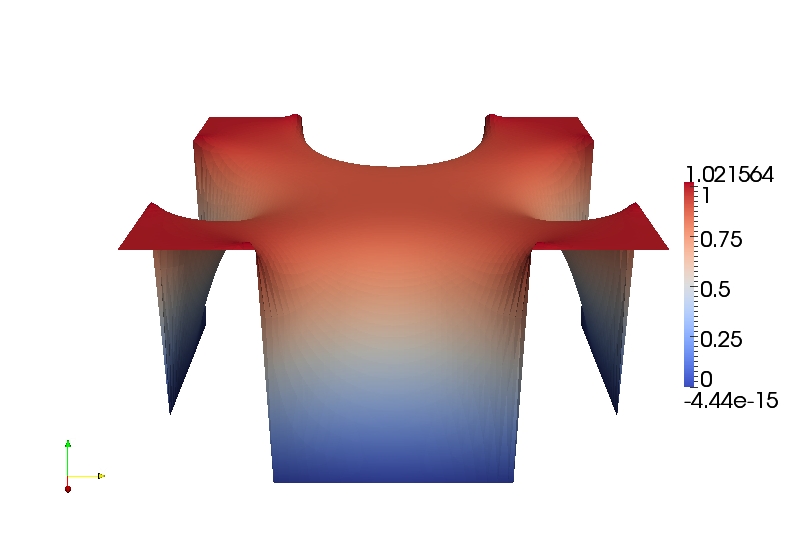
(b) $\alpha=3$

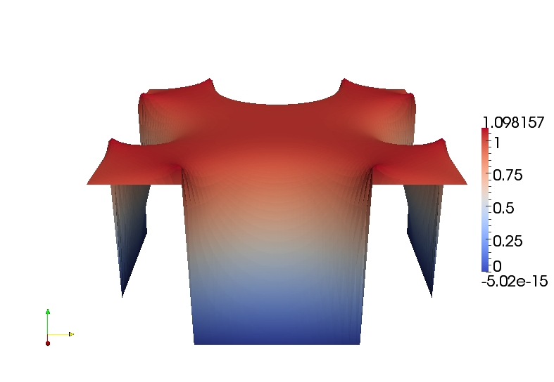
(c) $\alpha=4$

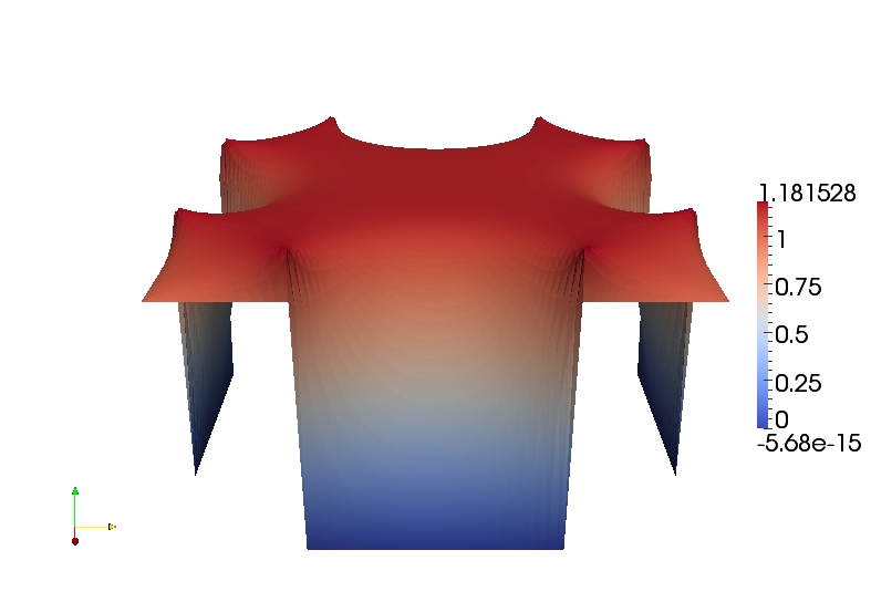
(d) $\alpha=5$

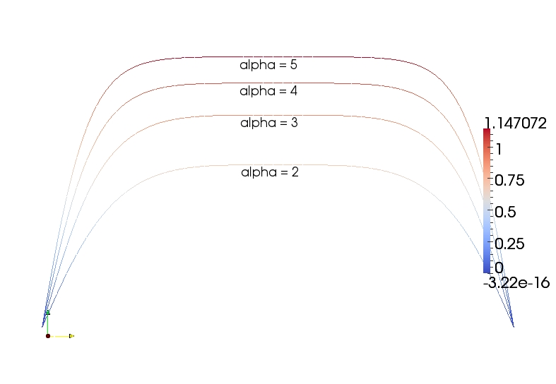
(e) Cross section about $x=0$ for each value of $\alpha$.

Since the solution to the Pucci’s equation with piecewise boundary (6.10) is clearly singular near the discontinuities we have also conducted an adaptive experiment based on a gradient recovery aposteriori estimator (as in §5.7). As can be seen from Figure 13 we regain qualitively similar results using far fewer degrees of freedom.

Figure 13. Numerical results for a solution to Pucci’s equation with a piecewise defined boundary condition (6.10). We choose $p=2$, and use an adaptive scheme based on Z–Z gradient recovery. The mesh is refined correctly about the jumps on the boundary.

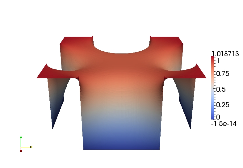
(a) Finite element solution for $\alpha=3$

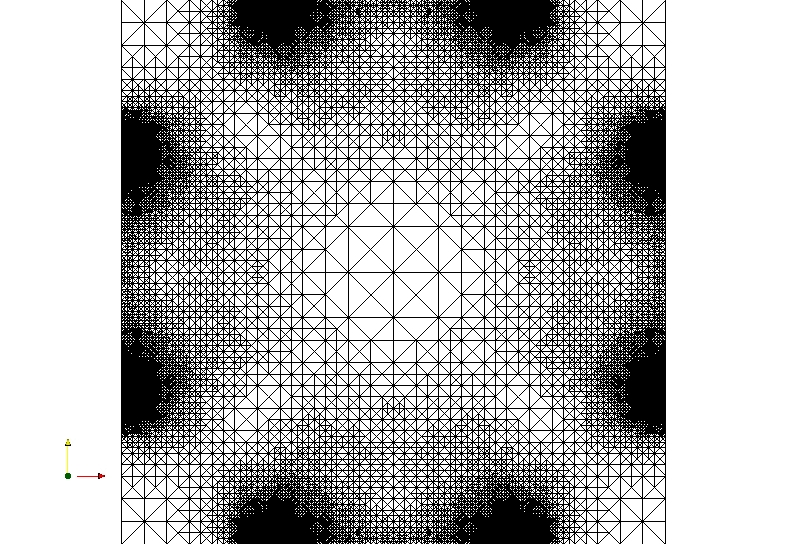
(b) Adaptive mesh

7. Conclusions and outlook

In this work we have proposed a novel numerical scheme for fully nonlinear and generic quasilinear PDEs. The scheme was based on a previous work for nonvariational PDEs (those given in nondivergence form) Lakkis and Pryer (2011).

We have illustrated the application of the method for a simple, non physically motivated example, moving on to more interesting problems, that of the Monge–Ampère equation and Pucci’s equation.

For Pucci’s equation we numerically showed convergence and conducted experiments which may be compared with previous numerical studies.

We demonstrated for classical solutions to the Monge–Ampère equation the method is robust again showing numerical convergence. For less regular viscocity solutions we have found that the method must be augmented with a penalty term in a similar light to Brenner et al. (2011b).

We postulate that the method is better suited to a discontinuous Galerkin framework which is the subject of ongoing research.

References

- Aguilera and Morin [2009] N. E. Aguilera and P. Morin. On convex functions and the finite element method. SIAM J. Numer. Anal., 47(4):3139–3157, 2009. ISSN 0036-1429. doi: 10.1137/080720917. URL http://dx.doi.org/10.1137/080720917.
- Ainsworth and Oden [2000] M. Ainsworth and J. T. Oden. A posteriori error estimation in finite element analysis. Pure and Applied Mathematics (New York). Wiley-Interscience [John Wiley & Sons], New York, 2000. ISBN 0-471-29411-X.
- Awanou [2010] G. Awanou. Spline element method for the Monge–Ampère equation. online preprint, Northern Illinois University, 2010. URL http://www.math.niu.edu/~awanou/SplineMonge7.pdf.
- Awanou [2011] G. Awanou. Pseudo time continuation and time marching methods for Monge–Ampère type equations. online preprint, January 2011. URL http://www.math.niu.edu/~awanou/MongePseudo05.pdf.
- Böhmer [2008] K. Böhmer. On finite element methods for fully nonlinear elliptic equations of second order. SIAM J. Numer. Anal., 46(3):1212–1249, 2008. ISSN 0036-1429. doi: 10.1137/040621740. URL http://dx.doi.org/10.1137/040621740.
- Brenner et al. [2011a] S. C. Brenner, T. Gudi, M. Neilan, and L.-y. Sung. penalty methods for the fully nonlinear monge-ampère equation. Math. Comp., 80:1979–1995, March 2011a. doi: 10.1090/S0025-5718-2011-02487-7.
- Brenner et al. [2011b] S. C. Brenner, T. Gudi, M. Neilan, and L.-y. Sung. penalty methods for the fully nonlinear Monge-Ampère equation. Math. Comp., 80(276):1979–1995, 2011b. ISSN 0025-5718. doi: 10.1090/S0025-5718-2011-02487-7. URL http://dx.doi.org/10.1090/S0025-5718-2011-02487-7.
- Caffarelli and Cabré [1995] L. A. Caffarelli and X. Cabré. Fully nonlinear elliptic equations, volume 43 of American Mathematical Society Colloquium Publications. American Mathematical Society, Providence, RI, 1995. ISBN 0-8218-0437-5.
- Ciarlet [1978] P. G. Ciarlet. The finite element method for elliptic problems. North-Holland Publishing Co., Amsterdam, 1978. ISBN 0-444-85028-7. Studies in Mathematics and its Applications, Vol. 4.
- Davydov and Saeed [2010] O. Davydov and A. Saeed. Stable splitting of bivariate splines spaces by bernstein-bézier methods. online preprint, University of Strathclyde, Department of Mathematics and Statistics, University of Strathclyde, Glasgow, Scotland GB, 11 2010. URL http://personal.strath.ac.uk/oleg.davydov/stable_splBB.html. to appear on LNCS.
- Davydov and Saeed [2012] O. Davydov and A. Saeed. Numerical solution of fully nonlinear elliptic equations by Böhmer’s method. Technical report, University of Strathclyde, 26 Richmond Street, Glasgow GB-G1 1XH, Scotland, UK, January 2012. URL http://personal.strath.ac.uk/oleg.davydov/fully_nonlin.html.
- Dean and Glowinski [2003] E. J. Dean and R. Glowinski. Numerical solution of the two-dimensional elliptic Monge-Ampère equation with Dirichlet boundary conditions: an augmented Lagrangian approach. C. R. Math. Acad. Sci. Paris, 336(9):779–784, 2003. ISSN 1631-073X.
- Dean and Glowinski [2005] E. J. Dean and R. Glowinski. On the numerical solution of a two-dimensional Pucci’s equation with Dirichlet boundary conditions: a least-squares approach. C. R. Math. Acad. Sci. Paris, 341(6):375–380, 2005. ISSN 1631-073X.
- Dean and Glowinski [2006] E. J. Dean and R. Glowinski. Numerical methods for fully nonlinear elliptic equations of the Monge-Ampère type. Comput. Methods Appl. Mech. Engrg., 195(13-16):1344–1386, 2006. ISSN 0045-7825.
- Evans [1998] L. C. Evans. Partial differential equations, volume 19 of Graduate Studies in Mathematics. American Mathematical Society, Providence, RI, 1998. ISBN 0-8218-0772-2.
- Feng and Neilan [2009a] X. Feng and M. Neilan. Mixed finite element methods for the fully nonlinear Monge-Ampère equation based on the vanishing moment method. SIAM J. Numer. Anal., 47(2):1226–1250, 2009a. ISSN 0036-1429. doi: 10.1137/070710378. URL http://dx.doi.org/10.1137/070710378.
- Feng and Neilan [2009b] X. Feng and M. Neilan. Vanishing moment method and moment solutions for fully nonlinear second order partial differential equations. J. Sci. Comput., 38(1):74–98, 2009b. ISSN 0885-7474. doi: 10.1007/s10915-008-9221-9. URL http://dx.doi.org/10.1007/s10915-008-9221-9.
- Froese [2011] B. D. Froese. A numerical method for the elliptic monge-ampère equation with transport boundary conditions. Technical report, 01 2011. URL http://arxiv.org/abs/1101.4981v1.
- Jensen and Smears [2012] M. Jensen and I. Smears. Finite element methods with artificial diffusion for hamilton-jacobi-bellman equations. Technical report, 01 2012. URL http://arxiv.org/abs/1201.3581v2.
- Kelley [1995] C. T. Kelley. Iterative methods for linear and nonlinear equations, volume 16 of Frontiers in Applied Mathematics. Society for Industrial and Applied Mathematics (SIAM), Philadelphia, PA, 1995. ISBN 0-89871-352-8. With separately available software.
- Kuo and Trudinger [1992] H. J. Kuo and N. S. Trudinger. Discrete methods for fully nonlinear elliptic equations. SIAM J. Numer. Anal., 29(1):123–135, 1992. ISSN 0036-1429. doi: 10.1137/0729008. URL http://dx.doi.org/10.1137/0729008.
- Kuo and Trudinger [2005] H.-J. Kuo and N. S. Trudinger. Estimates for solutions of fully nonlinear discrete schemes. In Trends in partial differential equations of mathematical physics, volume 61 of Progr. Nonlinear Differential Equations Appl., pages 275–282. Birkhäuser, Basel, 2005. doi: 10.1007/3-7643-7317-2˙20. URL http://dx.doi.org/10.1007/3-7643-7317-2_20.
- Lakkis and Pryer [2011] O. Lakkis and T. Pryer. A finite element method for second order nonvariational elliptic problems. SIAM J. Sci. Comput., 33(2):786–801, 2011. ISSN 1064-8275. doi: 10.1137/100787672. URL http://dx.doi.org/10.1137/100787672.