Fulde Ferrell Larkin Ovchinnikov oscillations and magnetic domains in the Hubbard model with off-diagonal Coulomb repulsion

Abstract

We observe the effect of non-zero magnetization $m$ onto the superconducting ground state of the one dimensional Hubbard model with off-diagonal Coulomb repulsion $X$. For $t/2\lesssim X\lesssim 2t/3$, the system first manifests Fulde-Ferrell-Larkin-Ovchinnikov oscillations in the pair-pair correlations. For $m=m_{1}$ a kinetic energy driven macroscopic phase separation into low-density superconducting domains and high-density polarized walls takes place. For $m>m_{2}$ the domains fully localize, and the system eventually becomes a ferrimagnetic insulator.

1 Introduction

In the century-long search for a mechanism which unveils the origin of superconductivity in so many different materials, a key ingredient is to understand the role of magnetic correlations in the formation of the superconducting (SC) pairs. Apart form the Meissner effect, different magnetic effects have been described in superconductors, such as the ferromagnetic to superconductor transition in heavy fermions compounds[1], or the magnetic field driven SC-insulator transitions in some two-dimensional high-$T_{c}$ samples[2]. The very recent discovery of high-$T_{c}$ superconductivity in iron based layered pnictides [3], and the observation of coexisting micro- and/or mesoscopic SC and magnetically ordered domains[4, 5] which are reminiscent of the stripes characteristic of cuprates, confirms the suggestion that superconducting and magnetic order are intimately related, and can be crucial for each other’s stability [6]. On the theoretical side, it has also been predicted that SC correlations in presence of non-zero magnetization can rearrange their spatial modulation exhibiting Fulde-Ferrell-Larkin-Ovchinnikov(FFLO) oscillations [7], which are expected in case of strongly anisotropic (for instance one-dimensional) systems. It is a remarkable very recent achievement their observation in both heavy fermions systems and one dimensional Fermi gases[9, 8].

It is generally accepted that the above behaviours are to be ascribed to the presence of electronic correlations in the different systems. The reference model to deal with electron-electron interaction on lattices is given by the Hubbard Hamiltonian, in which the main contribution of the Coulomb repulsion to the model Hamiltonian is identified with the on-site interaction of electrons with opposite spins ($U$ term). The presence of a SC phase at $U>0$ for this model is still matter of debate, though some encouraging results have been achieved (see for instance [10] and the discussion therein). Many extensions of the Hubbard model have been proposed, based on the inclusion of the first contributions to the Coulomb repulsion other than the $U$ term. Among them, a generalization motivated independently by Hirsch[11] and Gammel and Campbell [12] amounts to include the nearest neghbors off-diagonal interaction $X$, which turns out to modulate the hopping term depending on the occupations of the two sites. In this case, the model Hamiltonian reads

$$H=-\sum_{<i,j>\sigma}[1-x\>(n_{i\bar{\sigma}}+n_{j\bar{\sigma}})]c_{i\sigma}^{\dagger}c_{j\sigma}+u\sum_{i}n_{i\uparrow}n_{i\downarrow}+h\sum_{i}(n_{i\uparrow}-n_{i\downarrow})\;$$ (1)

where $c_{i\sigma}^{\dagger}$ creates a fermion with spin $\sigma=\{\uparrow,\downarrow\}$, $\bar{\sigma}$ denoting the opposite of $\sigma$, $n_{i\sigma}=c_{i\sigma}^{\dagger}c_{i\sigma}$ is the $\sigma$-electron charge and $\langle ij\rangle$ stands for nearest-neighboring sites. The parameters $u$ and $x$ are the dominant diagonal and off-diagonal contribution coming from Coulomb repulsion, and the lower case symbols denote that these coefficients have been normalized in units of the hopping amplitude. Here we have also included an external magnetic field $h$. Moreover, $N$ is the number of electrons on the $d$-dimensional $L$-sites lattice, so that $n=N/L$ is the average filling value per site. The model has been extensively studied in the literature at $h=0$ [13]. In particular, since $H$ is not invariant under particle-hole transform, it has been proposed to model a theory of hole superconductivity.[11]
While the effect of the off-diagonal Coulomb repulsion (also known as bond-charge interaction) has long be disregarded since it is usually smaller than the diagonal contributions of Coulomb interaction (Hubbard and extended Hubbard models), it has by now become clear that what matter is instead its amplitude compared with that of the hopping term. In fact already for $x\gtrsim 1/2$ a scenario quite different from that of the Hubbard limit emerges [14, 15] even in $d=1$. In particular, for not too large on-site Coulomb repulsion $u<u_{c}(x)$ a new metallic phase appears, characterized by dominant SC correlations and nanoscale phase separation[16] (NPS). The latter amounts to the coexistence of two conducting phases with different densities[17], and is driven by the charge degrees of freedom. The actual size of the coexisting domains turns out to be microscopic at $h=0$, and to increase in relation to the imbalance in spin orientation[18], suggesting an interplay of charge and spin degrees of freedom in the ground state. Since none of the two coexisting phases is separately SC, it is reasonable to interpret this emergent SC behaviour as a consequence of the microscopic domain size induced, in turn, by spin rearrangement; we are in presence of magnetic mediated superconductivity. A further confirmation of this hypothesis comes from a very recent result [19] which shows that the critical line for the SC transition can be recovered exactly (see figure 1, left panel) if assuming short range antiferromagnetic correlations between just the single electrons. It must be noticed that the appearance of antiferromagnetic and metallic behaviour at half-filling, in a regime of moderate interaction, as well as its interplay with SC properties, is somehow reminiscent of the physics characterizing iron pnictides in higher dimension.

To better understand the role of magnetic correlations in ground-state of Hamiltonian (1) and their interplay with the charge degrees of freedom, here we shall investigate –through a detailed density-matrix renormalization group (DMRG) numerical study [20]– the consequences of the inclusion of the magnetic field as to the onset of the SC phase. In principle, increasing the magnetic field should force the spin degrees of freedom to align to the external field, so that the underlying phase separation (PS) in the charge degrees of freedom should emerge at a macroscopic level, wiping out the SC properties. In fact, what we will see is that the SC pairs can survive even at non-zero magnetization, acquiring a modulation of FFLO type [7]. For higher values of the external field however, the density domain texture of the ground state emerges, and the SC pairs become first confined to the low density domains only, while the high density domains behave as polarized walls. Finally, above an upper value of the magnetic field superconductivity disappears and the ferromagnetic domains localize: the system becomes a ferrimagnetic insulator.

In section II we describe some features of the model Hamiltonian, investigating in particular the role of the kinetic energy as to the onset of the different transitions. In section III we investigate the static spin and charge structure factor dependence on the magnetization. The study of the Luttinger charge ($K_{\rho}$) and spin ($K_{\sigma}$) parameters allows to identify the presence of superconducting metallic and insulating phase. In section IV we explore the spatial dependence of density and magnetization with increasing the magnetic field. In section V we study the dependence of various type of pair-pair correlations and give evidence of the related emergence of FFLO oscillations. Finally in section VI we discuss the results and give some conclusions.

2 The bond-charge Hubbard model

2.1 Phase diagram at $h=0$

The ground-state phase diagram of Hamiltonian (1) at $h=0$, as obtained numerically in [14, 15, 16, 19] is reported in figure 1. On the left-hand side this is given at fixed filling ($n=1$) and varying $u>0$, $x$, whereas on the right-hand side it is given at $u=1$, varying $n$ and $x$. Various phases can be recognized: in particular a Luther-Emery liquid phase [21] with dominant superconducting correlations (SC) takes place in a range of filling values which depends on $x$. Within such phase, one can distinguish three different regimes:

• (i)For $0<x\lesssim 1/2$ the transition to the SC phase possibly takes place for $n>1$ and not too large $u$ as soon as $x\neq 0$, in agreement with bosonization predictions [22] (not shown).

• (ii) For $1/2\lesssim x\lesssim 2/3$ we are in an intermediate regime. The SC phase still appears for $0<u\leq u_{c}(x,n)$ in a wider range $n_{l}\leq n\leq 2$ with $n_{l}\leq 1$.

• (iii)For $2/3\lesssim x\leq 1$ nanoscale PS (NPS) is observed in the SC phase as a texture of two fluids of different densities $n_{l}$ and $n_{h}$, which coexist up to $u_{c}(x,n)$ for a range of filling values $n_{l}\leq n\leq n_{h}<2$, with $n_{l}\leq 1$.

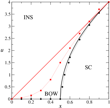
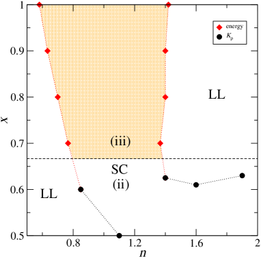
Figure 1: Ground state phase diagram of $H$ in one dimension (in the absence of external magnetic field). INS denotes the insulating phase, LL denotes the phase described by a Luttinger Liquid while BOW denotes the phase supporting bond order (charge density) wave [21]. Symbols (with joining dots) denote numerical results. Left panel: half-filling; continuous lines denote the analytical expressions for the critical lines obtained in [19]. Right panel: $u=1$ (the legend refers to the methods used in [16] to locate the transition points). Dashed line marks $x=2/3$.

2.2 Role of kinetic energy

The crossover among the above different regimes can be observed for instance on the ground-state energy $e_{gs}$, plotted in figure 2(left) at half-filling and $u=0$ versus $x$. With increasing $x$, $e_{gs}$ turns out to increase linearly from the value $e_{k}(x=0)=-4/\pi$ (non interacting electrons with spin) to the value $e_{k}\approx-2/\pi$ reached for $x=1/2$, in agreement with bosonization predictions. Being the latter coincident with the energy of a system of spinless fermions at quarter filling, from this point on the system becomes unstable with respect to PS into two regions at different densities (approximately $1/4$ and $3/4$) in region (ii), and correspondingly $e_{gs}$ is seen to deviate from the linear increasing, reaching its maximum for $x\approx 2/3$. Above such value, the system enters region (iii), and the ground-state energy begins to decrease, to gain the value $-2/\pi$ precisely at $x=1$. At this point the system can be regarded either as describing a fluid of spinless fermions moving in a background of empty and doubly occupied sites[23], or as two coexisting fluids of single electrons moving in a background of empty and doubly occupied sites [17], in which case $n_{l}=0.5$ and $n_{h}=1.5$.

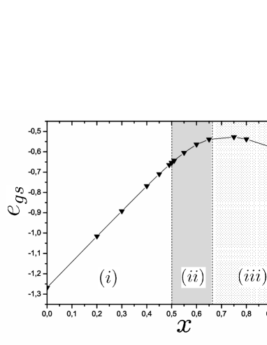
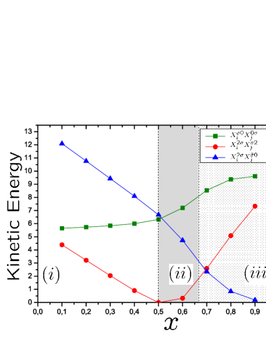
Figure 2: The case of vanishing magnetization at half-filling, $u=0$. Left: Ground-state energy vs $x$. Right: the three contribution to kinetic energy in (2) plotted vs $x$. In both cases the three different regions (with white, gray, and dotted background) correspond to the three different behaviour described in section 1: Hubbard-like, SC, NPS.

The significance of the points $x=1/2$ and $x=2/3$ at $u=0$ becomes evident when representing the Hamiltonian in terms of on-site Hubbard projectors, which are operators defined as $X_{i}^{\alpha\beta}\doteq|\alpha\rangle_{i}\langle\beta|_{i}$. Here $|\alpha\rangle_{i}$ are the states allowed at a given site $i$, and $\alpha=\{0,\uparrow,\downarrow,2\}$ [$|2\rangle\equiv|\uparrow\downarrow\rangle$]. In this case the nonvanishing entries of the Hamiltonian matrix representation are read directly as the nonvanishing coefficients of the projection operators. When rewritten in terms of these operators, $H$ turns out to be a subcase of the more general Hamiltonian introduced by Simon and Aligia,[24]

$$H_{BC}=-\sum_{<ij>\sigma}\left[X_{i}^{\sigma 0}X_{j}^{0\sigma}+t_{x}X_{i}^{2\sigma}X_{j}^{\sigma 2}+s_{x}(X_{i}^{\sigma 0}X_{j}^{\bar{\sigma}2}-X_{i}^{2\sigma}X_{j}^{0\bar{\sigma}})\right]+u\sum_{i}X_{i}^{22}$$ (2)

in which $t_{x}=1-2x$ and $s_{x}=1-x$. Besides $u$, the behaviour of $H_{BC}$ is determined by the strength of $t_{x}$ and $s_{x}$. In particular, $x=1/2$ implies $t_{x}=0$, whereas below and above such value $t_{x}$ changes sign. A negative $t_{x}$ induces frustration in the motion of pairs, since it favors the presence in the ground state of momenta close to zero. A positive $s_{x}$ term instead drives the pairs hopping favoring the modes with momenta close to the edge of the Brillouin zone. Hence we expect that for $|t_{x}|\gtrsim|s_{x}|$ –in our case $x\gtrsim 2/3$– the mobility of the pairs becomes favored in the system for $u\leq u_{c}(x)$. This is summarized in the right-hand side of figure 2, where the three contributions to the kinetic energy in (2) are plotted separately at $u=0$. It is seen that in the three regions the relative weights of these contributions to the total kinetic energy are ordered in different ways. In particular, while at $x\leq 1/2$ the term with coefficient $s_{x}$, which does not conserve the number of pairs, plays the dominant role, for $x\geq 1/2$ this role is taken by the term describing the mobility of single electrons in a background of empty sites (coefficient $1$), conserving the number of doublons; for $x\gtrsim 2/3$ the term with coefficient $s_{x}$ becomes the smallest, to vanish exactly at $x=1$. In practice, a consequence of the above behaviour is that for $x\geq 2/3$ in the ground state the number of pairs is conserved, and the fluid behaves as a system of $N_{s}$ single electrons moving in a background of $L-N_{s}$ empty and doubly occupied sites. This is shown for instance in the charge structure factor $N(q)=\sum_{i}(\langle n_{i}n_{i+r}\rangle-\langle n_{i}\rangle\langle n_{i+r}\rangle){\rm{e}}^{{\rm{i}}qr}$, which correspondingly manifests a feature at $q=2\pi N_{s}/L$

The reasons for the further choice of NPS, with respect to macroscopic PS, are to be found in the behaviour of the spin degrees of freedom, and their interplay with charge degrees of freedom. Indeed the term with coefficient $s_{x}$ tends to favor antiferromagnetism at short range in an appropriate background of empty and doubly occupied sites. It is the surprising result of a very recent paper [19] that this simple assumption allows to map the Hamitonian in the SC regime into an effective XY model in a transverse field, recovering the critical line shown in figure 1 as the factorization line of the XY model. Remarkably, such line is not critical in the XY model: it is just the coupling of it to the charge degrees of in the original model which determines a change of phase.

2.3 Results at $h\neq 0$

At $h\neq 0$ there are results available both at $x=1$[25], which case can be treated exactly also at non-zero temperature, and at $x\neq 1$[26], where the numerical method employed required the presence of a non-vanishing temperature. A low temperature peak in the specific heat, to be ascribed to the excitation of the spin degrees of freedom, is observed for $x\leq 1/2$ already at vanishing field, and at non-vanishing field for $x\lesssim 1$.
Also, numerical results at $T=0$ have been obtained more recently for imbalanced species of ultracold fermionic atoms, both in case of attractive [27], and in case of repulsive [18] $u$. In this latter case it was realized that a non-trivial consequence of the phase coexistence in region (iii) is that within the NPS phase the number of pairs $n_{d}$ is constant with increasing $m$, up to a critical magnetization $m_{c}=n-n_{\downarrow}=n-2n_{d}$ at which the doublons begin to break, entering a regime of breached pairs. This is shown by the numerical data reported in figure 3, where also the analytical value obtained at the same $t_{x}$ values assuming $s_{x}=0$ are reported. It is seen that while in region (iii) the numerical data at $s_{x}=0$ coincide with the theoretical curve already at $m=0$, in the intermediate region (ii) this happens only at large enough values of $m$ ($m>m_{c}$). Also the size of the coexisting domains, microscopic for $h=0$, is observed to become macroscopic at appropriate non-zero magnetization in both regions.

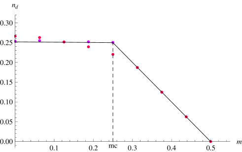
Figure 3: Number of doubly occupied sites versus magnetization at two different values of $x$, inside region (ii) (pink dots) and (iii) (violet dots) respectively. Continuous line is the theoretical prediction at $x=0.8$ ($s_{x}=0$); dashed line is the critical magnetization at which the breached pair regime is entered in that case.

2.4 DMRG simulations

Some observables considered in this work are better studied with periodic boundary conditions, while others are obtained numerically with more precision employing open boundary conditions. In both cases we retained up to 768 optimized DMRG states, performing usually three finite-system sweeps to enforce ground-state convergence. With more than 100 sites, the truncation errors in the density matrix weight remain $O(10^{-6})$ or smaller. As far as the dependence on the system size is concerned, due to the large number of points selected in the phase diagram we decided to report the results for a fixed chain length L=160, unless otherwise specified. However, for some selected points we carried out a preliminar analysis of system size dependence (not reported here) and observed that the behaviour of the various correlation functions was essentially the same at different values of (sufficiently large) L. Moreover, due to the onset of PS for some parameters value (see below), it could be difficult to reproduce the same qualitative spatial pattern by varying the system size. Hence the data presented at fixed length are chosen to be representative of the physical behaviour seen also at smaller sizes.

3 Luttinger exponents: charge and spin structure factor at $h\neq 0$

We have seen that at non-zero magnetization the structure of the ground state in region (iii) does not change –for what concerns the presence of empty and doubly occupied sites– up to the value $m_{c}$. To some extent, this observation holds even inside region (ii). This is consistent with the possibility that an external magnetic field simply changes the polarization of the single electrons in the ground state. At non zero magnetization however the electrons should arrange differently regarding their pairing property. On general grounds, one of the two following scenarios is expected to hold above a first critical field $h_{c_{0}}$ at which the system begins to magnetize: either the SC properties are lost, or the SC pairs acquire a non-vanishing momentum and FFLO oscillations are observed [7], due to the presence of polarized single electrons which do not pair.

In order to explore what happens to the SC properties of the ground state in the two regions (ii) and (iii) at non-zero magnetization, we first evaluate the static charge $N(q)$ and spin $S(q)$ ($S(q)=\sum_{i}(\langle s_{i}^{(z)}s_{i+r}^{(z)}\rangle-\langle s_{i}^{(z)}\rangle\langle s_{i+r}^{(z)}\rangle){\rm{e}}^{{\rm{i}}qr}$, with $s_{i}^{(z)}\doteq(n_{i\uparrow}-n_{i\downarrow})$) structure factors at different values of the average magnetization $m=1/(2L)\sum_{i}<s_{i}^{(z)}>$. From the low frequency behaviour of these quantities one can extract the spin ($K_{\sigma}$) and charge ($K_{\rho}$) exponents which characterize the possible presence of gapped phases as:

$$K_{\rho}=\frac{\pi}{q}N(q\rightarrow 0)\quad,\quad K_{\sigma}=\frac{\pi}{q}S(q\rightarrow 0)\quad.$$

We recall that at $m=0$ both in region (ii) and (iii) the ground-state is a Luther-Emery SC liquid, i.e. it is characterized by $K_{\sigma}=0$ and $K_{\rho}>1$. The actual values of $K_{\rho}$ for $m>0$ , as obtained from DMRG simulations at two different representative values of $x$, are given in figures 5 and 5 (the latter showing indirectly $K_{\sigma}$ through the slope at $q=0$).

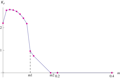
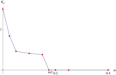
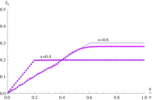
Figure 4: Luttinger exponent (see text) $K_{\rho}$ at $u=0$, $x=0.6$ (region (ii), left), and $x=0.8$ (region (iii), right) as obtained from DMRG simulations (L=160). The two discontinuities identify the critical values $m_{1}$ and $m_{2}$ discussed in the text.

Figure 5: Spin structure factor at high magnetization $m>m_{c}$ ($m=0.4$), for $x=0.4$ and $x=0.6$ as obtained from DMRG simulations ($L=160)$. The crossover from a spinful to a spinless regime is shown: continuous lines represent the theoretical prediction for a spinful fluid at half filling ($x=0.4$); and a spinless fluid of $2m$ fermions ($x=0.6$).

At low enough magnetization, in both regions we still see evidence of a closed charge gap, and an open spin gap (not shown). However, as soon as $m\neq 0$ in region (iii) $K_{\rho}<1$ : the SC correlations are no longer dominant. On the contrary, in region (ii) $K_{\rho}>1$ up to the critical magnetization $m_{1}\approx 0.1$ reported in figure 5. In this case we can conclude that superconductivity is still present in the magnetized ground state. Accordingly to our previous discussion, this should imply the presence of FFLO type of oscillations, which will be investigated in section 5. A further interesting aspect which appears in both regions is the presence of a higher magnetization value $m_{2}$ above which the system appears to become insulating: even at finite size, $K_{\rho}$ is zero within the numerical error. On the other hand our numerical data suggest that within the insulating regime the spin gap remains open until the magnetization reaches the value $m_{c}$ at which the breached pair regime is entered. Whereas for $m>m_{c}$ $K_{\sigma}=1/2$ at variance with the standard Hubbard case in which $K_{\sigma}=1$ (see figure 5). The result is a signal of the fully polarized nature of the single electrons for $m>m_{c}$ in regions (ii) and (iii), which implies that $K_{\sigma}$ coincides with the Luttinger exponent of a gapless spinless liquid, i.e. $1/2$. This is also confirmed by the fact that $S(q)$ manifests a feature at $q=\pi n_{s}$, where $n_{s}$ namely the number of single electrons, coincides for a fully polarize liquid with $n_{\uparrow}-n_{\downarrow}$.

To exploit the nature of the difference between region (ii) and (iii) we also show in figure 6 $S(q)$ for $x=0.6,0.8$ at various magnetization values below $m_{2}$. We recall that in the standard Luttinger liquid case a feature is expected in $S(q)$ for $q=2\pi n_{\sigma}$[29], whereas a signal of the presence of FFLO would be a feature at $Q=2\pi(n_{\uparrow}-n_{\downarrow})$[28].

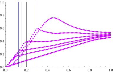
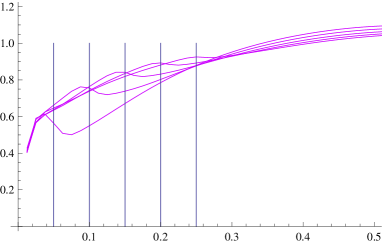
Figure 6: Spin structure factor at various values of magnetization $m\leq m_{2}$. Left panel: $S(q)$ at $x=0.8$, vertical lines in correspondence of $2n_{s\downarrow}$. Right panel: $S(q)/q$ at $x=0.6$, vertical lines in correspondence of $2m$ .

Starting from region (iii), at $x=0.8$ we observe a feature at $q=2\pi n_{s\downarrow}$, which confirms that in this case the behaviour of magnetic correlations in the phase is that of a liquid of $n_{s}$ particle, moving in a background of $n-n_{s}$ empty and doubly occupied sites, in agreement with our previous observations: in this case, it is just the spin degrees of freedom of the $n_{s}$ single electrons which rearrange under the external magnetic field. In region (ii) instead, at $x=0.6$ there is a neat feature at $Q=2\pi(n_{\uparrow}-n_{\downarrow})$, which is a further signal of the presence of FFLO oscillations. Such possibility will be explored in section 5. The feature is strongly reduced for $m\gtrsim m_{1}$. In both regions, the feature disappears at the value $m_{2}$ discussed above.

4 Phase separation and domain formation

Due to quantum superposition and to the microscopic size of the domains, at vanishing magnetic field it is not possible to distinguish directly on the local density $<n(j)>$ and magnetization $<s_{z}(j)>$ profiles the presence of phase coexistence, even in region (iii) where it can easily be detected on the chemical potential [16]. The problem persists at low non-vanishing values of the magnetization, in which case however the local magnetization is observed to display a modulation with wavelength proportional to either $q$ or $Q,$ depending on the value of $x$ and consistently with the behaviour observed in $S(q)$ (see previous section). With further increasing the magnetization, the presence of macroscopic phase separation (MPS) on both the local density and the local magnetization profiles appears well below the critical value $m_{c}$ at which the single electrons become fully polarized. This is seen in figures 7 and 8. In fact, a more careful analysis shows that in region (ii) MPS appears as soon as $m=m_{1}$ (i.e. $K_{\rho}=1$, where the system looses its SC properties) . Whereas in region (iii) MPS can be seen only above the magnetization $m=m_{2}$, in correspondence to the transition to the insulating state. As also shown from the profiles reported in figure 7 in this case the single electrons of the high density domains are fully polarized, and simultaneously the holes are expelled from the same domains, so that the system consists of localized domains with different average magnetization.

In particular, in figure 7 we have chosen to plot separately in region (iii) the site dependence of the number of doubly $<n_{d}(j)>$ , singly occupied $<n_{s\sigma}^{(i)}>$ , and empty $<n_{h}(j)>$ sites in the different regimes. The presence of low and high-density domains can be easily recognized: these consists of spatial regions in which the single electrons move in a background of holes (low density) or doubly occupied (high density) sites, with different Fermi momenta (i.e., in this case different values of $n_{s}=n_{s\uparrow}-n_{s\downarrow}$, shown in figure 7). Since the single electrons can have different spin orientation only in the low density domains, the site magnetization turns out to be constant in the high-density ones, whereas it is modulated according to the number of single electrons with minority spins in the low density domains. The modulation disappears for $m>m_{c}$, when the single electrons become fully polarized along all the system. A consequence of the spatial arrangement is that in the local magnetization profile the low and high density domains may change their relative spin orientation depending on the value of $m$. Indeed, as soon as $m>m_{2}$ the system chooses to lower the magnetization of the low density domains, which weight is more relevant in the kinetic energy. Increasing $m$ then amounts to align more and more spins of the electron in the low density domains, which at $m=m_{2}$ are more numerous than those in the high density domains, so that the relative magnetization is reversed. Recalling that the high and low density domains are characterized respectively by the density of single electrons $n_{sh}$, and $n_{sl}$, in this case it is possible to calculate explicitly $m_{c}$: $m_{c}=n_{sl}-(n_{sh}-1)$.

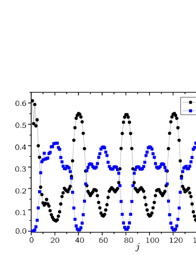
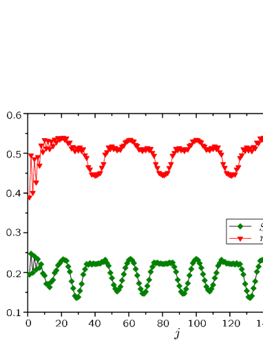
Figure 7: Site dependence of various densities for $x=0.8$ (region (iii)) and $m_{2}\leq m\leq m_{c}$ . Left panel: local densities of holes and of doublons; right panel: local density of single electrons, and magnetization.

As mentioned, in region (ii) it is possible to distinguish the presence of high and low density domains already at lower values of magnetization (figure 8), as soon as SC correlations cease to be dominant in the whole system ($m=m_{1}$). In this case the single electrons with opposite spin orientation vary coherently with the sites in the low density domains, so that their difference (hence the local magnetization) remains constant there. We will see later that this is a further signal of the presence of FFLO in these domains. Whereas the local magnetization appears to be modulated in the high density domains, since the single electrons are not yet fully polarized. The low density phase is different from the one in region (iii), and the coherent behaviour of electrons with opposite spin suggest that in correspondence to the appearance of MPS SC pairs become confined to these domains. Further increasing $m$ above $m_{2}$ the behaviour resembles that of the $x=0.8$ case: in both regions the system behaves de facto as an insulating ferrimagnet.

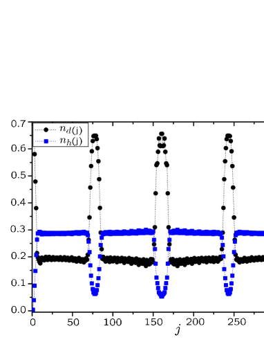
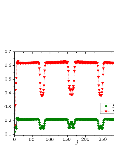
Figure 8: Site dependence of local densities of holes and doubly occupied sites (left panel); single electrons and magnetization (right panel) for $m_{1}\leq m\leq m_{2}$ at $x=0.6$.

Finally for $m>m_{c}$ the breached pairs regime is entered. Again, this fate is shared also by region (ii).

5 Pair-pair correlations and FFLO oscillations

In this section we consider the possible presence of FFLO oscillation in pair pair correlations at non-zero magnetization via the study of various pairing correlators $\langle A_{i}^{\dagger}A_{i+R}\rangle$ where the operator $A_{i}$ at site may refer to $A_{i}^{{\rm onsite}}=\eta_{i}=c_{i\downarrow}c_{i\uparrow}$ (onsite pairing) or to singlet and triplet combinations on adjacent sites $i$ and $i+1$

$$A_{i}^{{\rm sing}}=S_{i}=\frac{1}{\sqrt{2}}(c_{i+1\downarrow}c_{i\uparrow}-c_{i+i\uparrow}c_{i\downarrow})$$

$$A_{i}^{{\rm trip-0}}=T_{0i}=\frac{1}{\sqrt{2}}(c_{i+1\downarrow}c_{i\uparrow}+c_{i+i\uparrow}c_{i\downarrow})$$

$$A_{i}^{{\rm trip}-\sigma}=T_{\pm 1i}=c_{i+1\sigma}c_{i\sigma}\;,\;\;\sigma=\uparrow,\downarrow$$ (3)

For each one of these operators, as well as for their correlators, we can use Hubbard operators $X$ and give a decomposition based on the high-density subspace made only of doubly occupied sites and singly occupied sites ($2\sigma$ elements), the low-density subspace where no doubly occupied sites exist while empty sites are permitted ($0\sigma$ elements). Mixed contributions also must be considered, as can be seen from the example of $T_{1i}=T_{1i}^{{\rm low}}+T_{1i}^{{\rm high}}+T_{1i}^{{\rm mixed}}$ with

$$T_{1i}^{{\rm low}}=X_{i+1}^{0\uparrow}X_{i}^{0\uparrow}\;,\;\;T_{1i}^{{\rm high}}=X_{i+1}^{\downarrow 2}X_{i}^{\downarrow 2}$$

$$T_{1}^{{\rm mixed}}=X_{i+1}^{\downarrow 2}X_{i}^{0\uparrow}+X_{i+1}^{0\uparrow}X_{i}^{\downarrow 2}$$

For $T_{-1i}$ it is sufficient to reverse the index $\sigma$ of single occupation. The 0 component of the triplet and the singlet have similar, although longer, expressions that we do not report here for the sake of brevity.

We discuss the results of a quantitative DMRG analysis by choosing $x=0.6$ and $x=0.8$ as representative parameters of the two somehow different situations of region (ii) and (iii) respectively. All the numerical data presented in this section are taken on chains of $L=120$ with open boundary conditions (OBC) sites at half filling. First, in figure 9 we show evidence of FFLO behaviour showing up when the populations are slightly imbalanced in region (ii). In figure 10, instead, we can see how the FFLO effect is progressively wiped out if either the magnetization density is too high (central panel), or if the interaction $u$ is increased (right panel).

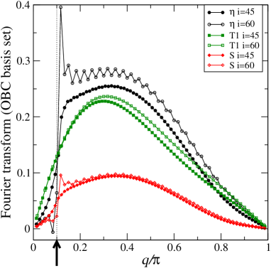
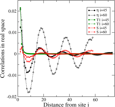
Figure 9: Various types of correlators $\langle A_{i}^{\dagger}A_{i+R}\rangle$ with the choices for $A_{i}$ reported in the legend (compare with (3)). Considering the emerging PS we have selected two possible starting sites $i=45$ or $i=60$. In the left hand side the correlation functions are plotted in reciprocal space and the arrow marks the expected FFLO peak at $q_{{\rm FFLO}}=k_{F\uparrow}-k_{F\downarrow}=\pi(n_{\uparrow}-n_{\downarrow})=2\pi m_{z}$. Here the magnetization density, that allows for the FFLO effect, is $m_{z}=0.05$. The oscillating pattern in real space is evident from the right panel, especially for the dominating $\eta$-pairs correlation that decay slowly. The $T_{1}$ correlations instead do not exhibit the same effect. The model parameters here are $u=0$ and $x=0.6$.

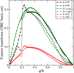
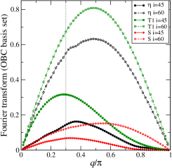
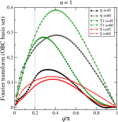
Figure 10: Left and central panel: as figure 9 but with magnetization density increased to $0.1$ and $0.15$ respectively. In the former case a weak signature of FFLO peak remains (it would be expected in correspondence of the dotted vertical line), while in the latter case is wiped out. The same happens by increasing the Coulomb interaction at the same value of $m_{z}=0.1$ (for instance $u=1$ in the example of the right panel).

Due to the possible emergence of PS, that is spatial inhomogeneities, it will be useful to inspect also the variation of the correlators $\langle A_{i}^{\dagger}A_{i+R}\rangle$ along the chain at fixed $R$ as a function of $i$. When $R=1$ there is a site $i+1$ in common between $A_{i}^{\dagger}$ and $A_{i+1}$ (apart from the case $A_{i}=\eta_{i}$) and there are some simplifications in the following correlation functions referred to the “high” and “low” sectors of the Hilbert space

$$\langle T_{\pm i}^{{\rm low}\dagger}T_{\pm i+1}^{{\rm low}}\rangle=-\langle X_{i}^{\sigma 0}n_{s\sigma i+1}X_{i+2}^{0\uparrow}\rangle$$

$$\langle T_{\pm i}^{{\rm high}\dagger}T_{\pm i+1}^{{\rm high}}\rangle=-\langle X_{i}^{2\bar{\sigma}}n_{di+1}X_{i+2}^{\bar{\sigma}2}\rangle$$

where $\pm$ in the subscript corresponds to $\sigma=\uparrow,\downarrow$ and $\bar{\sigma}$ means spin flip. In addition, it turns out that the “high” parts of the singlet and of the 0-component triplet are always equal except for the sign

$$\langle S_{i}^{{\rm high}\dagger}S_{i+1}^{{\rm high}}\rangle=\frac{1}{2}(\langle X_{i}^{2\downarrow}n_{di+1}X_{i+2}^{\downarrow 2}\rangle+\langle X_{i}^{2\uparrow}n_{di+1}X_{i+2}^{\uparrow 2}\rangle)$$

$$\langle T_{0i}^{{\rm high}\dagger}T_{0i+1}^{{\rm high}}\rangle=-\langle S_{i}^{{\rm high}\dagger}S_{i+1}^{{\rm high}}\rangle$$ (4)

In figure 11 we examine the local dependence of pairing correlations along a chain showing how PS appears also in SC properties. The relative distance is now fixed to $R=1$ site and the leftmost site $i$ is varied; again we select the example $u=1$, $x=0.6$ as in figure 10 (right). As long as the net magnetization density is small the dominant pairing correlations are of singlet type and the dependence on $i$ is not strong. When the magnetization is increased the $+1$ component of the triplet starts to dominate, but in the high-density regions the pairing correlations are generally suppressed, with the exception of a small enhancement of the $-1$ component of the triplet. Notice that we may arrive at a situation in which there are no unpaired down particles (bottom right panel) and, correspondingly, the singlet and $T_{0}$ correlators acquire the same profile except for the sign as in (4).

Having identified the dominant type of pairing correlations, at least at short distance, we can also inspect the separate contributions from low- and high-density sectors of the Hilbert space to the singlet and $T_{+1}$ correlators, according to expressions above. This is done in figure 12.

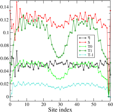
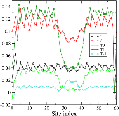
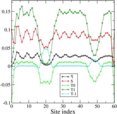
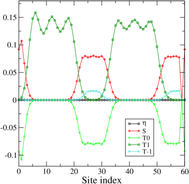
Figure 11: Various types of correlators $\langle A_{i}^{\dagger}A_{i+R}\rangle$ with the choices for $A_{i}$ written in (3) and the distance fixed to $R=1$. The model parameters here are $u=1$, $x=0.6$ and with OBC one can appreciate the spatial dependence on $i$. Upper panel: $m_{z}=0.1$ (left) and $m_{z}=0.15$ (right); lower panel: $m_{z}=0.25$ (left) and $m_{z}=0.40$ (right). Due to reflection symmetry only the left half of the chain is displayed.

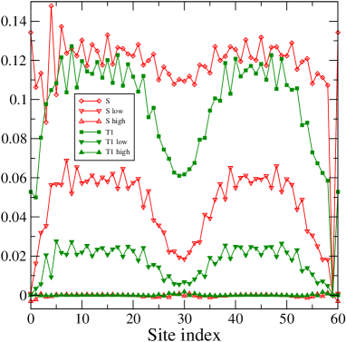
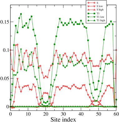
Figure 12: Same as figure 11 for the singlet and $T_{+1}$ correlation functions at distance $R=1$, where full up triangles now denote the “high” component and the empty down triangles denote the “low” one. Left panel is for $m_{z}=0.1$ while the right one is for $m_{z}=0.25$.

Qualitatively the result can be summarized as follows. On increasing the magnetization $m$ the spin-up electrons align along the field first in the high-density islands and then in the low-density ones. When in region (ii) the system exhibits FFLO oscillations in pair structure factor. When the domains finally appear at a macroscopic level ($m=m_{1}$), the FFLO pairs become mostly localized into the low density domains, and the corresponding peak is weakened; globally the system behaves as metal made of ferromagnetic domains alternating with superconducting ones. The SC properties of the low density domains fully disappear only when single electron localize ($m>m_{2}$), as shown by the right panel of figure 11.

6 Discussion and Conclusions

The results of the previous sections provide a coherent scenario of the physics of the SC phase described by the Hamiltonian (1) for $x\gtrsim 1/2$ in presence of non-vanishing magnetization. With respect to the case $x\leq 1/2$ (region (i)) , the different behaviour observed previously at $m=0$ persists up to high magnetization values ($m>m_{c}$), as a consequence of the rearrangement in the kinetic energies of holes and doublons which takes place at $x=0.5$ (see section II). The main features of the phase diagram in the $x-m$ plane are schematically shown in figure 13 for regions (ii) and (iii).

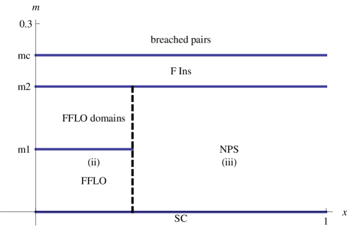
Figure 13: Schematic phase diagram at $0\leq u<u_{c}(x)$ and half-filling, in the $x-m$ plane for $x\geq 1/2$

At low magnetization the diagram shows evidence of the two regions, which turn out to behave differently up to $m=m_{2}$; here $m_{2}$ is the value at which the holes and minority spin single electrons localize into the low density domains, and the doublons localize into the high density domains: the system becomes insulating. In region (ii) SC persists in the whole system at non-zero magnetization up to $m=m_{1}<m_{2}$; the pair structure factor correspondingly shows a strong FFLO peak. Macroscopic phase separation appears on both the density and the magnetization profiles for $m>m_{1}$: in this case SC correlations become mainly confined to the low-density domains, whereas the system is still metallic due to the mobility of the single electrons. The low and high density regions display different magnetizations, so that for $m_{1}\leq m\leq m_{2}$ the system can be considered an itinerant ferromagnet, with superconducting FFLO domains. As for region (iii), there is no evidence for dominant SC correlations in the NPS phase as soon as $m\neq 0$; the system behaves as a liquid of $n_{s}$ single particles moving in a background of empty and doubly occupied sites textured into domains of microscopic size[16]. Macroscopic phase separation into high- and low-density domains appears on the density and magnetization profiles only for $m>m_{2}$, simultaneously with the transition to the insulating state. Finally, at a higher magnetization $m_{c}$, the regime of breached pairs described in [18] is entered.

We emphasize that the presence of a FFLO regime in the repulsive Hubbard model takes place for a range of values of the off-diagonal Coulomb repulsion ($1/2\lesssim x\lesssim 2/3$) in principle accessible to experiments. The results reported here for such regime are complementary to those obtained in [30] for the extended Hubbard model; in fact, they are expected to persist also in presence of non-vanishing nearest neighbor Coulomb repulsion, since similar incommensurate spin and charge correlations are observed also in that case [31]. The results are reminiscent for some aspects of those reported in [32] for the standard Hubbard model in the attractive $u$ region. We guess that our FFLO regime is to be identified to the weak LO (Larkin-Ovchinnikov) regime described there, whereas the regime of macroscopic phase separation of the high density polarized walls and the low density FFLO domains could well coincide with the strong LO regime discussed there, in which pair-pair correlations exhibit spatial dependence. The main difference we see with [32]is that in the present case with increasing the magnetization the domain walls (to be identified with our high density domains) tend to localize, in contrast to the delocalized behaviour observed there. Ultimately this feature is responsible for the transition to the insulating regime found here. We expect that the two scenarios could merge in the region of weakly attractive $u$ and $x\leq 0.5$.

As mentioned, with varying magnetization a second transition then occurs in both regions at $m=m_{2}$; in this case the system consists of two segregated metals of fully polarized single electrons with different Fermi momenta, which as a whole behave as a (ferrimagnetic) insulator. In two dimensions, we argue that the behaviour of such insulator could well be that of metallic stripes; whereas for $m_{1}\leq m\leq m_{2}$ in region (ii) the physics chould be that of a striped superconductor [33].

The analysis is performed here at finite size. Due to the different qualitative behaviour of the phases depicted in figure 13 the scenario should be considered quite plausible. A finite size scaling analysis is expected to provide a quantitative accurate derivation of the critical lines. In particular, since our study just considered two far apart typical points ($x=0.6$ for region (ii), and $x=0.8\mbox{ }$ for region (iii)), it is not possible to infer from it whether the change from region (ii) to (iii) is a smooth crossover or a true transition line.

References

References

- [1] Saxena S S et al., Superconductivity on the border of itinerant-electron ferromagnetism in UGe2, 2000 Nature 406 587
- [2] Marković N, Christiansen C and Goldman A M , Thickness-magnetic field phase diagram at the superconductor-insulator transition in 2D, 1998 Phys. Rev. Lett. 81 5217; Kim K and Stroud, Quantum Monte Carlo study of a magnetic-field-driven two-dimensional superconductor-insulator transition, 2008 Phys. Rev. B 78 174517
- [3] Kamihara Y, Watanabe T, Hirano M and Hosono H, Iron-based layered superconductor La[O1-xFx]FeAs () with =26K, 2008 J. Am. Chem. Soc. 130 3296
- [4] Park J T et al., Electronic phase separation in the slightly underdoped iron pnictide superconductor Ba1-xKxFe2As2, 2009 Phys. Rev. Lett. 102 117006
- [5] Lang G et al, Nanoscale electronic order in iron pnictides, 2010 Phys. Rev. Lett. 104 097001
- [6] Monthoux P, Pines D and Lonzarich G G, Superconductivity without phonons, 2007 Nature 450 1177
- [7] Fulde P, and Ferrell R A, Superconductivity in a strong spin-exchange field, 1964 Phys. Rev. 135 A550; Larkin A I and Ovchinnikov Yu N, Inhomogeneous state of superconductors, 1965 Sov. Phys. JETP 20 762
- [8] Koutroulakis G et al, Field evolution of coexisting superconducting and magnetic orders in CeCoIn5, 2010 Phys. Rev. Lett. 104 087001
- [9] Liao Y et al., Spin-imbalance in a one-dimensional Fermi gas, 2010 Nature 467 567
- [10] Eichenberger D and Baeriswyl D, Superconductivity and antiferromagnetism in the two-dimensional Hubbard model: A variational study, 2007 Phys. Rev. B 76 180504(R)
- [11] Hirsch J E, Bond-charge repulsion and hole superconductivity, 1989 Physica C 158 326; Hirsch J E and Marsiglio F, Superconducting state in an oxygen hole metal, 1989 Phys. Rev. B 39 11515
- [12] Gammel J T and Campbell D K, Comment on the missing bond-charge repulsion in the extended Hubbard model, 1988 Phys. Rev. Lett. 60 71
- [13] For reviews of recent results see [15, 22] below and also Nakamura M, Okano T and Itoh K, Exact bond-ordered ground states and excited states of the generalized Hubbard chain, 2005 Phys. Rev. B 72 115121; Dobry A O and Aligia A A, Quantum phase diagram of the half filled Hubbard model with bond-charge interaction, 2011 Nucl. Phys. B 843 767
- [14] Anfossi A, Degli Esposti Boschi C, Montorsi A and Ortolani F, Single-site entanglement at the superconductor-insulator transition in the Hirsch model, 2006 Phys. Rev. B 73 085113
- [15] Aligia A A, Anfossi A, Arrachea L, Degli Esposti Boschi C, Dobry A O, Gazza C, Montorsi A, Ortolani F and Torio M E, Incommmensurability and unconventional superconductor to insulator transition in the Hubbard Model with bond-charge interaction, 2007 Phys. Rev. Lett. 99 206401
- [16] Anfossi A, Degli Esposti Boschi C and Montorsi A, Nanoscale phase separation and superconductivity in the one-dimensional Hirsch model, 2009 Phys. Rev. B 79 235117
- [17] Montorsi A, Phase separation in fermionic systems with particle-hole asymmetry, 2008 J. Stat. Mech. L09001
- [18] Anfossi A, Barbiero L and Montorsi A, Phase diagram of imbalanced strongly interacting fermions on a one-dimensional optical lattice, 2009 Phys. Rev. A 80 043602
- [19] Roncaglia M, Degli Esposti Boschi C and Montorsi A, Hidden XY structure of the bond-charge Hubbard model, 2010 Phys. Rev. B 82 233105
- [20] For a review see Schollwöck U, The density-matrix renormalization group, 2005 Rev. Mod. Phys. 77 259
- [21] Giamarchi T, Quantum physics in one dimension, 2003 (Clarendon Press, Oxford)
- [22] Japaridze G I and Kampf A P, Weak-coupling phase diagram of the extended Hubbard model with correlated-hopping interaction, 1999 Phys. Rev. B 59 12822
- [23] Arrachea L and Aligia A A, Exact solution of a Hubbard chain with bond-charge interaction, 1994 Phys. Rev. Lett. 73 2240; de Boer J, Korepin V E and Schadschneider A, pairing as a mechanism of superconductivity in models of strongly correlated electrons, 1995 Phys. Rev. Lett. 74 789
- [24] Simon M E and Aligia A A, Brinkman-Rice transition in layered perovskites, 1993 Phys. Rev. B 48 7471
- [25] Dolcini F and Montorsi A, Finite-temperature properties of the Hubbard chain with bond-charge interaction, 2002 Phys. Rev. B 66 075112
- [26] Kemper A and Schadscneider A, Thermodynamic properties and thermal correlation lengths of a Hubbard model with bond-charge interaction, 2003 Phys. Rev. B 68 235102
- [27] Wang B and Duan L-M, Suppression or enhancement of the Fulde-Ferrell-Larkin-Ovchinnikov order in a one-dimensional optical lattice with particle-correlated tunneling, 2009 Phys. Rev. A 79 043612
- [28] Roscilde T et al., Quantum polarization spectroscopy of correlations in attractive fermionic gases, 2009 New J. Phys. 11 055041
- [29] Yamanaka M, Oshikawa M and Affleck I, Nonperturbative approach to Luttinger’s theorem in one dimension, 1997 Phys. Rev.Lett. 79 1110
- [30] Aizawa H, Kuroki K, Yokoyama T and Tanaka Y, Strong parity mixing in the Fulde-Ferrell-Larkin-Ovchinnikov superconductivity in systems with coexisting spin and charge fluctuations, 2009 Phys.Rev. Lett. 102 016403
- [31] Arrachea L, Gagliano E and Aligia A A, Ground-state phase diagram of an extended Hubbard chain with correlated hopping at half-filling, 1997 Phys. Rev. B 55 1173
- [32] Loh Y L and Trivedi N, Detecting the elusive Larkin-Ovchinnikov modulated superfluid phases for imbalanced Fermi gases in optical lattices, 2010 Phys. Rev. Lett. 104 165302
- [33] Berg E, Fradkin E, Kivelson S A and Tranquada J M, Striped superconductors: how spin, charge and superconducting orders intertwine in the cuprates, 2009 New J. Phys 11 115004