Multimer formation in 1D two-component gases and trimer phase in the asymmetric attractive Hubbard model

Abstract

We consider two-component one-dimensional quantum gases at special imbalanced commensurabilities which lead to the formation of multimer (multi-particle bound-states) as the dominant order parameter. Luttinger liquid theory supports a mode-locking mechanism in which mass (or velocity) asymmetry is identified as the key ingredient to stabilize such states. While the scenario is valid both in the continuum and on a lattice, the effects of umklapp terms relevant for densities commensurate with the lattice spacing are also mentioned. These ideas are illustrated and confronted with the physics of the asymmetric (mass-imbalanced) fermionic Hubbard model with attractive interactions and densities such that a trimer phase can be stabilized. Phase diagrams are computed using density-matrix renormalization group techniques, showing the important role of the total density in achieving the novel phase. The effective physics of the trimer gas is as well studied. Lastly, the effect of a parabolic confinement and the emergence of a crystal phase of trimers are briefly addressed. This model has connections with the physics of imbalanced two-component fermionic gases and Bose-Fermi mixtures as the latter gives a good phenomenological description of the numerics in the strong-coupling regime.

I Introduction

The notions of quantum liquids and their instabilities are paradigmatic for condensed matter physics Leggett2006 . For multicomponent fluids, an important set of instabilities is associated with interactions between components. A classic example is the Cooper instability of a spin-$1/2$ Fermi liquid : even an infinitesimal attractive coupling between fermions of opposite spins drives a phase transition into the Bardeen-Cooper-Schrieffer superconductor Schrieffer1999 . A one-dimensional (1D) counterpart of the Fermi liquid, the spinful Luttinger liquid, has a similar instability, where an attractive inter-spin coupling opens a gap in the spin channel Giamarchi1995 ; Giamarchi2004 .

Traditionally, the bulk of the discussion on two-species liquids assumed the SU(2) spin symmetry. The recent years have witnessed a growing availability of experimental studies of mixtures of unlike particles. This includes loading ultracold atoms to spin-dependent optical lattices Mandel2003 , and trapping atoms of different masses Wille2008 or even different statistics Giorgini2008 . While most of experimental progress so far is in the domain of ultracold atoms, we stress that the relevance of such asymmetric mixtures is not confined to the realm of cold gases : dealing with more traditional solid state systems, one faces an asymmetric mixture situation as soon as the Fermi level spans several bands (which a priori need not be equivalent). This setup is typical for such diverse materials as semi-metallic compounds, mixed-valence materials, organic superconductors Penc1990 , small radius nanotubes Carpentier2006 , and even graphene-based heterostructures Martin2008 .

A generic question immediately arises : given a two-component mixture, what is the role of (the lack of) SU(2) symmetry? Or, more precisely, does the symmetry between components limit the set of instabilities of a liquid? Clearly, the answer might depend on the universality class of the liquid, and on the particular way the symmetry is broken. The simplest albeit non-trivial way of breaking the symmetry is to assume species-dependent masses of the particles. Even if we consider the few-body problem, this is known to bring new physics like the Efimov phenomenon : while for an equal-mass Fermi liquid the only allowed bound state is a Cooper pair, three-body bound states (trimers) appear once the mass ratio exceeds a certain threshold Braaten2006 . The atom-dimer scattering is strongly affected by the mass asymmetry  Petrov2003 and the ultimate fate of a Fermi liquid in presence of the Efimov effect is currently an open question being actively investigated Levinsen2009 . All these theoretical considerations are strongly motivated by cold-atom experiments which have recently achieved degeneracy of Fermi gases with different masses Wille2008 and spin-imbalanced two-component fermionic gases Partridge2006 .

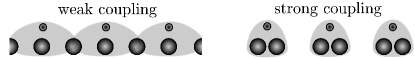
Figure 1: Qualitative formation of trimers in the weak-coupling picture of the bosonization (on the left) and in the strong-coupling picture for large interactions (on the right).

The physics of 1D quantum many-body systems offers powerful methods Giamarchi2004 , both analytical and numerical, to have quantitative predictions on the fate of the Luttinger liquid in the presence of perturbations. The role of mass asymmetry for a two-component Luttinger liquid has been investigated in the renormalization group (RG) framework originally in the context of solid state physics Muttalib1986 ; Penc1990 ; Loss1994 , and recently revisited mostly in the context of cold atoms Cazalilla2003 ; Mathey2004 ; Cazalilla2005 ; Mathey2007 ; Mathey2007a ; Lu2009 ; Crepin2010 ; Orignac2010 ; Tsvelik2010 , and supplemented by numerical investigations Pollet2006 ; Mering2008 ; Batrouni2009 ; Wang2009 . Overall the consensus was that the only new instability arising due to asymmetry is the collapse (demixing) instability for large asymmetry and/or strong interspecies attraction (repulsion). Recently, a novel family of instabilities was predicted Burovski2009 to exist due to the interplay between polarization and asymmetry : These instabilities only take place for polarized mixtures of either statistics, and are characterized by the locking of the ratio of the densities to a rational value. Subsequent work in Ref. Orso2010, elucidated the relation of these instabilities and existence of few-body bound states. A qualitative picture of the mode-locking mechanism and the strong-coupling limit of the trimer formation is given in Fig. 1. The latter regime recalls another approach to multi-particle bound-states which is the use of many-colors ($N$-component) fermions Wu2005 ; Capponi2008 ; Roux2009 with which the physics of the trimers share qualitative features.

This paper is divided in two main parts : the first one investigates in detail the bosonization approach and the mode-locking mechanism mentioned above, while the second is dedicated to the specific but important example of the 1D asymmetric Hubbard model using the density-matrix renormalization group (DMRG) technique White1992 . The predictions of the first part account for most of the numerical data, but a more phenomenological Bose-Fermi picture is proposed as a complementary analysis. Other important questions such as the effect of a trapping potential or the emergence of crystal phases are eventually addressed.

II Bosonization analysis

In this section, we describe the salient features of the effective bosonic field theory appropriate to a 1D mixture of two distinct fermionic (or bosonic) atoms. The aim of this section is to give a bosonization interpretation for the formation of few-body bound states and their effective behavior through a mode-locking mechanism between the two species. Predictions on the nature of the resulting phase are then made. The theory is a priori valid for models in the continuum or the continuous version of lattice models at generic (i.e. non-commensurate) densities. The effects of the presence of the lattice on certain commensurate densities will be briefly discussed in section II.4. Notation conventions are standard and taken from Ref. Giamarchi2004, .

II.1 Mode locking mechanism

The two species are labeled by a pseudo-spin index $\sigma={\uparrow,\downarrow}$ and their corresponding densities $n_{\sigma}$ such that $n=n_{\uparrow}+n_{\downarrow}$ is the total density. Each species can be described by a scalar field $\phi_{\sigma}$ and its dual $\theta_{\sigma}$. The creation operators can be expressed as a function of these fields, with, for fermions

$$\Psi^{\dagger}_{\sigma}(x)\sim\Big{(}n_{\sigma}-\frac{1}{\pi}\partial_{x}\phi_{\sigma}\Big{)}^{1/2}\sum_{p}e^{i(2p+1)(k_{\sigma}x-\phi_{\sigma})}\,e^{-i\theta_{\sigma}}\,,$$ (1)

and, for bosons,

$$b^{\dagger}_{\sigma}(x)\sim\Big{(}n_{\sigma}-\frac{1}{\pi}\partial_{x}\phi_{\sigma}\Big{)}^{1/2}\sum_{p}e^{i2p(k_{\sigma}x-\phi_{\sigma})}\,e^{-i\theta_{\sigma}}\;.$$ (2)

We have included all higher harmonics : as a consequence, the summation is over all integers Haldane1981 . The “Fermi momenta”, $k_{\sigma}=\pi n_{\sigma}$ are a priori not equal to each other, corresponding to a spin-imbalanced situation. The density operators $\hat{n}_{\sigma}$ read

$$\hat{n}_{\sigma}(x)\sim\Big{(}n_{\sigma}-\frac{1}{\pi}\partial_{x}\phi_{\sigma}\Big{)}\sum_{p}e^{i2p(k_{\sigma}x-\phi_{\sigma})}\;.$$ (3)

The effective low-energy Hamiltonian can be written in terms of the fields $\phi_{\sigma}$ and their canonically conjugate momentum $\Pi_{\sigma}=\partial_{x}\theta_{\sigma}/\pi$. In the case of absence of inter-species interactions the effective bosonic theory is given by $\mathcal{H}_{0}(\phi_{\uparrow})+\mathcal{H}_{0}(\phi_{\downarrow})$, where

$$\mathcal{H}_{0}(\phi_{\sigma})=\dfrac{v_{\sigma}}{2\pi}\int\!dx\,\left[K_{\sigma}(\pi\Pi_{\sigma})^{2}+K_{\sigma}^{-1}\left(\partial_{x}\phi_{\sigma}\right)^{2}\right]\;,$$ (4)

where $v_{\sigma}$ is the sound velocity and $K_{\sigma}$ the so-called Luttinger parameter, which is equal to one in the free fermions or free hard-core bosons cases. Taking into account density-density interactions between species, of the generic form $\int\!dxdx^{\prime}\,U(x-x^{\prime})\hat{n}_{\uparrow}(x)\hat{n}_{\downarrow}(x^{\prime})$, changes the effective theory and brings new kinds of terms : zero-momentum terms in the density representation (3) couples the two spin species through a bilinear operator

$$\mathcal{H}_{1}=\frac{g}{2\pi}\int\!dx\,(\partial_{x}\phi_{\uparrow})(\partial_{x}\phi_{\downarrow})\;,$$ (5)

where $g$ is a forward scattering constant, and higher harmonics terms involving multiples of the spatial frequencies $k_{\sigma}$ :

$$\sum_{p,q>0}G_{pq}^{\pm}\!\int\!dx\,\cos{\big{[}2\pi(pn_{\uparrow}\pm qn_{\downarrow})x-2(p\phi_{\uparrow}\pm q\phi_{\downarrow})\big{]}}$$ (6)

where $G_{pq}^{\pm}$ are non-universal coupling constants. Clearly, if the generalized commensurability condition

$$p\,n_{\uparrow}-qn_{\downarrow}=0\;,$$ (7)

is satisfied (with $p$ and $q$ coprime integers), and provided these terms are relevant, they will tend to lock the up and down fields together. When the densities are fine-tuned to the definite commensurability (7), then all other cosine operators in the sum are oscillating, in which case they don’t contribute in the continuum limit (or they are less relevant for multiples of $p$ and $q$). The remaining important operator in the sum (6) is thus the sine-Gordon term

$$\mathcal{H}_{2}=G\int\!dx\,\cos{\sqrt{8}\phi_{a}}\;,$$ (8)

with the combination

$$\phi_{a}=\frac{1}{\sqrt{2}}(p\phi_{\uparrow}-q\phi_{\downarrow})\;.$$ (9)

For attractive interactions $G<0$ (we will argue below that this choice favors the relevance of the term), energy will be minimized when the field is pinned to $\langle{\phi_{a}}\rangle=0$. Notice again that the above argument on the mode-locking mechanism does not rely on the presence of a lattice. Lastly, the cosine locks a combination of the bosonic modes but at a generic total density $n$, there remains another bosonic mode leaving the full excitation spectrum gapless. We will see that the latter describes the effective behavior of the bound-states. In the following, we dub $\phi_{b}$ this massless bosonic mode.

We can draw a last remark on the operators (6) : they have high scaling dimensions near the free fermion fixed point and are expected to be irrelevant apart from some special circumstances which are the object of this work. In the fermionic language, they involve $(p+q)$-body interactions of the form:

$$\sum_{\{k\}}\prod_{i=1}^{q}\psi^{\dagger}_{R\downarrow}(k_{i})\psi_{L\downarrow}(k_{i}^{\prime})\,\prod_{j=1}^{p}\psi^{\dagger}_{L\uparrow}(k_{j}^{\prime\prime})\psi_{R\uparrow}(k_{j}^{\prime\prime\prime})+\mathrm{h.c.}\;,$$ (10)

where the summation over $\{k\}$ runs over all combinations of $2(p+q)-1$ momenta due to the total momentum conservation law : $\sum_{i=1}^{q}(k_{i}-k_{i}^{\prime})+\sum_{j=1}^{p}(k_{j}^{\prime\prime}-k_{j}^{\prime\prime\prime})=0$. Such interactions appear at high order in perturbation theory in a Hubbard model for example or after several steps of a RG treatment. For practical purposes it is simpler to work with the bosonic formulation given by Eq. (8), and this is what we do from now on.

In the following, we assume that the densities are commensurate via the condition (7), and analyze the simplified effective theory written in terms of the $\uparrow$ and $\downarrow$ fields

$$\mathcal{H}=\mathcal{H}_{0}(\phi_{\uparrow})+\mathcal{H}_{0}(\phi_{\downarrow})+\mathcal{H}_{1}+\mathcal{H}_{2}\;,$$ (11)

where the velocities $v_{\sigma}$ and Luttinger parameters $K_{\sigma}$ are determined by the intra-species interactions. The quadratic part $\mathcal{H}_{0}(\phi_{\uparrow})+\mathcal{H}_{0}(\phi_{\downarrow})+\mathcal{H}_{1}$ can be diagonalized by a Bogoliubov transformation Engelsberg1964 which could give a starting point for a perturbative RG calculation Penc1990 ; Cazalilla2003 ; Cazalilla2005 ; Mathey2007 ; Crepin2010 . Due to the velocity asymmetry, additional couplings are generated and velocities are renormalized along the flow. The discussion of the nature of the gapped phases and their correlations remains unclear. In particular, diagonalizing the quadratic part $\mathcal{H}_{0}(\phi_{\uparrow})+\mathcal{H}_{0}(\phi_{\downarrow})+\mathcal{H}_{1}$ of the Hamiltonian (11) does not give, apart from special choice of the parameters, the combination (9) that appears in the cosine term $\mathcal{H}_{2}$. In the next section, we take the following strategy : we look for the conditions under which the quadratic part and the cosine term are simultaneously diagonalizable. At the price of a restriction on the parameters range, the analysis can be done safely both for the criteria of relevance of the cosine and for the correlation functions in the single-mode phase. In spite of the limitation of the approach, we believe the scenario does occur without this restriction : as shown numerically in Sec. III on a realistic model, the single-mode multimer phase can span a wide region of the phase diagram.

Lastly, we notice that, similarly to the phase separation criteria in two-component mixtures (when one of the mode velocities vanishes), the single-mode phase will undergo a phase separation instability when the gapless mode velocity $v_{b}$ vanishes. We thus expect to find the single-mode phase surrounded with the two-mode phase and a demixed phase.

II.2 Field transformation

We have qualitatively discussed the fact that the physics should generically be described by two fields $\phi_{s}$ where $s=a,b$, with $\phi_{a}=(p\phi_{\uparrow}-q\phi_{\downarrow})/\sqrt{2}$ being the one entering in the cosine term (8). In general, it is hard to have a complete form for the transformation between the $\phi_{s}$ and the $\phi_{\sigma}$. Such a transformation is important both for the RG analysis and the calculation of physical correlators which are naturally expressed in terms of the $\phi_{\sigma},\theta_{\sigma}$ fields. Below, we discuss a special case where the transformation can be performed and its range of validity.

The simplest transformation, and yet rather general, one can work with is a linear combination of the fields with coefficients that are independent of the position :

$$\phi_{\uparrow} =\mathfrak{p}_{a\uparrow}\phi_{a}+\mathfrak{p}_{b\uparrow}\phi_{b}\,, \theta_{\uparrow} =\mathfrak{t}_{a\uparrow}\theta_{a}+\mathfrak{t}_{b\uparrow}\theta_{b}\,,$$ (12)

$$\phi_{\downarrow} =\mathfrak{p}_{a\downarrow}\phi_{a}+\mathfrak{p}_{b\downarrow}\phi_{b}\,, \theta_{\downarrow} =\mathfrak{t}_{a\downarrow}\theta_{a}+\mathfrak{t}_{b\downarrow}\theta_{b}\,.$$ (13)

When $p\neq q$, excitations corresponding to the eigenmodes $\phi_{a,b}$ carry both spin and charge modes which are respectively the sum and the difference of the $\uparrow$ and $\downarrow$ modes. As the transformation must preserve the commutation relations

$$[\theta_{\sigma}(x),\nabla\phi_{\sigma^{\prime}}(x^{\prime})] =i\pi\delta_{\sigma\sigma^{\prime}}\delta(x-x^{\prime})\,,$$ (14)

$$[\phi_{\sigma}(x),\nabla\theta_{\sigma^{\prime}}(x^{\prime})] =i\pi\delta_{\sigma\sigma^{\prime}}\delta(x-x^{\prime})\,,$$ (15)

we get that $\mathfrak{p}_{a\sigma}\mathfrak{t}_{a\sigma^{\prime}}+\mathfrak{p}_{b\sigma}\mathfrak{t}_{b\sigma^{\prime}}=\delta_{\sigma\sigma^{\prime}}$. Then, we have

$$\mathfrak{t}_{a\uparrow} =\mathfrak{p}_{b\downarrow}/D\,, \mathfrak{t}_{a\downarrow} =-\mathfrak{p}_{b\uparrow}/D\,,$$ (16)

$$\mathfrak{t}_{b\uparrow} =-\mathfrak{p}_{a\downarrow}/D\,, \mathfrak{t}_{b\downarrow} =\mathfrak{p}_{a\uparrow}/D\,,$$ (17)

with the determinant

$$D=\mathfrak{p}_{a\uparrow}\mathfrak{p}_{b\downarrow}-\mathfrak{p}_{a\downarrow}\mathfrak{p}_{b\uparrow}=(\mathfrak{t}_{a\uparrow}\mathfrak{t}_{b\downarrow}-\mathfrak{t}_{a\downarrow}\mathfrak{t}_{b\uparrow})^{-1}\,.$$ (18)

In a shortened version, we have $\phi_{\sigma}=\mathcal{P}\phi_{s}$, where $\mathcal{P}$ is the matrix of the $\mathfrak{p}$, and $\theta_{\sigma}=(\mathcal{P}^{-1})^{t}\theta_{s}$. If $\mathcal{P}$ is unitary, the $\theta$ and the $\phi$ undergo the same transformation.

We now impose that $\phi_{a}=(p\phi_{\uparrow}-q\phi_{\downarrow})/\sqrt{2}$ which gives

$$\mathfrak{t}_{a\uparrow} =\frac{p}{\sqrt{2}}\;, \mathfrak{t}_{a\downarrow} =-\frac{q}{\sqrt{2}}\,.$$ (19)

As we want to cancel the cross-terms in Eq. (11), we require that :

$$v_{\uparrow}K_{\uparrow}\mathfrak{t}_{a\uparrow}\mathfrak{t}_{b\uparrow} =-v_{\downarrow}K_{\downarrow}\mathfrak{t}_{a\downarrow}\mathfrak{t}_{b\downarrow}\,,$$ (20)

$$\frac{v_{\uparrow}}{K_{\uparrow}}\mathfrak{p}_{a\uparrow}\mathfrak{p}_{b\uparrow}+\frac{v_{\downarrow}}{K_{\downarrow}}\mathfrak{p}_{a\downarrow}\mathfrak{p}_{b\downarrow} =-g(\mathfrak{p}_{a\downarrow}\mathfrak{p}_{b\uparrow}+\mathfrak{p}_{a\uparrow}\mathfrak{p}_{b\downarrow})\,,$$ (21)

which can be rewritten as :

$$pv_{\uparrow}K_{\uparrow}\mathfrak{t}_{b\uparrow}\quad- qv_{\downarrow}K_{\downarrow} \mathfrak{t}_{b\downarrow}=0$$ (22)

$$-\Big{(}p\frac{v_{\downarrow}}{K_{\downarrow}}+gq\Big{)}\mathfrak{t}_{b\uparrow}\quad+ \displaystyle\Big{(}q\frac{v_{\uparrow}}{K_{\uparrow}}+gp\Big{)} \mathfrak{t}_{b\downarrow}=0\;.$$ (23)

There exists a non-zero solution only if the condition :

$$v_{\uparrow}\Big{(}v_{\uparrow}+\frac{gp}{q}K_{\uparrow}\Big{)}=v_{\downarrow}\Big{(}v_{\downarrow}+\frac{gq}{p}K_{\downarrow}\Big{)}$$ (24)

is satisfied. When this condition is satisfied, we have a one-parameter family of transformations with the desirable property of having only one eigenmode in the argument of the cosine operator. The parameter is just the choice of scale of the field $\phi_{b}$ : in 1D, we can change the scale of the Bose field provided we change accordingly its Luttinger parameter $K_{b}$. Here, we choose the scale of $\phi_{b}$ so that :

$$\mathfrak{t}_{b\uparrow} =\frac{q}{\sqrt{2}}\sqrt{\frac{v_{\downarrow}}{v_{\uparrow}}}K_{\downarrow}\;, \mathfrak{t}_{b\downarrow} =\frac{p}{\sqrt{2}}\sqrt{\frac{v_{\uparrow}}{v_{\downarrow}}}K_{\uparrow}\,,$$ (25)

The condition (24) strongly reduces the range of applicability of the transformation : for a given coupling $g$, the Luttinger parameters and velocities of each species must satisfy the above relation. When the transformation can be used, (11) splits into a free boson field for $b$ and a sine-Gordon model for $a$ : $\mathcal{H}=\mathcal{H}_{0}(\phi_{b})+\mathcal{H}_{\text{sG}}(\phi_{a})$ with $\mathcal{H}_{\text{sG}}=\mathcal{H}_{0}+\mathcal{H}_{2}$. In this case, the new velocities and Luttinger parameters associated with the $a,b$ modes are given by the following relations :

$$v_{a}^{2} =\frac{\sqrt{v_{\uparrow}v_{\downarrow}}}{2\mathcal{K}}\Big{(}p^{2}v_{\uparrow}K_{\uparrow}\frac{v_{\uparrow}}{v_{\downarrow}}+q^{2}v_{\downarrow}K_{\downarrow}\frac{v_{\downarrow}}{v_{\uparrow}}-gpqK_{\uparrow}K_{\downarrow}\Big{)}\,,$$

$$K_{a} =\mathcal{K}\frac{\sqrt{v_{\uparrow}v_{\downarrow}}}{v_{a}}\,,$$ (26)

$$v_{b}^{2} =\frac{\sqrt{v_{\uparrow}v_{\downarrow}}}{2\mathcal{K}}\left(p^{2}v_{\downarrow}K_{\uparrow}+q^{2}v_{\uparrow}K_{\downarrow}+gpqK_{\uparrow}K_{\downarrow}\right)\,,$$

$$K_{b} =K_{\uparrow}K_{\downarrow}\mathcal{K}\frac{\sqrt{v_{\uparrow}v_{\downarrow}}}{v_{b}}\,.$$

where we have defined :

$$\mathcal{K}=\frac{p^{2}v_{\uparrow}K_{\uparrow}+q^{2}v_{\downarrow}K_{\downarrow}}{2\sqrt{v_{\uparrow}v_{\downarrow}}}\,.$$ (27)

With our definition of $\phi_{a}$ and provided the sine-Gordon description is applicable, the requirement for the cosine to be relevant, and thus to enter the single-mode phase, is simply

$$K_{a}<1\;.$$ (28)

One qualitatively observes that a velocity much smaller than the other favors a small $K_{a}$ and that large attractive interactions $g<0$ will help increase $v_{a}$ and reduce $K_{a}$. In the following, we consider limiting cases in which the discussion simplifies in order to identify how the parameters would favor the formation of a gap in the $a$ sector.

The limit $v_{b}^{2}=0$ (attained with attractive interactions) signals the transition to the phase-separated or Falicov-Kimball regime from the multimer phase.

II.2.1 The case of equal velocities

When $v_{\uparrow}=v_{\downarrow}=v_{0}$, the condition (24) imposes that either (i) $g=0$ or (ii) $\displaystyle\frac{K_{\uparrow}}{K_{\downarrow}}=\frac{q^{2}}{p^{2}}$. The transformation and new velocities and Luttinger parameters then take a simple form : in case (i), we have $v_{a}=v_{b}=v_{0}$ and :

$$\phi_{a} =\frac{1}{\sqrt{2}}(p\phi_{\uparrow}-q\phi_{\downarrow})\,, \phi_{b} =\frac{1}{\sqrt{2}}\left(qK_{\downarrow}\phi_{\uparrow}+pK_{\uparrow}\phi_{\downarrow}\right)\,,$$

$$K_{a} =\frac{p^{2}K_{\uparrow}+q^{2}K_{\downarrow}}{2}\,, K_{b} =K_{\uparrow}K_{\downarrow}\frac{p^{2}K_{\uparrow}+q^{2}K_{\downarrow}}{2}\,.$$ (29)

while in case (ii), we have $\mathcal{K}=p^{2}K_{\uparrow}$ and

$$\phi_{a} =\frac{1}{\sqrt{2}}(p\phi_{\uparrow}-q\phi_{\downarrow})\,, \phi_{b} =\frac{pK_{\uparrow}}{q\sqrt{2}}\left(p\phi_{\uparrow}+q\phi_{\downarrow}\right)\,,$$

$$v_{a}^{2} =v_{0}^{2}\Big{(}1-\frac{gp}{2qv_{0}}K_{\uparrow}\Big{)}\,, v_{b}^{2} =v_{0}^{2}\Big{(}1+\frac{gp}{2qv_{0}}K_{\uparrow}\Big{)}\,,$$

$$K_{a} =p^{2}K_{\uparrow} K_{b} =\frac{p^{4}K_{\uparrow}^{3}}{q^{2}\sqrt{1+\frac{gp}{2qv_{0}}K_{\uparrow}}}\,.$$

In both cases, having $K_{a}<1$ would require a very small $K_{\uparrow}$ (assuming $q=1$ for example). This could be realized with long-range intra-species interactions but may not be easily achievable. Notice a peculiarity of the formula for the massive mode $\phi_{b}$ in (29): while $K_{\uparrow}$ and $K_{\downarrow}$ are length-scale dependent (in the RG sense), the expression in (29) holds on all length-scales.

II.2.2 The limit of large asymmetry

In order to identify the influence of the velocities ratio on $K_{a}$, one can introduce the dimensionless quantities $\nu=v_{\downarrow}/v_{\uparrow}$, $\rho=q/p$ and $\gamma=g/v_{\uparrow}$. Then, (24) and (26) are rewritten as

$$1+\rho\gamma K_{\uparrow} =\nu(\nu+\gamma\rho^{-1}K_{\downarrow})\,,$$ (30)

$$K_{a} =\nu\frac{K_{\uparrow}+\rho\nu K_{\downarrow}}{K_{\uparrow}-\rho\gamma K_{\uparrow}K_{\downarrow}\nu+\rho^{2}K_{\downarrow}\nu^{3}}\,.$$ (31)

If one takes into account (31) only, $K_{a}$ vanishes in the limit of large velocity ratio $\nu\rightarrow 0$ or $\infty$ and passes through a maximum in between so that there are two windows of $\nu$ such that $K_{a}<1$. The smaller the maximum, the wider these windows are so, clearly, negative and large interactions ($\gamma<0$) favor the mode-locking mechanism. Yet, (30) imposes another constraint and we just consider the $\nu\rightarrow 0$ limit for simplicity. There, this limit is possible provided $K_{\uparrow}\simeq-1/\gamma\rho$, i.e. in the case of attractive interaction only. As a consequence, this analysis shows that we should expect the formation of multimer in the attractive and large interaction regime, favored by large asymmetry.

II.2.3 In the single-mode Luttinger liquid phase

Deep in the massive-$a$ phase, one can make a crude quadratic approximation to the cosine operator in (8) by replacing it with a mass term $\propto(p\phi_{\uparrow}-q\phi_{\downarrow})^{2}$. This leads to approximate expressions for the velocity and Luttinger parameter of the remaining mode $b$ :

$$v_{b}^{2} =v_{\uparrow}v_{\downarrow}\frac{p^{2}K_{\uparrow}v_{\downarrow}+q^{2}K_{\downarrow}v_{\uparrow}}{p^{2}K_{\uparrow}v_{\uparrow}+q^{2}K_{\downarrow}v_{\downarrow}}\;,$$

$$K_{b} =\frac{1}{2}K_{\uparrow}K_{\downarrow}\frac{(p^{2}K_{\uparrow}+q^{2}K_{\downarrow})^{2}}{\sqrt{p^{2}\frac{K_{\uparrow}}{v_{\uparrow}}+q^{2}\frac{K_{\downarrow}}{v_{\downarrow}}}\sqrt{p^{2}{K_{\uparrow}}{v_{\downarrow}}+q^{2}{K_{\downarrow}}{v_{\uparrow}}}}\;,$$

which reduces to the correct result for equal velocities.

II.3 Correlation functions and the nature of the phases

In one-dimensional models, the classification of the groundstates is determined by their dominant correlations. One can break discrete symmetries (for instance translational symmetry on a lattice model) but order parameters associated with continuous symmetries are always zero. The naming of a phase then corresponds to the connected equal-time correlator with the slowest decay in space. Quite generally, these correlators are asymptotically decaying either algebraically or exponentially. Such algebraic correlations are usually referred to as a quasi long-range order (QLRO). The slowest decay (or smallest exponent of algebraic correlations) criteria is based on a RPA argument by considering a set of weakly coupled Luttinger liquids Giamarchi2004 which shows that order will build up provided the exponent of the correlator is smaller than two, and that the main instability is associated with the smallest exponent. However, if the Green’s function, associated with $\Psi_{\sigma}$ which is not an order parameter, has the slowest decaying exponent, a RG analysis shows that coupling the Luttinger liquids yield a Fermi liquid phase (provided that the decay exponent is smaller than two again). If all physical correlators are exponentially decaying (apart from the density one which always keep, at least, a quadratic decay), the term liquid is often used. This approach yet remains phenomenological as the higher-dimension situation and is much more involved.

In this section, we follow the standard practice and consider the correlation functions of various observables to discuss the nature of the phases that are realized in the single-mode and two-mode regimes. The asymptotic decay of the connected correlation functions associated with the order parameter $\mathcal{O}(x)$ typically reads $\langle\mathcal{O}(0)\mathcal{O}^{\dagger}(x)\rangle_{c}\propto x^{-\alpha_{\mathcal{O}}}$ with some exponent $\alpha_{\mathcal{O}}$. In order to compute the correlators, we only keep the first harmonics in Eq. (1) and begin with the richer case of fermions where we use the representation in terms of right and left movers:

$$\Psi_{\sigma}(x)\sim e^{ik_{\sigma}x}e^{i(\theta_{\sigma}-\phi_{\sigma})}+e^{-ik_{\sigma}x}e^{i(\theta_{\sigma}+\phi_{\sigma})}\,.$$ (32)

We use the results that when a field $\phi_{a}$ is pinned, $\langle{f(\phi_{a})}\rangle=f(\langle{\phi_{a}}\rangle)$ and its dual $\theta_{a}$ is disordered, leading to an exponential decay. In the case of algebraic correlations, the decay exponents are obtained using the result that, for a field $\phi$ described by $\mathcal{H}_{0}$, the equal-time correlator associated with $\displaystyle A_{m,n}(x)=e^{i[m\phi(x)+n\theta(x)]}$ behaves asymptotically as

$$\langle{A_{m,n}(x)A_{-m,-n}(0)}\rangle\propto x^{-(m^{2}K+n^{2}/K)/2}\;.$$ (33)

We now give the leading contributions of the order parameters as a function of the $a,b$ fields, assuming general transformation coefficients of the $\uparrow$ and $\downarrow$ modes :

$$\Psi_{\sigma}(x) \sim e^{ik_{\sigma}x}e^{-i[\mathfrak{p}_{a\sigma}\phi_{a}+\mathfrak{p}_{b\sigma}\phi_{b}-\mathfrak{t}_{a\sigma}\theta_{a}-\mathfrak{t}_{b\sigma}\theta_{b}]}$$ Green’s function (34)

$$\hat{n}_{\sigma}(x) \sim-\mathfrak{p}_{a\sigma}\nabla\phi_{a}-\mathfrak{p}_{b\sigma}\nabla\phi_{b}+\Lambda^{-1}\cos(2k_{\sigma}x-2(\mathfrak{p}_{a\sigma}\phi_{a}+\mathfrak{p}_{b\sigma}\phi_{b}))$$ density (35)

$$\Psi_{\uparrow}(x)\Psi_{\downarrow}(x) \sim e^{i(k_{\uparrow}-k_{\downarrow})x}e^{-i[(\mathfrak{p}_{a\downarrow}-\mathfrak{p}_{a\uparrow})\phi_{a}+(\mathfrak{p}_{b\downarrow}-\mathfrak{p}_{b\uparrow})\phi_{b}+(\mathfrak{t}_{a\downarrow}+\mathfrak{t}_{a\uparrow})\theta_{a}+(\mathfrak{t}_{b\downarrow}+\mathfrak{t}_{b\uparrow})\theta_{b}]}$$ singlet pairing (36)

$$\Psi_{\sigma}(x)\Psi_{\sigma}(x) \sim e^{2i[\mathfrak{t}_{a\sigma}\theta_{a}+\mathfrak{t}_{b\sigma}\theta_{b}]}$$ triplet pairing (37)

where $\Lambda$ is a short-range cutoff. Among the multiple combinations of right and left movers, we have chosen the ones which should lead to the lowest decay exponents, by having the lowest $m$ and $n$ constant. They usually correspond to the smallest wave-vector.

II.3.1 The two-mode Luttinger liquid (2M-LL) phase

In the two mode-regime, all correlators are algebraic and the leading one will strongly depend on the actual coefficients of the transformation. The expression of Eqs. (34)–(37) are here understood with general transformation coefficients of the $\uparrow$ and $\downarrow$ modes as one does not necessarily have to impose the restriction (19) since $\phi_{a}$ does not here identify with (9). The transformation coefficients can be computed exactly Mathey2004 ; Mathey2007a in the absence of the cosine term (8). The correlation functions can as well be computed directly using a Green’s function approach Orignac2010 . In the presence of (8), the coefficients will be renormalized in this two-mode phase to unknown values. This regime is rather generic and, depending on the interaction and densities, with many competing orders among which are a Fermi liquid-like phase, a superconducting singlet or triplet FFLO phase Fulde1964 (pairing correlations displaying the typical $k_{\downarrow}-k_{\uparrow}$), a spin-density wave (SDW) or charge-density wave (CDW) phase. The case of equal densities, $p=q=1$ has the dominant channels Giamarchi2004 among the superconducting, CDW, and SDW fluctuations. In the cases where spin and charge degrees of freedom separate, CDW and SDW states are mutually exclusive. Furthermore, for SU(2)-symmetric models, $x$-, $y$- and $z$-components of the SDW order parameter are degenerate. These last remarks are no longer valid in our situation.

II.3.2 The single-mode Luttinger (1M-LL) multimer phase

Another regime corresponds to the case where the cosine in Eq. (8) is relevant in the RG sense. Then, the system has a massive mode $\phi_{a}$ given by (9), and a massless mode $\phi_{b}$. The massless mode is described in the low-energy limit by a free bosonic with a velocity $v_{b}$ and a Luttinger parameter $K_{b}$. In this single-mode Luttinger liquid, algebraic decays will be ruled by this $K_{b}$ Luttinger parameter when they occur. When the parameters of the problem satisfy Eq. (24), then the massless mode can be found explicitly. In this section we use these results to discuss in details the behavior of the correlation functions.

When $\phi_{a}$ gets pinned, we see that the above correlators (34)–(37) are all exponential because the presence of $\theta_{a}$ in their expression, with the exception of the density one. In particular, all two-body pairing channels are suppressed, even in the presence of attractive interactions. In order to construct an operator which has algebraic correlations, the prefactor in front of $\theta_{a}$ must vanish. This is realized by taking the $(p+q)$-mer combination $\Psi_{\uparrow}^{q}(x)\Psi_{\downarrow}^{p}(x)$ (bound states of $p$ $\downarrow$-fermions with $q$ $\uparrow$-fermions) which has the prefactor $q\mathfrak{t}_{a\uparrow}+p\mathfrak{t}_{a\downarrow}$ which is clearly zero from (19):

$$\Psi_{\uparrow}^{q}(x)\Psi_{\downarrow}^{p}(x) \sim e^{iQ_{qp}x}e^{i[(q\mathfrak{t}_{a\uparrow}+p\mathfrak{t}_{a\downarrow})\theta_{a}+(q\mathfrak{t}_{b\uparrow}+p\mathfrak{t}_{b\downarrow})\theta_{b}-(s_{q}\mathfrak{p}_{a\uparrow}-s_{p}\mathfrak{p}_{a\downarrow})\phi_{a}-(s_{q}\mathfrak{p}_{b\uparrow}-s_{p}\mathfrak{p}_{b\downarrow})\phi_{b}]}\;,$$ (38)

and, in the special case of trimers,

$$\Psi_{\uparrow}(x)\Psi_{\downarrow}(x)\Psi_{\downarrow}(x) \sim e^{ik_{\uparrow}x}e^{i[(\mathfrak{t}_{a\uparrow}+2\mathfrak{t}_{a\downarrow})\theta_{a}+(\mathfrak{t}_{b\uparrow}+2\mathfrak{t}_{b\downarrow})\theta_{b}-\mathfrak{p}_{a\uparrow}\phi_{a}-\mathfrak{p}_{b\uparrow}\phi_{b}]}\;,$$ (39)

in which $Q_{qp}=s_{q}k_{\uparrow}-s_{p}k_{\downarrow}$ and $s_{p}=p,p-2,\ldots,(\text{0 or 1})$, $s_{q}=q,q-2,\ldots,(\text{0 or 1})$ are integers accounting for the combination of left and right movers. We have used a somewhat symbolic notation: by $\Psi^{p}(x)$, we mean $\Psi(x+\delta_{1})\Psi_{(}x+\delta_{2})\cdots\Psi(x+\delta_{p})$, where $|\delta_{i}|<\Lambda$ where $\Lambda$ is the short-range cutoff. We stress that the family of operators (38) is different from the “polaronic” operators introduced in Ref. Mathey2004, : the latter are constructed specifically for minimizing the decay exponents in the massless phase of (11). On the contrary, the family (38) arises naturally in the massive phase of Eq. (11), as a many-body consequence of a existence of $(p+q)$-body bound states in the microscopic counterpart of (11).

The effective theory of this $(p+q)$-mer object is then governed by the gapless mode $b$. Remarkably, as $q\mathfrak{t}_{b\uparrow}+p\mathfrak{t}_{b\downarrow}=q/\mathfrak{p}_{b\uparrow}=\sqrt{2}\mathcal{K}$, the exponent is parametrized only by $K_{b}$, $\mathcal{K}$ and $p,q$. In order to have the smallest exponent, we have to select the combination $(s_{q},s_{p})$ which minimizes the coefficient in front of $\phi_{b}$ (one cannot have the combination $p\mathfrak{p}_{b\uparrow}-q\mathfrak{p}_{b\downarrow}=0$) and which is proportional to $C_{qp}=s_{p}p-s_{q}q$. We list below the coefficients and corresponding wave-vectors for the simplest commensurabilities:

$(q,p)$	$(s_{q},s_{p})$	$C_{qp}$	$Q_{qp}$
$(1,2)$	$(1,0)$	1	$k_{\uparrow}$
$(1,3)$	$(1,1)$	2	$k_{\uparrow}-k_{\downarrow}$
$(1,4)$	$(1,0)$	1	$k_{\uparrow}$
$(1,5)$	$(1,1)$	4	$k_{\uparrow}-k_{\downarrow}$
$(3,2)$	$(1,1)$	1	$k_{\uparrow}$
$(3,4)$	$(1,1)$	1	$k_{\uparrow}$
$(3,5)$	$(1,1)$	2	$k_{\uparrow}-k_{\downarrow}$
$(3,7)$	$(3,1)$	2	$3k_{\uparrow}-k_{\downarrow}$
$(5,7)$	$(1,1)$	2	$k_{\uparrow}-k_{\downarrow}$

The exponent of the propagator of the $(p+q)$-mer then reads $\displaystyle\frac{1}{2}\left(K_{\text{eff}}^{-1}+C_{qp}^{2}K_{\text{eff}}\right)$ with the effective Luttinger parameter

$$K_{\text{eff}}=\frac{K_{b}}{2\mathcal{K}^{2}}\;.$$ (40)

In this phase, the connected density correlations $\mathcal{N}_{\sigma\sigma^{\prime}}(x)=\langle n_{\sigma}(0)n_{\sigma^{\prime}}(x)\rangle-\langle n_{\sigma}(0)\rangle\langle n_{\sigma^{\prime}}(x)\rangle$ remain algebraic with the following dominant contributions :

$$\mathcal{N}_{\uparrow\uparrow}(x)=-\frac{K_{\text{eff}}}{2\pi^{2}}\frac{q^{2}}{x^{2}}+A_{\uparrow\uparrow}\frac{\cos(2k_{\uparrow}x)}{x^{2q^{2}K_{\text{eff}}}}\;,$$ (41)

$$\mathcal{N}_{\downarrow\downarrow}(x)=-\frac{K_{\text{eff}}}{2\pi^{2}}\frac{p^{2}}{x^{2}}+A_{\downarrow\downarrow}\frac{\cos(2k_{\downarrow}x)}{x^{2p^{2}K_{\text{eff}}}}\;,$$ (42)

where $A_{\sigma\sigma^{\prime}}$ are non-universal amplitudes. The main remarks are that (i) the ratio of the zero-momentum fluctuations is exactly $(q/p)^{2}$ while the ratio of the density is $q/p$ and (ii) the wave-vectors are different since $k_{\uparrow}=\pi n\frac{q}{p+q}$ and $k_{\downarrow}=\pi n\frac{p}{p+q}$ as well as their exponents which ratio should be $(q/p)^{2}$ exactly. Notice that for the sine-Gordon model, the ratio of the amplitudes $A_{\uparrow\uparrow}/A_{\downarrow\downarrow}$ are exponentially small in $p-q$ Lukyanov1997 .

When $C_{qp}=1$, we see that the multimer is effectively behaving as a spinless fermion (as expected from the combination of a total odd number of fermions) which Fermi level is $k_{\uparrow}$ and Luttinger exponent $K_{\text{eff}}$. For instance, trimers belong to this ensemble. The effective interaction between these spinless fermions, which are spatially extended objects, is highly non-trivial and certainly depends on the distance, density and microscopic parameters (a discussion of such interactions in the case of a boson mixture can be found in Ref. Soyler2009, ). However, its overall effect can be captured by $K_{\text{eff}}$ with effective repulsion expected when $K_{\text{eff}}<1$ (dominant CDW fluctuations), and effective attraction expected if $K_{\text{eff}}>1$ (dominant trimer-pairing fluctuations). The latter turns out to be a superfluid phase of trimers. By associating an even total number of fermions, one should effectively expect build a bosonic-like multimer. Yet, we see that, in the propagator of the multimer, one cannot suppress the contribution from the $\phi_{b}$ field (as $C_{qp}\neq 0$) and the exponent is not simply $1/2K_{\text{eff}}$ and thus not simply related to the one of the density correlations as one would get for a simple bosonic propagator. Furthermore, while the momentum distribution of a boson would usually have a peak at zero-momentum, we see that this observable will be here diverging at $Q_{qp}\neq 0$.

II.3.3 The case of a bosonic mixture in the single-mode phase

As previously mentioned, the effective theory under study can be as well applied to the situation where the particles are bosons. In the single-mode phase, a bosonic multimer phase will emerge under the mode-coupling mechanism and the motivation of this small section is to discuss the form of the corresponding correlators. We assume repulsive interactions for the intra-species channels (for stability reasons and also to lower the $K_{\sigma}$ to be able to fulfill the $K_{a}<1$ requirement) but attractive interactions in the inter-species channel (as for the fermions). The boson creator operators are bosonized as $b_{\sigma}\sim e^{i\theta_{\sigma}}$ (dropping the higher harmonics term of Eq. (2)) which immediately yields

$$b_{\uparrow}^{q}(x)b_{\downarrow}^{p}(x)\sim e^{i[(q\mathfrak{t}_{a\uparrow}+p\mathfrak{t}_{a\downarrow})\theta_{a}+(q\mathfrak{t}_{b\uparrow}+p\mathfrak{t}_{b\downarrow})\theta_{b}]}\;.$$

The $(p+q)$-mer is then a true bosonic molecule with an effective Luttinger parameter which is exactly given by (40). The density correlations do not depend on the statistics and still have the form of (41)–(42).

II.4 Lattice commensurability effects

So far, we have only considered two-component fluids in the continuum limit which is expected at generic densities on a lattice or in continuum space. In this section, we briefly discuss the additional effects arising from the presence of a lattice . An underlying lattice with period $a_{0}$ can be viewed as a periodic external potential, in which particles have a momentum being only defined modulo the reciprocal lattice vector $2\pi/a_{0}$. Therefore, umklapp processes with momentum transfer of a multiple of $2\pi/a_{0}$ are allowed at low energy. If a Fermi momentum $k_{\sigma}$ of a species $\sigma$, is itself a multiple of $2\pi/a_{0}$, i.e. if a density of species $\sigma$ is commensurate with the lattice, $s\,n_{\sigma}=\text{integer}/a_{0}$, with an integer $s$, an additional term $\cos(2s\phi_{\sigma})$ appears in the low-energy Hamiltonian. The effects stemming from such a cosine operator alone are well known : for $K_{\sigma}\leqslant 2/s^{2}$ the cosine is relevant in the RG sense and the system undergoes a Mott transition into a density wave state with the unit cell of $s$ lattice sites. In a two-component system, it is possible to have two operators of this sort, one for each species. Furthermore, if the densities are such that $sn_{\uparrow}+s^{\prime}n_{\downarrow}$ is an integer (we set $a_{0}=1$ from now on) for some integers $s$ and $s^{\prime}$, there is yet another term in the low-energy Hamiltonian, namely $\cos{2(s\phi_{\uparrow}+s^{\prime}\phi_{\downarrow})}$ (cf. Eq. (6)).

Here, we analyze a simple special case where

$$p\,n_{\uparrow}-q\,n_{\downarrow} =0\;,$$ (43)

$$r\,n_{\uparrow}+l\,n_{\downarrow} =1\;,$$ (44)

or $n_{\uparrow}=q/(pl+qr)$ and $n_{\downarrow}=p/(pl+qr)$ with the integers $p$, $q$, $r$ and $l$. Given (43)–(44), Eq. (3) yields the Hamiltonian in the form $\mathcal{H}_{0}(\phi_{\uparrow})+\mathcal{H}_{0}(\phi_{\downarrow})+\mathcal{H}_{1}+\mathcal{H}_{\mathrm{cos}}$ with

$$\mathcal{H}_{\mathrm{cos}}= G_{1}\int\!dx\,\cos{2(p\,\phi_{\uparrow}-q\,\phi_{\downarrow})}$$ (45)

$$+ G_{2}\int\!dx\,\cos{2(r\,\phi_{\uparrow}+l\,\phi_{\downarrow})}$$ (46)

$$+ G_{3}\int\!dx\,\cos{2(pl+qr)\,\phi_{\downarrow}}$$ (47)

$$+ G_{4}\int\!dx\,\cos{2(pl+qr)\,\phi_{\uparrow}}\;.$$ (48)

where $G_{1}$,…,$G_{4}$ are non-universal amplitudes. Interpretation of Eqs. (45)–(48) is straightforward: Eq. (45) stems from the condition (43) and is thus insentive to the presence of the lattice (cf. Sec. II.1); Eqs. (47) and (48) favor the Mott localization of the species $\downarrow$ and $\uparrow$, respectively. On the other hand, operator (46) is unique to two-component lattice systems and owes its existence to the peculiar commensurability condition (44). The physical meaning of (44) is clear: by analogy with Sec. II.3, it favors the quasi long-range ordering of the operator $\mathcal{O}_{r+l}=\Psi_{\downarrow}^{r}(\Psi_{\uparrow}^{\dagger})^{l}$.

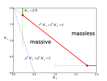
Figure 2: (Color online). Diagram showing the effect of commensurate densities (see text for discussion) in the special case of $n_{\uparrow}=1/3$, $n_{\downarrow}=2/3$, i.e. $p=2$ and $q=r=l=1$. For $2-2/9<K_{\downarrow}<2/9$ the interaction with the lattice leads to a formation of a ’trimer crystal’ state. For larger(smaller) values of $K_{\downarrow}$ the system has a phase transition from a massless phase into a Mott insulator of $\uparrow$($\downarrow$)-component. The ’trimer’ operator $\cos{2(2\phi_{\uparrow}-\phi_{\downarrow})}$ is always subdominant.

In the following, for sake of simplicity, we assume equal velocities of the two-components and drop the $\mathcal{H}_{1}$ term. The dominant instability of the massless theory $\mathcal{H}_{0}(\phi_{\uparrow})+\mathcal{H}_{0}(\phi_{\downarrow})$ is due to the operator with largest positive scaling dimension. Depending on the values of $K_{\uparrow}$ and $K_{\downarrow}$, the following inequalities define which of the operators (45)–(48) is relevant:

$$p^{2}K_{\uparrow}+q^{2}K_{\downarrow} \leqslant 2\;,$$ (49)

$$r^{2}K_{\uparrow}+l^{2}K_{\downarrow} \leqslant 2\;,$$ (50)

$$(pl+qr)^{2}K_{\downarrow} \leqslant 2\;,$$ (51)

$$(pl+qr)^{2}K_{\uparrow} \leqslant 2\;,$$ (52)

respectively. In Figs. 2 and 3 we plot the $(K_{\uparrow},K_{\downarrow})$ diagrams corresponding to Eqs. (49)–(52) for two values of the densities. We see that which instability takes place depends on the values of the bare Luttinger parameters $K_{\uparrow}$ and $K_{\downarrow}$, and thus on microscopic details of an underlying lattice model. Numerically, a crystal phase has been reported Keilmann2009 in a two-component bosonic Hubbard model and a similar result is presented in the fermionic counterpart in Sec. III.6 for the commensurabilities discussed in Fig. 2. These phases do correspond to the locking of several combinations of the modes according to Eqs. (45)–(48) but they are achieved for very large asymmetry. Consequently, the above criteria (49)–(52) determined for equal velocities are not directly applicable in these situations. The quantitative predictions of (49)–(52) could be relevant to the case of strongly renormalized $K_{\sigma}$, for instance with long-range intra-species interactions.

A striking feature of the phase diagrams 2 and 3 is the appearance of the multicritical points where several instabilities compete. In the above treatment we have only considered an effect of various operators (45)–(48) alone. An interplay between different operators is non-trivial and may lead to consequences not captured by the simple power counting of Eqs. (49)–(52). Hence, applicability of the above analysis in the vicinities of the multicritical points is not granted. There are several possible scenarios of the phase transitions at such multicritical points. For one thing, it is easy to construct fine-tuned theories where two continuous transitions occur simultaneously. An other possibility is a first order transition, as been observed in numerical simulations of higher-dimensional bosonic systems Kuklov2004 . Detailed analysis of these multicritical points is beyond the scope of the present paper.

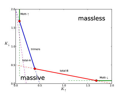
Figure 3: (Color online). Same as Fig. 2 for $n_{\uparrow}=1/5$, $n_{\downarrow}=2/5$. In this case, Eqs. (43)–(44) allow two sets of solutions: (A) $l=1$ and $r=3$, and (B) $l=2$ and $r=1$, with $p=2$ and $q=1$ in both cases. Solution (A) is always subdominant, while (B) dominates in the window $2/5<K_{\downarrow}<2/25$. For $48/25<K_{\downarrow}<2/5$, the dominant instability is the formation of a Luttinger liquid of trimers.

III Trimer formation in the 1D asymmetric Hubbard model

In this second part, we study the emergence of a trimer phase on a particular microscopic model : the 1D asymmetric attractive Hubbard model. After defining the model and providing its phase diagram as a function of the parameters, we discuss some limitations of the bosonization approach to this model and an alternative phenomenological description that completes the interpretation of the obtained data.

III.1 Model and qualitative aspects

We consider two species of fermions which internal degree of freedom is denoted by a spin index $\sigma$. They hop on a lattice with a spin-dependent amplitudes $t_{\sigma}$ (which would experimentally corresponds to different optical lattices for each species) and interact locally only in the inter-species channel with a Hubbard term $U$ which we take negative, as suggested by the arguments of Sec. II and as a natural choice to favor bonding between particles. The Hamiltonian is then :

$$\mathcal{H}=-\sum_{i,\sigma=\uparrow,\downarrow}t_{\sigma}[c^{{\dagger}}_{i+1,\sigma}c_{i,\sigma}+\text{h.c.}]+U\sum_{i}n_{i,\uparrow}n_{i,\downarrow}\;.$$ (53)

One of the key parameter for the physics is the ratio between the hoppings $\eta=t_{\downarrow}/t_{\uparrow}$. In order to have the possibility of forming trimers, we take the commensurate condition $2n_{\uparrow}=n_{\downarrow}$ but the total density $n$ varies freely and is another important parameter of the physics. Using the notations of Sec. II, we thus have $p=2$ and $q=1$ (the simplest new combination one can have). The Fermi momenta are $k_{\sigma}=\pi n_{\sigma}$ and free fermions Fermi velocities read $v_{\sigma}=2t_{\sigma}\sin(\pi n_{\sigma})$. Since $n_{\downarrow}\leq 1$, the maximum total density one can have for this commensurability is $n=3/2$.

The above Hamiltonian has been widely studied in the case of balanced Giamarchi1995 and imbalanced densities Yang2001 but the special commensurability where trimers emerge has only been investigated for one set of data in Ref. Burovski2009, , showing that the pairing correlations were indeed suppressed, in agreement with the bosonization approach. When the asymmetry is very large, one species behaves quasi-classically (they get localized) and the model is in the regime of the Falicov-Kimball (FK) model Falicov1969 where there exists a lot of quasi-degenerate states at low-energies, analogue to a phase separation regime. We expect generically a first-order transition to this segregated (or demixed) phase when lowering $\eta$ in the phase diagrams. The FK regime can display rather rich physics recently investigated in Ref. Barbiero2010, and which will not be analyzed here : our aim is only to draw the boundary of this regime. Numerically, the transition to the FK is rather sharp and all observables clearly display segregation. For $\eta=1$, the arguments of Sec. II suggest that the two-mode regime will be generically realized. Qualitatively, in a strong-coupling picture where two spin-$\downarrow$ fermions are localized on neighboring sites, the delocalization of a spin-$\uparrow$ electron on these sites will be favored by attractive interactions, forming a very local trimer state. This picture will be correct at small enough densities and actually not too large $U$ and too small $\eta$, otherwise such bound states will agglomerate with other spin-$\uparrow$ and $\downarrow$ fermions, leading to the FK regime. We thus expect the formation of the trimer phase in the vicinity of the FK but at both finite $U$ and finite $\eta$. Within the framework of Sec. II and considering that the starting point of bosonization are free fermions, the ratio between the velocities $\nu=v_{\downarrow}/v_{\uparrow}=2\eta\cos(\pi n/3)$ supports that small $\eta$ clearly favors the formation of trimers while small densities should not.

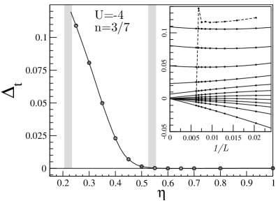
Figure 4: Opening of the trimer gap increasing mass asymmetry (lowering $\eta=t_{\downarrow}/t_{\uparrow}$) for a fixed interaction and density. The magnitude of the gap (in units of $t_{\uparrow}$) is small in comparison to $U$ and $t_{\uparrow}$. The grey areas are estimates of the transition points. Inset: finite size extrapolations of the gap. The upper dashed curve shows the behavior for $\eta=0.2$ when entering in the FK regime.

III.2 Phase diagrams

The phase diagrams of model (53) are numerically determined using standard DMRG with open-boundary conditions (OBC) and keeping up to $M=2000$ states. In order to discriminate between the different possible regimes, we use both “global” probes and local observables and correlation functions. Among “global” probes, one can use the trimer gap $\Delta_{\text{t}}$ associated with the formation of the bound state. It can be defined following Ref. Orso2010, as:

$$\begin{split}\Delta_{\text{t}}=&E_{0}(N_{\uparrow}+1,N_{\downarrow}+1)+E_{0}(N_{\uparrow},N_{\downarrow}+1)\\ &-E_{0}(N_{\uparrow}+1,N_{\downarrow}+2)-E_{0}(N_{\uparrow},N_{\downarrow})\;,\end{split}$$ (54)

with $E_{0}(N_{\uparrow},N_{\downarrow})$ the ground-state energy with $N_{\uparrow},N_{\downarrow}$ fermions. Results as the function of the asymmetry $\eta$ for an incommensurate density $n=3/7$ and large interaction $U=-4t_{\uparrow}$ have been extrapolated to the thermodynamical limit and are given in Fig. 4. The slow opening of the trimer gap is qualitatively compatible with the sine-Gordon behavior of Sec. II although the transformation is not directly applicable for any $\eta$. Notice that the whole system remains gapless. The slow opening of the gap makes it difficult to precisely locate the transition point. In such situation, a usual approach would be to use the prediction on the critical Luttinger parameter $K_{a}=K_{a}^{c}$ at the transition point. Furthermore, the determination of $K_{a}$ using correlators in the two-mode phase is very difficult as it would require to know, and then to disentangle, the complicated expression of the exponents as a function of $K_{a}$ and $K_{b}$ to extract them independently.

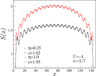
Figure 5: (Color online). Examples of fits of the entanglement entropy in the two-mode and single-mode phases using Eq. (55). It shows a clear quantitative difference with respectively $c\simeq 2$ and $c\simeq 1$, as expected.

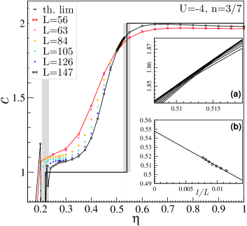
Figure 6: (Color online). Central charge $c$ obtained from fits as in Fig. 5 as a function of the asymmetry $\eta$ for $U=-4t_{\uparrow}$ and $n=3/7$. The stair-like behavior with increasing system size $L$ allows an efficient determination of the transition. In the Falicov-Kimball regime (left), fits give $c\simeq 0$ or irrelevant numbers. (a) Zoom of the $c(L)$ curves in the crossing region illustrating the extraction of crossing points between successive sizes. (b) Tentative finite-size extrapolation of the crossing points $\eta_{c}(L)$.

Therefore, we use another global approach to the distinction between the two-mode and single-mode phases, which is particularly well-suited for this model, and more generally in a similar context. Using universal results on the entanglement entropy (EE), the central charge $c$ of the model can be extracted which directly gives access to the number of bosonic modes, without further information on their nature. Hence, we expect $c=2$ in the two-mode regime while $c=1$ in the single-mode trimer phase. This stair-like expectation in the thermodynamical limit will be smoothed out by finite-size effects. The central charge is obtained on finite-systems using the following ansatz for the EE between a left block of size $x$ and the right block of length $L+1-x$ with OBC:

$$S(x)=\frac{c}{6}\ln d(x|L+1)+A\,t(x)+B\;,$$ (55)

where $d(x|L)$ is the cord function

$$d(x|L)=\frac{L}{\pi}\sin\left(\frac{\pi x}{L}\right)\;,$$ (56)

and $t(x)$ is the local kinetic energy on bound $(x,x+1)$ (obtained numerically), and $A,B$ are fitting parameters. The first log term is the leading and universal one Calabrese2004 while the second accounts for finite-size oscillations due to OBC and which can have a significant magnitude Laflorencie2006 ; Roux2009 . It is thus essential to take them into account to improve the quality of the fits. In the end, there are only three parameters in the procedure and typical examples in both the two-mode and single-mode phases are given in Fig. 5. Systematic fits on finite-size systems provide an estimate of $c$ as a function of the parameters. As seen in Fig. 6, the $c(L)$ curves crosses around the transition point. Although we do not have any quantitative prediction for the finite-size corrections of $c(L)$ obtained in this way, we can argue that if $L$ is smaller than the correlation length associated with the trimer gap, $c(L)$ will be larger than one as the system is effectively in a two-mode regime. Thus, $c(L)$ should decrease with $L$ towards one in the single-mode phase, as observed. In the two-mode phase, there is no obvious discussion : we only expect that the larger the system, the better the agreement with the continuous limit. One can also check the effect of the number of kept states on the fits and see that they don’t have the dominant effect in this model which converges well numerically. We have estimated the transition point by extrapolating the crossing points between successive sizes (see Fig. 6(a)) as a function of the inverse size (see Fig. 6(b)). From this approach and the opening of the gap, we get a critical value $\eta_{c}\simeq 0.54\pm 0.02$ for the mass asymmetry on this cut. Although the gap is rather small, the trimer region appears to be rather wide.

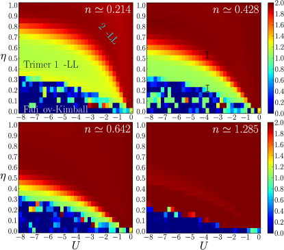
Figure 7: (Color online). Maps of the central charge $c$ vs interaction $U$ and asymmetry $\eta$ for a system with $L=112$ at four different densities. For $n=3/7\simeq 0.428$, the lines with error bars are the ones estimated from Figs. 4 and 6. The $\eta=0$ cuts correspond to data obtained with a very low but non-zero value $\eta=0.005$.

Using the central charge calculation, one can map out the phase diagram in the $(\eta,U)$ plane for a fixed density, or in the $(\eta,n)$ plane for a fixed interaction $U$. Results are gathered in Fig. 7 and 8 respectively. These diagrams display bare data for a given system with a rather large size $L=112$ and the previous estimate of the cut is given as error bars. These diagrams show that a wide trimer phase can be achieved at large enough interactions, small enough $\eta$, as expected, and also that low densities strongly favors their formation. At large densities $n\simeq 1.3$, the trimer region vanishes within our grid resolution so that it is at most confined to a very tiny region between the two-mode phase and the FK regime. While the large-$|U|$ situation is rather clear, the competition between the three regimes at small $U$ is more involved. Indeed, two scenarios can occur in the $(\eta,U)$ plane: either the trimer phase always separates the FK and two-mode regimes, corresponding to two boundaries starting from the $(\eta=0,U=0)$ corner, or there is a critical $|{U}|$ above which the trimer phase emerges, corresponding to a tricritical point $(\eta_{c},U_{c})$. We could not numerically discriminate between both scenarios, but we do find a small trimer region at relatively small $U$s ($U\simeq-1\,t_{\uparrow},-2\,t_{\uparrow}$) for most densities : we do not have evidence for a tricritical point with a large $U_{c}$. As the density plays a central role in the stabilization of the trimer phase, we give in Fig. 8 the central charge map for a fixed interaction $U=-4t_{\uparrow}$ as a function of the total density $n$ and mass asymmetry. A similar question about a intervening trimer phase between the two-mode and the FK regimes can be raised. While the two-mode and FK are clearly separated at small densities, we found that if a trimer intermediate phase exists at large densities up to the $(\eta=0,n=1.5)$ point, its extension will be particularly small (not seen within our numerical calculations). In addition to the three main phases, commensurability effects are also present in this diagram. When the maximum density $n=1.5$ is reached, the $\downarrow$-band is completely filled while the $\uparrow$-band is half-filled, leading to a single-mode phase well-captured by the central charge approach. Lastly, as it will be discussed in Sec. III.6, a crystal phase (fully gapped) exists for the commensurate density $n=1$ at very small $\eta$ and is pointed on Fig. 8. Other commensurabilities could yield additional crystal-like phases in this diagram but this is beyond the scope of this study.

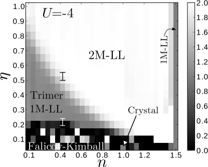
Figure 8: Map of the central charge $c$ vs asymmetry $\eta$ and total density $n$ for fixed interaction $U=-4t_{\uparrow}$ on a system with $L=128$. The lines with error bars are the ones estimated from Figs. 4 and 6.

III.3 Observables and effective behavior of the trimer liquid

In this section, we give the behavior of several observables in order to see how they are affected by the entrance into the trimer phase or the FK regime and, as well, to investigate the effective behavior of the trimer fermion.

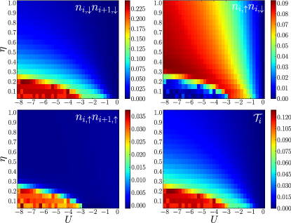
Figure 9: (Color online). Maps of averaged local quantities in a system with $L=56$ at total density $n=3/7\simeq 0.428$. The non-interacting expectation ($U=0$ line) has been subtracted in order to unveil the effect of the interaction.

III.3.1 Local observables

First, we select a set of local correlators (living on sites or on bonds) which illustrate the phenomenological picture of the different parts of the phase diagram. We compute the local double occupancy $\langle{n_{i,\uparrow}n_{i,\downarrow}}\rangle$, the trimer local operator as $\mathcal{T}_{i}=\frac{1}{2}(\langle{n_{i,\uparrow}n_{i,\downarrow}n_{i+1,\downarrow}}\rangle+\langle{n_{i+1,\uparrow}n_{i,\downarrow}n_{i+1,\downarrow}}\rangle)$ (since the light particle is in principle delocalized above two heavier), and the density correlators $\langle{n_{i,\uparrow}n_{i+1,\uparrow}}\rangle$ and $\langle{n_{i,\downarrow}n_{i+1,\downarrow}}\rangle$. This choice of local correlators is well suited to a strong-coupling picture as pairs or trimers should in principle correspond to a narrow bound-state, spread over only a few lattice sites. These local correlators should then pick up a reasonable weight of the local bound-state. The results are averaged over all lattice sites and plotted in Fig. 9. The expectation value at $U=0$ has been subtracted so that the reference state is the free fermions limit at a given $\eta$ (the pairing or trimer local correlators defined above are obviously non-zero even in the free fermions limit). Fig. 9 display behaviors in qualitative agreement with the picture we have on the trimer formation : the ${\uparrow\uparrow}$ density correlator is nearly zero everywhere but in the FK regime, signaling phase separation. On the contrary ${\downarrow\downarrow}$ density correlator increases significantly in the region corresponding to the trimer phase, surrounding the FK pocket, and together with the local trimer density $\mathcal{T}_{i}$. Lastly, we see that the double occupancies, or pairs, acquire a strong weight with negative $U$ everywhere in two-mode and single-mode regions : they are either “independent” or embedded in the trimer bound-state. Their coherence can yet be probed only by measuring correlations as discussed below.

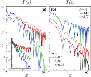
Figure 10: (Color online). Behavior of (a) pairing and (b) trimer correlations when lowering $\eta$ and entering the trimer phase along a cut at $U=-4t_{\uparrow}$ in the phase diagram (absolute values are displayed). The Inset of (a) shows the same data but in log-linear scale to highlight the exponential decay.

III.3.2 Pairing and trimer correlations, effective behavior of the trimers

We now turn to the behavior of correlation functions across the phase diagram. From Sec. II.3, and as already observed for a particular point in Refs. Burovski2009, ; Orso2010, , the pairing correlations change from algebraic to exponential decay when entering into the trimer phase. These correlations are here computed in the singlet channel and for local pairs $\hat{P}_{i}=c_{i,\uparrow}c_{i,\downarrow}$. In addition, we compute the trimer correlator using the local trimer operator $\hat{T}_{i}=c_{i,\uparrow}c_{i,\downarrow}c_{i+1,\downarrow}$ defined on neighboring sites. The associated correlation functions $P(x)=\langle{\hat{P}^{\dagger}_{i}\hat{P}_{i+x}}\rangle$ and $T(x)=\langle{\hat{T}^{{\dagger}}_{i}\hat{T}_{i+x}}\rangle$ are computed with $i$ taken at the center of the chain. Increasing the mass asymmetry along the same cut at $U=-4t_{\uparrow}$ as in previous figures, the suppression of pairing correlations is clearly seen in Fig. 10(a). On the contrary, trimer correlations, which are subdominant in the two-mode regime, are boosted by smaller $\eta$, both in amplitude (as for the local correlators previously evoked) and in the decay exponent which gets smaller (see Fig. 10(b)). Notice that the wave-vector is the same for both correlators since $k_{\downarrow}-k_{\uparrow}=k_{\uparrow}=\pi n/3$ for this commensurability. We have tentatively extracted the decay exponents of both correlators by fitting the functions using a power-law modulated by a cosine oscillations. The correlation length $\xi$ of the pairing correlator in the trimer phase is obtained using an exponential envelope $e^{-x/\xi}$. The results are gathered in Fig. 11, showing the evolution in both phases. We must stress that the data computed on a finite-size system display a transition at a lower $\eta$ than in the thermodynamical limit. From Sec. II.3, we expect that the decay exponent of the trimer propagator is of the form $(K_{\text{eff}}+K_{\text{eff}}^{-1})/2$ while the $\uparrow$-density correlations have a decay exponent of $2K_{\text{eff}}$. A first consequence is that the trimer exponent should always be larger than one which is not reproduced for the lowest $\eta$s, and which we attribute to numerical inaccuracies of the fits of trimer correlations. Besides, inverting $(K_{\text{eff}}+K_{\text{eff}}^{-1})/2$ to get $K_{\text{eff}}$ is subjected to strong errors when $K_{\text{eff}}\simeq 1$ and does not tell whether $K_{\text{eff}}>1$ or $K_{\text{eff}}<1$ which is essential for the effective behavior of the trimers. In order to get a better estimate of $K_{\text{eff}}$, we rather use Friedel oscillations of the $\uparrow$-density operator which decay exponent $\alpha$ is equal to $K_{\text{eff}}$ in the trimer phase according to Sec. II.3.

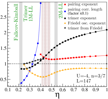
Figure 11: (Color online). Comparison of the decay exponents of pairing and trimer correlations. The correlation length of pairing correlation (in units of the lattice spacing) is given in the trimer phase. The strong grey areas are the previous estimates of the transition points while the light maroon area illustrates the location of the transition on the $L=147$ finite-size system under study. The exponent of the Friedel oscillations of $n_{\uparrow}$ is also displayed, together with the expected trimer exponent derived from it (see text for discussion).

Even though the approach of Sec. II.3 is not applicable for most parameters, the fact that there exists an effective Luttinger exponent $K_{\text{eff}}$ describing the physics of the fermionic trimer with a propagator $(K_{\text{eff}}+K_{\text{eff}}^{-1})/2$ and with Friedel oscillations with $K_{\text{eff}}$ is more general : the limitation of the bosonization approach is rather that $K_{\text{eff}}$ will not take the form of Eq. (40). Local observables are believed to have less numerical errors associated with a finite number of kept states than correlations White2007 . Thus, we fit the Friedel oscillations of the $\uparrow$-density using the following symmetric ansatz

$$n_{i,\uparrow}=n_{0}+A\frac{\cos\,q(i-\frac{L+1}{2})}{[d(i|L+1)]^{\alpha}}$$ (57)

with $1\leq x\leq L$ and only four fitting parameters $n_{0}$, $A$, $q$ and $\alpha$ . In the trimer phase, we expect $\alpha=K_{\text{eff}}$. Some typical fits are plotted in Fig. 12(a). From them, we extract the decay exponent $\alpha$ and plot it on Fig. 12(b) as a function of the total density. A cusp is found around $n\simeq 0.6$ signaling the transition from the two-mode regime to the trimer phase. We have seen that a low density favors the formation of the trimer phase. This figure shows that, in the trimer phase, we have $K_{\text{eff}}<1$ for the larger densities, corresponding to a repulsive effective interaction between trimers (dominant CDW order of trimers). We observe that the exponent increases with decreasing density, compatible with the fact that at low densities in the trimer regime, the trimers should be close to free spinless fermions having $K_{\text{eff}}\simeq 1$. Bare data for the smallest density on a system with $L=144$ even display an exponent $K_{\text{eff}}\simeq 1.2$ larger than one.

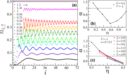
Figure 12: (Color online). (a) Typical Friedel oscillations of the $\uparrow$-density for $U=-4t_{\uparrow}$, $\eta=0.3$ and $L=144$ for various densities $n$. Full lines are fits using Eq. (57). (b) Decay exponents obtained from the fits as a function of the density. The cusp at $n\simeq 0.6$ roughly corresponds to the transition from the two-mode to the single-mode regime. (c) Large exponents at low densities, close to the FK regime when lowering $\eta$ : increasing the size tends to reduce the exponent below one.

Interestingly, the trimers in this model are necessarily objects with a finite extension of at least two sites and two close trimers may have the possibility to overlap by delocalizing their $\uparrow$ electrons. The distance dependence and sign of the effective interaction between trimers is non-trivial – a perturbation theory to derive it looks challenging as it involves many sites and degrees of freedom. Yet, since the trimer phase is found close to the FK regime, we can expect the effective interaction to become attractive close to this boundary, leading to $K_{\text{eff}}>1$. Such physics would correspond to a superfluid phase of trimers. This would be physically very remarkable since the microscopic Hamiltonian (53) would contain both the formation of bound-states, or molecules, and their effective superfluid behavior. However, the behavior close to a phase separation at small densities is numerically involved. Indeed, increasing the system size $L$ shows that $\alpha$ actually tends to decrease below one, as reported in Fig. 12(c), or one enters the FK regime for larger sizes. We did not find clear evidence of a stabilization of $K_{\text{eff}}>1$ in the thermodynamical limit and understand the observed $K_{\text{eff}}>1$ as finite size effects. A superfluid droplet picture can be qualitatively put forward. Starting from the FK regime and looking at the local density pattern, one sees that the fermions are clustered into droplets while other parts of the box are empty. Approaching the trimer phase from the FK regime tends to increase the size of these droplets to gain kinetic energy. When a box confinement is present (finite system with OBC), it naturally favors the overlap between trimers, by depleting the edges, and can prevent the droplet to form (for instance if their typical size is larger than the box size). Increasing further the size of the box (at constant density) can lead to droplets formation. This is a possible interpretation of the data observed in Fig. 12(c). In addition, we must stress that there is a lot of competing low-energy states in the FK regimes so DMRG, as an essentially variational methods, can be trapped into metastable states. Even though the thermodynamical limit is unclear, it is experimentally motivating to have signatures of superfluidity on mesoscopic confined systems as one has in cold-atoms setups. We further mention that a recent careful study of the t-J model on a chain Moreno2010 which could qualitatively contain a similar phenomenon as pair-clustering did not find evidences for such clustering.

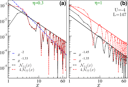
Figure 13: (Color online). Density correlations in (a) the trimer phase and (b) the two-mode phase with $n=3/7$.

III.3.3 Locking between density correlations

Lastly, the comparison of density-density correlations in the $\uparrow$ and $\downarrow$ channels is another interesting point of this model. In fact, the bosonization results of Sec. II.3 predicts that the exponent of $\mathcal{N}_{\uparrow\uparrow}(x)$ should be four times larger than the exponent of $\mathcal{N}_{\downarrow\downarrow}(x)$ (if both remains smaller than two), and that the dominant wave-vector should differ by a factor two. Numerically, the typical behavior for a rather large interaction $U=-4t_{\uparrow}$ is given on Fig. 13 for two values of the asymmetry $\eta$ in the single-mode and two-mode regimes. We see that in the two-mode phase (Fig. 13(b)), the two fluctuations have a slightly different exponent, that the amplitude are quite different (including the natural factor four). Yet, the dominant wave-vectors are both $2k_{\uparrow}=k_{\downarrow}$. In the trimer phase, the disagreement with the bosonization picture is even worse since the two densities are locked together, and nearly identical (Fig. 13(a)). This latter fact cannot be explained by the $1/x^{2}$ decay since the leading term is the oscillating one, with an exponent clearly smaller than two. It is yet physically not surprising in the strong coupling picture of Fig. 1 : trimers are local bound-states separated by the typical distance $1/n_{\uparrow}=2\pi/2k_{\uparrow}$ which does correspond to the $2k_{\uparrow}$ fluctuations but cannot be accounted by any of the harmonics for the $\downarrow$-density operator of Eq. (3) (we work at an incommensurate filling). This short-distance binding cannot be captured by the bosonization results of Sec. II but a phenomenological Bose-Fermi approach described in the next section can account for this strong-coupling regime. Lastly, the same comment can be made on Friedel oscillations on the $\downarrow$-component : they are locked to the $\uparrow$-component in the strong-coupling picture. One might argue that there could be a crossover from the weak-coupling to strong-coupling picture of Fig. 1 as $|U|$ increases, so that the bosonization results could be valid in the small $U$s region. However, the trimer region is very sharp at small $U$s and we could not find evidence for such a weak-coupling behavior in our numerical data, although we cannot exclude such a possibility.

III.4 Phenomenological Bose-Fermi picture at large $|{U}|$

We here propose a simple picture that reconciles the numerical observation and a bosonization approach at the prize of a strong assumption, physically reasonable at large negative $U$, but difficult to justify rigorously starting from the microscopic model. This picture has been for instance proposed at large interaction and low-density limit Iskin2008 . Bose-Fermi mixtures of 1D models have extensively studied in recent years Cazalilla2003 ; Pollet2006 ; Mathey2007 ; Mathey2007a ; Hebert2008 ; Barillier-Pertuisel2008 ; Rizzi2008 ; Mering2008 ; Marchetti2009 ; Crepin2010 ; Orignac2010 and a similar picture emerges in certain regimes of three-component Fermi-gases Luscher2009 . When $|{U}|$ is large, $\uparrow$ and $\downarrow$ fermions naturally form onsite pairs which are effectively hard-core bosons which we label $b$. We phenomenologically assume that the system is equivalent to a Luttinger liquid of hard-core bosons with density $n_{b}=n_{\uparrow}$, an effective velocity $v_{b}$ and Luttinger parameter $K_{b}$, while the remaining unpaired $\downarrow$ fermions behave as a Luttinger liquid of fermions labeled by $f$ and with parameters $n_{f}$, $v_{f}$ and $K_{f}$. These two Luttinger liquids interact through an effective interaction which will contain terms such as

$$\int\!dx\,\cos{\left[2\pi(n_{f}-n_{b})x-2(\phi_{f}-\phi_{b})\right]}\;,$$ (58)

which have the tendency to lock the fields $\phi_{f}$ and $\phi_{b}$ together (with $\langle{\phi_{f}}\rangle=\langle{\phi_{b}}\rangle$ for attractive interaction), provided $n_{f}=n_{b}$. Such an effect has already been discussed in the context of Bose-Fermi mixtures Rizzi2008 ; Marchetti2009 . Clearly, the latter relation is the same as the trimer commensurability condition $n_{\downarrow}=2n_{\uparrow}$ (because bosons carry two particles) so that the formation of trimer is now interpreted as a bound-state between the bosons and the fermions. Following the same reasoning as in Sec. II.2, we can introduce a general transformation of the $b/f$ fields into two new fields $c/d$ where $\phi_{c}=(\phi_{f}-\phi_{b})/\sqrt{2}$. Writing the matrix transformation from the $r=c,d$ to the $s=b,f$ as $\mathfrak{p}_{rs}$ for the $\phi$s and $\mathfrak{t}_{rs}$ for the dual $\theta$s, we have

$$\mathfrak{t}_{cf} =\frac{1}{\sqrt{2}}\;, \mathfrak{t}_{cb} =-\frac{1}{\sqrt{2}}\,.$$ (59)

which is slightly different from Eq. (19). Yet, the 2$k_{F}$-like fluctuating part of the density correlators for the fermions and the bosons will have the leading contributions (dropping the $x^{-2}$ terms) :

$$\mathcal{N}_{ff}(x)\sim\frac{\cos(2k_{f}x)}{x^{2\mathfrak{p}_{df}^{2}K_{d}}}\;,$$ (60)

$$\mathcal{N}_{bb}(x)\sim\frac{\cos(2k_{b}x)}{x^{2\mathfrak{p}_{db}^{2}K_{d}}}\;,$$ (61)

which have both the same wave-vector associated with the Fermi levels $k_{f}=k_{b}=k_{\uparrow}$ and same decay exponents since $\mathfrak{p}_{df}=\mathfrak{p}_{db}$ from the canonical transformation relations. In this picture, the trimer is simply a bound-state between the bosons and the fermions so its propagator reads

$$T(x) \sim e^{ik_{f}x}e^{i\theta_{b}}e^{i(\theta_{f}-\phi_{f})}$$ (62)

$$\sim e^{ik_{\uparrow}x}e^{i[(\mathfrak{t}_{df}+\mathfrak{t}_{db})\theta_{d}+(\mathfrak{t}_{cf}+\mathfrak{t}_{cb})\theta_{c}-\mathfrak{p}_{df}\phi_{d}-\mathfrak{p}_{cf}\phi_{c}]}\,.$$ (63)

From Eq. (59) and the determinant of the transformation matrix, which gives that $\mathfrak{t}_{df}+\mathfrak{t}_{db}=1/\mathfrak{p}_{db}=1/\mathfrak{p}_{df}$, we obtain that the propagator is of the spinless fermionic type with an effective Luttinger parameter $K^{\prime}_{\text{eff}}=\mathfrak{p}_{df}^{2}K_{d}$. Clearly, both the $f$-fermions and $b$-bosons propagators become short-range, the latter corresponding to the pairing correlations in the native fermionic model. Consequently, we recover the physics of the trimer phase developed in Sec. II, with a better agreement with the numerical observations in the strong coupling regime. However, splitting the initial gas of $\downarrow$ fermions into two parts can only be done phenomenologically and could be questionable in a microscopic derivation. This highlights the limitation of the bosonization approach of Sec. II at short distances (high energies).

III.5 Possible observation of the trimer phase in the presence of parabolic confinement

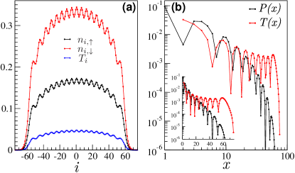
Figure 14: (Color online). Realization of the trimer phase in a trapped configuration with parameters $U=-4t_{\uparrow}$, $\eta=0.3$, $\omega=0.002\sqrt{t_{\uparrow}}$, and $N=51$ fermions. (a) Local densities profiles. (b) Correlation functions from the center of the trap. Inset: same in log-linear scale.

In this section, we briefly discuss the condition to favor the trimer phase in the presence of a parabolic confinement, as used in cold-atoms experiments. Our goal is only to exhibit some parameters for which the trimer phase is stabilized and to give some qualitative comments. The trapping potential is taken into account by adding the quadratic term

$$\mathcal{H}_{\text{trap}}=\frac{1}{2}\omega^{2}\sum_{i}(i-i_{0})^{2}$$ (64)

to Eq. 53, with the trapping frequency $\omega$ and the center of the lattice $i_{0}=(L+1)/2$. According to a local-density approximation (LDA) picture and using the phase diagram of Fig. 8, the trimer phase is likely to be found at small enough densities and not too small $\eta$ to prevent the occurrence of the FK regime. However, we find that the average density of the trapped system is strongly dependent on the Hamiltonian parameters. At fixed number of particles $N$ and trap size $\omega$, changing $U$ and $\eta$ strongly affects the radius of the cloud and the density in the middle. We only exhibit in Fig. 14 parameters for which the main features of the trimer phase are reproduced in the presence of a parabolic confinement. The density profiles of Fig. 14(a) illustrate the locking of the $\uparrow$ and $\downarrow$ densities (up to exactly a factor two), and the emergence of an appreciable density of local trimers (each local maximum roughly corresponding to a trimer). In Fig. 14(b), the pairing and trimer correlations are strongly different from that of a superfluid phase : we have dominating trimer correlations and exponential pairing correlations as in the homogeneous counterpart. In agreement with a LDA picture, since we have seen that $K_{\text{eff}}$ decreases with density, the trimer correlations are boosted at long distances. Similarly, the pairing correlations decrease slightly faster then an exponential close to the edge of the cloud. These results are encouraging in the perspective of a possible achievement of the trimer phase in actual experiments.

III.6 Observation of a crystal of trimers

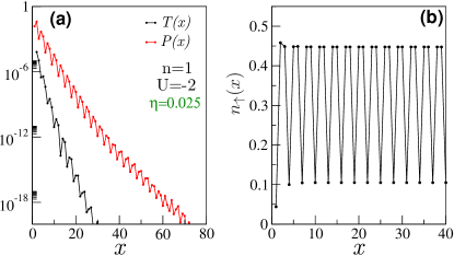
Figure 15: (Color online). Observation of the crystallization of trimers in the commensurability situation of Fig. 2 ($n=1$). (a) the short-range behavior of both pairing and trimer correlations. (b) ordering of the local density $n_{\uparrow}$ with the expected period of three sites.

According to the analysis of Sec. II.4, a crystalline phase of trimers can occur in this lattice model when the total density $n$ is commensurate. Evidence of this scenario together with a phase diagram for $n=1$ has been proposed in Ref. Keilmann2009, in the case of a mixture of two-component bosons, for large enough asymmetry. As the order parameter (the density) associated with this transition is independent of the statistics, we expect a similar scenario (see Sec. II.4) and a similar location of the transition in the fermionic version of the model under study. Indeed, we give in Fig. 15 an example of the crystal phase. Notice that very small $\eta$ are required to stabilize such a phase. We have not investigated the extension of the phase which should rather be small on the scale of the phase diagram of Fig. 8 and its neighboring phases which could be either the two-mode LL or the trimer phase. A crude argument can be proposed to understand this crystallization within the Bose-Fermi picture of Sec. III.4 : when the mass asymmetry is very large (very small $\eta$), it is reasonable to say that the mass of the boson will be essentially the one of the heaviest particle, which is the same as the unpaired fermions so that $v_{f}\simeq v_{b}$. In terms of commensurability effects, one has $n_{f}=n_{b}=n/3$ so that standard umklapp terms at $2\pi(n_{f}+n_{b})=4\pi/3$ do not account for the crystallization. One rather has to look for higher order terms with commensurabilities such as $2n_{f}+n_{b}=n_{f}+2n_{b}=n=1$, which are typically associated with terms like

$$\int\!dx\,\cos{2(2\phi_{f}+\phi_{b})}\;,$$ (65)

in addition to the one of Eq. (58). Such term can lock the field $2\phi_{f}+\phi_{b}$ and make the system fully gapped. Lastly, we would like to stress that such commensurabilities are rather surprising in terms of the initial fermion densities as they belong to odd filling fractions $n_{\uparrow}=1/3$ and $n_{\downarrow}=2/3$.

IV Conclusions

In summary, the consideration of unusual commensurability conditions in density-density interactions for 1D two-component gases leads to a very rich physics with the possibility of building bound-states of $(p+q)$-particles as the leading order. Such a mode-locking mechanism can be described within the framework of Luttinger liquid theory which reveals the main ingredients to stabilize such a new phase. In particular, mass or velocity asymmetry is shown to drive efficiently the transition into the multimer phase. Novel fully gapped phases are proposed when taking into account umklapp couplings specific to lattice models at commensurate densities. These ideas are illustrated and confronted with the asymmetric 1D attractive Hubbard model for the special commensurability $2n_{\uparrow}=n_{\downarrow}$ for which the formation of trimers is found. The features of the phase diagram are computed, displaying the important role of the density in favoring the trimer phase. The effective behavior of trimers, which are effectively spinless fermionic objects, is very sensitive to the density and mass asymmetry. Although the model seems to have promising features to sustain a superfluid phase of trimers, we did not find clear evidence for it in the thermodynamical limit, while finite-size systems display a “superfluid droplets” physics. Notice that superfluidity of bound-states made of four fermions (quartets) can be achieved reliably in 1D with a four-color Hubbard model Capponi2008 ; Roux2009 . There, the bound-states are bosons which natural “free” regime (attained in the low-density limit) is a superfluid phase. A superfluid phase of trimers would in this respect be even more exotic but is in strong competition with phase separation. Lastly, we found that a trapping confinement supports the trimer phase for reasonably high densities and that surprising crystal phases can emerge at commensurate densities.

- (1) A. J. Leggett, Quantum Liquids: Bose Condensation and Cooper Pairing in Condensed-Matter Systems (Oxford University Press, 2006).
- (2) J. R. Schrieffer, Theory Of Superconductivity (Perseus Books, 1999).
- (3) T. Giamarchi and B. S. Shastry, Phys. Rev. B 51, 10915 (1995).
- (4) T. Giamarchi, Quantum Physics in one Dimension International series of monographs on physics Vol. 121 (Oxford University Press, Oxford, UK, 2004).
- (5) O. Mandel et al., Phys. Rev. Lett. 91, 010407 (2003).
- (6) E. Wille et al., Phys. Rev. Lett. 100, 053201 (2008); M. Taglieber, A.-C. Voigt, T. Aoki, T. W. Hänsch, and K. Dieckmann, Phys. Rev. Lett. 100, 010401 (2008).
- (7) S. Giorgini, L. P. Pitaevskii, and S. Stringari, Rev. Mod. Phys. 80, 1215 (2008).
- (8) K. Penc and J. Sólyom, Phys. Rev. B 41, 704 (1990).
- (9) D. Carpentier and E. Orignac, Phys. Rev. B 74, 085409 (2006).
- (10) I. Martin, Y. M. Blanter, and A. F. Morpurgo, Phys. Rev. Lett. 100, 036804 (2008); M. Killi, T.-C. Wei, I. Affleck, and A. Paramekanti, Phys. Rev. Lett. 104, 216406 (2010).
- (11) E. Braaten and H.-W. Hammer, Physics Reports 428, 259 (2006); E. Braaten and H.-W. Hammer, Annals of Physics 322, 120 (2007).
- (12) D. S. Petrov, Phys. Rev. A 67, 010703 (2003); M. Iskin, Phys. Rev. A 81, 043634 (2010); F. Alzetto, R. Combescot, and X. Leyronas, Phys. Rev. A 82, 062706 (2010).
- (13) J. Levinsen, T. G. Tiecke, J. T. M. Walraven, and D. S. Petrov, Phys. Rev. Lett. 103, 153202 (2009); F. Werner and Y. Castin, ArXiv e-prints, 1001.0774; D. Blume and K. M. Daily, Phys. Rev. Lett. 105, 170403 (2010); Y. Castin, C. Mora, and L. Pricoupenko, Phys. Rev. Lett. 105, 223201 (2010).
- (14) G. B. Partridge, W. Li, R. I. Kamar, Y. A. Liao, and R. G. Hulet, Science 311, 503 (2006); G. B. Partridge et al., Phys. Rev. Lett. 97, 190407 (2006); Y. an Liao et al., Nature 467, 567 (2010).
- (15) K. A. Muttalib and V. J. Emery, Phys. Rev. Lett. 57, 1370 (1986).
- (16) D. Loss and T. Martin, Phys. Rev. B 50, 12160 (1994).
- (17) M. A. Cazalilla and A. F. Ho, Phys. Rev. Lett. 91, 150403 (2003).
- (18) L. Mathey, D.-W. Wang, W. Hofstetter, M. D. Lukin, and E. Demler, Phys. Rev. Lett. 93, 120404 (2004).
- (19) M. A. Cazalilla, A. F. Ho, and T. Giamarchi, Phys. Rev. Lett. 95, 226402 (2005).
- (20) L. Mathey, Phys. Rev. B 75, 144510 (2007).
- (21) L. Mathey and D.-W. Wang, Phys. Rev. A 75, 013612 (2007).
- (22) W.-L. Lu, Z.-G. Wang, S.-J. Gu, and H.-Q. Lin, ArXiv e-prints, 0902.1021.
- (23) F. Crépin, G. Zaránd, and P. Simon, Phys. Rev. Lett. 105, 115301 (2010).
- (24) E. Orignac, M. Tsuchiizu, and Y. Suzumura, Phys. Rev. A 81, 053626 (2010).
- (25) A. M. Tsvelik, ArXiv e-prints, 1004.5092.
- (26) L. Pollet, M. Troyer, K. Van Houcke, and S. M. A. Rombouts, Phys. Rev. Lett. 96, 190402 (2006).
- (27) A. Mering and M. Fleischhauer, Phys. Rev. A 77, 023601 (2008).
- (28) G. G. Batrouni, M. J. Wolak, F. Hébert, and V. G. Rousseau, Europhys. Lett. 86, 47006 (2009).
- (29) B. Wang, H.-D. Chen, and S. Das Sarma, Phys. Rev. A 79, 051604 (2009).
- (30) E. Burovski, G. Orso, and T. Jolicœur, Phys. Rev. Lett. 103, 215301 (2009).
- (31) G. Orso, E. Burovski, and T. Jolicœur, Phys. Rev. Lett. 104, 065301 (2010).
- (32) C. Wu, Phys. Rev. Lett. 95, 266404 (2005); P. Lecheminant, E. Boulat, and P. Azaria, Phys. Rev. Lett. 95, 240402 (2005); S. Capponi, G. Roux, P. Azaria, E. Boulat, and P. Lecheminant, Phys. Rev. B 75, 100503 (2007); A. Rapp, G. Zaránd, C. Honerkamp, and W. Hofstetter, Phys. Rev. Lett. 98, 160405 (2007); P. Azaria, S. Capponi, and P. Lecheminant, Phys. Rev. A 80, 041604 (2009); T. Sogo, G. Röpke, and P. Schuck, Phys. Rev. C 81, 064310 (2010).
- (33) S. Capponi et al., Phys. Rev. A 77, 013624 (2008).
- (34) G. Roux, S. Capponi, P. Lecheminant, and P. Azaria, Eur. Phys. J. B 68, 293 (2009).
- (35) S. R. White, Phys. Rev. Lett. 69, 2863 (1992); S. R. White, Phys. Rev. B 48, 10345 (1993); U. Schollwöck, Rev. Mod. Phys. 77, 259 (2005).
- (36) F. D. M. Haldane, Phys. Rev. Lett. 47, 1840 (1981).
- (37) S. Engelsberg and B. B. Varga, Phys. Rev. 136, A1582 (1964).
- (38) P. Fulde and R. A. Ferrell, Phys. Rev. 135, A550 (1964); A. I. Larkin and Y. N. Ovchinikov, Sov. Phys. JETP 20, 762 (1965).
- (39) S. Lukyanov and A. Zamolodchikov, Nuclear Physics B 493, 571 (1997).
- (40) Ş. G. Söyler, B. Capogrosso-Sansone, N. V. Prokof’ev, and B. V. Svistunov, New J. Phys. 11, 073036 (2009).
- (41) T. Keilmann, I. Cirac, and T. Roscilde, Phys. Rev. Lett. 102, 255304 (2009).
- (42) A. Kuklov, N. Prokof’ev, and B. Svistunov, Phys. Rev. Lett. 92, 050402 (2004); E. K. Dahl, E. Babaev, S. Kragset, and A. Sudbø, Phys. Rev. B 77, 144519 (2008).
- (43) K. Yang, Phys. Rev. B 63, 140511 (2001); H. Hu, X.-J. Liu, and P. D. Drummond, Phys. Rev. Lett. 98, 070403 (2007); G. Orso, Phys. Rev. Lett. 98, 070402 (2007); A. E. Feiguin and F. Heidrich-Meisner, Phys. Rev. B 76, 220508 (2007); M. Tezuka and M. Ueda, Phys. Rev. Lett. 100, 110403 (2008); G. G. Batrouni, M. H. Huntley, V. G. Rousseau, and R. T. Scalettar, Phys. Rev. Lett. 100, 116405 (2008); A. Lüscher, R. M. Noack, and A. M. Läuchli, Phys. Rev. A 78, 013637 (2008); F. Heidrich-Meisner, G. Orso, and A. E. Feiguin, Phys. Rev. A 81, 053602 (2010).
- (44) L. M. Falicov and J. C. Kimball, Phys. Rev. Lett. 22, 997 (1969).
- (45) L. Barbiero et al., Phys. Rev. B 81, 224512 (2010).
- (46) P. Calabrese and J. Cardy, J. Stat. Mech. , P06002 (2004); P. Calabrese and J. Cardy, J. Phys. A 42, 504005 (2009).
- (47) N. Laflorencie, E. S. Sørensen, M.-S. Chang, and I. Affleck, Phys. Rev. Lett. 96, 100603 (2006); I. Affleck, N. Laflorencie, and E. S. Sørensen, J. Phys. A 42, 504009 (2009); J. Cardy and P. Calabrese, J. Stat. Mech. 2010, P04023 (2010).
- (48) S. R. White and A. L. Chernyshev, Phys. Rev. Lett. 99, 127004 (2007).
- (49) A. Moreno, A. Muramatsu, and S. R. Manmana, ArXiv e-prints, 1012.4028.
- (50) M. Iskin and C. A. R. Sá de Melo, Phys. Rev. A 77, 013625 (2008).
- (51) F. Hébert, G. G. Batrouni, X. Roy, and V. G. Rousseau, Phys. Rev. B 78, 184505 (2008).
- (52) X. Barillier-Pertuisel, S. Pittel, L. Pollet, and P. Schuck, Phys. Rev. A 77, 012115 (2008).
- (53) M. Rizzi and A. Imambekov, Phys. Rev. A 77, 023621 (2008).
- (54) F. M. Marchetti, T. Jolicœur, and M. M. Parish, Phys. Rev. Lett. 103, 105304 (2009).
- (55) A. Lüscher and A. Läuchli, ArXiv e-prints, 0906.0768.