Elastic fluctuations as observed in a confocal slice

Abstract

Recent confocal experiments on colloidal solids motivate a fuller study of the projection of three-dimensional fluctuations onto a two-dimensional confocal slice. We show that the effective theory of a projected crystal displays several exceptional features, such as non-standard exponents in the dispersion relations. We provide analytic expressions for the effective two-dimensional elastic properties which allow one to work back from sliced experimental observations to three-dimensional elastic constants.

Colloids Phonons or vibrational states in low-dimensional structures and nanoscale materials Lattice dynamics - Measurements

Optical techniques, including scattering and microscopy, have long been used to extract detailed static and dynamic information from soft condensed matter systems. They are in many ways complementary – scattering being most suitable for examining the fluctuations in Fourier space [1], giving information on the mode structure for uniform systems; microscopy gives the best account of the real space structure of a medium [2] and is particularly useful in the study of heterogeneous material properties. Recently several experimental groups have studied the properties of colloidal crystals using video and confocal microscopy at interfaces [3, 4, 5] and in full three-dimensional samples [6]. Using computer analysis one combines the advantages of scattering and direct observation: One can observe a carefully chosen part of an experimental system and then study the mode structure of thermally excited fluctuations. It is particularly interesting to work deeply within a three dimensional sample [7, 8, 9, 10] because one can be sure that surface perturbations to the properties are weak.

However, the measurement of fluctuations rather than just the mean positions of the particles is technically difficult: The scan must be fast in order to freeze the particle motion during the acquisition of a frame. Because of the constraints several groups have chosen to perform observations on single confocal slices, rather than scanning the full three dimensional volume. The microscope resolves the motion of the colloidal particles within a single plane of the crystal structure–typically the plane $(1,1,1)$. The sample is filmed for several minutes and the matrix of correlations is generated within the slice. Many thousands of frames are required in order to generate good fluctuation statistics. Experimentalists have studied weakly [10] or strongly disordered [8, 11] materials with the hope of better understanding glassy dynamics, and characterizing the disorder via the projected fluctuation properties including the spectrum [8], the eigenvectors [7] and the effective dispersion relations [10]. We show here that even in the case of ordered elastic materials a number of interesting features appear. Exceptional behaviour in disordered materials should thus be defined with respect to the conclusions we present here. Observation of non-standard exponents for correlations within the slice can not be interpreted immediately as evidence of exotic or glassy behaviour.

Our paper aims to calculate the effective theory which best describes the fluctuations of such a two-dimensional slice of a larger three-dimensional sample, in order to be able to easily work back from the observed two-dimensional correlations to three-dimensional material constants. The link between these elastic constants is given in Eqs. (14) below, which is the main result of the paper. The calculation of the projected properties will be based on the following principles: At large length scales a colloidal crystal is described by an effective elastic theory [1, 4, 12]; such an elastic theory leads to Gaussian fluctuations. Gaussian systems are rather special in that they allow one to exactly trace out degrees of freedom leading to a new effective theory which is also Gaussian in nature. This effective theory requires, however, effective renormalized couplings. Arguments due to Peierls [13] immediately show that the final theoretical description of an elastic slice must be unusual: A two-dimensional elastic solid has diverging fluctuations in the positions of individual particles, whereas the slice of the three-dimensional solid must have bounded fluctuations. The effective theory describing the slice can not be a simple variation on standard elasticity theory, we understand at once that anomalous dispersion relations are to be expected.

Indeed we will show that while standard elasticity gives rise to a scaling of the elastic energy in $q^{2}$ as a function of the wavevector, ${\mathbf{q}}$, the projected effective theory for the confocal slice is characterized by an effective dispersion relation in $|{\mathbf{q}}|$. We give explicit analytic expressions for the prefactors in the dispersion law as a function of the three-dimensional elastic moduli, see Eqs. (14) below, allowing one to deduce the three-dimensional properties from measurements on the slice. The procedure described in this letter, albeit applied to elasticity, is sufficiently general that similar scalings in $|{\mathbf{q}}|$ should be observed in very different projected systems, such as in Stokesian hydrodynamics.

We begin by linking the fluctuations in an elastic solid to the static elastic Green function of the medium. We then show how this Green function can be projected into a single layer, to produce an effective theory for the observed slice. We have performed extensive numerical simulations, which we compare with the analytic theory.

Let us now consider a three-dimensional cubic crystal. Under small deformations the system is characterized by the displacement vector $u_{i}$ and the symmetric homogeneous tensor of displacement gradients $u_{ij}$ [14]. The elastic energy is then written as a quadratic form in $u_{ij}$ which respects the cubic symmetry of the crystal. This quadratic form is related to the elastic matrix [15]

$$\hat{D}_{ik}({\mathbf{k}})=\Bigl{[}\lambda\delta_{ij}\delta_{kl}+\mu(\delta_{ik}\delta_{jl}+\delta_{il}\delta_{jk})+\nu S_{ijkl}\Bigr{]}k_{j}k_{l},$$ (1)

with Lamé constants $\lambda$, $\mu$ and anisotropy $\nu$. The hat denotes a Fourier transform and summation over repeated indices is assumed throughout the paper. The tensor $S=\sum_{p=1}^{3}{\mathbf{e}}^{(p)}{\mathbf{e}}^{(p)}{\mathbf{e}}^{(p)}{\mathbf{e}}^{(p)}$, with ${{\mathbf{e}}}^{p}$ unit vectors parallel to the cubic axes of the crystal. The Green function of the static elastic problem is then the inverse of the elastic tensor,

$$\hat{D}_{ij}({\mathbf{k}})\hat{{\mathcal{G}}}_{jk}({\mathbf{k}})=\delta_{ij}.$$ (2)

One expresses the free energy in terms of the displacement field

$$F[\hat{{\mathbf{u}}}]=\frac{1}{2}\sum_{{\mathbf{k}}}\hat{u}_{i}({\mathbf{k}})\hat{D}_{ij}({\mathbf{k}})\hat{u}_{j}(\bf-k)\text{.}$$ (3)

If the crystal is studied at a finite inverse temperature $\beta$, this implies that the correlation in the fluctuation amplitudes is given by

$$\bigl{\langle}\hat{u}_{i}({\mathbf{k}})\hat{u}_{j}(-{\mathbf{k}})\bigr{\rangle}=\frac{1}{Z}\int_{\mathbbm{R}^{3}}d\hat{{\mathbf{u}}}\>e^{-\beta F[\hat{{\mathbf{u}}}]}\hat{u}_{i}\hat{u}_{j}=\beta^{-1}\hat{{\mathcal{G}}}_{ij}({\mathbf{k}}).$$ (4)

For each wavevector ${\mathbf{k}}$, $\hat{D}$ is a $3\times 3$ matrix with eigenvalues $d_{i}({\bf k})$ where the subscript $i$ indicates a polarization state. Following a convention usual in the experimental literature [4, 7], we define the auxiliary variable $\omega^{2}_{i}({\mathbf{k}})=d_{i}({\bf k})$.

Instead of the full crystal, we now consider a crystal layer observed in a confocal microscope. In the following, ${\mathcal{Q}}_{\alpha\beta}$ is the Green function reduced to two dimensions, $\alpha,\beta\in\{1,2\}$, and ${\mathbf{x}},{\mathbf{q}}\in\mathbbm{R}^{2}$ are direct and reciprocal vectors in reduced space, whereas their three-dimensional counterparts are denoted ${\mathbf{r}},{\mathbf{k}}\in\mathbbm{R}^{3}$. Of course, neglecting the third dimension does not change the correlations within the layer; the real-space Green functions of the projected and of the full problem are the same.

From the Green function in the reduced space we then perform an inverse, two-dimensional, transform to find the effective dispersion relation for the observed slice. We wish to describe the fluctuations in the two-dimensional plane using a closed theory, calculating the two-dimensional equivalent of the matrix $\hat{D}$. The calculational route that we will follow is

$$\hat{D}_{ij}({\mathbf{k}})\longrightarrow\hat{{\mathcal{G}}}_{ij}({\mathbf{k}})\overset{\mathcal{F}^{-1}_{3}}{\longrightarrow}{\mathcal{G}}_{ij}({\mathbf{r}})\\ \longrightarrow{\mathcal{Q}}_{\alpha\beta}({\mathbf{x}})\overset{\mathcal{F}_{2}}{\longrightarrow}\hat{{\mathcal{Q}}}_{\alpha\beta}({\mathbf{q}})\longrightarrow\hat{D}_{\alpha\beta}({\mathbf{q}}),$$ (5)

where $\mathcal{F}_{l}$ is a $l$-dimensional Fourier transform.

The Green function $\hat{{\mathcal{G}}}_{ij}({\mathbf{k}})$ in three-dimensional reciprocal space follows from the inversion of the elastic matrix $\hat{D}_{ij}$ in Eq. (2). The result will have the following tensorial form,

$$\hat{{\mathcal{G}}}_{ij}({\mathbf{k}})=\frac{1}{k^{2}}\Bigl{[}A^{\prime}\,\delta_{ij}+A^{\prime\prime}\,\frac{k_{i}k_{j}}{k^{2}}+A^{\prime\prime\prime}{\mathcal{A}}_{ij}({\mathbf{k}})\Bigr{]},$$ (6)

where the prefactors $A^{\prime},A^{\prime\prime},A^{\prime\prime\prime}$ are cubic scalars and are not required to be isotropic; they may depend on the orientation of ${\mathbf{k}}$. The first two terms in the brackets are the nearly isotropic part, while the third term ${\mathcal{A}}_{ij}$ comprises further anisotropic properties. An explicit form of the latter can be obtained either by direct inversion of $\hat{D}_{ij}$ using the Sherman–Morrison formula or in a more elaborate way using bases for the space of all cubic tensors. The scalar prefactors are determined from the linear system of three equations which are obtained after multiplication of Eq. (2) with $\delta_{ij}$, $k_{i}k_{j}/k^{2}$, and ${\mathcal{A}}_{ij}$, respectively. The Fourier transform has a similar tensorial structure,

$${\mathcal{G}}_{ij}({\mathbf{r}})=\frac{1}{4\pi r}\Bigl{[}B^{\prime}\,\delta_{ij}+B^{\prime\prime}\,\frac{r_{i}r_{j}}{r^{2}}+B^{\prime\prime\prime}{\mathcal{B}}_{ij}({\mathbf{r}})\Bigr{]}.$$ (7)

Again, the cubic scalars $B^{\prime},B^{\prime\prime},B^{\prime\prime\prime}$ depend on the orientation of ${\mathbf{k}}$ and are obtained as the solution of a linear system of equations.

The reduction to the two-dimensional Green function ${\mathcal{Q}}_{\alpha\beta}({\mathbf{x}})$ can now be performed in real space. We firstly recognize that the result will be nearly isotropic, since the crystal plane we project on is a hexagonal lattice [14]. The Green function comprises two tensorial parts,

$${\mathcal{Q}}_{\alpha\beta}({\mathbf{x}})=\frac{1}{4\pi x}\Bigl{[}C^{\prime}({\mathbf{x}})\delta_{\alpha\beta}+C^{\prime\prime}({\mathbf{x}})\frac{x_{\alpha}x_{\beta}}{x^{2}}\Bigr{]}.$$ (8)

where again the hexagonal scalar prefactors may depend on the orientation of ${\mathbf{x}}$. They are determined by projection of the three-dimensional Green function onto the two-dimensional subspace. For doing this, we choose an orthonormal basis $({\mathbf{r}}^{(1)},{\mathbf{r}}^{(2)},{\mathbf{N}})$, aligned such that ${\mathbf{N}}=(1,1,1)/\sqrt{3}$ is orthogonal to the plane we project on. We now interpret ${\mathbf{x}}$ as a three-dimensional vector, denoted by an overbar, $\bar{\mathbf{x}}=\sum_{\alpha=1}^{2}x_{\alpha}{\mathbf{r}}^{(\alpha)}$. The two-dimensional identity tensor $\delta_{\alpha\beta}$ then becomes $[\delta_{ij}-N_{i}N_{j}]$ in three dimensions. Reduction of Eqs. (8) and (7) by $\delta_{\alpha\beta}$ and $x_{\alpha}x_{\beta}/x^{2}$ and by their three-dimensional counterparts, allows to determine the prefactors in Eq. (8),

$$\frac{2C^{\prime}({\mathbf{x}})+C^{\prime\prime}({\mathbf{x}})}{4\pi x} =\bigl{[}\delta_{ij}-N_{i}N_{j}\bigr{]}{\mathcal{G}}_{ij}(\bar{{\mathbf{x}}}),$$ (9a)

$$\frac{C^{\prime}({\mathbf{x}})+C^{\prime\prime}({\mathbf{x}})}{4\pi x} =\frac{\bar{x}_{i}\bar{x}_{j}}{x^{2}}{\mathcal{G}}_{ij}(\bar{{\mathbf{x}}}).$$ (9b)

In the same way as in three dimensions, we obtain the reduced Green function in reciprocal space using the ansatz

$$\hat{{\mathcal{Q}}}_{\alpha\beta}({\mathbf{q}})=\frac{1}{2q}\Bigl{[}E^{\prime}({\mathbf{q}})\delta_{\alpha\beta}+E^{\prime\prime}({\mathbf{q}})\frac{q_{\alpha}q_{\beta}}{q^{2}}\Bigr{]}.$$ (10)

During the manipulations from Eq. (6) to Eq. (10) the scalar prefactors inherited the nontrivial vector-dependence from each other. It is important to notice that this dependence is restricted to the orientation of the vectors, since we regard only the long-wavelength limit, in which the elastic moduli in Eq. (1) are constants. The dependence on the norm of the vector is written out explicitly in Eqs. (6)–(10). In particular, the two-dimensional Fourier transform of ${\mathcal{Q}}({\mathbf{x}})\sim 1/x$ led to the scaling $\hat{{\mathcal{Q}}}({\mathbf{q}})\sim 1/q$.

Using only symmetry arguments, the scalar prefactors in Eq. (10) cannot be expected to be fully isotropic or even constants. In the numerical simulation described below, we observe however that in the limit of small $q$ their angular dependence is negligible. Unfortunately, the direct-space cubic Green function ${\mathcal{G}}_{ij}({\mathbf{r}})$ cannot be calculated explicitly, except for a few directions of higher symmetry [16]. A more practical way is to approximate the cubic Green function by an appropriate isotropic one. Fedorov [17, 18] provided an optimal way to do this, based on slowness curves. He proposed the effective isotropic moduli

$$\tilde{\lambda}=\lambda+\frac{\nu}{5},\quad\text{and}\quad\tilde{\mu}=\mu+\frac{\nu}{5},$$ (11)

which give the optimal three-dimensional Green function

$$\hat{{\mathcal{G}}}_{ij}({\mathbf{k}})=\frac{1}{k^{2}}\Bigl{[}\frac{1}{\tilde{\mu}}\delta_{ij}-\frac{\tilde{\lambda}+\tilde{\mu}}{\tilde{\mu}(\tilde{\lambda}+2\tilde{\mu})}\frac{k_{i}k_{j}}{k^{2}}\Bigr{]}.$$ (12)

The scalar prefactors in this and in the other Green functions are constants; $A^{\prime}$ and $A^{\prime\prime}$ in terms of $\tilde{\mu},\tilde{\lambda}$ can be read off Eq. (12); $A^{\prime\prime\prime}=B^{\prime\prime\prime}=0$ by isotropy; for the others, we find $B^{\prime}=C^{\prime}=A^{\prime}+A^{\prime\prime}/2$, $B^{\prime\prime}=C^{\prime\prime}=-A^{\prime\prime}/2$, $E^{\prime}=A^{\prime}$, and $E^{\prime\prime}=A^{\prime\prime}/2$. The latter two give the isotropic projected Green function from Eq. (10), which we choose here to write in its longitudinal/transverse form

$$\hat{{\mathcal{Q}}}_{\alpha\beta}({\mathbf{q}})=\frac{1}{2\tilde{\mu}q}\Bigl{(}\delta_{\alpha\beta}{-}\frac{q_{\alpha}q_{\beta}}{q^{2}}\Bigr{)}+\frac{1}{q}\frac{\tilde{\lambda}+3\tilde{\mu}}{4\tilde{\mu}(\tilde{\lambda}{+}2\tilde{\mu})}\frac{q_{\alpha}q_{\beta}}{q^{2}}.$$ (13)

The effective elastic matrix $\hat{D}_{\alpha\beta}({\mathbf{q}})$ of the projected two-dimensional slice, which is the inverse of this Green function, thus predicts the following effective dispersion relations:

$$\omega_{\perp}^{2} =2\tilde{\mu}\,q\quad\text{(transverse)},$$ (14)

$$\omega_{\parallel}^{2} =\frac{4\tilde{\mu}(\tilde{\lambda}{+}2\tilde{\mu})}{\tilde{\lambda}+3\tilde{\mu}}\,q\quad\text{(longitudinal).}$$

These equations explain the anomalous (non-Debye) scaling of the projected fluctuations, where the auxiliary variables $\omega$ are proportional to $\sqrt{q}$ at long wavelengths, rather than $q$ in standard elastic theory. The scaling is the same for all branches. The prefactors are here given explicitly in terms of isotropic approximations of the cubic elastic moduli for the hexagonal $(1,1,1)$ plane in the face centered cubic crystal. For other modes and other orientations of the crystal explicit expressions are difficult to obtain, but numerical methods can help [19]. These simple expressions can be used by the experimentalist to obtain quantitative information on the three-dimensional elastic properties by studying only the two-dimensional slice.

The distinction between the longitudinal and transverse branches has already been noted in the experimental reports [10, 9], which however do not try to fit the experimental prefactors in order to measure three-dimensional properties.

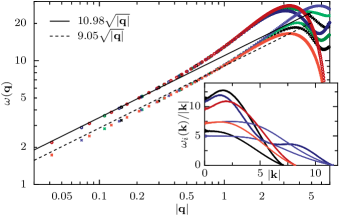
Figure 1: Inset: Full, three-dimensional dispersion curves $\omega_{i}/k$ used to extract the three elastic constants of a cubic crystal. We plot the longitudinal and transverse modes in the directions $(1,0,0)$ (red), $(1,1,0)$ (blue) and $(1,1,1)$ (black). The upper curves are longitudinal. For the orientations $(1,0,0)$ and $(1,1,1)$ the transverse modes are degenerate. Main curves: Dispersion relations in the confocal cut evaluated for the directions $(1,0)$, $(2,1)$, $(3,1)$, $(4,1)$ with respect to the hexagonal Bravais lattice. The lines are the analytic prediction for the long-wavelength limit, Eqs. (14) and (11). $58,000$ hours of computer time.

To better understand the limits of our theoretical calculation we performed a molecular dynamics simulation with $N=4,147,200$ particles organized in a face-centred cubic crystal, with a volume fraction $\phi=0.57$. We used event driven methods [20] because of their efficiency and also their long-time stability. The periodic simulation box contained $N_{1}\times N_{2}\times N_{3}=160\times 160\times 162$ particles and had a skew shape, aligned with the Bravais lattice. This choice allows easy data analysis since the simulation box is also aligned with the slice direction $(1,1,1)$, and it avoids ambiguities in the definition of the reciprocal vectors ${\mathbf{k}}$.

In order to study the mode structure of fluctuations we calculated and recorded the time average $\langle\hat{u}_{i}({\mathbf{k}})\hat{u}_{j}(-{\mathbf{k}})\rangle$ in three dimensions and deduced the polarization eigenstates by diagonalizing the three dimensional matrix of correlations measured for each ${\mathbf{k}}$. For the three-dimensional modes we find the expected scaling $d_{i}({\bf k})\sim k^{2}$ so that $\omega_{i}\sim k$. Thus when we plot $\omega_{i}/k$ as a function of $k$ (inset of Fig. 1) we can relate the small wavevector intersect to the three-dimensional isothermal elastic constants in Eq.(1). The transverse and longitudinal dispersion curves are then uniquely identified by their degeneracy, and they contain sufficient information to extract the three independent elastic constants of a cubic crystal [21]. We find the numerical values $\lambda,\mu,\nu=42.8,51.8,-53.8$ Units are chosen such that diameter, mass of all particles, and $kT$ are unity.

We now repeat the analysis for the sliced fluctuations of the crystal, $\langle\hat{u}_{\alpha}(-{\mathbf{q}})\hat{u}_{\beta}({\mathbf{q}})\rangle$, using the hexagonal $(1,1,1)$ planes to reproduce the experimental situation of [10, 7, 22], and extract the corresponding eigenvalues and auxiliary variables, $\omega_{i}({\bf q})$, from the resulting $2\times 2$ matrices. The result is plotted in the main figure of Fig. 1. We see that two branches are important at long wavelengths, and that as predicted in our analytic theory the dispersion relation for the modes are of the form $\omega^{2}_{i}({\mathbf{q}})\sim q$. Anomalous projected dispersion curves have already been observed experimentally in both disordered and crystalline materials [10, 22]. Using the effective elastic constants of Eqs. (11) together with the dispersion law eq. (14), we calculate the prefactors to this law and plot the results as the lines in Figure 1. The theoretical and measured curves agree to within $3\%$. We interpret these discrepancies as being due to the anisotropy of the crystal. We note that a face-centred cubic crystal with nearest-neighbour interactions is predicted in linear elasticity to have $\lambda/\mu=1$ and $\nu/\mu=-1$, see Eq. (12.7) of [23]. Our simulations find $\lambda/\mu=1.21$ and $\nu/\mu=-1.26$.

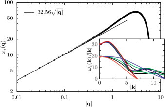
Figure 2: Inset: full dispersion curves for a two-dimensional hexagonal system. The upper curves are longitudinal, the lower ones are transverse; directions: red $(1,0)$, blue $(2,1)$, green $(3,1)$, black $(4,1)$. Main plot: Effective dispersion relation of a one-dimensional slice in the $(1,0)$ direction, compared to the theoretical prediction (solid line). Simulation of $400\times 400$ particles, $\phi=0.85$.

The use of the Fedorov form for the effective elastic constants is an uncontrolled approximation. To see to what degree the difference between theory and simulation is due to this approximation we also performed calculations and simulations of a two-dimensional ensemble of disks assembled in a hexagonal lattice projected onto a line. Since the two-dimensional elastic theory is isotropic [14] one can perform the projection without Fedorov’s approximation within linear elasticity. We measure again the two-dimensional dispersion curves in the inset of Fig. 2, and find a similar effective theory with $\omega^{2}=4q\mu(\lambda+2\mu)/(\lambda+3\mu)$ for the projection, which is the longitudinal branch of Eq. (14). The theoretical value for the coefficient is again plotted as a line. We find that there is no visible difference between the theory and the simulations for the projected system.

To conclude, we have shown that if we wish to describe an elastic slice observed in a confocal microscope as an effective medium we must introduce an effective dispersion relation in $|{\mathbf{q}}|$ which is very different from that which occurs in a normal two-dimensional medium with local interactions. Indeed in real-space one is obliged to consider that the system has long-ranged effective interactions. These interactions allow one to avoid Peierls’ result implying that a two-dimensional system should not display long-ranged order, due to the long-wavelength divergence of the expression for the mean squared amplitude of positional fluctuations: $\langle u^{2}\rangle\sim\int 1/q^{2}\;d^{2}{\mathbf{q}}$. This logarithmically diverging result is replaced by a regular expression due to the change in the dispersion law.

We have shown that to good accuracy one is able to relate the three-dimensional elastic constants and two-dimensional elastic behaviour. Thus observations in two dimensions can be used to deduce estimates of the three-dimensional constants. It will be particularly interesting in the future to study how disorder and glassiness modify these effective properties [8]. It is interesting to note that such an energy function in $|{\mathbf{q}}|$ was found in [24] where the spreading of a droplet was expressed as the effective dynamics of a contact line. Again we are in the presence of a system projected to lower dimensions.

References

- [1] \NameCheng Z., Zhu J., Russel W. B. Chaikin P. M. \REVIEWPhys. Rev. Lett. 8520001460.
-
[2]
\NamePrasad V., Semwogerere D. Weeks E. R. \REVIEWJournal of Physics:
Condensed Matter 192007113102.
http://stacks.iop.org/0953-8984/19/i=11/a=113102 - [3] \NameZahn K., Wille A., Maret G., Sengupta S. Nielaba P. \REVIEWPhys. Rev. Lett. 902003155506.
-
[4]
\NameKeim P., Maret G., Herz U. von Grünberg H. H. \REVIEWPhys. Rev.
Lett. 922004215504.
http://prl.aps.org/abstract/PRL/v92/i21/e215504 - [5] \NameChen K., Ellenbroek W. G., Zhang Z., Chen D. T. N., Yunker P. J., Henkes S., Brito C., Dauchot O., van Saarloos W., Liu A. J. Yodh A. G. \REVIEWPhys. Rev. Lett. 1052010025501.
- [6] \NameReinke D., Stark H., von Grünberg H.-H., Schofield A. B., Maret G. Gasser U. \REVIEWPhys. Rev. Lett. 982007038301.
- [7] \NameGhosh A., Chikkadi V. K., Schall P., Kurchan J. Bonn D. \REVIEWPhys. Rev. Lett. 1042010248305.
-
[8]
\NameGhosh A., Mari R., Chikkadi V., Schall P., Kurchan J. Bonn D.
\REVIEWSoft Matter 620103082.
http://dx.doi.org/10.1039/c0sm00265h -
[9]
\NameGhosh A., Mari R., Chikkadi V. K., Schall P., Maggs A. C. Bonn D. \REVIEWPhysica A 39020113061.
http://www.sciencedirect.com/science/article/pii/S037843711100207X - [10] \NameKaya D., Green N. L., Maloney C. E. Islam M. F. \REVIEWScience 3292010656.
- [11] \NameGhosh A., Chikkadi V., Schall P. Bonn D. \REVIEWPhys. Rev. Lett. 1072011188303.
- [12] \NameChaikin P. M. Lubensky T. C. \BookPrinciples of condensed matter physics (Cambridge University Press, Cambridge) 1995 sec. 6.4.
- [13] \NamePeierls R. \BookSurprises in Theoretical Physics (Princeton University Press, Princeton, N.J.) 1979.
- [14] \NameLandau L. Lifshitz E. \BookTheory of Elasticity: Course of Theoretical Physics, volume 7, Ch. 1, Section 10. (Butterworth-Heinemann) 1984.
- [15] \NameWallace D. C. \BookThermoelastic theory of stressed crystals and higher-order elastic constants in \BookSolid State Physics. Advances in Research and Applications, edited by \NameEhrenreich H., Seitz F. Turnbull D. Vol. 25 (Academic Press, New York and London) 1970 pp. 301–404.
- [16] \NameMorawiec A. \REVIEWPhys. Stat. Sol (b) 1841994313.
- [17] \NameFedorov A. F. I. \BookTheory of Elastic Waves in Crystals (Plenum Press, New York) 1968.
- [18] \NameNorris A. N. \REVIEWJ. Acoust. Soc. Am. 11920062114.
-
[19]
\NameSchindler M. Maggs A. C. \REVIEWEPJ E 3420111.
http://dx.doi.org/10.1140/epje/i2011-11115-7 - [20] \NameRapaport D. C. \BookThe art of molecular dynamics simulation 2nd Edition (Cambridge Univ. Press) 2004.
- [21] \NamePronk S. Frenkel D. \REVIEWPhys. Rev. Lett. 902003255501.
- [22] \NameGhosh A. \BookThesis (University of Amsterdam) 2011.
- [23] \NameBorn M. Huang K. \BookDynamical Theory of Crystal Lattices (Oxford University Press, Oxford) 1988.
-
[24]
\NameJoanny J. F. de Gennes P. G. \REVIEWJ. Chem. Phys.
811984552.
http://link.aip.org/link/?JCP/81/552/1