N-mode coherence in collective neutrino oscillations

Abstract

We study two-flavor neutrino oscillations in a homogeneous and isotropic ensemble under the influence of neutrino-neutrino interactions. For any density there exist forms of collective oscillations that show self-maintained coherence. They can be classified by a number $N$ of linearly independent functions that describe all neutrino modes as linear superpositions. What is more, the dynamics is equivalent to another ensemble with the same effective density, consisting of $N$ modes with discrete energies $E_{i}$ with $i=1,\ldots,N$. We use this equivalence to derive the analytic solution for two-mode (bimodal) coherence, relevant for spectral-split formation in supernova neutrinos. In this post-publication version, Eqs. (B4) and (B5) corrected.

I Introduction

In the early universe and in collapsing stars, the density of neutrinos is so large that they produce significant refractive effects for each other. In a seminal paper [1], Pantaleone showed that this is not just a correction to the usual matter effect [2, 3, 4], but causes qualitatively new phenomena. They originate from flavor off-diagonal refraction caused by neutrino oscillations which therefore feed back on themselves. One consequence is self-induced flavor conversion even for a very small mixing angle, caused by an instability of the interacting ensemble. When the density decreases slowly, for example in a supernova as a function of radius, this instability leads to flavor swaps between neutrino spectra in sharp energy intervals, causing conspicuous “spectral splits.” The body of literature on collective oscillations has immensely grown, so we cite only some theoretical key papers [5, 6, 7, 8, 9, 10, 11, 12, 13, 14, 15, 16, 17, 18, 19, 20, 21, 22, 23, 24, 25, 26], whereas we refer to a recent review [27] for the torrent of activities in the area of supernova neutrinos.

One key feature of collective oscillations is that, given suitable initial conditions, the entire ensemble evolves in a highly correlated way (self-maintained coherence). We make this concept more precise, if only for the simplest case of a homogeneous and isotropic gas with two mixed flavors and ignoring ordinary matter. Moreover, we mostly consider fixed density, although we use motivations related to adiabatic changes of density.

In the absence of neutrino-neutrino interactions, every mode evolves independently of the others. The ensemble may be described by two-spinors in flavor space $\psi_{E}(t)$, occupation-number matrices $\varrho_{E}(t)$, or the corresponding polarization vectors ${\bf P}_{E}(t)$—effectively there are three important numbers for every mode: the amplitudes of the two flavor components and their relative phase. We always use polarization vectors and label the modes with their vacuum oscillation frequency $\omega=\Delta m^{2}/2E$, where negative $\omega$ denote antineutrinos. Vacuum oscillations are described by the polarization vector of a given mode precessing with frequency $\omega$ around a direction given by a unit vector ${\bf B}$, the mass direction in flavor space. If neutrinos begin in weak-interaction eigenstates, all ${\bf P}_{\omega}$ are initially tilted relative to ${\bf B}$ by twice the vacuum mixing angle (Fig. 1). Each ${\bf P}_{\omega}$ precesses with a different frequency and so eventually the modes distribute themselves uniformly on the precession cone centered on ${\bf B}$, approaching complete kinematical decoherence.

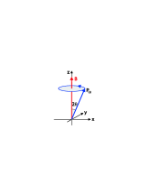
Figure 1: Precession of a polarization vector ${\bf P}_{\omega}$ with frequency $\omega$ around the $z$–direction (the mass direction in flavor space). The initial orientation is in the weak-interaction direction, tilted by twice the mixing angle relative to the $z$–direction.

Neutrino-neutrino interactions provide an additional force in terms of the global ${\bf P}=\int d\omega\,{\bf P}_{\omega}$, leading to the equations of motion (EoMs)

$$\dot{\bf P}_{\omega}=(\omega{\bf B}+\mu{\bf P})\times{\bf P}_{\omega}\,.$$ (1)

Here $\mu\sim\sqrt{2}\,G_{\rm F}n_{\nu}$ is a typical interaction energy, its exact value depending on the normalization of the polarization vectors. In the limit $\mu\to\infty$, and if initially all ${\bf P}_{\omega}$ are aligned in the flavor direction, they “stick together” and precess around ${\bf B}$ with the common frequency $\langle\omega\rangle$. These “synchronized oscillations” are the simplest case of self-maintained coherence [9, 11, 12].

Starting with such a configuration, $\mu$ can slowly decrease as in the expanding universe or with distance from a supernova. The ensemble continues to oscillate coherently, but the ${\bf P}_{\omega}$ slowly separate and fan out in a plane that precesses around ${\bf B}$. Such a pure precession mode can exist for any strength of $\mu$ [17, 22]. If $\mu$ decreases adiabatically to zero, the final configuration is that all ${\bf P}_{\omega}$ with $\omega$ above some frequency $\omega_{\rm split}$ point in the positive ${\bf B}$ direction, the others in the opposite direction, forming a “spectral split.”

More complicated forms of coherent motion occur in the context of multiple split formation [23]. A generic example is a gas of neutrinos and antineutrinos of a given flavor with a thermal distribution. Figure 2 shows a Fermi-Dirac distribution as a function of the re-scaled frequency $\omega=T/E$. In this way $\omega$ is a dimensionless variable of order unity. The neutrino flux streaming from a supernova core contains an excess of $\nu_{e}$ over $\bar{\nu}_{e}$ because the trapped electron-lepton number needs to be carried away. We mimic this situation schematically by assuming a small degeneracy parameter $\eta=0.2$, corresponding to $n_{\bar{\nu}}\approx 0.70\,n_{\nu}$. The region around $\omega=0$ corresponds to the high-$E$ tail and the high-$\omega$ tails (small $E$) fall off as $\omega^{-4}$. The mixing angle is taken to be very small and so the mass and flavor directions are almost identical. Notice that ${\bf P}_{\omega}$ pointing up means one flavor, pointing down the other. In the flavor-isospin convention [16, 23], the interpretation is reversed for antineutrinos, explaining that the spectrum in Fig. 2 is negative for $\omega<0$.

Figure 2: Neutrino spectrum ($z$-component of ${\bf P}_{\omega}$) in the variable $\omega=T/E$, assuming that initially only one flavor is populated with a Fermi-Dirac distribution (degeneracy parameter $\eta=0.2$). The integral over positive $\omega$ is normalized to unity.

Without $\nu$-$\nu$ interactions only small-amplitude vacuum oscillations occur, whereas for non-zero $\mu$ the system is unstable. The evolution is nicely illustrated by showing the instantaneous “swap factor” $z_{\omega}(t)$, i.e. the $\omega$-dependent factor by which the original spectrum must be multiplied to obtain the instantaneous $z$–component of ${\bf P}_{\omega}(t)$, i.e. $P_{\omega}^{z}(t)=z_{\omega}(t)P_{\omega}^{z}(0)$ [23] . The entire spectrum oscillates coherently. In the top panel of Fig. 3 we show numerical results ($\mu=10$) for the maximum and minimum $z_{\omega}$ during an oscillation period as well as their average.

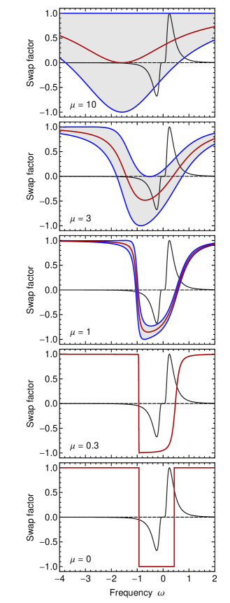
Figure 3: Maximum, minimum and average swap factor for the thermal spectrum of Fig. 2 if the interaction strength begins with $\mu=10$ and then decreases adiabatically to 0. Snapshots for $\mu=10$, 3, 1, 0.3 and 0 (top to bottom). The initial spectrum is overlaid using a vertically compressed scale relative to Fig. 2.

In this example and in any unstable spectrum, $z_{\omega}(t)$ is initially a Lorentzian of a certain width $\lambda$ that oscillates like an inverted gravitational pendulum with natural frequency equal to the same $\lambda$ [23]. When $\mu$ decreases adiabatically, $z_{\omega}$ changes, the oscillation amplitude decreases, and at $\mu=0$ takes on square-well shape: a spectral swap with two sharp splits at its edges has formed. Several snapshots are shown in Fig. 3.

These examples show “coherence” in some intuitive sense, but what precisely does this mean? We here define coherent motion as a form of evolution where neighboring modes do not separate from each other. Kinematical decoherence means that different ${\bf P}_{\omega}(t)$ within a frequency interval $\delta\omega$ eventually separate by a large amount, no matter how small $\delta\omega$. If we coarse-grain the ensemble with a bin width $\delta\omega$, the coarse-grained $\langle{\bf P}_{\omega}\rangle$ becomes shorter than ${\bf P}_{\omega}$ as time goes on [26]. On the other hand, coherence means that the coarse-grained ensemble remains identical with the original one, no matter how much time has passed. Pure precession is a trivial example because the polarization vectors remain static relative to each other, whereas in the example of Fig. 3, distant ${\bf P}_{\omega}(t)$ move wildly relative to each other, yet neighboring ones do not separate as time goes on.

Independent evolution of neighboring modes, no matter how close their frequencies, implies that every ${\bf P}_{\omega}(t)$ is linearly independent. For vacuum oscillations this is obvious because each ${\bf P}_{\omega}(t)$ is a harmonic function of frequency $\omega$. On the other hand, kinematical decoherence can not occur if every ${\bf P}_{\omega}(t)$ is a linear combination of a small number $N$ of independent functions. In this case the system performs what we call $N$-mode coherent oscillations. The infinitely dimensional function space required for kinematical decoherence has reduced to a small number of dimensions.

What is more, the same function space is spanned by the solutions ${\bf J}_{i}(t)$ of another system ($i=1,\ldots,N$) with vacuum frequencies $\omega_{i}$ and the same effective density. So we consider the EoMs of a new system

$$\dot{\bf J}_{i}=(\omega_{i}{\bf B}+\mu{\bf J})\times{\bf J}_{i}\,.$$ (2)

The functions ${\bf J}_{i}(t)$ can be found such that

$${\bf P}(t)={\bf J}(t)\,,$$ (3)

meaning that both systems are dynamically equivalent. The original modes ${\bf P}_{\omega}(t)$ and the linearly independent “carrier modes” ${\bf J}_{i}(t)$ span the same function space: each ${\bf P}_{\omega}(t)$ is a certain linear combination of the ${\bf J}_{i}(t)$. Notice that usually the carrier modes can not be interpreted as a coarse-grained representation of the original ensemble, but rather are more abstract.

The idea that coherence in collective neutrino oscillations corresponds to linear dependence among different modes and that the evolution is dynamically equivalent to a small ensemble of carrier modes provides a simple picture for self-maintained coherence. Our primary interest is to use this approach for the construction of explicit classes of solutions, notably for bimodal coherence.

We begin our study in Sec. II with the equations of motion, the idea of $N$-mode coherence, and the concept of carrier modes. Then we proceed to the explicit cases of single-mode, two-mode and multi-mode coherence in Secs. III–V and conclude in Sec. VI.

II N-Mode Coherence

II.1 Equations of motion

The two-flavor evolution of a homogeneous and isotropic neutrino gas can be described by flavor polarization vectors ${\bf P}_{\omega}(t)$, where $\omega=\Delta m^{2}/2E$ is the vacuum oscillation frequency. ${\bf P}_{\omega}$ pointing up means one flavor, pointing down the other. In the flavor-isospin convention [16], the interpretation is reversed for antineutrinos ($\omega<0$). The flavor evolution under the influence of vacuum oscillations and neutrino-neutrino interactions is given by Eq. (1). This precession equation has been stated many times [5, 6, 9, 11, 12, 18, 22, 27], most recently in great detail in Ref. [26], and we use it here without further ado.

A few points still deserve explicit mention. The polarization vectors derive from an ensemble average and thus are classical quantities. Our EoMs rely on a mean-field assumption: a given neutrino is supposed to feel only the average effect of all others, ignoring fluctuations or quantum correlations. (The quantum to classical transition was studied in Refs. [13, 14].) The length of ${\bf P}_{\omega}(t)$ is not fixed by a quantization condition, but chosen at convenience. The value of $\mu$ depends on this choice.

The EoMs conserve energy and derive from the classical Hamiltonian

$$H=\int\omega{\bf B}\cdot{\bf P}_{\omega}\,d\omega+\frac{\mu}{2}\,{\bf P}^{2}\,.$$ (4)

Here, $H$ and all ${\bf P}_{\omega}$ are functions of the canonical coordinates and momenta. The evolution of any function $F$ on phase space is given by the Poisson bracket $\dot{F}=[F,H]$. It is crucial that the ${\bf P}_{\omega}$ play the role of classical spins, or rather isospins. They obey the angular-momentum Poisson bracket $[P_{\omega,x},P_{\omega^{\prime},y}]=\delta(\omega-\omega^{\prime})\,P_{\omega,z}$ and cyclic permutations. Notice that $[\,{\cdot}\,,\,{\cdot}\,]$ is not a commutator—classical variables commute in the sense $P_{x}P_{y}=P_{y}P_{x}$. The overall ${\bf P}$ is the total angular momentum (in flavor space). Collective oscillations in the mean-field approximation are thus equivalent to a set of interacting classical spins. However, the simplicity of our Hamiltonian is deceiving because it encapsulates all the complications of collective flavor oscillations.

II.2 Rotating frames

Another conserved quantity is ${\bf P}$ projected on ${\bf B}$, equivalent to angular-momentum conservation in the symmetry direction. Therefore, we always work in the mass basis and use coordinates where the $z$–direction coincides with ${\bf B}$ (Fig. 1). Usually all ${\bf P}_{\omega}$ begin in a weak-interaction eigenstate and thus in a common direction that is tilted relative to ${\bf B}$ by twice the mixing angle.

The conservation of $P_{z}={\bf B}\cdot{\bf P}$ implies that the internal motion of the ensemble, up to overall precession, does not depend on $P_{z}$. Depending on convenience, we can study our system from the perspective of a frame co-rotating with some frequency [15]. We may choose $\omega_{\rm c}=\mu P_{z}$ and without loss of generality study the equivalent EoMs

$$\dot{\bf P}_{\omega}=(\omega{\bf B}+\mu{\bf P}_{\perp})\times{\bf P}_{\omega}\,,$$ (5)

where ${\bf P}_{\perp}$ is the part of ${\bf P}$ transverse to ${\bf B}$. We will frequently encounter the degeneracy between a shift of the neutrino $\omega$ spectrum by some amount $\omega_{\rm c}$ and $\mu P_{z}$. On the Hamiltonian level, such shifts amount to subtracting the conserved quantity $\omega_{\rm c}{\bf B}\cdot{\bf P}$.

Shifting a spectrum such as Fig. 2 by an amount $\omega_{\rm c}$ modifies the interpretation because negative-frequency modes (anti-neutrinos) become positive-frequency modes or vice versa. A mode that used to be occupied by $\bar{\nu}_{e}$ is then interpreted as being occupied, for example, by $\nu_{\mu}$. However, this modified interpretation does not affect the abstract dynamics, and we can always shift back at the very end. The possibility to shift anti-neutrino and neutrino modes seamlessly into each other is the main advantage of the flavor isospin convention.

II.3 Linear dependence of different modes

Collective neutrino oscillations consist of strong correlations among all modes and we have advanced that this means that the ${\bf P}_{\omega}(t)$ depend linearly on a small number $N$ of independent functions. To be more precise, we use $N$ to denote the number of nontrivial functions because in addition the constant ${\bf B}$ will be seen to appear, so ${\bf P}_{\omega}(t)$ actually depends on $N+1$ functions.

It is illuminating to diagnose $N$ in numerical examples. The ensemble is represented by a large discrete set ${\bf P}_{i}(t)$ with $i=1,\ldots,n$ and $n\gg 1$. To find the number of linearly independent functions on a time interval $t_{1}<t<t_{2}$ we calculate the Gram matrix $G_{ij}=\int_{t_{1}}^{t_{2}}dt\,{\bf P}_{i}(t)\cdot{\bf P}_{j}(t)$. Its rank reveals the number of linearly independent functions. In reality, one finds $N+1$ large eigenvalues of $G_{ij}$ and the rest very much smaller. They can be made ever smaller by increasing the degree of adiabaticity, i.e. slowing down $\mu(t)$ and decreasing the mixing angle, i.e. making the initial polarization vectors more collinear with ${\bf B}$. Within constraints of numerical accuracy, the chosen time interval is irrelevant to find $N+1$ if the ${\bf P}_{i}(t)$ are analytic functions, but of course influences the numerical realization of the Gram matrix.

We have always found the expected $N$. The formation of a single spectral swap as in Fig. 3 corresponds to bimodal coherence at any stage, i.e. the Gram matrix was found to have rank 3. The evolution from a double-crossed spectrum towards two swaps [23] corresponds to four-mode coherence (rank 5), and so forth.

II.4 Carrier modes

If every ${\bf P}_{\omega}(t)$ is a linear combination of $N$ independent functions and the constant ${\bf B}$ we may choose any set ${\bf P}_{\omega_{i}}(t)$ with $i=1,\ldots,N$ as a basis if they are not accidentally degenerate. We then have ${\bf P}(t)=\int d\omega\,{\bf P}_{\omega}(t)=a_{0}{\bf B}+\sum_{i=1}^{N}\,a_{i}{\bf P}_{\omega_{i}}(t)$ as a unique linear combination. We define ${\bf J}_{i}(t)\equiv a_{i}{\bf P}_{\omega_{i}}(t)$, obeying $\dot{\bf J}_{i}=(\omega_{i}{\bf B}+a_{0}\mu{\bf B}+\mu{\bf J})\times{\bf J}_{i}$ where ${\bf J}=\sum_{i=1}^{N}{\bf J}_{i}$. In a rotating frame we can transform away $a_{0}\mu{\bf B}$, or rather, we may choose another set ${\bf P}_{\omega_{i}^{\prime}}(t)$ where $a_{0}^{\prime}=0$.

So we can always find a set of linearly independent functions ${\bf J}_{i}(t)$ with $i=1,\ldots,N$ that obey Eq. (2), fulfill the matching condition Eq. (3), and together with ${\bf B}$ span the same function space as the original ensemble ${\bf P}_{\omega}(t)$. The internal dynamics of our system is the same if we study the co-rotating EoMs of Eq. (5). In this case the matching condition is ${\bf P}_{\perp}(t)={\bf J}_{\perp}(t)$ and the complication about the $a_{0}$ coefficient disappears.

We can express each ${\bf P}_{\omega}(t)$ of the original ensemble as a linear combination of the chosen “carrier modes” ${\bf J}_{i}(t)$

$${\bf P}_{\omega}(t)=b_{0}{\bf B}+\sum_{i=1}^{N}b_{i}\,{\bf J}_{i}(t)\,.$$ (6)

This function must obey the original EoM of Eq. (1). Inserting Eq. (6) on the l.h.s. of Eq. (1) and using Eq. (2) yields $\sum_{i=1}^{N}b_{i}(\omega_{i}{\bf B}+\mu{\bf J})\times{\bf J_{i}}$. On the r.h.s. of Eq. (1) we use ${\bf P}={\bf J}$ and Eq. (6) such that $-b_{0}\mu{\bf B}\times\mu{\bf J}+(\omega{\bf B}+\mu{\bf J})\times\sum_{i=1}^{N}b_{i}{\bf J}_{i}$. With ${\bf J}=\sum_{i=1}^{N}{\bf J}_{i}$ in the first term and after collecting everything we find

$$0={\bf B}\times\sum_{i=1}^{N}\bigl{[}b_{i}\,(\omega-\omega_{i})-b_{0}\mu\bigr{]}{\bf J}_{i}(t)\,.$$ (7)

The functions ${\bf J}_{i}(t)$ are linearly independent by construction and not proportional to ${\bf B}$. Therefore, we find the coefficient $b_{i}=b_{0}\mu/(\omega-\omega_{i})$ and thus

$${\bf P}_{\omega}(t)=b_{0}\left[{\bf B}+\sum_{i=1}^{N}\frac{\mu}{\omega-\omega_{i}}\,{\bf J}_{i}(t)\right]\,.$$ (8)

The required linear combination is unique up to an overall proportionality factor. (This linear combination is an example of a more general transformation briefly discussed in Appendix C.)

The expression, Eq. (8), is singular at the carrier frequencies. However, it is only the direction that matters, so we introduce the transformed carrier spectrum

$$\bar{\bf J}_{\omega}(t)=\left[{\bf B}+\sum_{i=1}^{N}\frac{\mu}{\omega-\omega_{i}}\,{\bf J}_{i}(t)\right]\prod_{i=1}^{N}\,(\omega-\omega_{i})\,,$$ (9)

where the overbar has nothing to do with antiparticles. Introducing the spectrum $g_{\omega}$ with $|{\bf P}_{\omega}|=|g_{\omega}|$, the original ensemble in terms of the carrier modes is

$${\bf P}_{\omega}=g_{\omega}\,\frac{\bar{\bf J}_{\omega}}{\bar{J}_{\omega}}\,,$$ (10)

where $\bar{J}_{\omega}=|\bar{\bf J}_{\omega}|$.

We usually consider initial conditions such that the ${\bf P}_{\omega}$ are almost collinear with ${\bf B}$ and we ask for the probability for a neutrino mode $\omega$ to stay in its original flavor, perhaps after an adiabatic change of $\mu$. This information is contained in the $z$–component of $\bar{\bf J}_{\omega}$ and we call

$$z_{\omega}(t)=\frac{{\bf B}\cdot\bar{\bf J}_{\omega}(t)}{\bar{J}_{\omega}}$$ (11)

the time-dependent “swap factor.”

Our discussion is motivated by the spectral swaps and splits that form when the effective density encoded in $\mu$ slowly decreases to zero. Since we are dealing with a Hamiltonian system, we expect the adiabatic change of the parameter $\mu$ to deform the solution, but that it remains coherent if it was initially coherent. For $\mu\to 0$ we have $\bar{\bf J}_{\omega}\propto{\bf B}$, implying that in the end all polarization vectors are collinear with ${\bf B}$. Conceivably one could define $N$-mode coherence by the very property of developing $N$ spectral splits when $\mu$ decreases adiabatically to zero.

Our main interest is to use these ideas to construct explicit classes of $N$-mode coherent solutions, notably the most general bimodal solution. For a set of functions ${\bf J}_{i}(t)$ fulfilling Eq. (2), the matching condition Eq. (3) is

$${\bf J}(t)=\int d\omega\,g_{\omega}\,\frac{\bar{\bf J}_{\omega}}{\bar{J}_{\omega}}\,.$$ (12)

For a given spectrum $g_{\omega}$ and interaction strength $\mu$ this condition restricts possible sets of carrier modes to provide an $N$-mode coherent solution.

III Single-Mode Coherence

A first trivial case is what we may call zero-mode coherence, where all ${\bf P}_{\omega}$ are exactly aligned with ${\bf B}$ and therefore stay that way. This configuration also appears as a limiting case of other forms of oscillation.

The first non-trivial case is single-mode coherence, identical with pure precession [17, 22]. The single carrier mode ${\bf J}(t)$ precesses around ${\bf B}$ with some co-rotation frequency $\omega_{\rm c}$ and obeys $\dot{\bf J}=\omega_{\rm c}{\bf B}\times{\bf J}$ where the nonlinear term $\mu{\bf J}\times{\bf J}=0$ has dropped out. According to Eq. (9) the transformed spectrum is $\bar{\bf J}_{\omega}=(\omega-\omega_{\rm c})\,{\bf B}+\mu{\bf J}$. The matching condition ${\bf P}={\bf J}$ then implies

$$\bar{\bf J}_{\omega}=(\omega-\omega_{\rm c})\,{\bf B}+\mu{\bf P}$$ (13)

and thus $\bar{\bf J}^{2}=(\omega-\omega_{\rm c}+\mu P_{z})^{2}+(\mu P_{\perp})^{2}$, where ${\bf P}_{\perp}$ denotes the part of ${\bf P}$ transverse to ${\bf B}$. The matching condition Eq. (12) is, in agreement with Ref. [22],

$$P_{z} = \int d\omega\,g_{\omega}\,\frac{\omega-\omega_{\rm c}+\mu P_{z}}{\sqrt{(\omega-\omega_{\rm c}+\mu P_{z})^{2}+(\mu P_{\perp})^{2}}}\,,$$

$$P_{\perp} = \int d\omega\,g_{\omega}\,\frac{\mu P_{\perp}}{\sqrt{(\omega-\omega_{\rm c}+\mu P_{z})^{2}+(\mu P_{\perp})^{2}}}\,.$$ (14)

We have used the fact that all ${\bf P}_{\omega}$ lie in the plane spanned by ${\bf B}$ and ${\bf P}$.

We could have studied our system from the perspective of a rotating frame as discussed in Sec. II.2. In the above expressions we recognize that nothing changes if we absorb $\mu P_{z}$ in the definition of $\omega_{\rm c}$.

For a given spectrum $g_{\omega}$ we can use these equations in different ways. If $P_{z}$ is fixed by an initial condition we may ask for the value of $P_{\perp}$ and $\omega_{\rm c}$ corresponding to a specified value of $\mu$. In particular, for $\mu\to 0$ we can find the split frequency for a given $P_{z}$. For explicit solutions in this sense and further discussions we refer to the literature [17, 22].

We may also use these conditions to construct all possible pure precession solutions for a given $g_{\omega}$. To this end we introduce the parameters $\kappa=\mu P_{\perp}$ and $\gamma=\omega_{\rm c}-\mu P_{z}$, leading to the general pure precession solution in the form of a two-parameter family depending on $\gamma$ and $\kappa$,

$$P_{\omega,z} = g_{\omega}\,\frac{\omega-\gamma}{\sqrt{(\omega-\gamma)^{2}+\kappa^{2}}}\,,$$

$$P_{\omega,\perp} = g_{\omega}\,\frac{\kappa}{\sqrt{(\omega-\gamma)^{2}+\kappa^{2}}}\,.$$ (15)

In addition one needs to specify the precession phase and thus the instantaneous orientation of the comoving plane. Integrating over $d\omega$ yields $P_{z}$ and $P_{\perp}$ and the corresponding $\mu=\kappa/P_{\perp}$ and $\omega_{\rm c}=\gamma+\mu P_{z}$.

In terms of the parameters $\kappa$ and $\gamma$, the swap factor for pure precession is

$$z_{\omega}=\frac{\omega-\gamma}{\sqrt{(\omega-\gamma)^{2}+\kappa^{2}}}\,.$$ (16)

Some examples are shown in Fig. 4. The step occurs at frequency $\gamma$ and the transition region has width $\kappa$.

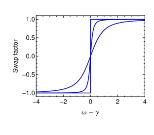
Figure 4: Swap factor for pure precession with $\kappa=0$, 0.5 and 1 according to Eq. (16).

For $\kappa\to 0$ the swap factor is identical with the sign function $z_{\omega}={\rm sgn}(\omega-\gamma)$. In this case the first relation in Eq. (III) has the form $P_{z}=\int d\omega\,g_{\omega}\,{\rm sgn}(\omega-\gamma)$ and can be used to find $\gamma$ for a given $P_{z}$. The second equation is $1=\int d\omega\,g_{\omega+\gamma}\,\mu/\sqrt{\omega^{2}+\kappa^{2}}$ and can be used to find $\kappa$ explicitly in the limit where $\mu$ is very small. In this limit, the integral is peaked around $\omega=0$ and we can approximately pull out $g_{\gamma}$. The remaining integral diverges for $\omega\to\pm\infty$, so we cut it off at some frequencies $\pm\alpha$, leading to $1\sim 2\mu g_{\gamma}\log(2\alpha/\kappa)$ and implying that for small $\mu$

$$\kappa\propto e^{-1/(2\mu g_{\gamma})}\,.$$ (17)

In other words, $\kappa$ becomes exponentially small for small $\mu$ or small $g_{\gamma}$.

IV Bimodal Coherence

IV.1 Matching conditions

Turning to bimodal coherence, we consider two carrier modes ${\bf J}_{1,2}(t)$ with frequencies $\omega_{1,2}$ fulfilling the precession equation, Eq. (2). According to Eq. (9) the transformed carrier spectrum is

$$\bar{\bf J}_{\omega} = (\omega-\omega_{1})(\omega-\omega_{2})\,{\bf B}$$ (18)

$${}+\mu\,(\omega-\omega_{2})\,{\bf J}_{1}+\mu\,(\omega-\omega_{1})\,{\bf J}_{2}\,.$$

Two interacting polarization vectors are dynamically equivalent to a gyroscopic pendulum (Appendix A). To use this equivalence we write $\omega_{1}=\omega_{\rm c}-\beta$ and $\omega_{2}=\omega_{\rm c}+\beta$, where $\omega_{\rm c}$ is a suitable co-rotation frequency such that the two carrier modes have equal but opposite frequencies $\pm\beta$. To simplify notation we implement $\omega_{\rm c}$ by shifting the spectrum, i.e. instead of $g_{\omega}$ we use $g_{\omega+\omega_{\rm c}}$ in the integral for the matching conditions.

From Appendix A we borrow ${\bf Q}={\bf J}_{1}-{\bf J}_{2}+(\beta/\mu)\,{\bf B}$ for the pendulum’s radius vector and find

$$\bar{\bf J}_{\omega}=\omega^{2}\,{\bf B}+\mu\,\omega\,{\bf J}+\mu\,\beta\,{\bf Q}\,,$$ (19)

where ${\bf J}={\bf J}_{1}+{\bf J}_{2}$ is the total angular momentum. To spell out the matching conditions we need a unit vector in the $\bar{\bf J}_{\omega}$ direction and thus need

$$\bar{\bf J}_{\omega}^{2} = \omega^{4}+(\mu\beta{\bf Q})^{2}+2\mu\omega^{2}(\beta{\bf B}\cdot{\bf Q}+{\textstyle\frac{1}{2}}\,\mu{\bf J}^{2})$$ (20)

$${}+2\mu\omega^{3}{\bf B}\cdot{\bf J}+2\mu^{2}\beta\omega\,{\bf Q}\cdot{\bf J}\,.$$

From Eq. (44) we take the natural frequency $\lambda^{2}=\beta\mu|{\bf Q}|$, so the second term is $\lambda^{4}$. The bracket in the third term is the energy $E$ of the pendulum. In the first term on the second line we have ${\bf B}\cdot{\bf J}=J_{z}$, a conserved quantity, and in the final term ${\bf Q}\cdot{\bf J}=|{\bf Q}|\,S$ with $S$ the spin (conserved angular momentum projection on the pendulum axis). Ordering by powers of $\omega$ we find

$$\bar{\bf J}_{\omega}^{2}=\omega^{4}+2\mu\,(\omega^{3}J_{z}+\omega^{2}E+\omega\lambda^{2}S)+\lambda^{4}\,.$$ (21)

As expected, this quantity is conserved, i.e. it does not depend on the oscillation phase.

We also need the individual components of $\bar{\bf J}_{\omega}$. We select directions in the plane transverse to ${\bf B}$ that move with the system and we call the direction along ${\bf J}_{\perp}$ the comoving $y$–direction, where ${\bf J}_{\perp}$ is the part of ${\bf J}$ transverse to ${\bf B}$. The comoving $x$–direction is then orthogonal and hence collinear with ${\bf B}\times{\bf J}$. We project out the three components by taking the scalar product of $\bar{\bf J}_{\omega}$ with ${\bf B}\times{\bf J}$, ${\bf J}_{\perp}={\bf J}-J_{z}{\bf B}$ and ${\bf B}$ and find

$$\bar{J}_{\omega,x} = \frac{\mu\beta\,{\bf Q}\cdot({\bf B}\times{\bf J})}{J_{\perp}}\,,$$

$$\bar{J}_{\omega,y} = \frac{\mu\omega\,{\bf J}_{\perp}^{2}+\mu\beta\,{\bf Q}\cdot{\bf J}_{\perp}}{J_{\perp}}\,,$$

$$\bar{J}_{\omega,z} = \omega^{2}+\mu\omega J_{z}+\mu\beta\,{\bf Q}\cdot{\bf B}\,.$$ (22)

On the l.h.s. of the matching condition Eq. (12) we have in these comoving coordinates ${\bf J}=(0,J_{\perp},J_{z})$ so that

$$\begin{pmatrix}0\\ 1\\ 0\end{pmatrix}=\int d\omega\,\frac{g_{\omega+\omega_{\rm c}}}{\bar{J}_{\omega}}\,\begin{pmatrix}1\\ \mu\omega\\ \omega^{2}\end{pmatrix}\,.$$ (23)

In the first line we have divided out $\bar{J}_{\omega,x}$ because it does not depend on $\omega$, and using this condition then simplifies the second line, and both are used to find the third. So we could find the matching conditions without even spelling out the scalar products in Eq. (IV.1).

Every solution is given in terms of the four pendulum parameters $E$, $S$, $J_{z}$ and $\lambda$, although we have not spelled out Eq. (IV.1) in terms of these conserved quantities. In addition we have the shift frequency $\omega_{\rm c}$ as a fifth parameter. However, we will see that $\omega_{\rm c}$ and $\mu J_{z}$ appear only combined, similar to the pure precession case, so actually there are only four independent parameters. The dynamics is given in terms of $\cos\theta$, the angle between ${\bf B}$ and ${\bf Q}$, that follows the pendulum differential equation of Eq. (49). In addition we can calculate the precession motion following the usual pendulum treatment (Appendix B).

Given the pendulum parameters and the EoM for $\cos\theta$ we have all the information needed to describe the motion. However, these parameters do not allow us to determine the original carrier modes in a unique way—there are many solutions. Notice, in particular, that the frequency $\beta$ and the length of ${\bf Q}$ are degenerate parameters. Two interacting polarization vectors are equivalent to a pendulum in flavor space, but the reverse mapping is not unique. In particular, the carrier frequencies are not unique. In certain limits, however, a particular choice may be most convenient.

IV.2 Swap parameters

While the pendulum parameters are well matched to the underlying dynamics, they are not very intuitive when studying cases such as the one shown in Fig. 3. To find a more suitable parametrization we first spell out the swap factor $z_{\omega}(t)=\bar{J}_{\omega,z}/\bar{J}_{\omega}$ explicitly,

$$z_{\omega}(t)=\frac{\omega^{2}+\mu\omega J_{z}+\lambda^{2}\cos\theta(t)}{\sqrt{\omega^{4}+2\mu\,(\omega^{3}J_{z}+\omega^{2}E+\omega\lambda^{2}S)+\lambda^{4}}}\,.$$ (24)

Inspecting the numerical results of Fig. 3, the analytic swap factor for pure precession of Eq. (16) motivates the following ansatz for the average swap factor

$$\bar{z}_{\omega}=\frac{(\omega-\gamma_{1})}{\sqrt{(\omega-\gamma_{1})^{2}+\kappa_{1}^{2}}}\frac{(\omega-\gamma_{2})}{\sqrt{(\omega-\gamma_{2})^{2}+\kappa_{2}^{2}}}\,,$$ (25)

where $\gamma_{1,2}$ give the location of the two steps and $\kappa_{1,2}$ their respective widths.

Comparing the coefficients of the $\omega$ polynomial in the denominators of Eqs. (24) and (25) provides

$$\lambda^{4} = (\gamma_{1}^{2}+\kappa_{1}^{2})(\gamma_{2}^{2}+\kappa_{2}^{2})\,,$$

$$\mu J_{z} = -(\gamma_{1}+\gamma_{2})\,,$$

$$\mu E = \frac{(\gamma_{1}+\gamma_{2})^{2}+2\gamma_{1}\gamma_{2}+\kappa_{1}^{2}+\kappa_{2}^{2}}{2}\,,$$

$$\mu S = -\frac{\gamma_{1}(\gamma_{2}^{2}+\kappa_{2}^{2})+\gamma_{2}(\gamma_{1}^{2}+\kappa_{1}^{2})}{\lambda^{2}}\,.$$ (26)

A further simplification is achieved if we express the time variation of the swap factor in terms of a new dimensionless variable

$$u(t)=\frac{\lambda^{2}\,\cos\theta(t)-\gamma_{1}\gamma_{2}}{\kappa_{1}\kappa_{2}}\,,$$ (27)

implying

$$z_{\omega}(t)=\frac{(\omega-\gamma_{1})(\omega-\gamma_{2})+\kappa_{1}\kappa_{2}\,u(t)}{\sqrt{[(\omega-\gamma_{1})^{2}+\kappa_{1}^{2}][(\omega-\gamma_{2})^{2}+\kappa_{2}^{2}]}}\,.$$ (28)

Inserting $u(t)$ in the EoM for $\cos\theta(t)$ of Eq. (49) and using the parameter mapping of Eq. (IV.2) provides

$$\dot{u}^{2}=(1-u^{2})\left[(\gamma_{1}-\gamma_{2})^{2}+(\kappa_{1}-\kappa_{2})^{2}+2\kappa_{1}\kappa_{2}(1-u)\right]\,,$$ (29)

where the range of motion is $-1\leq u\leq+1$. Therefore, the average is $\bar{u}=0$ and the average swap factor is indeed given by the proposed expression Eq. (25).

The structure of Eq. (29) suggests the interpretation $u=\cos\vartheta$ with $\vartheta(t)$ some abstract angle variable. In this way $1-u^{2}=\sin^{2}\vartheta$ and one finds

$$\dot{\vartheta}^{2}=(\gamma_{1}-\gamma_{2})^{2}+(\kappa_{1}-\kappa_{2})^{2}+2\kappa_{1}\kappa_{2}(1-\cos\vartheta)\,.$$ (30)

This angle always advances in the same direction with a modulated velocity. The EoM is that of a gravitational pendulum with a speed so large that it moves through the inverted position.

We show examples for the maximal, minimal and average swap factors, corresponding to $u=+1$, 0 and $-1$ in Fig. 5, where $\gamma_{1}=-1$, $\gamma_{2}=+1$ and $\kappa_{1}=0.1$ are held fixed and we show different cases for $\kappa_{2}=4$, 2, 1, 0.5 and 0.1 (top to bottom).

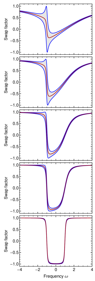
Figure 5: Maximum, minimum and average swap factor according to Eq. (28) using $\gamma_{1}=-1$, $\gamma_{2}=+1$, $\kappa_{1}=0.1$, and $\kappa_{2}=4$, 2, 1, 0.5 and 0.1 (top to bottom).

We realize that in Eqs. (28) and (29) the parameters $\gamma_{1}$ and $\gamma_{2}$ always appear either as $\gamma_{1}-\gamma_{2}$ or as $\omega-\gamma_{1,2}$. So we can go to a frame rotating with some frequency $\omega_{\rm c}$ by shifting $\omega$ and $\gamma_{1,2}$ by this amount and the solution will be the same. Since $-(\gamma_{1}+\gamma_{2})/\mu$ has the interpretation of $J_{z}$ this means that we can trade $J_{z}$ for a co-rotation frequency $\omega_{\rm c}$. Once more this is the same effect discussed in Sec. II.2. Instead of fixing $J_{z}=P_{z}$ it is enough to match ${\bf P}_{\perp}={\bf J}_{\perp}$ and trade the mismatch of $z$–components for a suitable co-rotation frequency $\omega_{\rm c}$. Here, in particular, we can adjust $J_{z}$ such that $\omega_{\rm c}=0$.

Spelling out the matching conditions in terms of the new parameters, we find

$$\begin{pmatrix}0\\ \mu^{-1}\\ P_{z}\end{pmatrix}=\int d\omega\,\frac{g_{\omega}}{\bar{J}_{\omega}}\,\begin{pmatrix}1\\ \omega\\ (\omega-\gamma_{1})(\omega-\gamma_{2})\end{pmatrix}\,,$$ (31)

where

$$\bar{J}_{\omega}=\sqrt{\left[(\omega-\gamma_{1})^{2}+\kappa_{1}^{2}\right]\left[(\omega-\gamma_{2})^{2}+\kappa_{2}^{2}\right]}\,.$$ (32)

For a given spectrum, the first equation establishes a constraint among the four parameters $\kappa_{1,2}$ and $\gamma_{1,2}$. The second allows us to calculate the required $\mu$ for this solution, and the third provides the required $P_{z}$. We can also use the first and second condition to simplify the third.

It is also of interest to spell out explicitly all three components of $\bar{\bf J}_{\omega}$ of Eq. (IV.1). For $J_{\perp}$ we find

$$(\mu{\bf J}_{\perp})^{2}=\kappa_{1}^{2}+\kappa_{2}^{2}-2\kappa_{1}\kappa_{2}u\equiv\kappa_{u}^{2}$$ (33)

and

$$\bar{J}_{\omega,x} = \frac{\sqrt{(\gamma_{2}-\gamma_{1})^{2}+\kappa_{u}^{2}}}{\kappa_{u}}\,\kappa_{1}\kappa_{2}\sqrt{1-u^{2}}\,,$$

$$\bar{J}_{\omega,y} = \frac{(2\omega-\gamma_{1}-\gamma_{2})\,\kappa_{u}^{2}+(\gamma_{2}-\gamma_{1})(\kappa_{2}^{2}-\kappa_{1}^{2})}{2\kappa_{u}}\,,$$

$$\bar{J}_{\omega,z} = (\omega-\gamma_{1})(\omega-\gamma_{2})+\kappa_{1}\kappa_{2}u\,.$$ (34)

Divide these components by $\bar{J}_{\omega}$ of Eq. (32) to find the unit vector $\bar{\bf J}_{\omega}/\bar{J}_{\omega}$.

For $-\infty<\omega<+\infty$ this vector traces a closed curve on the unit sphere, where the points $\omega=\pm\infty$ are at the north pole. This closed curve moves as a function of $\vartheta(t)$. Notice that for $u=\pm 1$, corresponding to the highest and lowest swap-factor curves in Fig. 3, the comoving $x$–component vanishes for all $\omega$, implying that all ${\bf P}_{\omega}$ lie in the plane spanned by ${\bf B}$ and ${\bf P}$. The case $u=-1$ corresponds to the lower swap factor, tracing out all $z$–values between $-1$ and $+1$, i.e. the unit vectors trace out the great circle spanned by ${\bf B}$ and ${\bf P}$.

IV.3 Pure precession limit: $\kappa_{1}\kappa_{2}=0$

Bimodal solutions are described by two carrier modes, which in turn are equivalent to a gyroscopic pendulum. One possible form of motion is pure precession: single-mode coherence appears as a limiting form of two-mode coherence. In terms of our swap parameters, this case is described by $\kappa_{1}=0$ or $\kappa_{2}=0$ where the solution is static up to an overall precession. The swap factor, no longer depending on time, is

$$z_{\omega}={\rm sgn}(\omega-\gamma_{1})\,\frac{(\omega-\gamma_{2})}{\sqrt{(\omega-\gamma_{2})^{2}+\kappa_{2}^{2}}}\,,$$ (35)

where we have used $\kappa_{1}=0$. In other words, we find the pure-precession swap factor of Eq. (16), augmented with a step function centered on a frequency $\gamma_{1}$ (Fig. 6). Therefore, our previous result is equal to the present one for the choice $\gamma_{1}\to-\infty$.

Figure 6: Swap factor for pure precession as derived from the gyroscopic pendulum picture. The chosen parameters are $\gamma_{1}=-1$, $\gamma_{2}=+1$, $\kappa_{1}=0$ and $\kappa_{2}=0.5$.

IV.4 Pure nutation limit: $\kappa_{1}=\kappa_{2}$

Another limiting case is when the swap factor is symmetric around $\omega_{\rm c}=\frac{1}{2}(\gamma_{1}+\gamma_{2})$, i.e. when $\kappa_{1}=\kappa_{2}\equiv\kappa$. In a frame co-rotating with $\omega_{\rm c}$ this solution is equivalent to a plane pendulum where $J_{z}=S=0$ and was found previously [23]. Shifting $\omega$ and $\gamma_{1,2}$ by $\omega_{\rm c}$ reproduces the pure nutation solution

$${\bf P}_{\omega+\omega_{\rm c}}=\frac{g_{\omega+\omega_{\rm c}}}{\sqrt{\omega^{4}+2\omega^{2}\lambda^{2}c_{\rm m}+\lambda^{4}}}\begin{pmatrix}\lambda^{2}s\cr\omega\lambda\sqrt{2(c_{\rm m}-c)}\cr\omega^{2}+\lambda^{2}c\cr\end{pmatrix}\,,$$ (36)

where $s=\sin\theta$, $c=\cos\theta$, and $c_{\rm m}=\cos\theta_{\rm min}$. In contrast with Ref. [23] we here count the zenith angle $\theta$ from the north pole. In the co-rotating frame we have $\gamma_{1,2}=\pm\gamma$ and therefore the natural pendulum frequency is $\lambda^{2}=\kappa^{2}+\gamma^{2}$, whereas the plane pendulum’s highest point is given by $c_{\rm m}=(\kappa^{2}-\gamma^{2})/(\kappa^{2}+\gamma^{2})$.

If the system has been set up with all polarization vectors initially almost aligned with ${\bf B}$, the initial swap factor is unity. The initial swap parameters are $\gamma_{1}=\gamma_{2}=\omega_{\rm c}$ and $\kappa_{1}=\kappa_{2}=\kappa$ and are solutions of [23]

$$0 = \int d\omega\,g_{\omega}\,\frac{1}{(\omega-\omega_{\rm c})^{2}+\kappa^{2}}\,,$$

$$\frac{1}{\mu} = \int d\omega\,g_{\omega}\,\frac{\omega-\omega_{\rm c}}{(\omega-\omega_{\rm c})^{2}+\kappa^{2}}\,.$$ (37)

For the example of Fig. 3 with the initial value $\mu=10$ one finds $\omega_{\rm c}=-1.604$ and $\kappa=2.179$.

IV.5 Two pure precessions: $\kappa_{1,2}\ll|\gamma_{2}-\gamma_{1}|$

When we begin with a bimodal system and the density decreases adiabatically to zero, the end state shows a spectral swap with two splits at its edges (Fig. 3). When $\mu$ has become sufficiently small, the two quasi-step functions are well separated and the overall swap factor looks like the product of two pure precessions. This observation was the very motivation for writing the general bimodal solution in terms of the swap parameters $\gamma_{1,2}$ and $\kappa_{1,2}$ instead of the pendulum parameters $\lambda$, $E$, $J_{z}$ and $S$.

In the present limit of $\kappa_{1,2}\ll|\gamma_{2}-\gamma_{1}|$, the two split regions are essentially independent. The carrier modes ${\bf J}_{1,2}(t)$ precess essentially freely with frequencies $\gamma_{1,2}$. To study this case it is easiest to represent the $x$–$y$–components of all polarization vectors as complex numbers of the form $J_{x}+{\rm i}J_{y}$, so the transverse components of the carrier modes can be chosen as $\kappa_{1}e^{{\rm i}\gamma_{1}t}$ and $\kappa_{2}e^{{\rm i}\gamma_{2}t}$ with $\kappa_{1}=\mu|{\bf J}_{1,\perp}|$ and $\kappa_{2}=\mu|{\bf J}_{2,\perp}|$. The abstract angle characterizing the overall motion is here $\vartheta=\pm(\gamma_{1}-\gamma_{2})t$ because in the present limit $\dot{\vartheta}^{2}=(\gamma_{1}-\gamma_{2})^{2}$.

In the lower panels of Fig. 3 we see that the swap factor is asymmetric and steeper in the region where the step falls into a spectral region where $g_{\omega}$ is smaller. This is explained by Eq. (17) where we have shown that for a pure precession with very small $\mu$ the width of the step is exponentially smaller for smaller $g_{\omega}$ in the step region.

As $\mu$ decreases adiabatically in a case like Fig. 3, the system begins in a state of pure nutation and ends in a state of two independent pure precessions. These limiting forms and all intermediate cases are described by our four-parameter analytic solution.

IV.6 Numerical examples

To test if our analytic solution indeed corresponds to numerical examples such as Fig. 3, we extract the parameters $\gamma_{1,2}$ and $\kappa_{1,2}$ as $\mu$ slowly decreases (Fig. 7). Comparing the analytic swap factor with the numerical one yields perfect agreement.

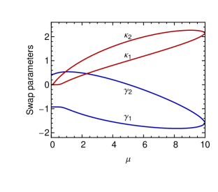
Figure 7: Numerically determined swap parameters $\gamma_{1,2}$ and $\kappa_{1,2}$ for the example of Fig. 3 as a function of $\mu$ that adiabatically decreases from 10 to 0.

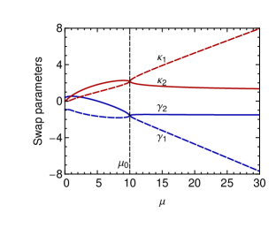
Figure 8: Same as Fig. 7, now with $\mu$ being decreased from $\mu_{0}=10$ to zero as before, or increased from $\mu_{0}=10$ to infinity.

Usually we begin with ${\bf P}_{\omega}^{0}$ almost aligned with ${\bf B}$ and a chosen $\mu_{0}$. Then $\mu$ decreases from $\mu_{0}$ to 0, going through different solutions as in Fig. 3 where $P_{z}$ remains conserved. If in this example we were to begin with $\mu_{0}=3$ instead of 10, the $\mu=3$ solution would be the one with a Lorentzian pattern. So for the same $g_{\omega}$, $P_{z}$ and $\mu$ there exist different solutions that we can construct numerically by adiabatic deformations.

We may also begin with a certain $\mu_{0}$ and then increase the density as during supernova collapse. The initial pure nutation is then deformed to another bimodal solution within our general four-parameter family. For our usual example of Fig. 3 we show the swap parameters as a function of $\mu$ in Fig. 8, assuming the initial value is $\mu_{0}=10$. The solutions for $0<\mu<\mu_{0}$ are from Fig. 7. We identify the parameters such that $\gamma_{1}<\gamma_{2}$.

V Multi-Mode Coherence

V.1 Four-mode coherence

More complicated forms of motion occur if the spectrum has two or more independent instabilities, typically for multi-crossed spectra [23]. Such spectra arise naturally if we augment the Fermi-Dirac spectrum of a single species (Fig. 2) with an initial population of the other species, but with a larger temperature and smaller flux. This mimics neutrinos streaming from a supernova core where a larger flux of $\nu_{e}$ than $\bar{\nu}_{e}$ stream away and the other flavors $\nu_{\mu}$ and $\nu_{\tau}$ have smaller fluxes, larger average energies, and no asymmetry. So if we add to the asymmetric spectrum of Fig. 2 a symmetric component of the other flavor with a 1.25 times larger $T$ and 0.8 times smaller number density, the difference spectrum relevant for flavor oscillations is shown in Fig. 9.

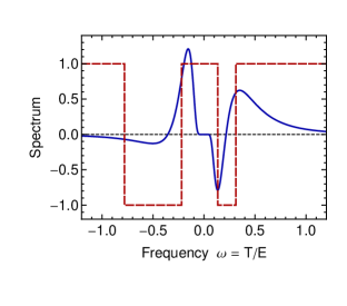
Figure 9: Difference spectrum between two flavors. One is a Fermi-Dirac distribution ($\eta=0.2$) as in Fig. 2, the other a nondegenerate spectrum with 1.25 larger $T$ and 0.8 times smaller $\nu$ density. The integral over positive $\omega$ of the degenerate flavor is normalized to unity. Overlaid is the final swap factor after $\mu$ has decreased adiabatically from 3 to 0.

This spectrum has two zero crossings with positive slope, allowing for two independent instabilities, i.e. Eq. (IV.4) can have two solutions [23]. If $\mu$ decreases adiabatically from some value $\mu_{0}$ to 0, one finds two spectral swaps and four concomitant splits. As an example we show the final swap factor for $\mu_{0}=3$ in Fig. 9.

This case is an example for four-mode coherence. The complicated motion of all ${\bf P}_{\omega}$ is equivalent to four carrier modes as confirmed by numerical tests using the Gram matrix. When $\mu$ has become very small and the swaps are almost complete, we have the now-familiar pattern of four independent pure precessions in the four split regions. In the final small-$\mu$ limit, the swap factor is

$$z_{\omega}=\prod_{i=1}^{4}\,\frac{\omega-\gamma_{i}}{\sqrt{(\omega-\gamma_{i})^{2}+\kappa_{i}^{2}}}\,,$$ (38)

corresponding to four freely precessing carrier modes.

Equation (9) implies that $\bar{\bf J}_{\omega}^{2}$ is now a polynomial with leading term $\omega^{8}$, so the above representation for $z_{\omega}$ is general, except that in the numerator complicated time-dependent terms appear when we are not in the small-$\mu$ limit. One can group the four carrier modes in pairs and understand the overall motion as two gyroscopic pendulums interacting by a dipole force. Apart from an overall precession, the time dependence is then described by two nutation angles and one relative precession angle.

If we choose some value for $\mu_{0}$, it is not assured that the system indeed has two instabilities—it can have only one or none. Therefore, as $\mu$ adiabatically decreases, the system can at first show bimodal coherence and at some critical $\mu$-value the second unstable mode kicks in, taking the system to a state of four-mode coherence.

V.2 Stability issues

It is generic that a system of lower modality can develop higher modality by an instability. Usually we begin with all polarization vectors almost aligned with ${\bf B}$. If they were perfectly aligned, we would have zero-mode coherence for any spectrum $g_{\omega}$, but the smallest disturbance allows the unstable modes to grow exponentially. We implement this disturbance in the form of a small mixing angle, i.e. a small mismatch between the initial condition and exact zero-mode coherence. The solutions ($\omega_{\rm c},\kappa$) of Eq. (IV.4) identify the unstable modes, each one corresponding to a contribution of 2 to the total modality $N$ relevant for the given $g_{\omega}$ and $\mu$.

We can also prepare a state of pure precession. With an arbitrary spectrum $g_{\omega}$ and parameters $\gamma$ and $\kappa$, the initial condition is defined by Eq. (III), allowing us to calculate the required $\mu$. Henceforth the system evolves in single-mode coherent motion unless it is unstable. Depending on $g_{\omega}$ and with the slightest disturbance it can transit, for example, to three-mode coherence. Likewise, we can set up the system in some state of bimodal coherence with suitably chosen parameters $\kappa_{1,2}$ and $\gamma_{1,2}$, yet it can transit to higher-mode coherence.

A formal stability criterion is only available for zero-mode coherence in the form of Eq. (IV.4) that allows us to decide, without solving the EoMs, if the system is stuck in its alignment with ${\bf B}$ or not.

VI Conclusions

We have studied two-flavor neutrino oscillations in a homogeneous and isotropic neutrino gas under the influence of neutrino-neutrino refraction. This system is equivalent to an ensemble of classical spins, each labeled by its vacuum precession frequency $\omega$ around an external magnetic field ${\bf B}$ and a dipole-dipole interaction with identical strength $\mu$ between any pair of spins.

We have argued that the conspicuous “self-maintained coherence” found in this system can be understood in terms of an equivalent “carrier system” of a few discrete modes with the same dynamics. We have provided an explicit construction of how the original system depends linearly on the carrier system, assuming certain matching conditions. We have used this approach to construct the most general bimodal solution.

Self-maintained coherence is to be contrasted with kinematical decoherence. We have only studied “purely coherent” forms of motion, but of course, depending on initial conditions, the system can partly or fully decohere. We have not pursued the fascinating question of order vs. disorder in our system [6, 26].

Our results pertain to the simplest possible toy model and as such do not have any immediate practical impact on issues of supernova neutrino oscillations. The next step should be to apply these ideas to more realistic situations, notably “multi-angle cases,” where isotropy is no longer assumed. The main unresolved issues in the theory of collective neutrino oscillations in the context of supernova neutrinos remains the role of multi-angle effects. Every neutrino mode depends on energy and on its direction of motion, introducing much greater complications. It would be surprising if it were not possible to develop a more analytical understanding of collective flavor oscillations than has been achieved by deconstructing numerical examples. We imagine that our results are only a first step toward a more complete theory of collective flavor oscillations. The ultimate goal is to provide a thorough theoretical underpinning for what one is observing in numerical simulations, and perhaps eventually in the neutrino signal of the next galactic supernova.

Note Added

As this paper went to press, a preprint appeared [28] that studies in detail the properties of the quantum version of our Hamiltonian, Eq. (4), and in particular its invariants. The constants of the motion discussed in our Appendix C are identified as the so-called Gaudin magnet Hamiltonians.

Appendix A Two polarization vectors

We briefly review the equivalence between the dynamics of two interacting polarization vectors with that of a gyroscopic pendulum [20]. Consider the classical Hamiltonian for two spin angular momenta ${\bf P}_{1}$ and ${\bf P}_{2}$ interacting with an external magnetic field and with each other by a dipole interaction of strength $\mu$,

$$H={\bf B}\cdot(\omega_{1}{\bf P}_{1}+\omega_{2}{\bf P}_{2})+\mu\,{\bf P}_{1}\cdot{\bf P}_{2}\,.$$ (39)

As usual, ${\bf B}$ is a unit vector in the $z$-direction and $\omega_{1,2}$ the precession frequencies in the absence of $\mu$. Each of ${\bf P}_{1,2}$ obeys Poisson brackets which for an angular momentum ${\bf L}$ are $[L_{i},L_{j}]=\epsilon_{ijk}L_{k}$. The Poisson brackets of the components of ${\bf P}_{1}$ with those of ${\bf P}_{2}$ vanish and thus ${\bf P}_{1,2}^{2}$ is conserved. Therefore, we may add $(\mu/2)\,({\bf P}_{1}^{2}+{\bf P}_{2}^{2})$ to the Hamiltonian and find

$$H={\bf B}\cdot(\omega_{1}{\bf P}_{1}+\omega_{2}{\bf P}_{2})+\frac{\mu}{2}\,{\bf P}^{2}\,,$$ (40)

where ${\bf P}={\bf P}_{1}+{\bf P}_{2}$ is the total angular momentum. The EoMs $\dot{\bf P}_{1,2}=[{\bf P}_{1,2},H]$ finally are

$$\dot{\bf P}_{1,2}=(\omega_{1,2}{\bf B}+\mu\,{\bf P})\times{\bf P}_{1,2}$$ (41)

and thus the usual precession equations.

To simplify the EoMs we introduce $\beta=\frac{1}{2}\,(\omega_{1}-\omega_{2})$ and $\omega_{\rm c}=\frac{1}{2}\,(\omega_{1}+\omega_{2})$, leading to $\dot{\bf P}_{1,2}=[(\omega_{\rm c}\pm\beta)\,{\bf B}+\mu\,{\bf P}]\times{\bf P}_{1,2}$. The only effect of $\omega_{\rm c}$ is a common rotation around ${\bf B}$. Therefore, we go to a rotating frame where $\omega_{\rm c}=0$ and thus effectively $\omega_{1,2}=\pm\beta$. Adding and subtracting these equations provides

$$\dot{\bf Q}=\mu\,{\bf P}\times{\bf Q}\quad\hbox{and}\quad\dot{\bf P}=\beta\,{\bf B}\times{\bf Q}\,,$$ (42)

where ${\bf Q}={\bf P}_{1}-{\bf P_{2}}-(\beta/\mu)\,{\bf B}$ has conserved length. Up to a constant, the Hamiltonian becomes

$$H=\beta\,{\bf B}\cdot{\bf Q}+\frac{\mu}{2}\,{\bf P}^{2}\,.$$ (43)

It is reminiscent of a gyroscopic pendulum with moment of inertia $I=\mu^{-1}$. The first term is the “gravitational potential” of the center of mass which is constrained to move on a sphere with radius $|{\bf Q}|$. The second is the kinetic energy of the total angular momentum ${\bf P}$.

However, the algebraic properties of ${\bf Q}$ change. Earlier its Poisson brackets derived from its constituent angular momenta. However, the radius-vector interpretation requires $[Q_{i},Q_{j}]=0$ and $[P_{i},Q_{j}]=\epsilon_{ijk}Q_{k}$, where $P_{i}$ are the components of ${\bf P}$. Remarkably, the EoMs of Eq. (42) also follow with the new Poisson brackets for ${\bf Q}$.

In both cases, the conserved quantities are $H$ (energy), ${\bf B}\cdot{\bf P}$ (angular momentum along the force direction), ${\bf Q}^{2}$ (length of the pendulum), and ${\bf Q}\cdot{\bf P}$ (total angular momentum projected on the radius vector or spin). The quantity $\lambda$ defined by

$$\lambda^{2}=\beta\mu\,|{\bf Q}|$$ (44)

plays the role of the natural pendulum frequency.

Appendix B Gyroscopic Pendulum

We briefly review the textbook treatment of the symmetric heavy top, also known as Lagrangian top, gyroscopic pendulum, or spherical pendulum with spin. It is an axially symmetric body, spinning around its symmetry axis (moment of inertia $I_{3}$) and supported on this axis. Its moment of inertia relative to the point of support is $I_{1}$, mass $M$, gravitational acceleration $g$ along the $z$–direction, distance $\ell$ between point of support and center of mass, and angle $\theta$ relative to the $z$–direction. Therefore, $V=Mg\,\ell\,\cos\theta$ is the potential energy.

The angular momentum ${\bf S}$ along the symmetry axis (spin) has kinetic energy $T_{\rm spin}={\bf S}^{2}/(2I_{3})=I_{3}\omega_{\rm spin}^{2}/2$. The point of support being on the symmetry axis prevents a torque to change $S=|{\bf S}|$ and so both $S$ and $\omega_{\rm spin}$ are conserved. The overall motion is independent of the internal spin angle and all tops with the same $S$ but different $I_{3}$ and $\omega_{\rm spin}$ move in the same way. Therefore, we may use a single moment of inertia $I\equiv I_{1}=I_{3}$ to describe the system.

The orbital angular momentum is ${\bf L}=I\,{\bf q}\times{\dot{\bf q}}$, where ${\bf q}$ is a unit vector along the symmetry axis. It marks the top’s orientation with zenith angle $\theta$ and azimuthal angle $\varphi$. The orbital kinetic energy is

$$T_{\rm orbital}=\frac{{\bf L}^{2}}{2I}=\frac{1}{2}\,I\,\dot{\bf q}^{2}=\frac{1}{2}\,I\,\bigl{(}\dot{\theta}^{2}+\dot{\varphi}^{2}\sin^{2}\theta\bigr{)}\,.$$ (45)

The total angular momentum ${\bf J}={\bf L}+{\bf S}$ has conserved $z$–component, where $S_{z}=S\,\cos\theta$ and $L_{z}=I\dot{\varphi}\sin^{2}\theta$. Here one factor of $\sin\theta$ comes from the projection of ${\bf q}$ on the transverse plane and the velocity is $\dot{\varphi}\sin\theta$. Therefore, $J_{z}=I\dot{\varphi}\sin^{2}\theta+S\cos\theta$ is conserved and

$$\dot{\varphi}=\frac{J_{z}-S\cos\theta}{I\sin^{2}\theta}\,.$$ (46)

Therefore

$$T_{\rm orbital}=\frac{1}{2}\,I\,\dot{\theta}^{2}+\frac{(J_{z}-S\cos\theta)^{2}}{2I\sin^{2}\theta}$$ (47)

and the total energy $E=T+V$ is

$$E=\frac{I}{2}\,\dot{\theta}^{2}+\frac{(J_{z}-S\cos\theta)^{2}}{2I\sin^{2}\theta}+Mg\ell\cos\theta\,.$$ (48)

This has the form $E=I\,\dot{\theta}^{2}/2+V(\theta)$, where $V(\theta)$ is a potential given in terms of conserved quantities fixed by initial conditions. One may now solve for $\theta(t)$ by a quadrature and then find $\varphi(t)$ by integrating Eq. (46).

Next we introduce $c=\cos\theta$ as independent variable so that $\dot{\theta}^{2}=\dot{c}^{2}/\sin^{2}\theta$ and find the usual third-order polynomial in $c$,

$$\dot{c}^{2}=2\,\frac{E-Mg\ell\,c}{I}\,(1-c^{2})-\frac{(J_{z}-S\,c)^{2}}{I^{2}}\,,$$ (49)

that can be integrated using elliptic functions. A typical motion is nutation between two limiting angles $\theta_{1}$ and $\theta_{2}$ as well as precession. When $J_{z}=S=0$ we have a plane pendulum where

$$\lambda^{2}=Mg\,\ell/I$$ (50)

gives us the natural frequency $\lambda$.

The motion of two interacting polarization vectors is equivalent to a gyroscopic pendulum (Appendix A) and therefore can be explicitly solved in terms of elliptic functions. This feat was achieved previously without invoking the equivalence to a pendulum [10].

Appendix C Transformed ensemble of polarization vectors

The functions $\bar{\bf J}_{\omega}(t)$ derived from the carrier modes by Eqs. (8) or (9) represent a special case of a more general transformation of an ensemble ${\bf P}_{\omega}(t)$ obeying Eq. (1). To motivate this transformation we observe that in the non-interacting case, every ${\bf B}\cdot{\bf P}_{\omega}$ is conserved. Is there a similar conserved quantity in the interacting case?

So we look for a vector ${\bf X}$ such that ${\bf X}\cdot{\bf P}_{\omega}$ is conserved. A trivial example is ${\bf X}={\bf P}_{\omega}$, but any other ${\bf X}$ fulfilling $\dot{\bf X}=(\omega{\bf B}+\mu{\bf P})\times{\bf X}$ is a solution. To see this consider $\dot{\bf X}(t)={\bf V}(t)\times{\bf X}(t)$, where ${\bf V}(t)$ is externally prescribed and solve for ${\bf X}(t)$ with initial condition ${\bf X}_{0}$. Another initial condition ${\bf Y}_{0}$ provides ${\bf Y}(t)$ and ${\bf X}(t)\cdot{\bf Y}(t)$ is conserved. Consider $d({\bf X}\cdot{\bf Y})/dt=\dot{\bf X}\cdot{\bf Y}+{\bf X}\cdot{\dot{\bf Y}}=({\bf V}\times{\bf X})\cdot{\bf Y}+{\bf X}\cdot({\bf V}\times{\bf Y})$ and after a permutation in one of the triple products one finds $d({\bf X}\cdot{\bf Y})/dt=0$.

We seek ${\bf X}$ as a linear combination of the ${\bf P}_{\omega}$ and also of ${\bf B}$ because ${\bf X}={\bf B}$ is a solution for $\mu\to 0$. The length of ${\bf X}$ is arbitrary, so we assume the form ${\bf X}={\bf B}+\int d\omega^{\prime}\,a_{\omega^{\prime}}{\bf P}_{\omega^{\prime}}$ and seek the coefficients $a_{\omega^{\prime}}$. The requirement $\dot{\bf X}=(\omega{\bf B}+\mu{\bf P})\times{\bf X}$ implies $\int d\omega^{\prime}\,a_{\omega^{\prime}}\dot{\bf P}_{\omega^{\prime}}=(\omega{\bf B}+\mu{\bf P})\times\left({\bf B}+\int d\omega^{\prime}\,a_{\omega^{\prime}}{\bf P}_{\omega^{\prime}}\right)$. On the l.h.s. we insert $\dot{\bf P}_{\omega^{\prime}}=(\omega^{\prime}{\bf B}+\mu{\bf P})\times{\bf P}_{\omega^{\prime}}$, whereas on the r.h.s. we use ${\bf B}\times{\bf P}={\bf B}\times\int d\omega^{\prime}{\bf P}_{\omega^{\prime}}$. Collecting all terms we find $0={\bf B}\times\int d\omega^{\prime}\,\left[(\omega-\omega^{\prime})a_{\omega^{\prime}}-\mu\right]\,{\bf P}_{\omega^{\prime}}$ and thus $a_{\omega^{\prime}}=\mu/(\omega-\omega^{\prime})$.

We are therefore led to define the linearly transformed polarization vectors

$${\bar{\bf P}}_{\omega}(t)={\bf B}+\mu\int d\omega^{\prime}\,\frac{{\bf P}_{\omega^{\prime}}(t)}{\omega-\omega^{\prime}}\,.$$ (51)

The integral is essentially the Hilbert transform in the $\omega$ variable and is understood as a Cauchy principal value. (The Hilbert transform of a function $f(x)$ is defined as its convolution with $1/x$.) So we have found a unique linear combination $\bar{\bf P}_{\omega}(t)$ of the original ensemble ${\bf P}_{\omega}(t)$ that obeys the original precession equation in the form

$$\partial_{t}{\bar{\bf P}}_{\omega}=(\omega{\bf B}+\mu{\bf P})\times\bar{\bf P}_{\omega}\,.$$ (52)

As a consequence, ${\bf P}_{\omega}^{2}$, $\bar{\bf P}_{\omega}^{2}$, and ${\bf P}_{\omega}\cdot\bar{\bf P}_{\omega}$ are conserved for any fixed $\mu$.

The intriguing properties of the transformed ensemble remain to be explored. We believe, for example, that coherent oscillations correspond to ${\bf P}_{\omega}(t)$ and $\bar{\bf P}_{\omega}(t)$ being collinear at all times.

References

- [1] J. Pantaleone, Phys. Lett. B 287, 128 (1992).
- [2] L. Wolfenstein, Phys. Rev. D 17, 2369 (1978).
- [3] S. P. Mikheev and A. Y. Smirnov, Sov. J. Nucl. Phys. 42, 913 (1985) [Yad. Fiz. 42, 1441 (1985)].
- [4] T. K. Kuo and J. T. Pantaleone, Rev. Mod. Phys. 61, 937 (1989).
- [5] G. Sigl and G. Raffelt, Nucl. Phys. B 406, 423 (1993).
- [6] J. Pantaleone, of oscillating neutrinos,” Phys. Rev. D 58, 073002 (1998).
- [7] S. Samuel, Phys. Rev. D 48, 1462 (1993).
- [8] V. A. Kostelecký and S. Samuel, Phys. Lett. B 318, 127 (1993).
- [9] V. A. Kostelecký and S. Samuel, Phys. Rev. D 52, 621 (1995).
- [10] S. Samuel, Phys. Rev. D 53, 5382 (1996).
- [11] S. Pastor, G. Raffelt and D. V. Semikoz, Phys. Rev. D 65, 053011 (2002).
- [12] Y. Y. Y. Wong, Phys. Rev. D 66, 025015 (2002).
- [13] A. Friedland and C. Lunardini, Phys. Rev. D 68, 013007 (2003); JHEP 0310, 043 (2003).
- [14] A. Friedland, B. H. J. McKellar and I. Okuniewicz, Phys. Rev. D 73, 093002 (2006).
- [15] H. Duan, G. M. Fuller and Y.-Z. Qian, Phys. Rev. D 74, 123004 (2006).
- [16] H. Duan, G. M. Fuller, J. Carlson and Y. Z. Qian, Phys. Rev. D 74, 105014 (2006).
- [17] H. Duan, G. M. Fuller, J. Carlson and Y.-Z. Qian, Phys. Rev. D 75, 125005 (2007).
- [18] G. Raffelt and G. Sigl, Phys. Rev. D 75, 083002 (2007).
- [19] R. F. Sawyer, Phys. Rev. D 79, 105003 (2009).
- [20] S. Hannestad, G. Raffelt, G. Sigl and Y. Y. Y. Wong, Phys. Rev. D 74, 105010 (2006); Erratum ibid. 76, 029901 (2007).
- [21] A. B. Balantekin and Y. Pehlivan, J. Phys. G 34, 47 (2007).
- [22] G. Raffelt and A. Yu. Smirnov, Phys. Rev. D 76, 081301 (2007); Erratum ibid. 77, 029903 (2008); Phys. Rev. D 76, 125008 (2007).
- [23] B. Dasgupta, A. Dighe, G. Raffelt and A. Yu. Smirnov, Phys. Rev. Lett. 103, 051105 (2009).
- [24] G. L. Fogli, E. Lisi, A. Marrone and A. Mirizzi, JCAP 0712, 010 (2007).
- [25] G. L. Fogli, E. Lisi, A. Marrone, A. Mirizzi and I. Tamborra, Phys. Rev. D 78, 097301 (2008).
- [26] G. Raffelt and I. Tamborra, Phys. Rev. D 82, 125004 (2010).
- [27] H. Duan, G. M. Fuller and Y. Z. Qian, Annu. Rev. Nucl. Part. Sci. 60, 569 (2010).
- [28] Y. Pehlivan, A. B. Balantekin, T. Kajino and T. Yoshida, arXiv:1105.1182.