Qubit thermometry for micromechanical resonators

Abstract

We address estimation of temperature for a micromechanical oscillator lying arbitrarily close to its quantum ground state. Motivated by recent experiments, we assume that the oscillator is coupled to a probe qubit via Jaynes-Cummings interaction and that the estimation of its effective temperature is achieved via quantum limited measurements on the qubit. We first consider the ideal unitary evolution in a noiseless environment and then take into account the noise due to non dissipative decoherence. We exploit local quantum estimation theory to assess and optimize the precision of estimation procedures based on the measurement of qubit population, and to compare their performances with the ultimate limit posed by quantum mechanics. In particular, we evaluate the Fisher information (FI) for population measurement, maximize its value over the possible qubit preparations and interaction times, and compare its behavior with that of the quantum Fisher information (QFI). We found that the FI for population measurement is equal to the QFI, i.e., population measurement is optimal, for a suitable initial preparation of the qubit and a predictable interaction time. The same configuration also corresponds to the maximum of the QFI itself. Our results indicate that the achievement of the ultimate bound to precision allowed by quantum mechanics is in the capabilities of the current technology.

I Introduction

The edge between classical and quantum description of a phenomenon is related to the interactions occurring between the system under investigation and its environment. As a consequence, if we could, in ideal conditions, avoid irreversible interactions among them we should observe the emergence of quantum behavior even in macroscopic systems. As a matter of fact, the technological developments of the recent years have made it possible to start inquiring into the quantum limit even in mesoscopic mechanical systems and experiments have been designed which realize a solid state analogue of cavity quantum electrodynamics. Many of these experiments focus on detecting the quantization of vibrational modes in a mechanical oscillator nmr1 ; nmr2 ; nmr3 ; nmr4 ; nmr5 ; nmr6 ; nmr7 ; nmr8 ; nmr9 ; nmr10 ; nmr11 . Experimental conditions such that a mechanical object may behave in a quantum fashion are achieved in the low temperature regime. For example, for a single vibrational mode of energy $\hbar\omega$ to show quantum features, as the quantization of lattice vibrations, temperatures $T\ll\frac{\hbar\omega}{k_{B}}$ are required, which for a micro-sized object oscillating in the microwave band correspond to few mK.

In this framework it has become increasingly relevant to have a precise determination of the temperature. However, for a quantum system in equilibrium with a thermal bath, there is no linear operator that acts as an observable for temperature. Temperature, thought as a macroscopic manifestation of random energy exchanges between particles, still retains its meaning but we have lost any operational definition. This kind of impediment often occurs in physics, and especially in quantum mechanics, whenever one is interested in quantities which are not directly accessible, i.e. they do not correspond to observable quantities. This may either be due to experimental impossibilities, or be a matter of principle, as it happens for nonlinear functions of the density operator. In both cases, it turns out that the only way to gain some knowledge about the quantity of interest is to measure one or more proper observables somehow related to the parameter we are interested in, and upon suitably processing the outcomes, to come back and infer its value. Hence, any conceivable strategy aimed to evaluate the quantity of interest ultimately reduces to a parameter estimation problem. Relevant examples of this situation are given by estimation of the quantum phase of a harmonic oscillator Mon06 ; HDB09 ; asp09 ; PD11 , the amount of entanglement of a bipartite quantum state EE08 ; EE10 ; EEL11 and the coupling constants of different kinds of interactions Sar06 ; Hot06 ; Mon07 ; Fuj01 ; Zhe06 ; Boi08 ; ZP07 ; Cam10 ; Pat06 ; mon10 ; mon11 . Here we focus on the estimation of temperature Man89 and, motivated by recent experimental achievements nmr11 , we specifically refer to schemes where a micromechanical resonator is coupled to a superconducting qubit, and then a measurement of the excited state population is performed on the qubit itself. From the statistics of the population measurement is then possible to obtain information about the oscillator state, e.g. infer how close it is to the ground state, and in turn its temperature.

In this context an optimization problem naturally arises, aimed at finding the most efficient inference procedure leading to minimum fluctuations in the temperature estimate. In this paper we address this problem in the framework of local quantum estimation theory (QET) lqe1 ; lqe2 ; lqe3 ; lqe4 ; lqe5 ; lqe6 . We solve the dynamics of the qubit-resonator coupled system and, in order to match realistic scenarios, we also take into account an effective model for non dissipative decoherence. Then, we evaluate the Fisher information (FI) for the estimation of temperature via population measurement (hereafter referred to as the FI of the population measurement) and find both the optimal initial qubit preparation and the smallest temperature value that can be discriminated. Moreover, we evaluate the Quantum Fisher Information (QFI) in terms of the symmetric logarithmic derivative in order to calculate the ultimate bound to precision allowed by quantum mechanics. This enable us to show that population measurement is indeed optimal for a suitable choice of the initial preparation of the qubit, and to provide quantum benchmarks for temperature estimation.

It is worth noting at this point that we are not discussing here temperature fluctuations in a thermodynamical setting. Although temperature itself may not fluctuate, as it is suggested by quantum thermodynamical approaches qth , we expect that fluctuations always appear in the temperature estimates coming from indirect measurements web07 ; Jan11 . Quantum estimation theory provides the tools to evaluate lower bounds to the amount of fluctuations for a given measurement, as well as the ultimate bounds imposed by quantum mechanics.

The paper is structured as follows. In Sec. II we describe the interaction model: first we briefly review the unitary Jaynes-Cummings dynamics for the coupled system and describe the measurements performed on the qubit, and then we take into account the decoherence effects. In Sec. III we show how QET techniques applies to our system, providing explicit formulas for both the FI and the QFI. The results are finally shown in detail in Sec. IV both for the unitary and the noisy dynamics. Sec. V closes the paper with some concluding remarks.

II The physical model

As the temperature decreases a mechanical oscillator starts to exhibit its quantum nature, which mainly manifests itself in quantization of the vibrational modes. Hence, for our purposes the resonator can be regarded as a collection of phonons in a thermal equilibrium state. We assume that the resonator is built as to display an isolated mechanical mode at a given frequency, so that it can be modeled, rather than a phonon bath with some spectral distribution, as a single mode phonon field in thermal equilibrium.

II.1 Unitary dynamics

Let $\mathcal{H}_{R}$ be the infinite dimensional Hilbert space associated with the single mode phonon field. Upon introducing the creation and annihilation operators $[a,a^{\dagger}]=1$ one has the number operator $N=a^{\dagger}a$, and its eigenstates $\left\{\left|{n}\right\rangle\right\}_{n=0}^{\infty}$. The field Hamiltonian reads:

$$H_{\scriptscriptstyle F}=\hbar\,\Omega\,a^{\dagger}a\;,$$ (1)

where $\Omega$ denotes the frequency of the vibrational mode. We assume the resonator in a thermal equilibrium state, i.e. described by the density operator

$$\varrho_{F} = \frac{\exp(-\beta H_{\scriptscriptstyle F})}{\mathrm{Tr}\left[{\exp(-\beta H_{\scriptscriptstyle F})}\right]}=\sum_{n=0}^{\infty}p_{n}(\Omega,\beta)\left|{n}\right\rangle\left\langle{n}\right|\;,$$

where $\beta=(k_{B}T)^{-1}$ and:

$$p_{n}(\Omega,\beta)=e^{-\beta\hbar\Omega n}\left(1-e^{-\beta\hbar\Omega}\right).$$ (2)

The resonator is coupled to a superconducting qubit whose initial preparation is under control and, after a given interaction time, the excited state population is detected. The qubit is treated as a normalized vector in a two-dimensional complex Hilbert space $\mathcal{H}_{Q}$, with $\{\left|{e}\right\rangle,\left|{g}\right\rangle\}$ providing an orthonormal basis. The qubit is initially prepared in a pure state

$$\left|{\psi}\right\rangle=\cos\frac{\vartheta}{2}\left|{e}\right\rangle+e^{i\varphi}\sin\frac{\vartheta}{2}\left|{g}\right\rangle\,,$$ (3)

with $\varphi\in\left[0,2\pi\right)$ and $\vartheta\in\left[0,\pi\right]$. Hence the qubit density operator reduces to the projector $\varrho_{\scriptscriptstyle Q}=\left|{\psi}\right\rangle\left\langle{\psi}\right|$. Being a two-level system, by appropriately choosing the zero energy level and denoting by $\omega$ its transition frequency, the qubit Hamiltonian can be written as

$$H_{q}=\frac{\hbar\omega}{2}\sigma_{z}\;.$$

The qubit-resonator interaction is the interaction between a single-mode bosonic field and a two-level system. In the rotating-wave approximations and for the near-resonant case, i.e., for small values of the detuning $\delta=\omega-\Omega$ we have the Jaynes-Cummings (JC) model with Hamiltonian

$$\tilde{H}_{{\hbox{\small\sc jc}}} = H_{q}+H_{\scriptscriptstyle F}+H_{int}$$ (4)

$$= \frac{\hbar\omega}{2}\sigma_{z}+\hbar\Omega a^{\dagger}a+\hbar\lambda\left(\sigma_{+}a+\sigma_{-}{a^{\dagger}}\right)\;.$$

The unperturbed Hamiltonian $\tilde{H}_{{\hbox{\small\sc jc}}}^{(0)}=H_{q}+H_{\scriptscriptstyle F}$ satisfies the eigenvalues equations

$$\tilde{H}_{{\hbox{\small\sc jc}}}^{(0)}\left|{k,n}\right\rangle=\hbar\left[n\Omega+\frac{1}{2}\,\omega\,(-1)^{k}\right]\left|{k,n}\right\rangle\,,$$

with $k=e,g$ and with the correspondences $0\leftrightarrow e$, $1\leftrightarrow g$. In Eq. (4) $\lambda\in\mathbb{R}$ represents the coupling strength, $\sigma_{+}a$ and $\sigma_{-}{a^{\dagger}}$ stand respectively for the operators $\sigma_{+}\otimes a$, $\sigma_{-}\otimes{a^{\dagger}}$ acting on the tensor product space, where $\sigma_{\pm}$ are the qubit ladder operators. Upon choosing a suitable rotating frame one rewrites the Hamiltonian in interaction picture $H_{{\hbox{\small\sc jc}}}$:

$$H_{{\hbox{\small\sc jc}}}=\frac{\hbar\delta\sigma_{z}}{2}+\hbar\lambda\left(\sigma_{+}a+\sigma_{-}{a^{\dagger}}\right)\;.$$ (5)

The interaction only couples, for a given $n$, the states $\left|{e,n}\right\rangle$ and $\left|{g,n+1}\right\rangle$, and thus it is possible to study the interaction inside the two-dimensional manifold spanned by these states leading to a representation – the so called dressed states basis – where $H_{{\hbox{\small\sc jc}}}$ is diagonal. We further assume the absence of any initial correlations between the qubit and the oscillator, thus choosing at time $t=0$ the following factorized density operator

$$\varrho(0)=\varrho_{\scriptscriptstyle Q}\otimes\varrho_{{\scriptscriptstyle F}}\;,$$

whose dynamical evolution with respect to the JC Hamiltonian is given by:

$$\varrho(t)=U(t)\varrho(0){U}^{\dagger}(t)\;,$$

with $U(t)=\exp{\left(-\frac{i}{\hbar}H_{{\hbox{\small\sc jc}}}t\right)}$.

Time evolution entangles the qubit and the resonator sch10 and the probabilities for the qubit to be found in the ground or excited state are obtained via the Born rule as

$$p(j|\beta)=\mathrm{Tr}_{{\scriptscriptstyle Q}\!{\scriptscriptstyle F}}\left[{\varrho(t)\left|{j}\right\rangle\left\langle{j}\right|\otimes{\mathbb{I}}_{\scriptscriptstyle F}}\right]\qquad j=e,g$$ (6)

where $p(j|\beta)$ denotes the conditional probability of obtaining the value $j$ when the value of the temperature parameter is $\beta$. Upon introducing the following quantum operation:

$$\varrho_{\scriptscriptstyle Q}\stackrel{{\scriptstyle\mathcal{E}}}{{\longmapsto}}\varrho_{\scriptscriptstyle P}\equiv\mathrm{Tr}_{{\scriptscriptstyle F}}\left[{U(t)\,\varrho_{\scriptscriptstyle Q}\otimes\varrho_{\scriptscriptstyle F}\,{U}^{\dagger}(t)}\right]\;,$$ (7)

where $\mathcal{E}:\mathcal{L}(\mathcal{H}_{\scriptscriptstyle Q})\rightarrow\mathcal{L}(\mathcal{H}_{\scriptscriptstyle Q})$, Eq. (6) can be equally rewritten at the level of the qubit subsystem alone, namely:

$$p(j|\beta)=\mathrm{Tr}_{{\scriptscriptstyle Q}}\left[{\varrho_{{\scriptscriptstyle P}}\left|{j}\right\rangle\left\langle{j}\right|}\right]\;.$$ (8)

In the following we will refer to $\varrho_{\scriptscriptstyle P}$ as the probe state: It describes the qubit subsystem at time $t$, obtained as the partial trace over the phonon field of the overall evolved state of the coupled system. Since it is a density operator on $\mathcal{H}_{Q}$ it can be arranged in a 2$\times$2 density matrix. We have

$$\varrho_{\scriptscriptstyle P} = \sum_{n=0}^{\infty}p_{n}(\Omega,\beta)\left(\begin{array}[]{cc}\varrho_{ee}&\varrho_{eg}\\ \varrho_{ge}&\varrho_{gg}\end{array}\right)\;,$$ (11)

where:

$$\ \varrho_{ee} =\cos^{2}\frac{\vartheta}{2}\left[\cos^{2}\theta_{n}t+4\,\frac{\delta^{2}}{\theta_{n}^{2}}\sin^{2}\theta_{n}t\right]$$

$$\hskip 14.22636pt+\sin^{2}\frac{\vartheta}{2}\frac{\lambda^{2}n}{\theta_{n-1}^{2}}\sin^{2}\theta_{n-1}t,$$ (12a)

$$\varrho_{eg} =\frac{1}{2}e^{-i\varphi}\sin\vartheta\left[\cos\theta_{n-1}t+i\frac{2\delta}{\theta_{n-1}}\sin\theta_{n-1}t\right]$$

$$\hskip 14.22636pt\times\left[\cos\theta_{n}t-i\frac{2\delta}{\theta_{n}}\sin\theta_{n}t\right],$$ (12b)

$$\ \varrho_{ge} =\varrho_{eg}^{\ast}\quad\hbox{and}\quad\ \varrho_{gg}=1-\varrho_{ee},$$ (12c)

with:

$$\theta_{n}\equiv\theta_{n}(\delta,\lambda)=\frac{1}{2}\sqrt{\delta^{2}+4\lambda^{2}\left(n+1\right)}\,.$$

II.2 Effects of decoherence

A purely Hamiltonian dynamics doesn’t match realistic features. In real-life scenarios quantum coherence is hard to achieve in mechanical objects, and can be maintained for relatively small times ($\approx 10^{-9}$s ). Complete Rabi oscillations between the phonon and the qubit excitation involve only the first Rabi half periods, then a damping of the probabilities $p(j|\beta)$ to $\frac{1}{2}$ is observed: the most striking signature of decoherence. Hence we include in our model the treatment of non dissipative decoherence occurring between the qubit and the resonator. Following Ref. atomtrap we consider an effective model provided by adding a power-law term in the thermal distribution, which leads to probe state matrix elements given by:

$$\tilde{\varrho}_{ij}=\sum_{n=0}^{\infty}p_{n}(\Omega,\beta)\left[e^{-\gamma_{n}t}\varrho_{ij}+\frac{1}{2}\left(1-e^{-\gamma_{n}t}\right)\right]$$

being $\varrho_{ij}$ the matrix elements of Eq. (12), as evaluated for the unitary case, $i,j\in\{e,g\}$ and

$$\gamma_{n}=b(1+n)^{a}\,.$$

More explicitly

$$\tilde{\varrho}_{ee} =\frac{1}{2}\left[1+\sum_{n=0}^{\infty}p_{n}(\Omega,\beta)e^{-\beta e^{-\gamma_{n}t}}\left(\varrho_{ee}-\varrho_{gg}\right)\right],$$ (13a)

$$\tilde{\varrho}_{eg} =\frac{1}{2}\sum_{n=0}^{\infty}p_{n}(\Omega,\beta)e^{-\gamma_{n}t}\varrho_{eg},$$ (13b)

$$\tilde{\varrho}_{ge} =\tilde{\varrho}_{eg}^{\ast}\quad\hbox{and}\quad\tilde{\varrho}_{gg}=1-\tilde{\varrho}_{ee}\,.$$ (13c)

One can see that the dynamical evolution now drives the qubit towards the maximally mixed state, described by the density operator $\frac{\mathbb{I}}{2}$.

III Quantum thermometry

In this section we apply the tools of (local) quantum estimation theory (QET) to the coupled qubit-oscillator system. An estimation problem always consists in two steps: at first one has to choose a measurement and then, after collecting a sample of outcomes, one should find an estimator, i.e. a function to process data and to infer the value of the quantity of interest. In our case, temperature, expressed as $\beta$, is the unknown parameter which has to be estimated from the sample of outcomes coming from measurements performed on the qubit. The results, a string of zeroes and ones for the case of population measurement, are distributed according to the probabilities $p(j|\beta)\equiv\varrho_{jj}$ of Eqs. (8) and (12) [or Eq. (13) in presence of decoherence]. The Cramér-Rao inequality establishes that the variance Var$(\beta)$ of any unbiased estimator is lower bounded by

$$\mbox{Var}(\beta)\geq\frac{1}{MF(\beta)}\ ,$$ (14)

where $M$ is the cardinality of the sample, i.e., the number of measurements, and $F(\beta)$ the so-called Fisher information (FI):

$$F(\beta) = \sum_{j=e,g}p(j|\beta)\left[\partial_{\beta}\ln p(j|\beta)\right]^{2}$$ (15)

$$= \frac{{\left[\partial_{\beta}p(e|\beta)\right]}^{2}}{p(e|\beta)}+\frac{{\left[\partial_{\beta}p(g|\beta)\right]}^{2}}{p(g|\beta)}\;.$$

Efficient estimators are those saturating the Cramér-Rao inequality and their existence depends on the statistical model. However, independently of the statistical model we have that for sufficiently large samples, i.e., in the asymptotic regime $M\gg 1$, maximum likelihood estimators are always efficient.

Quantum mechanically, the probability of obtaining the outcome $j\in\{e,g\}$ from a measurement is given according to the Born rule by $p(j|\beta)=\mathrm{Tr}\left[{\varrho_{\scriptscriptstyle P}\Pi_{j}}\right]$, where the probe state $\varrho_{\scriptscriptstyle P}\equiv\varrho_{\scriptscriptstyle P}(\beta)$ parametrized by the unknown quantity $\beta$ is referred to as the quantum statistical model, and the collection of operators $\{\Pi_{j}\}$, $\Pi_{j}\geq 0$, $\sum_{j}\Pi_{j}=\mathbb{I}$ is the probability operator-valued measure describing the measurement taking place on the qubit. In our case the qubit excited state population is probed and the measurement reduces to a projective one, $\left|{e}\right\rangle\left\langle{e}\right|$ and $\left|{g}\right\rangle\left\langle{g}\right|=\mathbb{I}-\left|{e}\right\rangle\left\langle{e}\right|$, i.e., we are measuring the Pauli operator $\sigma_{z}=\left|{e}\right\rangle\left\langle{e}\right|-\left|{g}\right\rangle\left\langle{g}\right|$.

Once the observable is fixed, we optimize the estimation procedure by maximizing the FI over the qubit state parameters, $\vartheta$ and $\varphi$, as well as over the parameters driving the interaction – i.e., the detuning $\delta$ and the interaction time $t$. In other words, by employing the optimal qubit preparation and tuning the interaction parameters one may find a working regime achieving the maximum precision for that kind of measurement.

On the other hand, one may also maximize the FI over all possible quantum measurements. Upon defining the symmetric logarithmic derivative (SLD) $L_{\beta}$ as the selfadjoint operator satisfying the equation

$$\frac{L_{\beta}\varrho_{\scriptscriptstyle P}+\varrho_{\scriptscriptstyle P}L_{\beta}}{2}=\partial_{\beta}\varrho_{\scriptscriptstyle P}\;,$$ (16)

it is possible to show that the Fisher information $F(\beta)$ of any quantum measurement is upper bounded by the following quantity:

$$F(\beta)\leq G(\beta)\equiv\mathrm{Tr}\left[{\varrho_{\scriptscriptstyle P}L_{\beta}^{2}}\right]\;,$$ (17)

which is called quantum Fisher information (QFI). QFI does not depend on the measurement carried on the qubit—indeed being obtained by maximizing over the possible measurement. It is rather an attribute of the family of states $\varrho_{\scriptscriptstyle P}(\beta)$ parametrized by the temperature. Looking back to the Cramér-Rao inequality Eq.(14) one sees that QFI allows one to write its natural quantum version

$$\mbox{Var}(\beta)\geq\frac{1}{MG(\beta)}\,.$$ (18)

The above equation represents the Quantum Cramér-Rao bound (QCR), i.e. the ultimate bound to the precision allowed by quantum mechanics for a given statistical model $\varrho_{\scriptscriptstyle P}(\beta)$. An optimal measurement, i.e. a measurement whose FI $F(\beta)=G(\beta)$ equals the QFI for the parameter $\beta$, is given by the observable corresponding to the spectral measure of the SLD $L_{\beta}$. On the other hand, other kind of measurements may achieve optimality for the whole range of values of $\beta$ or for a subset of values. Indeed, we will see in the following that population measurement is optimal for a suitable choice of the initial qubit preparation. We remind that for the estimation of a single parameter, as it is in our case, the QCR may be always attained, and an estimator saturating Ineq. (18) is called efficient. The existence of an efficient estimator depends on the statistical model. However, independently of the statistical model, for sufficiently large samples, i.e., in the asymptotic regime $M\gg 1$, maximum likelihood and Bayesian estimators are always efficient.

Upon diagonalizing the probe state one achieves the decomposition $\varrho_{\scriptscriptstyle P}=\varrho_{+}\left|{\psi_{+}}\right\rangle\left\langle{\psi_{+}}\right|\,+\,\varrho_{-}\left|{\psi_{-}}\right\rangle\left\langle{\psi_{-}}\right|$ and is able to solve the equation for SLD

$$L_{\beta}= \,\frac{\left\langle{\psi_{+}}\right|\partial_{\beta}\varrho_{\scriptscriptstyle P}\left|{\psi_{+}}\right\rangle}{\varrho_{+}}\left|{\psi_{+}}\right\rangle\left\langle{\psi_{+}}\right|$$

$$+\,\frac{\left\langle{\psi_{-}}\right|\partial_{\beta}\varrho_{\scriptscriptstyle P}\left|{\psi_{-}}\right\rangle}{\varrho_{-}}\left|{\psi_{-}}\right\rangle\left\langle{\psi_{-}}\right|$$

$$+\,\frac{2}{\varrho_{+}+\varrho_{-}}\left[\left\langle{\psi_{+}}\right|\partial_{\beta}\varrho_{\scriptscriptstyle P}\left|{\psi_{-}}\right\rangle\left|{\psi_{+}}\right\rangle\left\langle{\psi_{-}}\right|\right.$$

$$+\,\left.\left\langle{\psi_{-}}\right|\partial_{\beta}\varrho_{\scriptscriptstyle P}\left|{\psi_{+}}\right\rangle\left|{\psi_{-}}\right\rangle\left\langle{\psi_{+}}\right|\right],$$ (19)

finally obtaining an explicit formula for the QFI

$$G(\beta)= \,\frac{\left(\partial_{\beta}\varrho_{+}\right)^{2}}{\varrho_{+}}+\frac{\left(\partial_{\beta}\varrho_{-}\right)^{2}}{\varrho_{-}}$$

$$+\,2\kappa\,\left[\left|\langle\psi_{-}|\partial_{\beta}\psi_{+}\rangle\right|^{2}+\left|\langle\psi_{+}|\partial_{\beta}\psi_{-}\rangle\right|^{2}\right]$$ (20)

where

$$|\partial_{\beta}\psi_{\pm}\rangle=\partial_{\beta}\langle e|\psi_{\pm}\rangle\,|e\rangle+\partial_{\beta}\langle g|\psi_{\pm}\rangle\,|g\rangle\,,$$

and

$$\kappa=\frac{\left(\varrho_{+}-\varrho_{-}\right)^{2}}{\varrho_{+}+\varrho_{-}}=(1-2\varrho_{+})^{2}\,.$$

Eq. (III) contains a first term which resembles the FI and a second one, truly quantum in nature, which leads to the QCR and vanishes whenever $\left|{\psi_{\pm}}\right\rangle$ does not depend on $\beta$.

IV Dynamics of the Fisher information and optimal working regimes

In this section we report results for the qubit-resonator coupled system with physical parameters chosen in a range matching the experimental setup of Ref. nmr11 . More specifically, we present a systematic study of the FI for population measurement as a function of the state and interaction parameters, carrying out numerical maximization and finding the optimal working regimes. We also evaluate the QFI of the family of states $\varrho_{P}(\beta)$ and find the ultimate bound to precision, i.e. a benchmark in order to assess the performances of qubit thermometry via population measurement.

Hereafter we work with dimensionless quantities by rescaling times and frequencies in units of the coupling $\lambda$. We thus substitute time, detuning and decoherence parameters by their rescaled counterparts

$$t\longmapsto\tau\equiv\lambda t,\quad\delta\longmapsto\gamma\equiv\delta/\lambda,\quad b\longmapsto\tilde{b}\equiv b/\lambda\,.$$

Effective detuning $\gamma$ will range in $|\gamma|\in[0,1.5]$. Also a dimensionless effective temperature $\tilde{\beta}$ is defined, provided by the substitution

$$\beta\longmapsto\tilde{\beta}\equiv\beta\hbar\Omega\,.$$

For convenience, we continue to term $\tilde{\beta}$ and $\tilde{b}$ respectively $\beta$ and $b$.

IV.1 Resonant Hamiltonian regime

Upon using the expression of the diagonal matrix elements in Eqs. (12) we have evaluated the FI of Eq. (15). We start the discussion by considering the resonant case, i.e zero detuning, and analyze the effect of detuning afterward in this Section. For convenience we adopt the notation $F(\beta)$ for the FI, but keep in mind the complete dependence $F(\beta;\vartheta,\tau,\gamma)$ on both the qubit degrees of freedom and the parameters $\gamma$ and $\tau$ which drive the coupling. Notice that $F(\beta)$ does not depend on the qubit phase $\varphi$: its building-blocks are in fact the probabilities $p(e|\beta)$ and $p(g|\beta)$, whereas $\varphi$ only appears in off-diagonal matrix elements. Varying the parameter $\vartheta$ from $\pi$ to $0$ we span the entire class of qubit preparation, starting from $\left|{1}\right\rangle$, going trough a superposition and ending in $\left|{0}\right\rangle$.

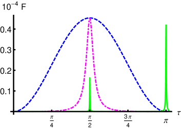
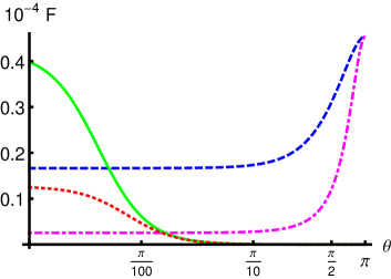
Figure 1: (Color online) Upper panel: FI for $\beta=10$ as a function of the effective time $\tau$, for different $\vartheta$ values: $\vartheta=\pi$ (dashed blue), $\vartheta=0.95\,\pi$ (dot-dashed magenta) and $\vartheta=0$ (solid green). FI takes a pronounced global maximum at $(\vartheta,\tau)=\left(\pi,\frac{\pi}{2}\right)$ while it is possible to see a secondary extremely peaked maximum, which occurs for $\tau=\pi$ and preparing the qubit in $\left|{0}\right\rangle$. Lower panel: log-linear plot of the FI for $\beta=10$ as a function of $\vartheta$ for, $\tau=\frac{\pi}{2}$ (dashed blue), $\tau=\frac{\pi}{2}+\varepsilon$ (dot-dashed magenta), $\tau=\pi$ (solid green), $\tau=\pi+\varepsilon$ (dotted red), with $\varepsilon=0.01$.

Let us now consider the system at a fixed value of the temperature, e.g. where the resonator is supposed to be very close to the ground state, say $\beta=10$. The probabilities $p(j|\beta)=\varrho_{jj}$ evolve periodically in time according to Eq. (12), as the coupled system undergoes Rabi oscillations. The corresponding behavior of the FI is shown in the upper panel of Fig. 1. The FI displays a robust maximum at the optimal time $\tau_{\rm max}=\frac{\pi}{2}$ for $\vartheta=\pi$, corresponding to prepare the qubit in its ground state. This maximum is, at the same time, the global and the smoothest one. In fact, as soon as $\vartheta$ is moved from $\pi$ the FI suddenly drops to zero, except for a sharp peak centered in $\tau_{\rm max}$, monotonically decreasing with respect to $\vartheta$, as shown in the lower panel of Fig. 1. Another maximum of the same order of the global one can be found at $(\vartheta,\tau)=\left(0,\pi\right)$ but it is extremely peaked, thus representing a bad (unstable) choice for a possible measurement. Upon inspecting the temporal evolution of the excited state probability we found that $p(e|\beta)$ has a minimum at $\tau=\tau_{\rm max}$, a fact which gives us a physical insight on the FI behavior: since our goal is the estimation of a vanishing quantity which carries information about thermal disorder, we expect to find the maximum sensitivity in our predictions where the excitation is most likely stored – as a phonon – in the resonator, i.e., when $p(e|\beta)$ is minimum.

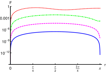
Figure 2: (Color online) Log-linear plot of the FI as a function of effective time $\tau$ for different values of $\beta$. The qubit is prepared in the ground state $\left|{1}\right\rangle$ ($\vartheta=\pi$). From bottom to top $\beta=15$ (solid blue), $\beta=10$ (dashed magenta), $\beta=5$ (dot-dashed green), $\beta=1$ (dotted red). Upon raising the temperature the FI no longer keeps a scale-free shape: thermal excitations modifies its profile making it irregular. In particular the global maximum comes earlier in time.

Let us now turn our attention to the dependence of the FI on the temperature itself. In Fig. 2 we show, on a logarithmic scale, the temporal evolution of the FI for different values of $\beta$. FI varies over several orders of magnitude, matching our intuition that the closer we are to the ground state, the harder is to achieve a given precision in estimation of temperature. Furthermore, upon lowering the temperature, the temporal evolution of $p(j|\beta)$ becomes less involved, finally approaching the exactly periodic one of Rabi oscillations, which in turn freezes the profile of the FI in a shape independent on the temperature itself.

The qubit preparation $\theta=\pi$ is universally optimal, i.e., it leads to a maximum of the FI independently of the interaction time. After fixing $\theta=\pi$ we have numerically maximized $F(\beta)$ with respect to $\tau$. The solid blue line of the upper panel of Fig. 3 is the the log-plot of

$$F_{M}(\beta)=\max_{\tau}F(\beta)\,,$$

as a function of $\beta$, from which it is apparent the exponential decrease of the maximum value achieved by the FI for increasing $\beta$. The Cramér-Rao inequality immediately relates this fact to an exponential loss of sensitivity moving towards the quantum ground state of the resonator. An other interesting feature that emerges from the maximization is a shift in the value of the optimal interaction time. In the lower panel of Fig. 3 we can recognize the existence of a steady value for the optimal time $\tau_{\rm max}=\frac{\pi}{2}$ when approaching the ground state, while for smaller values of $\beta$ the optimal time comes earlier. In fact, the temporal evolution of FI (see Fig. 2) not only predicts an exponential increase of the global maximum when temperatures are raised, but also a shift of its location.

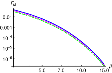
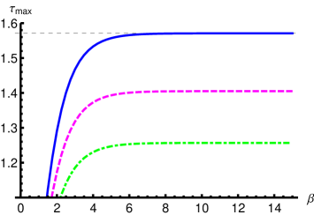
Figure 3: (Color online) Upper panel: log-log plot of the FI maximized over $\tau$ as a function of $\beta$, with $\theta=\pi$ for different values of detuning: $\gamma=0$ (solid blue), $\gamma=1$ (dashed magenta), $\gamma=1.5$ (dot-dashed green). Bottom panel: the times $\tau_{\rm max}$ which maximizes the FI as a function of $\beta$, with $\theta=\pi$ for different values of $\gamma$ (same values and colors of the upper panel).

IV.2 Effects of detuning

In this section we take into account the possible existence of a nonzero detuning $\gamma$ between the oscillator and the qubit frequencies. This has two main consequences, which are both illustrated in Fig. 3. On the one hand, the maximum achievable value of the FI slightly decreases and, on the other hand, the optimal interaction time $\tau_{\rm max}$ at which the maximum takes place anticipates. Therefore, the best working conditions to achieve the optimal sensitivity in the estimation of $\beta$ correspond to have the qubit and the resonator in resonance. It is also worth to notice that $\gamma$ does not represent a critical parameter, as the initial preparation of the qubit, since the FI dependence on $\gamma$ is smooth. One can see this in the upper panel of Fig. 3, where we see that curves corresponding to quite different values of the detuning are almost superposed.

IV.3 Quantum Fisher information

In order to assess the performances of the population measurement in the estimation of temperature we have evaluated the QFI of the family $\varrho_{\scriptscriptstyle P}(\beta)$. The diagonalization of the probe state has to be carried out numerically, hence in general analytical expressions of the QFI are not available. A first fact is that $G(\beta)$ turns out to be independent on the qubit phase $\varphi$, which then does not represent an extra degree of freedom whereby gain more restrictive bounds to precision on $\mbox{Var}(\beta)$. Even the optimal qubit preparation for to the best conceivable measurement involves control of the parameter $\vartheta$ only.

As we have done for the FI, we start to inspect the QFI behavior for a fixed value of temperature $\beta$ in the resonant case. Also for the QFI the maximum is achieved by preparing the qubit in the state $\left|{g}\right\rangle$ and probing it at time $\tau_{\rm max}$. In this case the behavior of $G(\beta)$ is identical to that of $F(\beta)$, as it is apparent by comparing Figs. 1 and 4. In other words, for a given value of the parameter $\beta$ into the range explored, the choice $(\vartheta,\tau)=(\pi,\tau_{\rm max})$ makes population measurement optimal. Moreover, the QFI itself reaches its global maximum for that choice. Thus, provided that an optimal estimator is employed, e.g. maximum likelihood in the asymptotic regime, this strategy provides optimality in sense that either inequality (17) is saturated and the right-hand side of QCR is as low as possible.

This conclusion is confirmed upon a closer inspection of the probe state. When $\vartheta=\pi$ the off-diagonal terms vanish and $\varrho_{\scriptscriptstyle P}$ is diagonal, with eigenvalues

$$\varrho_{+} =\sum_{n=0}^{\infty}p_{n}(\Omega,\beta)\sin^{2}\left[\sqrt{\gamma^{2}+4n}\,\frac{\tau}{2}\right]\frac{n}{n+\gamma^{2}/4}$$ (21a)

$$\varrho_{-} =1-\varrho_{+}$$ (21b)

As a consequence, the QFI reduces to

$$G(\beta;\pi,\tau,\gamma)=\frac{\left(\partial_{\beta}\varrho_{+}\right)^{2}}{\varrho_{+}}+\frac{\left(\partial_{\beta}\varrho_{-}\right)^{2}}{\varrho_{-}}\,,$$

which coincides with the FI ruling the estimation of $\beta$ via population measurement.

On the other hand, some striking difference emerges between the performances of population measurement and that of the optimal one if the qubit is not prepared in the optimal (ground) state.

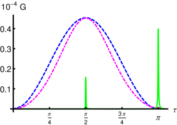
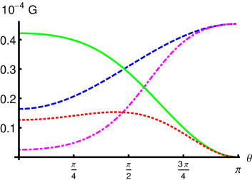
Figure 4: (Color online) Upper panel : QFI for $\beta=10$ as a function of $\tau$, for $\vartheta=\pi$ (dashed blue), $\vartheta=0.95\,\pi$ (dot-dashed magenta) and $\vartheta=0$ (solid green). QFI behaves like FI for $\vartheta=\pi$ leading to the same maximum, while for smaller angles it shows a smoother profile. For angles $0<\vartheta<\pi$ one may find measurements which improve the precision of temperature estimation. Bottom panel: QFI for $\beta=10$ as a function of $\vartheta$ for $\tau=\frac{\pi}{2}$ (dashed blue), $\tau=\frac{\pi}{2}+\varepsilon$ (dot-dashed magenta), $\tau=\pi$ (solid green), $\tau=\pi+\varepsilon$ (dotted red), with $\varepsilon=0.01$.

In the lower panel of Fig. 4 we show $G(\beta)$ as a function of $\tau$ for different values of $\vartheta$: for $\vartheta<\pi$ the decrease of $G$ is definitely smoother than that of $F$ and thus, in principle, some measurement may be found making the initial preparation a less critical parameter. Moreover inspecting the cut of the QFI along $\tau=\pi$ we note that the maximum in $\vartheta=0$ becomes more achievable compared to the one of $F(\beta)$. All these features suggest that for qubit preparations different from the ground state there will be a sensible difference between the precision provided by population measurement and the optimal one implementable on the system. On the other hand, being the overall maximum achievable with population measurement, our results indicate that the achievement of the ultimate bound to precision allowed by quantum mechanics is in the capabilities of the current technology.

IV.4 Effects of decoherence

In this section we discuss the solution of the reduced qubit dynamics in the presence of dissipative decoherence, see Eq. (13), and inspect the corresponding behavior of the FI. For the sake of simplicity we consider zero detuning. Analogue results are obtained when including the detuning.

The probabilities $p(j|\beta)=\tilde{\varrho}_{jj}$ are damped so that, waiting for a sufficient long time, whose value depends on $a$ and $b$, we would find them to be identically $1/2$ or, equally stated, the dynamical evolution brings the state to the maximally mixed one. The contribution of decoherence is of the kind exp$\left[-b(1+n)^{a}\tau\right]$ for every $n$, where $b$ has been rescaled in coupling units $b\longmapsto b/\lambda$. Being a multiplicative coefficient, as soon as $b$ is different from zero, the exponential term will participate in killing the sums. Our calculations show a relevant dependence of the FI on the parameter $b$, namely values $b\approx 10^{-5}$ are sufficient to produce visible effects, while varying $a$ in the range $(0,1)$ does not deeply influence of FI behavior.

In Fig. 5 we show the temporal evolution of the FI for $\beta=10$, in the presence of decoherence and for different initial preparations of the qubit. In the Hamiltonian regime for large $\beta$ the resonator is close to the ground state, the evolution of $p(j|\beta)$ is periodic and hence, due to Eq. (15), the same is true for the FI. Upon incorporating decoherence we see that FI decays at a rate depending on $b$ and thus an irreversible dynamics emerges, which matches the physical evidence of a limited coherence time. On the other hand, a clear maximum at $\tau=\pi/2$ still appears, with a slightly decreased value of $F(\beta)$. In the lower panel of Fig. 5 we show the maximum value $F_{M}=\max_{\tau}F(\beta)$ for different values of the decoherence parameter. As it is apparent from the (log-log) plot for high temperature (smaller $\beta$) the effect of decoherence is negligible, whereas for increasing $\beta$ the effect is becoming more and more relevant.

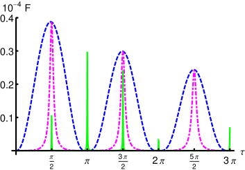
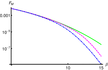
Figure 5: (Color online) Upper panel: Fisher information $F(\beta)$ for $\beta=10$ as a function of $\tau$ in the presence of decoherence and for different qubit preparations. The decoherence parameters are chosen as to $a=0.1$ and $b=10^{-5}$. Dashed blue line stands for $\vartheta=\pi$, dot-dashed magenta for $\vartheta=0.95\,\pi$ while solid green ones for $\vartheta=0$. Having included decoherence treatment enables us not to restrict the evolution to the first Rabi half-period. Lower panel: log-log plot of the Fisher information $F_{M}(\beta)$ maximized over the interaction time, and in the presence of decoherence, as a function of $\beta$ and for fixed $\vartheta=\pi$, for $b=0$ (solid green), $b=10^{-5}$ (dashed magenta), $b=10^{-4}$ (dot-dashed blue).

V Conclusions

The temperature of a physical object cannot be directly measurable. On the other hand is can be regarded as a parameter whose value can be indirectly inferred by measuring some proper observable and then suitably processing the outcomes, an inference procedure usually referred to as an estimation procedure. In the case of a micromechanical oscillator with an isolated vibrational mode, effective schemes have been suggested and realized nmr11 which rely on coupling the resonator to a superconducting qubit and probing the latter using population measurements. In other words, the qubit is employed as a quantum thermometer to demonstrate that the resonator has been cooled to its quantum ground state. In this paper we have analyzed in details qubit thermometry in these systems, i.e., the estimation of temperature via quantum limited measurements performed on the qubit. In the framework of quantum estimation theory we have analyzed precision as a function of both the qubit initial preparation and the interaction parameters, and we have evaluated the limits to precision posed by quantum mechanics to qubit thermometry.

We have computed the FI for population measurement, which is the appropriate figure of merit to assess the precision of estimation, and have found that its maximum, and hence the minimum variance in the estimated temperature, is achieved by preparing the qubit in the ground state, and probing it at an emergent time $\tau_{\rm max}$, which is predictable. Furthermore, we have analyzed in details how the maximum depends on the temperature itself, on the detuning, and on the noise parameter when one takes into account non dissipative decoherence. In order to evaluate the ultimate bound allowed by quantum mechanics to the sensitivity of temperature estimation, we have also computed the quantum Fisher information. We found that QFI is maximized for the same choice of qubit preparation and measurement time of the FI, and that for these common values the maxima of FI and QFI coincide. We thus conclude that population measurement is optimal for temperature estimation.

The range of parameters addressed in our analysis is that of recent experimental implementations nmr11 . We thus conclude that optimal estimation of temperature can be done with current technology. Since the FI of population measurement, and the QFI of the model, both decrease with the decrease of temperature, the estimation of lower temperature will be intrinsically less precise. On the other hand, since the are regimes, also in the presence of decoherence, where the maxima of the FI and the QFI are reasonably smooth as a function of the qubit preparation and of the interaction time we do not expect any ”no-go” theorem for temperature estimation. In other words, we expect that optimal estimation of lower resonator temperatures, perhaps achievable with further experimental advances, will be still possible with population measurements. On the other hand, “optimality” will correspond to an inherently less precise procedure compared to the case of higher temperature.

Our analysis shows the optimality of feasible qubit thermometry in providing quantum benchmarks for high precision temperature measurement, as well as an efficient operational quantification of temperature for mechanical modes lying arbitrary close to their ground state. In other words, achievement of the ultimate bound to precision allowed by quantum mechanics is in the capabilities of the current technology. Our results also confirm that QET is a useful tool for assessing and comparing inference procedures arising in quantum limited measurements sta10 , even when mesoscopic objects are involved.

References

- (1) J. M. Courty, A. Heidmann, M. Pinard, Eur. Phys. J. D 17, 399408 (2001).
- (2) A. D. Armour, M. P. Blencowe, K. C. Schwab, Phys. Rev. Lett. 88, 148301 (2002).
- (3) A. N. Cleland, M. R. Geller, Phys. Rev. Lett. 93, 070501 (2004).
- (4) M. D. LaHaye, P. Buu, B. Camarota, K. C. Schwab, Science 304, 7477 (2004).
- (5) M. Blencowe, Phys. Rep. 395, 159222 (2004).
- (6) I. Martin, A. Shnirman, L. Tian, P. Zoller, Phys. Rev. B 69, 125339 (2004).
- (7) D. Kleckner, D. Bouwmeester, Nature 444, 7578 (2006).
- (8) A. Schliesser, R. Riviere, G. Anetsberger, O. Arcizet, T. J. Kippenberg Nature Phys. 4, 415419 (2008).
- (9) C. A. Regal, J. D. Teufel, K. W. Lehnert, Nature Phys. 4, 555560 (2008).
- (10) T. Rocheleau, T. Ndukum, C. Macklin, J. B. Hertzberg, A. A. Clerk, K. C. Schwab, Nature 463, 7275 (2010).
- (11) A. D. O’Connell1, M. Hofheinz, M. Ansmann, R. C. Bialczak1, M. Lenander, E. Lucero, M. Neeley, D. Sank, H. Wang, M. Weides, J. Wenner, J. M. Martinis, A. N.Cleland, Nature 464, 697 (2010).
- (12) A. Monras, Phys. Rev. A 73, 033821 (2006).
- (13) S. Olivares, M. G A Paris, J. Phys. B 42, 055506 (2009).
- (14) M. Aspachs, J. Calsamiglia, R. Munoz-Tapia, E. Bagan, Phys. Rev. A 79, 033834 (2009).
- (15) M. G. Genoni, S. Olivares, M. G. A. Paris Phys. Rev. Lett. 106, 153603 (2011).
- (16) M. G. Genoni, P. Giorda, M. G A Paris, Phys. Rev. A 78, 032303 (2008).
- (17) G. Brida, I. P. Degiovanni, A. Florio, M. Genovese, P. Giorda, A. Meda, M. G. A. Paris, A. Shurupov, Phys. Rev. Lett. 104, 100501 (2010).
- (18) G. Brida, I. P. Degiovanni, A. Florio, M. Genovese, P. Giorda, A. Meda, M. G. A. Paris, A. P. Shurupov, Phys. Rev. A 83, 052301 (2011).
- (19) M. Sarovar and G. Milburn, J. Phys. A 39, 8487 (2006).
- (20) M. Hotta, T. Karasawa, M. Ozawa, Phys. Rev. A 72, 052334 (2005).
- (21) A. Monras, M. G. A. Paris, Phys. Rev. Lett. 98, 160401 (2007).
- (22) A. Fujiwara, Phys. Rev. A 65, 012316 (2001).
- (23) Z. Ji, G. Wang, R. Duan, Y. Feng, M. Ying, IEEE Trans. Inf. Theory 54, 5172 (2008).
- (24) S. Boixo, A. Monras, Phys. Rev. Lett. 100, 100503 (2008).
- (25) P. Zanardi, M. G. A. Paris, L. Campos-Venuti, Phys. Rev. A 78, 042105 (2008); C. Invernizzi, M. Korbmann, L. Campos-Venuti, M. G. A. Paris Phys. Rev. A 78, 042106 (2008).
- (26) S. Campbell, M. Paternostro, S. Bose, M. S. Kim, Phys. Rev. A 81, 050301(R) (2010).
- (27) M. Paternostro, S. Gigan, M. S. Kim, F. Blaser, H. R. Bohm, M. Aspelmeyer. New J. Phys. 8, 107 (2006).
- (28) A. Monras, F. Illuminati, Phys. Rev. A 81, 062326 (2010).
- (29) A. Monras, F. Illuminati, Phys. Rev. A 83, 012315 (2011).
- (30) B. B. Mandelbrot, Ann. Math. Stat. 33 1021 (1962); J. Math. Phys. 5, 164 (1964); Phys. Today, January, 71 (1989).
- (31) D. M. Meekhof, C. Monroe, B. E. King, W. M. Itano, D. J. Wineland, Phys. Rev. Lett 76, 1796 (1996).
- (32) C. W. Helstrom, Quantum Detection and Estimation Theory (Academic Press, New York, 1976); A.S. Holevo, Statistical Structure of Quantum Theory, Lect. Not. Phys 61, (Springer, Berlin, 2001).
- (33) S. L. Braunstein, C. M. Caves, Phys. Rev. Lett. 72 3439 (1994); S. L. Braunstein, C. M. Caves, G. J. Milburn, Ann. Phys. 247, 135 (1996).
- (34) A. Fujiwara, METR 94-08 (1994).
- (35) D. C. Brody, L. P. Hughston, Proc. Roy. Soc. Lond. A 454, 2445 (1998); A 455, 1683 (1999).
- (36) S. Amari and H. Nagaoka, Methods of Information Geometry, Trans. Math. Mon. 191, AMS (2000).
- (37) M. G A Paris, Int. J. Quant. Inf. 7, 125 (2009).
- (38) J. Gemmer, M. Michel, G. Mahler, Quantum Thermodynamics, Lect. Not. Phys. 784 (2009).
- (39) C. H. Webster, NPL Report DEM-TQD-007 (2006).
- (40) T. Jahnke, S. Lanery, G. Mahler, Phys. Rev. E 83, 011109 (2011).
- (41) T. L. Schmidt, K. Borkje, C. Bruder, B. Trauzettel, Phys. Rev. Lett. 104, 177205 (2010).
- (42) T. M. Stace, Phys. Rev. A 82, 011611 (2010).