Path-integral calculation of the third virial coefficient of quantum gases at low temperatures

Abstract

We derive path-integral expressions for the second and third virial coefficients of monatomic quantum gases. Unlike previous work that considered only Boltzmann statistics, we include exchange effects (Bose–Einstein or Fermi–Dirac statistics). We use state-of-the-art pair and three-body potentials to calculate the third virial coefficient of ³He and ⁴He in the temperature range $2.6-24.5561$ K. We obtain uncertainties smaller than those of the limited experimental data. Inclusion of exchange effects is necessary to obtain accurate results below about 7 K.

I Introduction

Thermodynamic properties of fluids at very low temperatures are of significant interest. For example, the current International Temperature Scale Preston-Thomas (1990) makes use of volumetric properties and vapor pressures of helium isotopes below the triple point of neon (24.5561 K); below the triple point of hydrogen (13.8033 K), the scale is based entirely on properties of ³He and ⁴He. The theoretical analysis of relevant properties at these conditions, such as the virial coefficients that describe the fluid’s departure from ideal-gas behavior, is complicated by the presence of quantum effects.

The inclusion of quantum effects in the calculation of virial coefficients was one of the first numerical applications of the Path-Integral Monte Carlo (PIMC) method. Feynman and Hibbs (1965) In a series of pioneering works published in the 1960’s, Fosdick and Jordan showed how to calculate the second and third virial coefficient of a monatomic gas using computer simulations. Fosdick and Jordan (1966); Jordan and Fosdick (1968); Fosdick (1968) Given the limited computational resources available at that time, they were able to calculate the third virial coefficient only in the case of two-body interactions, using a model potential of the Lennard-Jones form and assuming distinguishable particles (Boltzmann statistics). They argued that their method could be extended to include the proper quantum statistics, but they were able to compute exchange effects only in the case of the second virial coefficient.

Recently, the exponential increase in computational power has enabled use of the path-integral method to calculate the properties of quantum degenerate systems, notably superfluid helium. Ceperley (1995) At the same time, progress in the computation of ab initio electronic properties of interacting atoms resulted in the availability of very precise two- and three-body interparticle potentials, at least for the lightest particles such as helium atoms Jeziorska et al. (2007); Hellmann, Bich, and Vogel (2007); Cencek et al. (2007); Cencek, Patkowski, and Szalewicz (2009); Przybytek et al. (2010) or hydrogen molecules. Diep and Johnson (2000); Patkowski et al. (2008)

A natural application for these potentials is the calculation of virial coefficients. As is well known, the second virial coefficient depends only on the two-body potential, the third virial coefficient depends only on two-body and three-body interactions, etc. The second virial coefficient for a monatomic gas can be rigorously obtained at the fully quantum level from the calculation of the phase shifts due to the pair potential, and previous work has shown that a completely ab initio calculation of second virial coefficients for helium can have uncertainties comparable to and in many cases smaller than those of the most precise experiments. Hurly and Mehl (2007); Hurly and Moldover (2000); Bich, Hellmann, and Vogel (2007); Mehl (2009); Cencek et al. (tion)

In the case of the third virial coefficient, no closed-form solution of the quantum statistical mechanics problem is known. First-order semiclassical approaches have been derived Yokota (1960); Ram and Singh (1973) and show that, in the case of helium, quantum diffraction effects result in significant modifications of the classical result, even at room temperature. However, there is no rigorous way to evaluate the accuracy or uncertainty of the semiclassical result, especially at low temperatures.

In recent work, Garberoglio and Harvey (2009) we extended the methodology pioneered by Fosdick and Jordan, deriving a set of formulae allowing a path-integral calculation of the third virial coefficient $C(T)$ of monatomic species for arbitrary two- and three-body potentials. Our results were limited to Boltzmann statistics (i.e., distinguishable particles) and we did not present results for temperatures lower than the triple point of neon ($24.5561$ K), which we deemed to be a reasonable lower bound so that exchange effects could be neglected. Nevertheless, we were able to compute the value of the third virial coefficient of ⁴He with an uncertainty one order of magnitude smaller than that of the best experiments.

Recent experimental results overlapping with our temperature range, Gaiser and Fellmuth (2009); Gaiser, Fellmuth, and Haft (2010) although mostly consistent with our calculations, seemed to indicate a systematic deviation which the authors speculated could originate from our neglect of the proper quantum statistics of helium atoms.

In this paper, we extend our computational methodology to calculate the quantum statistical contributions to the third virial coefficient, and compute $C(T)$ for both isotopes of helium in the temperature range $2.6-24.5561$ K, extending the temperature range considered in our previous work down into the range where exchange effects are important. We show that quantum statistical effects are significant only for temperatures smaller than about $7$ K, and compare our results to low-temperature experimental data.

In a subsequent publication Garberoglio, Moldover, and Harvey (tion), we will present results covering the entire temperature range (improving on our previous results for ⁴He at 24.5561 K and above) with rigorously derived uncertainties. We will also extend our methodology to include acoustic virial coefficients, and compare those calculations to available data. In the present work, our focus is on low temperatures and specifically on the effect of non-Boltzmann statistics.

II Path-integral calculation of the virial coefficients

The second and third virial coefficients, $B(T)$ and $C(T)$ respectively, are given by Hirschfelder, Curtiss, and Bird (1954)

$$B(T) = -\frac{1}{2V}\left(Z_{2}-Z_{1}^{2}\right)$$ (1)

$$C(T) = 4B^{2}(T)-\frac{1}{3V}\left[Z_{3}-3Z_{2}Z_{1}+2Z_{1}^{3}\right],$$ (2)

where $V$ is the integration volume (with the limit $V\rightarrow\infty$ taken at the end of the calculations), and the functions $Z_{N}$ are given by:

$$Z_{3} = \Lambda^{9}\int\mathrm{d}1\mathrm{d}2\mathrm{d}3~{}\langle 123|\mathrm{e}^{-\beta\hat{H}_{3}}\sum_{\pi_{3}}{\cal P}_{\pi_{3}}|123\rangle$$ (3)

$$Z_{2} = \Lambda^{6}\int\mathrm{d}1\mathrm{d}2~{}\langle 12|\mathrm{e}^{-\beta\hat{H}_{2}}\sum_{\pi_{2}}{\cal P}_{\pi_{2}}|12\rangle$$ (4)

$$Z_{1} = \Lambda^{3}\int\mathrm{d}1~{}\langle 1|\mathrm{e}^{-\beta\hat{H}_{1}}|1\rangle=V,$$ (5)

where $\hat{H}_{N}$ is the $N$-body Hamiltonian, $\beta=1/(k_{\mathrm{B}}T)$, ${\cal P}$ is a permutation operator (multiplied by the sign of the permutation in the case of Fermi–Dirac statistics), the index $\pi_{3}$ runs over the 6 permutations of 3 objects (i.e., $123$, $132$, $213$, $321$, $231$ and $312$), and $\pi_{2}$ runs over the 2 permutations of 2 objects (i.e., $12$ and $21$). $\Lambda=h/\sqrt{2\pi mk_{\mathrm{B}}T}$ is the thermal de Broglie wavelength of a particle of mass $m$ at temperature $T$. For the sake of conciseness, we denote by $|i\rangle$ an eigenvector of the position operator relative to particle $i$ and by $\mathrm{d}i$ ($i=1,2,3$) the integration volume relative to the Cartesian coordinates of the $i$-th particle. Note that, in order to produce the molar units used by experimenters and in our subsequent comparisons with data, the right side of Eq. (1) and the second term in the right side of Eq. (2) must be multiplied by Avogadro’s number and its square, respectively.

In the following, we will derive a path-integral expression for the calculation of the virial coefficients with Eqs. (1) and (2). We perform the derivation in detail in the case of $B(T)$ to establish the notation, and then extend the results to the more interesting case of $C(T)$.

II.1 Second virial coefficient

In this paper, we adopt Cartesian coordinates to describe the atomic positions. This differs from the approach developed in Refs. Jordan and Fosdick, 1968 and Garberoglio and Harvey, 2009, where Jacobi coordinates were used. This choice allows the exchange contribution to be computed in a much simpler manner than would be the case if Jacobi coordinates were used, especially in the case of three or more particles.

From Eqs. (1) and (4), it can be seen that there are two contributions to $B(T)$. The first one comes from considering the identity permutation only, and takes into account only quantum diffraction effects. This is the only contribution that gives a nonzero result at high temperatures, where the particles can be treated as distinguishable (Boltzmann statistics).

The second contribution to $B(T)$, which we will call exchange (xc), comes from the only other permutation involved in the definition of the quantity $Z_{2}$ above.

The expression of these two contributions in Cartesian coordinates is:

$$B_{\mathrm{Boltzmann}}(T) = -\frac{\Lambda^{6}}{2V}\int\mathrm{d}\boldsymbol{r}_{1}\mathrm{d}\boldsymbol{r}_{2}~{}\langle\boldsymbol{r}_{1}\boldsymbol{r}_{2}|\exp\left[-\beta(\hat{K}_{2}+\hat{U}_{2}(|\boldsymbol{r}_{2}-\boldsymbol{r}_{1}|))\right]-\exp\left[-\beta\hat{K}_{2}\right]|\boldsymbol{r}_{1}\boldsymbol{r}_{2}\rangle$$ (6)

$$B_{\mathrm{xc}}(T) = -\frac{(-1)^{2I}\Lambda^{6}}{(2I+1)2V}\int\mathrm{d}\boldsymbol{r}_{1}\mathrm{d}\boldsymbol{r}_{2}\langle\boldsymbol{r}_{1}\boldsymbol{r}_{2}|\exp\left[-\beta(\hat{K}_{2}+\hat{U}_{2}(|\boldsymbol{r}_{2}-\boldsymbol{r}_{1}|))\right]|\boldsymbol{r}_{2}\boldsymbol{r}_{1}\rangle,$$ (7)

where we denote by $K_{N}$ the total kinetic energy of $N$ bodies and by $\hat{U}_{2}(r)$ the two-body potential energy operator and $I$ is the nuclear spin of the atomic species under consideration ($I=0$ for ⁴He and $I=1/2$ for ³He).

Equations (6) and (7) can be rewritten by using the Trotter identity

$$\mathrm{e}^{\hat{K}_{2}+\hat{U}_{2}}=\lim_{P\rightarrow\infty}\left(\mathrm{e}^{\hat{K}_{2}/P}\mathrm{e}^{\hat{U}_{2}/P}\right)^{P}$$ (8)

with a positive integer value of the Trotter index $P$.

Following the procedure outlined in Ref. Garberoglio and Harvey, 2009, one can then write $B_{\mathrm{Boltzmann}}(T)$ as

$$B_{\mathrm{Boltzmann}}(T)=-2\pi^{2}\int_{0}^{\infty}r^{2}\mathrm{d}r~{}\left(\exp\left[-\beta\overline{U}_{2}(r)\right]-1\right),$$ (9)

where the two-body effective potential $\overline{U}_{2}(r)$ is given by

$$\exp\left[-\beta\overline{U}_{2}(r)\right] = \int\prod_{i=1}^{P-1}\mathrm{d}\Delta\boldsymbol{x}_{1}^{(i)}\mathrm{d}\Delta\boldsymbol{x}_{2}^{(i)}~{}\exp\left[-\frac{\beta}{P}\sum_{i=1}^{P}U_{2}(|\boldsymbol{r}+\boldsymbol{x}_{2}^{(i)}-\boldsymbol{x}_{1}^{(i)}|)\right]\times$$ (10)

$$F_{\mathrm{ring}}(\Delta\boldsymbol{x}_{1}^{(1)},\ldots,\Delta\boldsymbol{x}_{1}^{(P)})F_{\mathrm{ring}}(\Delta\boldsymbol{x}_{2}^{(1)},\ldots,\Delta\boldsymbol{x}_{2}^{(P)})$$

$$\underset{P\rightarrow\infty}{=} \oint{\cal D}\boldsymbol{x}_{1}{\cal D}\boldsymbol{x}_{2}~{}\exp\left[-\frac{1}{\hbar}\int_{0}^{\beta\hbar}\frac{m}{2}\left|\frac{\mathrm{d}\boldsymbol{x}_{1}(\tau)}{\mathrm{d}\tau}\right|^{2}+\frac{m}{2}\left|\frac{\mathrm{d}\boldsymbol{x}_{2}(\tau)}{\mathrm{d}\tau}\right|^{2}~{}+U_{2}(|\boldsymbol{r}+\boldsymbol{x}_{1}(\tau)-\boldsymbol{x}_{2}(\tau)|)\mathrm{d}\tau\right],$$ (11)

where

$$F_{\mathrm{ring}}=\Lambda^{3}\left(\frac{P^{3/2}}{\Lambda^{3}}\right)^{P}\exp\left[-\frac{\pi P}{\Lambda^{2}}\sum_{i=1}^{P}\left|\Delta\boldsymbol{x}_{1}^{(i)}\right|^{2}\right].$$ (12)

In the previous equations, we have defined $\Delta\boldsymbol{x}_{k}^{(i)}=\boldsymbol{r}_{k}^{(i+1)}-\boldsymbol{r}_{k}^{(i)}$, where $\boldsymbol{r}_{k}^{(i)}$ is the coordinate of particle $k$ ($k=1,2$) in the $i$-th “imaginary time slice”. These “slices” are obtained by inserting $P$ completeness relations of the form

$$1=\int\mathrm{d}\boldsymbol{r}_{1}^{(i)}\mathrm{d}\boldsymbol{r}_{2}^{(i)}~{}|\boldsymbol{r}_{1}^{(i)}\boldsymbol{r}_{2}^{(i)}\rangle\langle\boldsymbol{r}_{1}^{(i)}\boldsymbol{r}_{2}^{(i)}|$$ (13)

between the factors $\mathrm{e}^{\hat{K}_{2}/P}$ and $\mathrm{e}^{\hat{U}_{2}/P}$ of the Trotter expansion of Eq. (8). We used the overall translation invariance of the system to remove the factor $V$ in Eq. (6) and fix the $\tau=0$ slice of particle 2 at the origin of the coordinate system. We also denoted by $\boldsymbol{x}_{1}^{(i)}$ and $\boldsymbol{x}_{2}^{(i)}$ the coordinates of two ring polymers having one of their endpoints fixed at the origin ($\boldsymbol{x}_{1}^{(1)}=\boldsymbol{x}_{2}^{(1)}=\mathbf{0}$), and we introduced the variable $\boldsymbol{r}$ denoting the distance between the $\tau=0$ time slice of the two ring polymers. In the classical limit, where the paths $\boldsymbol{x}_{1}(\tau)$ and $\boldsymbol{x}_{2}(\tau)$ shrink to a point, the coordinate $r$ reduces to the distance between the particles and one has $\overline{U}_{2}(r)=U_{2}(r)$.

Note that the effect of the identity permutation is to set $\boldsymbol{r}_{k}^{(P+1)}=\boldsymbol{r}_{k}^{(1)}$. The path-integral formalism allows one to map the quantum statistical properties of a system with $N$ distinguishable particles (Boltzmann statistics) onto the classical statistical properties of a system of $N$ ring polymers, each having $P$ beads (sometimes called imaginary-time slices), which are distributed according to the function $F_{\mathrm{ring}}$ of Eq. (12). Garberoglio (2008) The mapping is exact in the $P\rightarrow\infty$ limit, although convergence is usually reached with a finite (albeit large) value of $P$.

In the calculation of the second virial coefficient, Eq. (9) shows that the second virial coefficient at the level of Boltzmann statistics is obtained from an expression similar to that for the classical second virial coefficient, using an effective two-body potential. This effective potential, $\overline{U}_{2}(r)$, is obtained by averaging the intermolecular potential $U_{2}(r)$ over the coordinates of two ring polymers, corresponding to the two interacting particles entering the definition of $B(T)$.

Equation (9) is equivalent to Eq. (19) of Ref. Garberoglio and Harvey, 2009. The only difference is that the current approach uses Cartesian coordinates, and therefore we are left with an average over two ring polymers of mass $m$ instead of one ring polymer of mass $\mu=m/2$, corresponding to the relative coordinate of the two-particle system. The two approaches are of course equivalent, and in fact it can be shown that Eqs. (9) and (10) reduce to the form derived in Refs. Fosdick and Jordan, 1966 and Garberoglio and Harvey, 2009. Equation (9) is the same expression previously derived by Diep and Johnson for spherically symmetric potentials on the basis of heuristic arguments, Diep and Johnson (2000) and later generalized by Schenter to the case of rigid bodies and applied to a model for water. Schenter (2002)

Equation (10) is actually the discretized version of a path integral, as shown in Eq. (11). The circled integral is defined as

$$\oint{\cal D}\boldsymbol{x}~{}\exp\left[-\frac{1}{\hbar}\int_{0}^{\beta\hbar}\frac{m}{2}\left|\frac{\mathrm{d}\boldsymbol{x}(\tau)}{\mathrm{d}\tau}\right|^{2}~{}\mathrm{d}\tau\right] \equiv$$

$$\lim_{P\rightarrow\infty}\int\prod_{i=1}^{P-1}\mathrm{d}\Delta\boldsymbol{x}^{(i)}F_{\mathrm{ring}}(\Delta\boldsymbol{x}^{(1)},\ldots,\Delta\boldsymbol{x}^{(P)}) = 1,$$ (14)

and it indicates that one has to consider all the cyclic paths with ending points at the origin, that is $\boldsymbol{x}(0)=\boldsymbol{x}(\beta\hbar)=\boldsymbol{0}$. The normalization of the path integral is also indicated in Eq. (14).

We can perform on Eq. (7), describing the exchange contribution to the second virial coefficient, the same steps leading from Eq. (6) to Eq. (9). The only difference is the presence of the permutation operator, whose main consequence is fact that $\boldsymbol{r}^{(P+1)}_{1}=\boldsymbol{r}^{(1)}_{2}$ and $\boldsymbol{r}^{(P+1)}_{2}=\boldsymbol{r}^{(1)}_{1}$. In this case, defining $\boldsymbol{X}^{(i)}=\boldsymbol{r}^{(i)}_{1}$ and $\boldsymbol{X}^{(i+P)}=\boldsymbol{r}^{(i)}_{2}$, one obtains

$$B_{\mathrm{xc}}(T) = -\frac{(-1)^{2I}\Lambda^{6}}{2(2I+1)V}\int\mathrm{d}\boldsymbol{X}^{(1)}\ldots\mathrm{d}\boldsymbol{X}^{(2P)}~{}\exp\left[-\frac{\beta}{P}\sum_{i=1}^{P}U_{2}(|\boldsymbol{X}^{(P+i)}-\boldsymbol{X}^{(i)}|)\right]\times$$ (16)

$$\left(\frac{P^{3/2}}{\Lambda^{3}}\right)^{2P}\exp\left[-\frac{\pi P}{\Lambda^{2}}\sum_{i=1}^{2P}\left(\boldsymbol{X}^{(i+1)}-\boldsymbol{X}^{(i)}\right)^{2}\right]$$

$$= -\frac{(-1)^{2I}\Lambda^{3}}{2(2I+1)V}\int\mathrm{d}\boldsymbol{X}^{(1)}\ldots\mathrm{d}\boldsymbol{X}^{(2P)}~{}\exp\left[-\frac{\beta}{P}\sum_{i=1}^{P}U_{2}(|\boldsymbol{X}^{(P+i)}-\boldsymbol{X}^{(i)}|)\right]\times$$

$$\frac{\Lambda_{\mu}^{3}}{2^{3/2}}\left(\frac{(2P)^{3/2}}{\Lambda_{\mu}^{3}}\right)^{2P}\exp\left[-\frac{\pi~{}2P}{\Lambda_{\mu}^{2}}\sum_{i=1}^{2P}\left(\boldsymbol{X}^{(i+1)}-\boldsymbol{X}^{(i)}\right)^{2}\right]$$

$$= -\frac{1}{2}\frac{(-1)^{2I}\Lambda^{3}}{(2I+1)~{}2^{3/2}}\left\langle\exp\left[-\frac{\beta}{P}\sum_{i=1}^{P}U_{2}(|\boldsymbol{X}^{(P+i)}-\boldsymbol{X}^{(i)}|)\right]\right\rangle$$ (17)

$$\underset{P\rightarrow\infty}{=} -\frac{(-1)^{2I}\Lambda^{3}}{(2I+1)~{}2^{5/2}}~{}\oint{\cal D}\boldsymbol{X}~{}\exp\left[-\frac{1}{\hbar}\int_{0}^{\beta\hbar}\frac{\mu}{2}\left|\frac{\mathrm{d}\boldsymbol{X}(\tau)}{\mathrm{d}\tau}\right|^{2}+U_{2}(|\boldsymbol{X}(\tau+\beta\hbar/2)-\boldsymbol{X}(\tau)|)~{}\mathrm{d}\tau\right],$$ (18)

where we have defined $\Lambda_{\mu}=\sqrt{2}\Lambda$. The exchange contribution to the second virial coefficient is given simply as an average of the two-body potential taken on ring polymers corresponding to particles of mass $\mu=m/2$. In the discretized version of the path integral, one has to consider $2P$ beads. In Eq. (17), we have used the overall translation invariance of the integral to remove the factor of $V$ in the denominator.

The effect of the various permutations can be visualized as generating paths with a larger number of beads, which are obtained by coalescing the ring polymers corresponding to the particles that are exchanged by the permutation operator.

II.2 Third virial coefficient

We now discuss the third virial coefficient, starting from the expression given in Eq. (2). Since $4B^{2}(T)$ can be calculated by the methods of the previous section, we concentrate on the second term, whose summands can be written as follows:

$$Z_{3} = \Lambda^{9}\int\mathrm{d}1\mathrm{d}2\mathrm{d}3~{}\langle 123|\mathrm{e}^{-\beta\hat{H}_{3}}\sum_{\pi_{3}}{\cal P}_{\pi_{3}}|123\rangle$$ (19)

$$Z_{2}Z_{1} = \Lambda^{9}\int\mathrm{d}1\mathrm{d}2\mathrm{d}3~{}\langle 123|\mathrm{e}^{-\beta(\hat{H}_{2}+\hat{T}_{3})}\sum_{\pi_{2}}{\cal P}_{\pi_{2}}|123\rangle$$ (20)

$$Z_{1}^{3} = \Lambda^{9}\int\mathrm{d}1\mathrm{d}2\mathrm{d}3~{}\langle 123|\mathrm{e}^{-\beta\hat{K}_{3}}|123\rangle,$$ (21)

where $\hat{T}_{i}=-\frac{\hbar^{2}}{2m}\nabla_{i}^{2}$ is the kinetic energy operator of particle $i$.

We can simplify the expression in square brackets on the right-hand side of Eq. (2) by writing the three $Z_{2}Z_{1}$ terms choosing each time a different particle for $Z_{1}$ (in Eq. (20) we have chosen particle 3 as coming from $Z_{1}$). After considering all the permutations of two and three particles, we end up with $6+3\times 2+1=13$ terms building the term in square brackets of Eq. (2). It is useful to collect these 13 terms as follows:

1. Term 1 (identity term): we sum together permutation $123$ from $Z_{3}$, the identity permutations from the three $Z_{2}Z_{1}$ and the whole $2Z_{1}^{3}$ term. Adding $4B^{2}_{\rm Boltzmann}(T)$, one obtains the Boltzmann expression for $C(T)$, already discussed in Ref. Garberoglio and Harvey, 2009. In the present formulation based on Cartesian coordinates, the value $C(T)$ in the case of Boltzmann statistics involves an average over three independent ring polymers, which correspond to the three particles. In the following, this contribution to $C(T)$ will be referred to as $C_{\rm Boltzmann}(T)$ and is made by $1+3+1=5$ of the 13 terms described above.

2. Term 2 (odd term): we take permutations $132$, $213$ and $321$ from $Z_{3}$ and the three exchange permutations from the $Z_{2}Z_{1}$ terms. These permutations are all odd, and they have to be multiplied by $(-1)^{2I}/(2I+1)$. All of these permutations correspond to configurations where two of the three particles are exchanged. The sum of these 6 terms will be referred to as $C_{\rm odd}(T)$.

3. Term 3 (even term): we take the permutations $231$ and $312$ from $Z_{3}$. These are the remaining two terms from the 13, and are both even permutations, hence the name. Both of these terms correspond to a cyclic exchange of the three particles, and their sum will be referred to as $C_{\rm even}(T)$. They are to be weighted with $1/(2I+1)^{2}$.

Using these definitions, the full $C(T)$, including quantum statistical effects, can be written as

$$C(T)=C_{\rm Boltzmann}(T)+(-1)^{2I}\frac{C_{\rm odd}(T)}{2I+1}+\frac{C_{\rm even}(T)}{(2I+1)^{2}}+C_{\rm B}(T),$$ (22)

where the last term in the right-hand sum is given by

$$C_{\rm B}(T)=8B_{\rm Boltzmann}(T)B_{\mathrm{xc}}(T)+4B^{2}_{\mathrm{xc}}(T),$$ (23)

since the contribution of $4B^{2}_{\mathrm{Boltzmann}}(T)$ to $C(T)$ is already included in $C_{\rm Boltzmann}(T)$. In Eqs. (22) and (23), the upper (lower) sign corresponds to Bose–Einstein (Fermi–Dirac) statistics.

Using the same procedure outlined above in the case of $B(T)$, one can write the Boltzmann contribution to the third virial coefficient as

$$C_{\mathrm{Boltzmann}}(T) = 4B^{2}_{\mathrm{Boltzmann}}(T)-$$ (24)

$$\frac{1}{3}\int\mathrm{d}\boldsymbol{r}_{1}\mathrm{d}\boldsymbol{r}_{2}\left[\mathrm{e}^{-\beta\overline{V}_{3}(\boldsymbol{r}_{1},\boldsymbol{r}_{2})}-\mathrm{e}^{-\beta\overline{U}_{2}(|\boldsymbol{r}_{1}|)}-\mathrm{e}^{-\beta\overline{U}_{2}(|\boldsymbol{r}_{2}|)}-\mathrm{e}^{-\beta\overline{U}_{2}(|\boldsymbol{r}_{1}-\boldsymbol{r}_{2}|)}+2\right],$$

$$\exp\left[-\beta\overline{V}_{3}(\boldsymbol{r}_{1},\boldsymbol{r}_{2})\right] = \int\prod_{i=1}^{P-1}\Delta\boldsymbol{x}_{1}^{(i)}\Delta\boldsymbol{x}_{2}^{(i)}\Delta\boldsymbol{x}_{3}^{(i)}~{}F_{\mathrm{ring}}^{(1)}F_{\mathrm{ring}}^{(2)}F_{\mathrm{ring}}^{(3)}~{}\exp\left[-\beta\overline{V}_{3}^{\mathrm{B}}(\boldsymbol{r}_{1},\boldsymbol{r}_{2})\right]$$ (26)

$$\underset{P\rightarrow\infty}{=} \oint{\cal D}\boldsymbol{x}_{1}{\cal D}\boldsymbol{x}_{2}{\cal D}\boldsymbol{x}_{3}~{}\exp\left[-\frac{1}{\hbar}\int_{0}^{\beta\hbar}\frac{m}{2}\left(\left|\frac{\mathrm{d}\boldsymbol{x}_{1}(\tau)}{\mathrm{d}\tau}\right|^{2}+\left|\frac{\mathrm{d}\boldsymbol{x}_{2}(\tau)}{\mathrm{d}\tau}\right|^{2}+\left|\frac{\mathrm{d}\boldsymbol{x}_{3}(\tau)}{\mathrm{d}\tau}\right|^{2}\right)+\right.$$

$$\left.V_{3}(\boldsymbol{r}_{1}+\boldsymbol{x}_{1}(\tau),\boldsymbol{r}_{2}+\boldsymbol{x}_{2}(\tau),\boldsymbol{x}_{3}(\tau))~{}\mathrm{d}\tau\right],$$

where $F_{\mathrm{ring}}^{(k)}$ denotes the probability distribution of the path relative to particle $k$, as defined in Eq. (12). In Eq. (26), the three-body effective potential energy $\overline{V}_{3}$ is obtained as an average performed over three independent ring polymers of the total three-body potential energy:

$$V_{3}(\boldsymbol{x},\boldsymbol{y},\boldsymbol{z}) = U_{3}(\boldsymbol{x},\boldsymbol{y},\boldsymbol{z})+U_{2}(|\boldsymbol{x}-\boldsymbol{y}|)+$$ (27)

$$U_{2}(|\boldsymbol{x}-\boldsymbol{z}|)+U_{2}(|\boldsymbol{y}-\boldsymbol{z}|),$$

where $U_{3}(\boldsymbol{x},\boldsymbol{y},\boldsymbol{z})$ is the non-additive three-body potential of three atoms. In Eq. (26) the total three-body potential energy for the Boltzmann contribution to the third virial coefficient is

$$\overline{V}_{3}^{\mathrm{B}}(\boldsymbol{r}_{1},\boldsymbol{r}_{2}) = \frac{1}{P}\sum_{i=1}^{P}U_{3}(\boldsymbol{r}_{1}+\boldsymbol{x}_{1}^{(i)},\boldsymbol{r}_{2}+\boldsymbol{x}_{2}^{(i)},\boldsymbol{x}_{3}^{(i)})+$$ (28)

$$U_{2}(|\boldsymbol{r}_{1}+\boldsymbol{x}_{1}^{(i)}-\boldsymbol{r}_{2}-\boldsymbol{x}_{2}^{(i)}|)+$$

$$U_{2}(|\boldsymbol{r}_{1}+\boldsymbol{x}_{1}^{(i)}-\boldsymbol{x}_{3}^{(i)}|)+$$

$$U_{2}(|\boldsymbol{r}_{2}+\boldsymbol{x}_{2}^{(i)}-\boldsymbol{x}_{3}^{(i)}|),$$

where the variables with superscript $(i)$ denote the coordinates of three ring polymers with one of the beads at the origin. Notice that in passing from Eq. (2) to Eq. (24) we have used the translation invariance of the integrand to perform the integration over $\boldsymbol{r}_{3}$, which removed the factor of $V$ in the denominator. As a consequence, the paths corresponding to particle 3 have their endpoints at the origin of the coordinate system (or, equivalently, the third particle is fixed at the origin when the classical limit is performed.) In the same limit, the variables $\boldsymbol{r}_{1}$ and $\boldsymbol{r}_{2}$ appearing in Eq. (26) reduce to the positions of particles 1 and 2, respectively, and one has $\overline{V}_{3}(\boldsymbol{r}_{1},\boldsymbol{r}_{2})=V_{3}(\boldsymbol{r}_{1},\boldsymbol{r}_{2})$.

The term $C_{\mathrm{odd}}(T)$ is obtained by exchanging the positions of two particles. This operation reduces the number of ring polymers to two: one having $2P$ beads, corresponding to the exchanged particles, and the other having $P$ beads, corresponding to the remaining one. The odd contribution is given by

$$C_{\mathrm{odd}}(T) = -\frac{\Lambda^{9}}{V}\int\mathrm{d}1\mathrm{d}2\mathrm{d}3~{}\langle 123|\exp\left[-\beta\hat{H}_{3}\right]-\exp\left[-\beta(\hat{K}_{2}+\hat{U}_{2}(\boldsymbol{r}_{2}-\boldsymbol{r}_{1}))\right]|213\rangle$$ (29)

$$= -\frac{\Lambda^{3}}{2^{3/2}}\int\mathrm{d}\boldsymbol{r}_{3}~{}\left\langle\exp\left[-\beta\overline{V}^{\mathrm{odd}}_{3}\right]-\exp\left[-\beta\overline{U}^{\mathrm{odd}}_{2}\right]\right\rangle$$ (31)

$$= -\frac{\Lambda^{3}}{2^{3/2}}\int\mathrm{d}\boldsymbol{r}_{3}~{}\left\{\oint{\cal D}\boldsymbol{x}{\cal D}\boldsymbol{y}~{}\exp\left[-\frac{1}{\hbar}\int_{0}^{\beta\hbar}\frac{m}{4}\left|\frac{\mathrm{d}\boldsymbol{x}(\tau)}{\mathrm{d}\tau}\right|^{2}+\frac{m}{2}\left|\frac{\mathrm{d}\boldsymbol{y}(\tau)}{\mathrm{d}\tau}\right|^{2}+V_{3}\left(\boldsymbol{x}\left(\tau+{\beta\hbar}/{2}\right),\boldsymbol{x}(\tau),\boldsymbol{r}_{3}+\boldsymbol{y}(\tau)\right)\mathrm{d}\tau\right]\right.$$

$$\left.-\oint{\cal D}\boldsymbol{x}~{}\exp\left[-\frac{1}{\hbar}\int_{0}^{\beta\hbar}\frac{m}{4}\left|\frac{\mathrm{d}\boldsymbol{x}(\tau)}{\mathrm{d}\tau}\right|^{2}+U_{2}(|\boldsymbol{x}(\tau+\beta\hbar/2)-\boldsymbol{x}(\tau)|)\mathrm{d}\tau\right]\right\},$$

where we have defined

$$\overline{V}^{\mathrm{odd}}_{3}(\boldsymbol{r}_{3}) = \frac{1}{P}\sum_{i=1}^{P}U_{3}(\boldsymbol{X}^{(i)},\boldsymbol{X}^{(i+P)},\boldsymbol{r}_{3}+\boldsymbol{x}_{3}^{(i)})+$$ (32)

$$U_{2}(|\boldsymbol{X}^{(i)}-\boldsymbol{X}^{(i+P)}|)+$$

$$U_{2}(|\boldsymbol{X}^{(i)}-\boldsymbol{r}_{3}-\boldsymbol{x}_{3}^{(i)}|)+$$

$$U_{2}(|\boldsymbol{X}^{(i+P)}-\boldsymbol{r}_{3}-\boldsymbol{x}_{3}^{(i)}|)$$

$$\overline{U}^{\mathrm{odd}}_{2} = \frac{1}{P}\sum_{i=1}^{P}U_{2}(|\boldsymbol{X}^{(i)}-\boldsymbol{X}^{(i+P)}|).$$ (33)

The $2P$ variables $\boldsymbol{X}^{(i)}$ have been defined analogously to what has been done in Eq. (16). Notice that in the discretized version, the average defining the odd exchange term in Eq. (31) is performed over two different kinds of ring polymers: the first has $2P$ beads of mass $m/2$ and connects particles 1 and 2 whose coordinates are exchanged by the permutation operator, whereas the second – corresponding to the third particle of mass $m$ – has $P$ beads.

A similar derivation holds for the even contribution to the third virial coefficient, which is given by

$$C_{\mathrm{even}}(T) = -\frac{2\Lambda^{9}}{3V}\int\mathrm{d}1\mathrm{d}2\mathrm{d}3~{}\left\langle 123\left|\exp\left(-\beta\hat{H}_{3}\right)\right|312\right\rangle=-\frac{2}{3}\frac{\Lambda^{6}}{3^{3/2}}\left\langle\exp\left(-\beta\overline{V}^{\mathrm{even}}_{3}\right)\right\rangle$$ (34)

$$= -\frac{2}{3}\frac{\Lambda^{6}}{3^{3/2}}\oint{\cal D}\boldsymbol{x}~{}\exp\left[-\frac{1}{\hbar}\int_{0}^{\beta\hbar}\frac{m}{6}\left|\frac{\mathrm{d}\boldsymbol{x}(\tau)}{\mathrm{d}\tau}\right|^{2}+V_{3}(\boldsymbol{x}(\tau+2\beta\hbar/3),\boldsymbol{x}(\tau+\beta\hbar/3),\boldsymbol{x}(\tau))\mathrm{d}\tau\right],$$ (35)

where we have defined

$$\overline{V}^{\mathrm{even}}_{3} = \frac{1}{P}\sum_{i=1}^{P}U_{3}(\boldsymbol{Y}^{(i)},\boldsymbol{Y}^{(i+P)},\boldsymbol{Y}^{(i+2P)})+$$ (36)

$$U_{2}(|\boldsymbol{Y}^{(i)}-\boldsymbol{Y}^{(i+P)}|)+$$

$$U_{2}(|\boldsymbol{Y}^{(i)}-\boldsymbol{Y}^{(i+2P)}|)+$$

$$U_{2}(|\boldsymbol{Y}^{(i+P)}-\boldsymbol{Y}^{(i+2P)}|),$$

together with $\boldsymbol{Y}^{(i)}=\boldsymbol{r}_{1}^{(i)}$, $\boldsymbol{Y}^{(i+P)}=\boldsymbol{r}_{2}^{(i)}$, and $\boldsymbol{Y}^{(i+2P)}=\boldsymbol{r}_{3}^{(i)}$. In the discretized version, the even contribution to the third virial coefficient is an average over the coordinates of the $3P$ beads of a single ring polymer corresponding to a particle of mass $m/3$.

Notice that, from a computational point of view, the evaluation of the exchange contributions to the third virial coefficient is much less demanding than the calculation of the Boltzmann part, which is given as an integral over the positions of two particles. In fact, the odd contribution is calculated as an integration over the position of one particle only, whereas the even contribution is given by a simple average over ideal-gas ring-polymer configurations. In particular, the full calculation of $C(T)$ at the lowest temperature with 2.5 GHz processors required $\sim 2400$ CPU hours, only 15% of which was needed to calculate the exchange contributions.

III Results and discussion

III.1 Details of the calculation

We have calculated $C(T)$ for both isotopes of helium with the path-integral method described above. We used the highly accurate two-body potential of Przybytek et al., Przybytek et al. (2010) which includes the most significant corrections (adiabatic, relativistic, and quantum electrodynamics) to the Born–Oppenheimer result. We also used the three-body ab initio potential of Cencek et al., Cencek, Patkowski, and Szalewicz (2009) which was derived at the Full Configuration Interaction level and has an uncertainty approximately one-fifth that of the three-body potential Cencek et al. (2007) used in our previous work. Garberoglio and Harvey (2009)

We generated ring-polymer configurations using the interpolation formula of Levy. Levy (1954); Fosdick and Jordan (1966) The number of beads was chosen as a function of the temperature $T$ according to the formulae $P=\mathrm{int}[(1200~{}\mathrm{K})/T]+7$ for ⁴He and $P=\mathrm{int}[(1800~{}\mathrm{K})/T]+7$ for ³He, where $\mathrm{int}[x]$ indicates the integer closest to $x$. These values of $P$ were enough to reach convergence in the path-integral results at all the temperatures considered in the present study. The spatial integrations were performed with the VEGAS algorithm Lepage (1978), as implemented in the GNU Scientific Library, Galassi et al. (2006) with 1 million integration points and cutting off the interactions at 4 nm. The three-body interaction was pre-calculated on a three-dimensional grid and interpolated with cubic splines. The values of the virial coefficient and their statistical uncertainty were obtained by averaging over the results of 256 independent runs.

First of all, we checked that our methodology was able to reproduce well-converged fully quantum $B(T)$ calculations for helium, which were obtained using the same pair potential as the present work. Cencek et al. (tion) Our results agree within mutual uncertainties with these independent calculations, and confirm the observation, already made when analyzing theoretical $B(T)$ calculations performed using Lennard-Jones potentials, that exchange effects are significant only for temperatures lower than about 7 K. Boyd, Larsen, and Kilpatrick (1969) The exchange contribution to the second virial coefficient is negative in the case of Bose–Einstein statistics and positive in the case of Fermi–Dirac statistics, as one would expect.

III.2 The third virial coefficient of ⁴He

Temperature	$C$		$C_{\mathrm{Boltzmann}}$		$C_{\mathrm{odd}}$		$C_{\mathrm{even}}$		$C_{\mathrm{B}}$
$(\mathrm{K})$	$(\mathrm{cm}^{6}~{}\mathrm{mol}^{-2})$		$(\mathrm{cm}^{6}~{}\mathrm{mol}^{-2})$		$(\mathrm{cm}^{6}~{}\mathrm{mol}^{-2})$		$(\mathrm{cm}^{6}~{}\mathrm{mol}^{-2})$		$(\mathrm{cm}^{6}~{}\mathrm{mol}^{-2})$
$2.6$	$266$	$\pm 21$	$245$	$\pm 21$	$-863$	$\pm 3$	$-88.1$	$\pm 0.5$	$972$	$\pm 1$
$2.8$	$631$	$\pm 21$	$607$	$\pm 20$	$-504$	$\pm 2$	$-49.0$	$\pm 0.3$	$577.5$	$\pm 0.7$
$3$	$848$	$\pm 17$	$828$	$\pm 17$	$-301.7$	$\pm 1.4$	$-28.0$	$\pm 0.2$	$349.67$	$\pm 0.5$
$3.2$	$937$	$\pm 14$	$923$	$\pm 14$	$-184.9$	$\pm 0.8$	$-16.29$	$\pm 0.12$	$215.0$	$\pm 0.3$
$3.5$	$1061$	$\pm 10$	$1050$	$\pm 10$	$-88.9$	$\pm 0.5$	$-7.35$	$\pm 0.06$	$106.89$	$\pm 0.15$
$3.7$	$1070$	$\pm 9$	$1062$	$\pm 9$	$-55.5$	$\pm 0.4$	$-4.50$	$\pm 0.05$	$67.97$	$\pm 0.12$
$4$	$1082$	$\pm 8$	$1077$	$\pm 8$	$-27.9$	$\pm 0.2$	$-2.14$	$\pm 0.02$	$35.14$	$\pm 0.07$
$4.2$	$1074$	$\pm 7$	$1070$	$\pm 7$	$-17.79$	$\pm 0.16$	$-1.352$	$\pm 0.017$	$22.83$	$\pm 0.05$
$4.5$	$1049$	$\pm 6$	$1047$	$\pm 6$	$-9.156$	$\pm 0.09$	$-0.663$	$\pm 0.008$	$12.18$	$\pm 0.03$
$5$	$986$	$\pm 5$	$985$	$\pm 5$	$-3.28$	$\pm 0.05$	$-0.227$	$\pm 0.004$	$4.50$	$\pm 0.02$
$6$	$861$	$\pm 3$	$861$	$\pm 3$	$-0.361$	$\pm 0.014$	$-0.027$	$\pm 0.001$	$0.682$	$\pm 0.004$
$7$	$746$	$\pm 2$	$746$	$\pm 2$	$-0.029$	$\pm 0.003$	$-0.004$	$\pm 0.0003$	$0.115$	$\pm 0.001$
$8.5$	$620.7$	$\pm 1.6$	$620.7$	$\pm 1.6$
$10$	$532.3$	$\pm 0.8$	$532.3$	$\pm 0.8$
$12$	$449.7$	$\pm 0.8$	$449.7$	$\pm 0.8$
$13.8033$	$401.0$	$\pm 0.4$	$401.0$	$\pm 0.4$
$15$	$375.1$	$\pm 0.5$	$375.1$	$\pm 0.5$
$17$	$342.2$	$\pm 0.4$	$342.2$	$\pm 0.4$
$18.689$	$321.2$	$\pm 0.2$	$321.2$	$\pm 0.2$
$20$	$307.7$	$\pm 0.3$	$307.7$	$\pm 0.3$
$24.5561$	$274.2$	$\pm 0.2$	$274.2$	$\pm 0.2$

Table 1: Values of the third virial coefficient of ⁴He and its components at selected temperatures. The $\pm$ values reflect only the standard uncertainty of the Monte Carlo integration; see Ref. Garberoglio, Moldover, and Harvey, tion for complete uncertainty analysis.

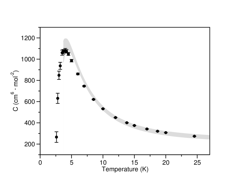
Figure 1: The third virial coefficient of ⁴He. The black circles are the results of the present calculations, with error bars representing expanded uncertainties with coverage factor $k=2$. The gray area shows the results of the recent low-temperature experiments by Gaiser and collaborators. Gaiser and Fellmuth (2009); Gaiser, Fellmuth, and Haft (2010)

We report in Table 1 the values of the third virial coefficient of ⁴He, together with the various contributions of Eq. (22), for temperatures in the range from $2.6$ K to $24.5561$ K, which is the lowest temperature studied in our previous work. Garberoglio and Harvey (2009) The same data are plotted in Figure 1, where they are compared with the recent experimental measurements by Gaiser and collaborators. Gaiser and Fellmuth (2009); Gaiser, Fellmuth, and Haft (2010)

More extensive comparison with available data over a wide range of temperatures will be presented elsewhere. Garberoglio, Moldover, and Harvey (tion) In Fig. 1, our results are plotted with expanded uncertainties with coverage factor $k=2$ as derived in Ref. Garberoglio, Moldover, and Harvey, tion; the uncertainty at the same expanded level for the experimental results was estimated from a figure in Ref. Gaiser and Fellmuth, 2009.

First, we notice that exchange effects are completely negligible in the calculation of the third virial coefficient for temperatures larger than 7 K, where their contribution to the overall value is close to one thousandth of that of the Boltzmann part. This is analogous to what has already been observed for the second virial coefficient.

When the temperature is lower than 7 K, the various exchange terms have contributions of similar magnitude and opposite sign, but their overall contribution to $C(T)$ is positive at all the temperatures that have been investigated. The exchange contribution to $C(T)$ is comparable to the statistical uncertainty of the calculation, which progressively increases as the temperature is lowered.

In Fig. 1, it can be seen that our theoretical values of $C(T)$ are compatible with those of recent experiments Gaiser and Fellmuth (2009); Gaiser, Fellmuth, and Haft (2010) down to the temperature of 10 K. For lower temperatures, the experimental results are somewhat larger than the calculated values, even though agreement is found again for temperatures below 4 K, where $C(T)$ passes through a maximum.

III.3 The third virial coefficient of ³He

Similar behavior is observed in the case of the third virial coefficient for ³He, whose calculated values are reported in Table 2. Also in this case the exchange contributions are of opposite signs, but their combined effect is to reduce the value obtained with Boltzmann statistics, which is the opposite trend to that observed for ⁴He.

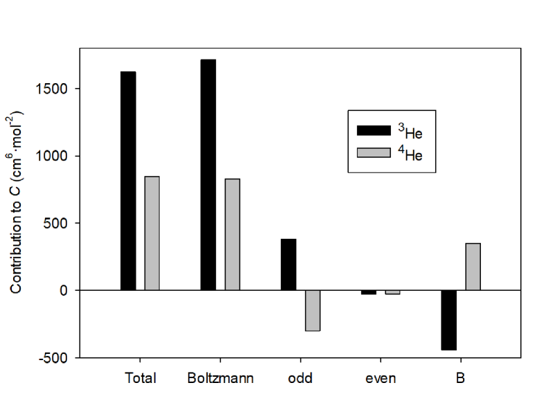
Figure 2: The magnitude and sign of the various contributions to $C(T)$ at $T=3$ K.

The effects of the various contributions to the third virial coefficient, in both the Bose–Einstein and Fermi–Dirac case, are summarized in Fig. 2 for the representative temperature of $T=3$ K. First, we notice that the largest contribution to the third virial coefficient comes from the Boltzmann term. The even exchange term has only a minor contribution, whereas the two remaining terms ($C_{\mathrm{odd}}$ and $C_{\mathrm{B}}$) have almost equal magnitudes and opposite signs. In the case of Bose–Einstein statistics, the contribution to $C$ from $C_{\mathrm{odd}}$ is negative, while that from $C_{\mathrm{B}}$ is positive; the opposite situation is observed in the case of Fermi–Dirac statistics. The overall sum of the exchange contributions is positive for ⁴He and negative in the case of ³He.

The magnitude of each exchange contribution at a given temperature is significantly greater for ³He; this reflects the larger de Broglie wavelength, which not only appears directly in the exchange terms but also affects the range of space sampled by the ring polymers.

In the case of ³He, the exchange contribution is significantly larger than the uncertainty of our calculations, at least at the lowest temperatures that we have investigated. Similarly to the case of ⁴He, quantum statistical effects on $C(T)$ contribute less than one part in a thousand for temperatures higher than 7 K. Even in the case of ³He, we observe $C(T)$ pass through a maximum, at a temperature around 3 K, which is 1 K lower than the temperature where $C(T)$ reaches a maximum for the ⁴He isotope.

Temperature	$C$		$C_{\mathrm{Boltzmann}}$		$C_{\mathrm{odd}}$		$C_{\mathrm{even}}$		$C_{\mathrm{B}}$
$(\mathrm{K})$	$(\mathrm{cm}^{6}~{}\mathrm{mol}^{-2})$		$(\mathrm{cm}^{6}~{}\mathrm{mol}^{-2})$		$(\mathrm{cm}^{6}~{}\mathrm{mol}^{-2})$		$(\mathrm{cm}^{6}~{}\mathrm{mol}^{-2})$		$(\mathrm{cm}^{6}~{}\mathrm{mol}^{-2})$
$2.6$	$1657$	$\pm 29$	$1857$	$\pm 28$	$-1803$	$\pm 4$	$-274.8$	$\pm 0.8$	$-1033$	$\pm 5$
$2.8$	$1686$	$\pm 23$	$1817$	$\pm 23$	$-1164$	$\pm 3$	$-167.9$	$\pm 0.6$	$-671$	$\pm 4$
$3$	$1622$	$\pm 17$	$1712$	$\pm 17$	$-760.2$	$\pm 2.2$	$-105.7$	$\pm 0.4$	$-443.3$	$\pm 2.2$
$3.2$	$1561$	$\pm 17$	$1621$	$\pm 17$	$-503.5$	$\pm 1.7$	$-66.8$	$\pm 0.3$	$-295$	$\pm 1.6$
$3.5$	$1451$	$\pm 13$	$1487$	$\pm 13$	$-277.2$	$\pm 1.2$	$-34.89$	$\pm 0.15$	$-165.8$	$\pm 1.1$
$3.7$	$1412$	$\pm 11$	$1439$	$\pm 11$	$-189.2$	$\pm 0.8$	$-23.12$	$\pm 0.11$	$-115.5$	$\pm 1$
$4$	$1326$	$\pm 9$	$1342$	$\pm 9$	$-107$	$\pm 0.5$	$-12.69$	$\pm 0.07$	$-66.5$	$\pm 0.7$
$4.2$	$1261$	$\pm 9$	$1273$	$\pm 9$	$-73.9$	$\pm 0.5$	$-8.65$	$\pm 0.05$	$-46.8$	$\pm 0.2$
$4.5$	$1183$	$\pm 7$	$1190$	$\pm 7$	$-43.7$	$\pm 0.3$	$-4.86$	$\pm 0.03$	$-27.9$	$\pm 0.2$
$5$	$1075$	$\pm 6$	$1079$	$\pm 6$	$-18.41$	$\pm 0.16$	$-1.963$	$\pm 0.016$	$-12.31$	$\pm 0.13$
$6$	$896$	$\pm 4$	$897$	$\pm 4$	$-3.56$	$\pm 0.06$	$-0.353$	$\pm 0.005$	$-2.52$	$\pm 0.04$
$7$	$773$	$\pm 3$	$773$	$\pm 3$	$-0.78$	$\pm 0.02$	$-0.0784$	$\pm 0.002$	$-0.6$	$\pm 0.01$
$8.5$	$645$	$\pm 2$	$645$	$\pm 2$	$-0.059$	$\pm 0.006$	$-0.0087$	$\pm 0.0003$	$-0.072$	$\pm 0.003$
$10$	$558.3$	$\pm 1.6$	$558.3$	$\pm 1.6$
$12$	$475.5$	$\pm 1.1$	$475.5$	$\pm 1.1$
$13.8033$	$426.2$	$\pm 0.8$	$426.2$	$\pm 0.8$
$15$	$402.0$	$\pm 0.7$	$402.0$	$\pm 0.7$
$17$	$369.6$	$\pm 0.5$	$369.6$	$\pm 0.5$
$18.689$	$347.8$	$\pm 0.4$	$347.8$	$\pm 0.4$
$20$	$333.4$	$\pm 0.4$	$333.4$	$\pm 0.4$
$24.5561$	$297.8$	$\pm 0.3$	$297.8$	$\pm 0.3$

Table 2: Values of the third virial coefficient of ³He and its components at selected temperatures. Note that the various contributions should be summed with the weights appearing in Eq. (22) with $I=1/2$. The $\pm$ values reflect only the standard uncertainty of the Monte Carlo integration; see Ref. Garberoglio, Moldover, and Harvey, tion for complete uncertainty analysis.

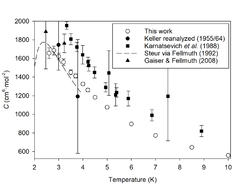
Figure 3: The third virial coefficient of ³He.

There are only a few sources of experimental data for $C(T)$ for ³He. Keller Keller (1955) measured five pressure-volume isotherms at temperatures below 4 K; these were later reanalyzed by Roberts et al. Roberts, Sherman, and Sydoriak (1964) and meaningful values of $C$ were obtained only for the two highest temperatures. A later analysis of the Keller data was performed by Steur (unpublished), whose equation for temperatures below 3.8 K was reported by Fellmuth and Schuster Fellmuth and Schuster (1992). Some points were also extracted from volumetric data by Karnatsevich et al. Karnatsevich, Bogoyavlenskii, and Titar (1988) Recently, Gaiser and Fellmuth Gaiser and Fellmuth (2008); Gaiser extracted virial coefficients from their measurements of two isotherms for ³He with dielectric-constant gas thermometry.

Figure 3 compares our calculated values to the available experimental data, where the error bars represent expanded uncertainties with coverage factor $k=2$. Error bars are not drawn for our values above 5 K because they would be smaller than the size of the symbol. As was the case in our previous work, Garberoglio and Harvey (2009) the uncertainty of our values of $C(T)$ is determined by the statistical uncertainty of our Monte Carlo calculations (shown in Tables 1 and 2) and by the uncertainty in the two- and three-body potentials. At the temperatures considered here, the statistical uncertainty is the dominant contribution to the overall uncertainty. The full uncertainty analysis is presented elsewhere. Garberoglio, Moldover, and Harvey (tion)

For the experimental points, these expanded uncertainties were taken as reported in the original sources; we note that in some cases (notably Ref. Karnatsevich, Bogoyavlenskii, and Titar, 1988) this appears to be merely the scatter of a fit and therefore underestimates the total uncertainty.

Our results are qualitatively similar to the rather scattered experimental data. We are quantitatively consistent with the values based on analysis of the data of Keller, but values from the other experimental sources are more positive than our results. We note that a similar comparison for ⁴He Garberoglio, Moldover, and Harvey (tion), where the experimental data situation is much better, shows the $C(T)$ values of Ref. Karnatsevich, Bogoyavlenskii, and Titar, 1988 for ⁴He to deviate in a very similar way not only from our results but from other experimental data we consider to be reliable.

IV Conclusions

We used path-integral methods to derive an expression for the third virial coefficient of monatomic gases, including the effect of quantum statistics. We applied this formalism to the case of helium isotopes, using state-of-the-art two- and three-body potentials.

We showed that exchange effects make no significant contribution to the third virial coefficient above a temperature of approximately 7 K for both the fermionic and bosonic isotope. This is the same behavior observed in the calculation of the second virial coefficient. For temperatures lower than $7$ K, the sign of the contribution to $C(T)$ from exchange effects depends on the bosonic or fermionic nature of the atom. In the case of ⁴He, the exchange contribution to $C(T)$ increases its value compared to the value obtained with Boltzmann statistics, although in our simulations the total exchange contribution has the same order of magnitude as the statistical uncertainty of the PIMC integration. In the case of ³He, the exchange contribution is negative, and its magnitude is much larger than the statistical uncertainty.

The range of temperatures that we have investigated covers the low-temperature maximum of $C(T)$ for both isotopes. The third virial coefficient of ⁴He reaches its maximum close to $4$ K, whereas in the case of ³He the maximum is attained at a lower temperature.

For both helium isotopes, the uncertainty in our calculated third virial coefficients is much smaller than that of the limited and sometimes inconsistent experimental data. For ⁴He, we obtain good agreement with the most recent experimental results, except for some temperatures below 10 K. A full comparison with available experimental data for ⁴He, including the higher temperatures of importance for metrology, will be presented elsewhere.Garberoglio, Moldover, and Harvey (tion) For ³He, we are qualitatively consistent with the sparse and scattered experimental values; in this case especially our calculations provide results that are much less uncertain than experiment. In both cases, at the temperatures considered here, the uncertainty is dominated by the statistical uncertainty of the Monte Carlo integration, meaning that the uncertainty of $C(T)$ could be reduced somewhat with greater expenditure of computer resources.

We note two directions in which extension of the present work could be fruitful. One is the calculation of higher-order virial coefficients, which is a straightforward extension of the method presented here. This would be much more computationally demanding, but the fourth virial coefficient $D(T)$ may be feasible, at least at higher temperatures where the number of beads in the ring polymers would not be large. Second, the method can be extended to calculate temperature derivatives such as $\mathrm{d}C/\mathrm{d}T$; such derivatives are of interest in interpreting acoustic measurements. Work on the evaluation of acoustic virial coefficients is in progress. Garberoglio, Moldover, and Harvey (tion)