Langevin process reflected on a partially elastic boundary II

Laboratoire de Probabilités et Modèles Aléatoires
Université Pierre et Marie Curie
4 place Jussieu, 75005 Paris, France

Abstract

A particle subject to a white noise external forcing moves like a Langevin process. Consider now that the particle is reflected at a boundary which restores a portion $c$ of the incoming speed at each bounce. For $c$ strictly smaller than the critical value $c_{crit}=\exp(-\pi/\sqrt{3})$, the bounces of the reflected process accumulate in a finite time. We show that nonetheless the particle is not necessarily absorbed after this time. We define a “resurrected” reflected process as a recurrent extension of the absorbed process, and study some of its properties. We also prove that this resurrected reflected process is the unique solution to the stochastic partial differential equation describing the model. Our approach consists in defining the process conditioned on never being absorbed, via an $h-$transform, and then giving the Itō excursion measure of the recurrent extension thanks to a formula fairly similar to Imhof’s relation.

Key words. Langevin process, second order reflection, recurrent extension, excursion measure, stochastic partial differential equation, $h$-transform.

A.M.S classification. (MSC2010) 60J50, 60H15

1 Introduction

Consider a particle in a one-dimensional space, submitted to a white noise external forcing. Its velocity is then well-defined and given by a Brownian motion, while its position is given by a so-called Langevin process. The Langevin process is non-Markov, therefore its study is often based on that of the Kolmogorov process, which is Markov. This Kolmogorov process is simply the two-dimensional process, whose first coordinate is a Langevin process, and second coordinate its derivative. We refer to Lachal [12] for a detailed account about it. Further, suppose that the particle is constrained to stay in $[0,+\infty[$ by a boundary at 0 characterized by an elasticity coefficient $c\geq 0$. That is, the boundary restores a portion $c$ of the incoming velocity at each bounce, and the equation of motion that we consider is the following:

$$(SOR)\qquad\left\{\begin{array}[]{ccl}X_{t}&=&X_{0}+\displaystyle\int_{0}^{t}\dot{X}_{s}\mathrm{d}s\\ \\ \dot{X}_{t}&=&\dot{X}_{0}+B_{t}-(1+c)\sum_{0<s\leq t}\dot{X}_{s-}\mathbbm{1}_{X_{s}=0},\end{array}\right.$$

where $B$ is a standard Brownian motion and $(X_{0},\dot{X}_{0})$ is called the initial or starting condition. This stochastic partial differential equation is nice outside the point $(0,0)$. Indeed, if the starting condition is different from $(0,0)$, there is a simple pathwise construction of the solution to this equation system, until time $\zeta_{\infty}$, the hitting time of $(0,0)$ for the process $(X,\dot{X})$. However there is a tough problem at $(0,0)$. Indeed, there exists an old literature about a deterministic analogue to theses equations, where the white noise force is replaced by a deterministic force. See Ballard [1] for a vast review. As early as in 1960, Bressan [6] pointed out that multiple solutions may occur, even when the force is $\mathcal{C}^{\infty}$. It appears that the introduction of a white noise allows to get back a weak uniqueness result. We refer to [4] (see also [3], [11]) for the particular case $c=0$.

In [10], we have shown for $c>0$ the existence of two different regimes, the critical elasticity being $c_{crit}:=\exp(-\pi/\sqrt{3})$. It is critical in the sense that when the starting condition is different from $(0,0)$, then we have $\zeta_{\infty}=+\infty$ almost surely if $c\geq c_{crit}$, and $\zeta_{\infty}<+\infty$ almost surely if $c<c_{crit}$. Further, we studied the super-critical and the critical regimes. In this paper, we study the sub-critical regime $c<c_{crit}$. The finite time $\zeta_{\infty}$ corresponds to an accumulation of bounces in a finite time. We write $\mathbb{P}_{x,u}^{c}$ for the law of the reflected Kolmogorov process, with starting condition $(x,u)\neq(0,0)$, elasticity coefficient $c$, and killed at time $\zeta_{\infty}$. It is the unique strong solution to $(SOR)$ equations, up to time $\zeta_{\infty}$. We also write $\mathrm{P}_{t}^{c}$ for the associated semigroup. We will devote ourselves to prove the existence of a unique recurrent extension to this process that leaves $(0,0)$ continuously. Moreover, we will prove that this extension gives the unique solution, in the weak sense, to $(SOR)$ equations.

We point out that this model was encountered by Bect in his thesis ([2], section III.4.B). He observed the existence of the critical elasticity and asked several questions on the different regimes. We answer to all of them.

In this work we will be largely inspired by a paper of Rivero [15], in which he studies the recurrent extensions of a self-similar Markov process with semigroup $\mathrm{P}_{t}$. Briefly, first, he recalls that recurrent extensions are equivalent to excursion measures compatible with $\mathrm{P}_{t}$, thanks to Itō’s program. Then a change of probability allows him to define the Markov process conditioned on never hitting $0$, where this conditioning is in the sense of Doob, via an $h-$transform. An inverse $h-$transform on the Markov process conditioned on never hitting zero and starting from 0 then gives the construction of the excursion measure.

We will not recall it at each step throughout the paper, but a lot of parallels can be made. However, it is a two-dimensional Markov process that we consider here. Further, its study will rely on an underlying random walk $(S_{n})_{n\in\mathbb{N}}$ constructed from the velocities at bouncing times.

In the Preliminaries, we introduce this random walk and use it to estimate the tail of the variable $\zeta_{\infty}$ under $\mathbb{P}_{0,1}^{c}$. In the Section 3, we introduce a change of probability, via an $h-$transform, to define $\widetilde{\mathbb{P}}_{x,u}$, law of a process which can be viewed as the reflected Kolmogorov process conditioned on never being killed. We then show in Subsection 3.2 that this law has a weak limit $\widetilde{\mathbb{P}}_{0^{+}}$ when $(x,u)$ goes to $(0,0)$, using the same method that was used in [10] to show that for $c>c_{crit}$, the laws $\mathbb{P}_{0,u}^{c}$ have the weak limit $\mathbb{P}_{0+}^{c}$ when $u$ goes to zero. All this section can be seen as a long digression to prepare the construction of the excursion measure in Section 4. This excursion measure is defined by a formula similar to Imhof’s relation (see [9]), connecting the excursion measure of Brownian motion and the law of a Bessel(3) process. But our formula involves the law $\mathbb{P}_{0+}^{c}$ and determines the unique excursion measure compatible with the semigroup $\mathrm{P}_{t}^{c}$ . We call resurrected Kolmogorov process the corresponding recurrent extension. Finally, we prove that this is the (weakly) unique solution to $(SOR)$ equations when the starting condition is $(0,0)$.

2 Preliminaries

We largely use the same notations as in [10]. For the sake of simplicity, we use the same notation (say $P$) for a probability measure and for the expectation under this measure. We will even authorize ourselves to write $P(f,A)$ for the quantity $P(f\mathbbm{1}_{A})$, when $f$ is a measurable functional and $A$ an event. We introduce $D=(\{0\}\times\mathbb{R}_{+}^{*})\cup(\mathbb{R}_{+}^{*}\times\mathbb{R})$ and $D^{0}:=D\cup\{(0,0)\}$. Our working space is $\mathcal{C}$, the space of càdlàg trajectories $(x,\dot{x}):[0,\infty)\to D^{0}$, which satisfy

$$x(t)=x(0)+\displaystyle\int_{0}^{t}\dot{x}(s)\mathrm{d}s.$$

That space is endowed with the $\sigma-$algebra generated by the coordinate maps and with the topology induced by the following injection:

$$\begin{array}[]{ccc}\mathcal{C}&\to&\mathbb{R}_{+}\times\mathbb{D}\\ (x,\dot{x})&\mapsto&\big{(}x(0),\dot{x}\big{)},\end{array}$$

where $\mathbb{D}$ is the space of càdlàg trajectories on $\mathbb{R}_{+}$, equipped with Skorohod topology.

We denote by $(X,\dot{X})$ the canonical process and by $(\mathfrak{F}_{t},t\geq 0)$ its natural filtration, satisfying the usual conditions of right continuity and completeness. For an initial condition $(x,u)\in D$, the $(SOR)$ equations

$$\left\{\begin{array}[]{ccl}X_{t}&=&x+\displaystyle\int_{0}^{t}\dot{X}_{s}\mathrm{d}s\\ \\ \dot{X}_{t}&=&u+B_{t}-(1+c)\sum_{0<s\leq t}\dot{X}_{s-}\mathbbm{1}_{X_{s}=0}\end{array}\right.$$

have a unique solution, at least up to the random time

$$\zeta_{\infty}:=\inf\{t>0,X_{t}=0,\dot{X}_{t}=0\}.$$

We call (killed) reflected Kolmogorov process this solution killed at time $\zeta_{\infty}$, and write $\mathbb{P}_{x,u}^{c}$ for its law. It is Markov. We also call reflected Langevin process the first coordinate of this process, which is no longer Markov.

Call $\zeta_{1}$ the first hitting time of zero for the reflected Langevin process $X$, that is $\zeta_{1}:=\inf\{t>0,X_{t}=0\}$. More generally, the sequence of the successive hitting times of zero $(\zeta_{n})_{n\geq 1}$ is defined recursively by $\zeta_{n+1}:=\inf\{t>\zeta_{n},X_{t}=0\}$. We write $(V_{n})_{n\geq 1}:=(\dot{X}_{\zeta_{n}})_{n\geq 1}$ for the sequence of the velocities of the process at these hitting times. That means outgoing velocities, as we are dealing with right-continuous processes. Finally, when the starting position is $x=0$, we will simply write $\mathbb{P}^{c}_{u}$ for $\mathbb{P}^{c}_{0,u}$, and we will also define $\zeta_{0}=0$ and $V_{0}=\dot{X}_{0}$. We insist on the fact that in each case the starting condition $(x,u)$ is different from $(0,0)$. Then it is not difficult to see that $\zeta_{\infty}$ coincides almost surely with $\sup\zeta_{n}$. But we can say much more.

The sequence $\left(\dfrac{\zeta_{n+1}-\zeta_{n}}{V_{n}^{2}},\dfrac{V_{n+1}}{V_{n}}\right)_{n\geq 0}$ is i.i.d. and of law independent of $u$, which can be deduced from the following density:

$$\frac{1}{\mathrm{d}s\mathrm{d}v}\mathbb{P}_{1}^{c}\left(({\zeta_{1}},{V_{1}}/c)\in(\mathrm{d}s,\mathrm{d}v)\right)=\frac{3v}{\pi\sqrt{2}s^{2}}\exp(-2\frac{v^{2}-v+1}{s})\int_{0}^{4v/s}e^{-\frac{3\theta}{2}}\frac{\mathrm{d}\theta}{\sqrt{\pi\theta}},$$ (2.1)

given by McKean [13]. The second marginal of this density is

$$\mathbb{P}_{1}^{c}({V_{1}}/c\in\mathrm{d}v)=\frac{3}{2\pi}\frac{v^{\frac{3}{2}}}{1+v^{3}}\mathrm{d}v.$$ (2.2)

In particular, the sequence $S_{n}:=\ln(V_{n})$ is a random walk, with drift

$$\mathbb{P}_{1}^{c}(S_{1}-S_{0})=\ln(c)+\frac{\pi}{\sqrt{3}},$$

which is zero for the critical value $c_{crit}=\exp(-\pi/\sqrt{3})$. In this paper we lie in the subcritical case $c<c_{crit}$, when the drift is negative. A thorough study allows to not only deduce the finiteness of $\zeta_{\infty}$, but also estimate its tail.

Lemma 1.

We have

$$\mathbb{P}_{1}^{c}\left(V_{1}^{x}\right)=\frac{c^{x}}{2\cos(\frac{x+1}{3}\pi)}\textrm{ for }x<1/2.$$ (2.3)

There exists a unique $k=k(c)$ in $(0,1/4)$ such that $\mathbb{P}_{1}^{c}\left(V_{1}^{2k}\right)=1$, and

$$\mathbb{P}_{1}^{c}(\zeta_{\infty}>t)\underset{t\to\infty}{\sim}C_{1}t^{-k},$$ (2.4)

where $C_{1}=C_{1}(c)\in(0,\infty)$ is a constant depending only on $c$, given by

$$C_{1}=\frac{\mathbb{P}_{1}^{c}\left(\zeta_{\infty}^{k}-(\zeta_{\infty}-\zeta_{1})^{k}\right)}{k\mathbb{P}_{1}^{c}(V_{1}^{2k}\ln(V_{1}^{2}))}.$$ (2.5)

In other words, $k(c)$ is given implicitly as the unique solution in $]0,\frac{1}{4}]$ of the equation

$$c=\left[2\cos\left(\frac{2k+1}{3}\pi\right)\right]^{\frac{1}{2k}}.$$ (2.6)

The upper bound $1/4$ stems from the fact that $\mathbb{P}_{1}^{c}\left(V_{1}^{2k}\right)$ becomes infinite for $k=1/4$. The value of $k(c)$ converges to $1/4$ when $c$ goes to 0, and to $0$ when $c$ goes to $c_{crit}$, as illustrated by Figure 1. We may notice that Formula (2.4) remains true for $c=0$ and $k=1/4$ (and for $c=c_{crit}$ and $k=0$, in a certain sense).

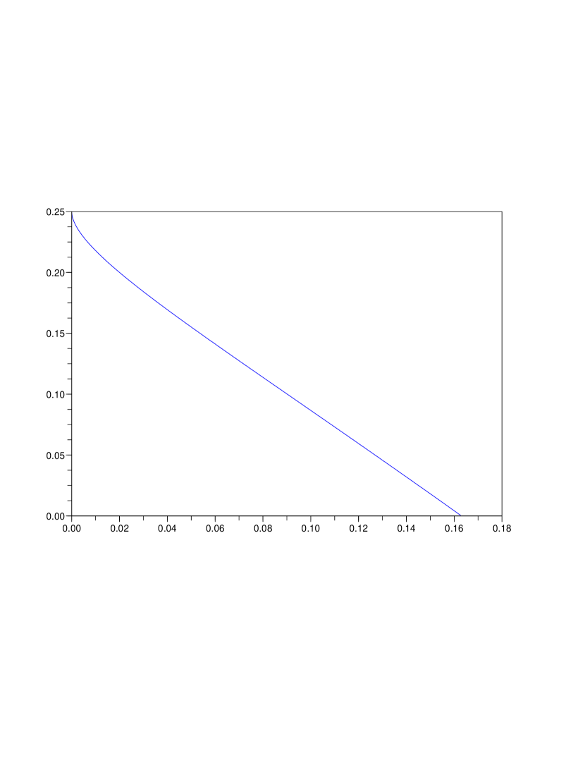
Figure 1: Graph of the exponent k(c)

Proof.

Formula (2.3) is not new. For the convenience of the reader, we still provide the following calculation. From Formula (2.2), it follows, for $x<1/2$,

$$\mathbb{P}_{1}^{c}\left(\left({V_{1}}/c\right)^{x}\right) = \frac{3}{2\pi}\int_{0}^{\infty}\frac{t^{x+3/2}}{1+t^{3}}\mathrm{d}t=\frac{1}{2\pi}\int_{0}^{\infty}\frac{t^{\frac{x}{3}-\frac{1}{6}}}{1+t}\mathrm{d}t.$$

Note $\cos(\frac{x+1}{3}\pi)=\sin(\pi y)$, where $y=\frac{x}{3}+\frac{5}{6}$. Using the variable $y$, which belongs to $(0,1)$, Equation (2.3) becomes

$$\int_{0}^{\infty}\frac{t^{y-1}}{1+t}\mathrm{d}t=\frac{\pi}{\sin(\pi y)},$$

and follows from:

$$\int_{0}^{\infty}\frac{t^{y-1}}{1+t}\mathrm{d}t = \int_{0}^{1}t^{y}(1-t)^{1-y}\mathrm{d}t$$

$$= \mathrm{B}(y,1-y)$$

$$= \frac{\Gamma(y)\Gamma(1-y)}{\Gamma(1)}$$

$$= \frac{\pi}{\sin(\pi y)}.$$

where $\mathrm{B}$ and $\Gamma$ are the usual Beta and Gamma function, respectively.

Now, the function $x\mapsto\mathbb{P}_{1}^{c}\left(V_{1}^{x}\right)$ is convex, takes value 1 at $x=0$ and becomes infinite at $x=1/2$. Its derivative at 0 is equal to $\mathbb{P}_{1}^{c}(S_{1}-S_{0})<0.$ We deduce that there is indeed a unique $k(c)$ in $(0,\frac{1}{4})$ such that $\mathbb{P}_{1}^{c}\left(V_{1}^{2k}\right)=1.$

Estimate (2.4) will appear as a particular case of an “implicit renewal theory” result of Goldie [7]. Let us express $\zeta_{\infty}$ as the series:

$$\zeta_{\infty} = \sum_{n=1}^{\infty}\frac{\zeta_{n}-\zeta_{n-1}}{V_{n-1}^{2}}V_{n-1}^{2},$$

with $V_{n}^{2}:=V_{1}^{2}\frac{V_{2}^{2}}{V_{1}^{2}}\cdot\cdot\cdot\frac{V_{n}^{2}}{V_{n-1}^{2}}$, and where $\left(\dfrac{\zeta_{n}-\zeta_{n-1}}{V_{n-1}^{2}},\dfrac{V_{n}^{2}}{V_{n-1}^{2}}\right)_{n\geq 1}$ is i.i.d. We lie in the setting of Section 4 of Goldie’s paper [7], and can apply its Theorem (4.1). Indeed, all the following conditions are satisfied:

$$\mathbb{P}_{1}^{c}(V_{1}^{2k})=1,$$

$$\mathbb{P}_{1}^{c}(V_{1}^{2k}\ln(V_{1}^{2}))<\infty,$$

$$\mathbb{P}_{1}^{c}(\zeta_{1}^{k})<\infty,$$

the last one being a consequence of the inequality $k<1/4$ and of the following estimate of the queue of the variable $\zeta_{1}$,

$$\mathbb{P}_{1}^{c}(\zeta_{1}>t)\underset{t\to\infty}{\sim}c^{\prime}t^{-\frac{1}{4}},$$ (2.7)

which was already pointed out in Lemma 1 in [10]. All this is enough to apply the theorem of Goldie and deduce the requested result, namely

$$\mathbb{P}_{1}^{c}(\zeta_{\infty}>t)\underset{t\to\infty}{\sim}C_{1}t^{-k},$$

where $C_{1}$ is the constant defined by (2.5), and belongs to $]0,\infty[$. ∎

Next section is devoted to the definition and study of the reflected Kolmogorov process, conditioned on never hitting $(0,0)$. This process will be of great use for studying the recurrent extensions of the reflected Kolmogorov process in Section 4.

3 The reflected Kolmogorov process conditioned on never hitting $(0,0)$

3.1 Definition via an $h-$transform

Recall that under $\mathbb{P}_{1}^{c}$, the sequence $(S_{n})_{n\geq 0}=(\ln(V_{n}))_{n\geq 0}$ is a random walk starting from 0, and write $\mathbf{P}_{0}$ for its law. The important fact $\mathbb{P}_{1}^{c}(V_{1}^{2k})=1$ implies $\mathbb{P}_{1}^{c}(V_{n}^{2k})=1$ for any $n>0$, and can be rewritten $\mathbf{P}_{0}(\theta^{S_{n}})=1$, with $\theta:=\exp(2k)$.

The sequence $\theta^{S_{n}}$ being a martingale, we introduce the change of probability

$$\widetilde{\mathbf{P}}_{0}(S_{n}\in\mathrm{d}t)=\theta^{t}\mathbf{P}_{0}(S_{n}\in\mathrm{d}t).$$

Under $\widetilde{\mathbf{P}}_{0}$, $(S_{n})_{n\geq 0}$ becomes a random walk drifting to $+\infty$. Informally, it can be viewed as being the law of the random walk $S_{n}$ under $\mathbf{P}_{0}$ conditioned on hitting arbitrary high levels.

There is a corresponding change of probability for the reflected Kolmogorov process and its law $\mathbb{P}_{1}^{c}$. We introduce the law $\widetilde{\mathbb{P}}_{1}$ determined by

$$\widetilde{\mathbb{P}}_{1}(A\mathbbm{1}_{\zeta_{n}>T})=\mathbb{P}^{c}_{1}(A\mathbbm{1}_{\zeta_{n}>T}\mathbb{P}_{1}^{c}(V_{n}^{2k}|\mathfrak{F}_{T})),$$

for any $n>0$, stopping-time $T$ and $A\in\mathfrak{F}_{T}$. By the strong Markov property we have

$$\mathbb{P}_{1}^{c}(V_{n}^{2k}|\mathfrak{F}_{T})=\mathbb{P}_{X_{T},\dot{X}_{T}}^{c}(V_{1}^{2k})\qquad\text{on the event }\{\zeta_{n}>T\},$$

so that there is the identity

$$\widetilde{\mathbb{P}}_{1}(A\mathbbm{1}_{\zeta_{n}>T})=\mathbb{P}^{c}_{1}(A\mathbbm{1}_{\zeta_{n}>T}H(X_{T},\dot{X}_{T})),$$

where we have written

$$H(x,u):=\mathbb{P}_{x,u}^{c}(V_{1}^{2k}).$$

Note that $H(0,u)=u^{2k}$. Letting $n$ go to infinity, we get:

$$\widetilde{\mathbb{P}}_{1}(A\mathbbm{1}_{\zeta_{\infty}>T})=\mathbb{P}^{c}_{1}(A\mathbbm{1}_{\zeta_{\infty}>T}H(X_{T},\dot{X}_{T})).$$

We have $H(0,1)=1$, the function $H$ is harmonic for the semigroup of the reflected Kolmogorov process, and the process $\widetilde{\mathbb{P}}_{1}$ is the $h-$transform of $\mathbb{P}_{1}^{c}$, in the sense of Doob.

Under $\widetilde{\mathbb{P}}_{1}$, the law of the sequence $(S_{n})_{n\geq 0}$ is $\widetilde{\mathbf{P}}_{0}$, thus this sequence is diverging to $+\infty$, and as a consequence the time $\zeta_{\infty}$ is infinite $\widetilde{\mathbb{P}}_{1}-$almost surely. The term $\mathbbm{1}_{\zeta_{\infty}>T}$ in $\widetilde{\mathbb{P}}_{1}(A\mathbbm{1}_{\zeta_{\infty}>T})$ is thus unnecessary. We may now give a more general definition of this change of probability, as an $h-$transform, for any starting position $(x,u)$.

Definition 1.

The reflected Kolmogorov process conditioned on never hitting $(0,0)$ is the Markov process given by its law $\widetilde{\mathbb{P}}_{x,u}$, for any starting condition $(x,u)\in D$, which is the unique measure such that for every stopping-time $T$ we have

$$\widetilde{\mathbb{P}}_{x,u}(A)=\frac{1}{H(x,u)}\mathbb{P}_{x,u}^{c}(AH(X_{T},\dot{X}_{T}),T<\zeta_{\infty}),$$ (3.1)

for any $A\in\mathfrak{F}_{T}$. We write $\widetilde{\mathrm{P}}_{t}$ its associated semigroup, and we also write $\widetilde{\mathbb{P}}_{u}$ for $\widetilde{\mathbb{P}}_{0,u}$.

This denomination is justified by the following proposition.

Proposition 1.

For any $(x,u)\in D$ and $t>0$, we have

$$\widetilde{\mathbb{P}}_{x,u}(A)=\lim_{s\to\infty}\mathbb{P}^{c}_{x,u}(A|\zeta_{\infty}>s),$$ (3.2)

for any $A\in\mathfrak{F}_{t}$.

We stress that in [15], Proposition 2, Rivero defines in a similar way the self-similar Markov process conditioned on never hitting 0. Incidentally, you can find in [11] a thorough study of other $h-$transforms regarding the Kolmogorov process killed at time $\zeta_{1}$.

In order to get Formula (3.2), we first prove the following lemma, which is a slight improvement of (2.4):

Lemma 2.

For any $(x,u)\in D$,

$$s^{k}\mathbb{P}^{c}_{x,u}(\zeta_{\infty}>s)\underset{s\to\infty}{\longrightarrow}H(x,u)C_{1}.$$ (3.3)

Proof.

For $(x,u)=(0,1)$, this is (2.4). For $x=0$, the rescaling invariance property yields immediately

$$s^{k}\mathbb{P}^{c}_{0,u}(\zeta_{\infty}>s)=s^{k}\mathbb{P}^{c}_{0,1}(\zeta_{\infty}>su^{-2})\underset{s\to\infty}{\longrightarrow}u^{2k}C_{1}=H(0,u)C_{1}.$$

For $(x,u)\in D$, the Markov property at time $\zeta_{1}$ yields

$$s^{k}\mathbb{P}^{c}_{x,u}(\zeta_{\infty}>s) = \mathbb{P}^{c}_{x,u}(s^{k}\mathbb{P}^{c}_{0,V_{1}}(\zeta_{\infty}>s-\zeta_{1}))$$

$$\underset{s\to\infty}{\longrightarrow} \mathbb{P}^{c}_{x,u}(H(0,V_{1})C_{1})=H(x,u)C_{1},$$

where the convergence holds by dominated convergence. The lemma is proved. ∎

Formula (3.2) then results from:

$$\mathbb{P}^{c}_{x,u}(A|\zeta_{\infty}>s) = \frac{1}{\mathbb{P}^{c}_{x,u}(\zeta_{\infty}>s)}\mathbb{P}^{c}_{x,u}\left(A\mathbb{P}^{c}_{X_{t},\dot{X}_{t}}(\zeta_{\infty}>s-t),\zeta_{\infty}>t\right)$$

$$\underset{s\to\infty}{\longrightarrow} \frac{1}{H(x,u)}\mathbb{P}^{c}_{x,u}\left(AH(X_{T},\dot{X}_{T}),\zeta_{\infty}>t\right)$$

$$= \ \widetilde{\mathbb{P}}_{x,u}(A).$$

3.2 Starting the conditioned process from $(0,0)$

The study of the reflected Kolmogorov process conditioned on never hitting $(0,0)$ will happen to be very similar to that of the reflected Kolmogorov process in the supercritical case $c>c_{crit}$, done in [10]. Observe the following similarities between the laws $\widetilde{\mathbb{P}}_{u}$, and $\mathbb{P}^{c}_{u}$ when $c>c_{crit}$: the sequence $\left(\dfrac{\zeta_{n+1}-\zeta_{n}}{V_{n}^{2}},\dfrac{V_{n+1}}{V_{n}}\right)_{n\geq 0}$ is i.i.d., we know its law explicitly, and the sequence $S_{n}=\ln(V_{n})$ is a random walk with positive drift. It follows that a major part of [10] can be transcribed mutatis mutandis. In particular we will get a convergence result for the probabilities $\widetilde{\mathbb{P}}_{u}$ when $u$ goes to zero, similar to Theorem 1 of [10].

Under $\widetilde{\mathbb{P}}_{1}$, the sequence $(S_{n})_{n\geq 0}$ is a random walk of law $\widetilde{\mathbf{P}}_{0}$. Write $\mu$ for its drift, that is the expectation of its jump distribution, which is positive and finite. The associated strictly ascending ladder height process $(H_{n})_{n\geq 0}$, defined by $H_{k}=S_{n_{k}}$, where $n_{0}=0$ and $n_{k}=\inf\{n>n_{k-1},S_{n}>S_{n_{k-1}}\}$, is a random walk with positive jumps. Its jump distribution also has positive and finite expectation $\mu_{H}\geq\mu$. The measure

$$m(\mathrm{d}y):=\frac{1}{\mu_{H}}\widetilde{\mathbf{P}}_{0}(H_{1}>y)\mathrm{d}y.$$ (3.4)

is the “stationary law of the overshoot”, both for the random walks $(S_{n})_{n\geq 0}$ and $(H_{n})_{n\geq 0}$. The following proposition holds.

Proposition 2.

The family of probability measures $(\widetilde{\mathbb{P}}_{x,u})_{(x,u)\in D}$ on $\mathcal{C}$ has a weak limit when $(x,u)\to(0,0)$, which we denote by $\widetilde{\mathbb{P}}_{0^{+}}$. More precisely, write $\tau_{v}$ for the instant of the first bounce with speed greater than $v$, that is $\tau_{v}:=\inf\{t>0,X_{t}=0,\dot{X}_{t}>v\}.$ Then the law $\widetilde{\mathbb{P}}_{0^{+}}$ satisfies the following properties:

$$\begin{array}[]{ll}(*)&\left\{\begin{array}[]{l}\displaystyle\lim_{v\to 0^{+}}\tau_{v}=0\quad\text{almost surely}.\\ \text{For any }u,v>0\text{, and conditionally on }\dot{X}_{\tau_{v}}=u\text{, the process }\\ (X_{\tau_{v}+t},\dot{X}_{\tau_{v}+t})_{t\geq 0}\text{ is independent of }(X_{s},\dot{X}_{s})_{s<\tau_{v}}\text{ and has law }\widetilde{\mathbb{P}}_{u}.\end{array}\right.\\ \\ (**)&\text{For any }v>0,\text{ the law of }\ln(\dot{X}_{\tau_{v}}/v)\text{ is }m.\end{array}$$

In the proof of this proposition we can take $x=0$ and just prove the convergence result for the laws $\widetilde{\mathbb{P}}_{u}$ when $u\to 0+$. The general result will follow as an application of the Markov property at time $\zeta_{1}$.

The complete proof follows mainly the proof of Theorem 1 in [10] and takes many pages. Here, the reader has three choices. Skip this proof and go directly to next section about the resurrected process. Or read the following for an overview of the ideas of the proof, with details given only when significantly different from that in [10]. Or, read [10] and the following, if (s)he wants to get the complete proof.

Call $T_{y}(S)$ the hitting time of $(y,\infty)$ for the random walk $S$ starting from $x<y$. Call $\widetilde{\mathbf{P}}_{\mu}$ the law of $(S_{n})_{n\geq 0}$ obtained by taking $S_{0}$ and $(S_{n}-S_{0})_{n\geq 0}$ independent, with law $m$ and $\widetilde{\mathbf{P}}_{0}$, respectively. That is, we allow the starting position to be nonconstant and distributed according to $\mu$. A result of renewal theory states that the law of the overshoot $(S_{n+T_{y}}-y)_{n\geq 0}$ under $\widetilde{\mathbf{P}}_{x}$, when $x$ goes to $-\infty$, converges to $\widetilde{\mathbf{P}}_{m}$. Now, for a process indexed by $I$ an interval of $\mathbb{Z}$, we define a spatial translation operator by $\Theta^{sp}_{y}((S_{n})_{n\in I})=(S_{n+T_{y}}-y)_{n\in{I-T_{y}}}$. We get that under $\widetilde{\mathbf{P}}_{x}$ and when $x$ goes to $-\infty$, the translated process $\Theta^{sp}_{y}(S)$ converges to a process called the “spatially stationary random walk", a process indexed by $\mathbb{Z}$ which is spatially stationary and whose restriction to $\mathbb{N}$ is $\widetilde{\mathbf{P}}_{m}$ (see [10]). We write $\widetilde{\mathbf{P}}$ for the law of this spatially stationary random walk.

There exists a link between the law $\widetilde{\mathbf{P}}_{x}$ and the law $\widetilde{\mathbb{P}}_{e^{x}}$: the first one is the law of the underlying random walk $(S_{n})_{n\geq 0}=(\ln V_{n})_{n\geq 0}$ for a process $(X,\dot{X})$ following the second one. Now, in a very brief shortcut, we can say that the law $\widetilde{\mathbf{P}}$ is linked to a law written $\widetilde{\mathbb{P}}_{0^{+}}^{*}$. And the convergence results of $\widetilde{\mathbf{P}}_{x}\circ\Theta^{sp}_{y}$ to $\mathbf{P}$ when $x\to-\infty$ provide convergence results of $\widetilde{\mathbb{P}}_{u}$ to $\widetilde{\mathbb{P}}_{0^{+}}^{*}$ when $u\to 0$.

However, this link is different, as the spatially stationary random walk, of law $\widetilde{\mathbf{P}}$, is a process indexed by $\mathbb{Z}$. The value $S_{0}$ is thus not equal to the logarithm of the velocity of the process at time 0, but at time $\tau_{1}$ (recall that $\tau_{1}=\inf\{t>0,X_{t}=0,\dot{X}_{t}\geq 1\}$ is the instant of the first bounce with speed no less than one). The sequence $(S_{n})_{n\geq 0}$ is then the sequence of the logarithms of the velocities of the process at the bouncing times, starting from that bounce. The sequence $(S_{-n})_{n\geq 0}$ is the sequence of the logarithms of the velocities of the process at the bouncing times happening before that bounce.

The law $\widetilde{\mathbb{P}}_{0^{+}}^{*}$ is the law of a process indexed by $\mathbb{R}_{+}^{*}$, but we actually construct it “from the random time $\tau_{1}$”. In order for the definition to be clean, we have to prove that the random time $\tau_{1}$ is finite a.s. In [10], we used the fact that if $(\zeta_{1,k})_{k\geq 0}$ is a sequence of i.i.d random variables, with common law that of $\zeta_{1}$ under $\mathbb{P}^{c}_{1}$, then for any $\varepsilon>0$ there is almost surely only a finite number of indexes $k$ such that $\ln(\zeta_{1,k})\geq\varepsilon k.$ This was based on Formula 2.7, which, we recall, states

$$\mathbb{P}_{1}^{c}(\zeta_{1}>t)\underset{t\to\infty}{\sim}c^{\prime}t^{-\frac{1}{4}},$$

where $c^{\prime}$ is some positive constant. Here the same results holds with replacing $\mathbb{P}^{c}_{1}$ by $\widetilde{\mathbb{P}}_{1}$ and is a consequence from the following lemma.

Lemma 3.

We have

$$\widetilde{\mathbb{P}}_{1}(\zeta_{1}>t)\underset{t\to\infty}{\sim}c^{\prime}t^{k-\frac{1}{4}},$$ (3.5)

where $c^{\prime}$ is some positive constant.

Proof.

From (3.1) and (2.1), we get that the density of $(\zeta_{1},V_{1}/c)$ under $\widetilde{\mathbb{P}}_{1}$ is given by

$$f(s,v):=\frac{1}{\mathrm{d}s\mathrm{d}v}\widetilde{\mathbb{P}}_{1}((\zeta_{1},V_{1}/c)\in\mathrm{d}s\mathrm{d}v) = (cv)^{2k}\frac{3v}{\pi\sqrt{2}s^{2}}\exp(-2\frac{v^{2}-v+1}{s})\int_{0}^{\frac{4v}{s}}e^{-\frac{3\theta}{2}}\frac{\mathrm{d}\theta}{\sqrt{\pi\theta}}.$$

Thanks to the inequality

$$4\sqrt{\frac{v}{s\pi}}e^{-\frac{6v}{s}}\leq\int_{0}^{\frac{4v}{s}}e^{-\frac{3\theta}{2}}\frac{\mathrm{d}\theta}{\sqrt{\pi\theta}}\leq 4\sqrt{\frac{v}{s\pi}},$$

we may write

$$f(s,v) = (6\sqrt{2}.\pi^{-\frac{3}{2}}c^{2k})s^{-\frac{5}{2}}v^{\frac{3}{2}+2k}e^{-2\frac{v^{2}}{s}+\frac{v}{s}K(s,v)},$$

where $(s,v)\mapsto K(s,v)$ is continuous and bounded. The marginal density of $\zeta_{1}$ is thus given by

$$\frac{1}{\mathrm{d}s}\widetilde{\mathbb{P}}_{1}(\zeta_{1}\in\mathrm{d}s) = \int_{\mathbb{R}_{+}}f(s,v)\mathrm{d}v$$

$$= (3\sqrt{2}.\pi^{-\frac{3}{2}}c^{2k})s^{-\frac{5}{4}+k}\int_{\mathbb{R}_{+}}w^{\frac{1}{4}+k}e^{-2w+K(s,\sqrt{sw})\sqrt{w/s}}\mathrm{d}w$$

$$\underset{s\to\infty}{\sim} (3\sqrt{2}.\pi^{-\frac{3}{2}}c^{2k})s^{-\frac{5}{4}+k}\int_{\mathbb{R}_{+}}w^{\frac{1}{4}+k}e^{-2w}\mathrm{d}w,$$

where we used successively the change of variables $w=v^{2}/s$ and dominated convergence theorem. Just integrate this equivalence in the neighborhood of $+\infty$ to get

$$\widetilde{\mathbb{P}}_{1}(\zeta_{1}>t)\underset{t\to\infty}{\sim}c^{\prime}t^{k-\frac{1}{4}},$$

with the constant

$$c^{\prime}=\frac{3\sqrt{2}.\pi^{-\frac{3}{2}}c^{2k}}{\frac{1}{4}-k}\int_{\mathbb{R}_{+}}w^{\frac{1}{4}+k}e^{-2w}\mathrm{d}w=\frac{3c^{2k}}{\pi^{\frac{3}{2}}2^{\frac{3}{4}+k}}\cdot\frac{1+4k}{1-4k}\ \Gamma\left(\frac{1}{4}+k\right).$$

∎

For now, we have introduced $\widetilde{\mathbb{P}}_{0^{+}}^{*}$, law of a process $(X,\dot{X})$ indexed by $\mathbb{R}_{+}^{*}$. We keep on following the proof of [10]. First, we get that this law satisfies conditions $(*)$ and $(**)$, and that for any $v>0$, the joint law of $\tau_{v}$ and $(X_{\tau_{v}+t},\dot{X}_{\tau_{v}+t})_{t\geq 0}$ under $\widetilde{\mathbb{P}}_{u}$ converges to that under $\widetilde{\mathbb{P}}_{0^{+}}^{*}$. Then we establish Proposition 2 by controlling the behavior of the process just after time 0, through the two following lemmas:

Lemma 4.

Under $\widetilde{\mathbb{P}}_{0^{+}}^{*}$, we have almost surely $(X_{t},\dot{X}_{t})\underset{t\to 0}{\longrightarrow}(0,0).$

This lemma allows in particular to extend $\widetilde{\mathbb{P}}_{0^{+}}^{*}$ to $\mathbb{R}_{+}$. We call $\widetilde{\mathbb{P}}_{0^{+}}$ this extension. The second lemma is more technical and controls the behavior of the process on $[0,\tau_{v}[$ under $\widetilde{\mathbb{P}}_{u}$.

Lemma 5.

Write $M_{v}=\sup\{|\dot{X}_{t}|,t\in[0,\tau_{v}[\}$. Then,

$$\forall\varepsilon>0,\forall\delta>0,\exists v_{0}>0,\exists u_{0}>0,\forall 0<u\leq u_{0},\quad\widetilde{\mathbb{P}}_{u}(M_{v_{0}}\geq\delta)\leq\varepsilon,$$ (3.6)

In [10], we proved these two results by using the stochastic partial differential equation satisfied by the laws $\mathbb{P}^{c}$. They are of course not available for the laws $\widetilde{\mathbb{P}}$, and we need a new proof. We start by showing a rather simple but really useful inequality:

Lemma 6.

The following inequality holds for any $(x,u)\in D$,

$$\widetilde{\mathbb{P}}_{x,u}\left(V_{1}/c\geq\frac{|u|}{2}\right)\geq 1-\frac{\sqrt{3}}{\pi}.$$ (3.7)

For us, the important fact is that the probability is bounded below by a positive constant, uniformly in $x$ and $u$. The constant $1-\sqrt{3}/\pi$ is not intended to be the optimal one. Note that this inequality will also be used again later on in this paper.

Proof of Lemma 6.

For $u=0$, there is nothing to prove. By a scaling invariance property we may suppose $u\in\{-1,1\}$, what we do.

The density $f_{x,u}$ of $V_{1}/c$ under $\mathbb{P}_{x,u}^{c}$ is given in Gor’kov [8]. If you write $p_{t}(x,u;y,v)$ for the transition densities of the (free) Kolmogorov process, given by

$$p_{t}(x,u;y,v)=\frac{\sqrt{3}}{\pi t^{2}}\exp\Big{[}-\frac{6}{t^{3}}(y-x-tu)^{2}+\frac{6}{t^{2}}(y-x-tu)(v-u)-\frac{2}{t}(v-u)^{2}\Big{]},$$

and $\Phi(x,u;y,v)$ for its total occupation time densities, defined by

$$\Phi(x,u;y,v):=\int_{0}^{\infty}p_{t}(x,u;y,v)dt,$$

then the density $f_{x,u}$ is given by

$$f_{x,u}(v) = v\Big{[}\Phi(x,u;0,-v)-\frac{3}{2\pi}\int_{0}^{\infty}\frac{\mu^{\frac{3}{2}}}{\mu^{3}+1}\Phi(x,u;0,\mu v)d\mu\Big{]}.\ \ \ \ \ \ \ \$$ (3.8)

Now, knowing the density of $V_{1}$ under $\mathbb{P}_{x,u}^{c}$, we get that of $V_{1}$ under $\widetilde{\mathbb{P}}_{x,u}$ by multiplying it by the increasing function $v\mapsto v^{2k}$. This necessarily increases the probability of being greater than $c/2$. Consequently, it is enough to prove

$$\mathbb{P}_{x,u}^{c}(V_{1}/c\geq\frac{1}{2})\geq K^{\prime}$$

as soon as $u\in\{-1,1\}$. But very rough bounds give

$$f_{x,u}(v) \leq v\Phi(x,u;0,-v)$$

$$\leq v\int_{0}^{\infty}\frac{\sqrt{3}}{\pi t^{2}}\exp(-\frac{(u+v)^{2}}{2t})\mathrm{d}t.$$

For $u\in\{-1,1\}$ and $v\in[0,1/2]$ we have $|u+v|\geq 1/2$ and thus

$$f_{x,u}(v)\leq\frac{v\sqrt{3}}{\pi}\int_{0}^{\infty}\frac{1}{t^{2}}\exp(-\frac{1}{8t})\mathrm{d}t=\frac{8\sqrt{3}}{\pi}v.$$

Consequently,

$$\mathbb{P}_{x,u}(V_{1}/c\geq\frac{1}{2})\geq 1-\int_{0}^{1/2}\frac{8\sqrt{3}}{\pi}v\mathrm{d}v=1-\frac{\sqrt{3}}{\pi}>0.$$

∎

Proof of Lemma 4.

First, observe that conditions $(*)$ and $(**)$ imply that the variables $\tau_{v}=\inf\{t>0,X_{t}=0,\dot{X}_{t}>v\}$ and $\tau_{v}^{-}:=\sup\{t<\tau_{v},X_{t}=0\}$ are almost surely strictly positive and go to zero when $v$ goes to zero. Then, observe that is is enough to show the almost sure convergence of $\dot{X}_{t}$ to 0 when $t\to 0$, and suppose on the contrary that this does not hold.

Then, there would exist a positive $x$ such that $\widetilde{\mathbb{P}}_{0^{+}}^{*}(T_{x}=0)>0$, where we have written $T_{x}:=\inf\{t>0,|\dot{X}_{t}|>x\}.$ By self-similarity this would be true for any $x>0$ and in particular we would have

$$K:=\widetilde{\mathbb{P}}_{0^{+}}^{*}(T_{1}=0)>0.$$ (3.9)

Informally, this, together with (3.7), should induce that $\tau_{c/2}^{-}$ takes the value zero with probability at least $(1-\sqrt{3}/\pi)K$, and give the desired contradiction. However it is not straightforward, because we cannot use a Markov property at time $T_{1}$, which can take value 0, while the process is still not defined at time 0. Consider the stopping time $T_{1}^{\varepsilon}:=\inf\{t>\varepsilon,|\dot{X}_{t}|>x\}$. For any $\eta>0$, we have

$$\liminf_{\varepsilon\to 0}\widetilde{\mathbb{P}}_{0^{+}}^{*}(T_{1}^{\varepsilon}<\eta)\geq\widetilde{\mathbb{P}}_{0^{+}}^{*}(\liminf_{\varepsilon\to 0}\{T_{1}^{\varepsilon}<\eta\})\geq\widetilde{\mathbb{P}}_{0^{+}}^{*}(T_{1}<\eta)\geq K,$$

and in particular there is some $\varepsilon_{0}(\eta)$ such that for any $\varepsilon<\varepsilon_{0}(\eta)$,

$$\widetilde{\mathbb{P}}_{0^{+}}^{*}(T_{1}^{\varepsilon}<\eta)\geq\frac{K}{2}.$$ (3.10)

Now, write $\theta$ for the translation operator defined by $\theta_{x}((X_{t})_{t\geq 0})=(X_{x+t})_{t\geq 0}$, so that $V_{1}\circ\theta_{T_{1}^{\varepsilon}}$ denotes the velocity of the process at its first bounce after time $T_{1}^{\varepsilon}$. From (3.10) and Lemma 6, a Markov property gives, for $\varepsilon<\varepsilon_{0}(\eta)$,

$$\widetilde{\mathbb{P}}_{0^{+}}^{*}\left(T_{1}^{\varepsilon}<\eta,V_{1}\circ\theta_{T_{1}^{\varepsilon}}\geq\frac{c}{2}\right)\geq K^{\prime}:=\Bigg{(}1-\frac{\sqrt{3}}{\pi}\Bigg{)}\frac{K}{2}.$$

We have a fortiori $\widetilde{\mathbb{P}}_{0^{+}}^{*}(\tau_{c/2}^{-}\leq\eta)\geq K^{\prime}.$ This result true for any $\eta>0$ leads to $\widetilde{\mathbb{P}}_{0^{+}}^{*}(\tau_{c/2}^{-}=0)\geq K^{\prime}>0$, and we get a contradiction. This shows $(X_{t},\dot{X}_{t})\underset{t\to 0}{\longrightarrow}(0,0)$ under $\widetilde{\mathbb{P}}_{0^{+}}^{*}$, as requested. ∎

Proof of Lemma 5.

We should prove (3.6). Fix $\varepsilon,\delta>0$. The event $\{M_{v}\geq\delta\}$ coincides with the event $T_{\delta}\leq\tau_{v}$. From a Markov property at time $T_{\delta}$ and (3.7), we get, for any $v<c\delta/2$, and any $u$,

$$(1-\sqrt{3}/\pi)\widetilde{\mathbb{P}}_{u}(M_{v}\geq\delta)\leq\widetilde{\mathbb{P}}_{u}(\dot{X}_{\tau_{v}}\geq c\delta/2).$$

Choose $v_{0}$ such that $\widetilde{\mathbb{P}}_{0^{+}}(\dot{X}_{\tau_{v_{0}}}\geq c\delta/2)\leq\varepsilon$. Then, from the convergence of the law of $\dot{X}_{\tau_{v_{0}}}$ under $\widetilde{\mathbb{P}}_{u}$ to that under $\widetilde{\mathbb{P}}_{0^{+}}$, we get, for $u$ small enough,

$$\widetilde{\mathbb{P}}_{u}(\dot{X}_{\tau_{v_{0}}}\geq c\delta/2)\leq 2\varepsilon,$$

and hence

$$\widetilde{\mathbb{P}}_{v}(M_{v_{0}}\geq\delta)\leq\frac{2}{1-\sqrt{3}/\pi}\ \varepsilon.$$

∎

In conclusion, all this suffices to show Proposition 2.

4 The resurrected process

4.1 Itō excursion measure, recurrent extensions,
and $(SOR)$ equations

We finally tackle the problem of interest, that is the recurrent extensions of the reflected Kolmogorov process. A recurrent extension of the latter is a Markov process that behaves like the reflected Kolmogorov process until $\zeta_{\infty}$, the hitting time of $(0,0)$, but that is defined for any positive times and does not stay at $(0,0)$, in the sense that the Lebesgue measure of the set of times when the process is at $(0,0)$ is almost surely 0. More concisely, we will call such a process a resurrected reflected process.

We recall that Itō’s program and results of Blumenthal [5] establish an equivalence between the law of recurrent extensions of a Markov process and excursion measures compatible with its semigroup, here $\mathrm{P}_{t}^{c}$ (where as usually in Itō’s excursion theory we identify the measures which are equal up to a multiplicative constant). The set of excursions $\mathcal{E}$ is defined by

$$\mathcal{E}:=\{(x,\dot{x})\in\mathcal{C}|\zeta_{\infty}>0\text{ and }x_{t}\mathbbm{1}_{t\geq\zeta_{\infty}}=0\}.$$

An excursion measure $n$ compatible with the semigroup $\mathrm{P}_{t}^{c}$ is defined by the three following properties:

1. The measure $n$ is carried by $\mathcal{E}$.

2. For any $\mathfrak{F}_{\infty}-$measurable function $F$ and any $t>0$, any $A\in\mathfrak{F}_{t}$,

   $$n(F\circ\theta_{t},A\cap\{t<\zeta_{\infty}\})=n(\mathbb{P}_{X_{t},\dot{X}_{t}}^{c}(F),A\cap\{t<\zeta_{\infty}\}).$$

3. $n(1-e^{-\zeta_{\infty}})<\infty.$

We also say that $n$ is a pseudo-excursion measure compatible with the semigroup $\mathrm{P}_{t}^{c}$ if only the two first properties are satisfied and not necessarily the third one. We recall that the third property is the necessary condition in Itō’s program in order for the lengths of the excursions to be summable, hence in order for Itō’s program to succeed. Besides, we are here interested in recurrent extensions which leave $(0,0)$ continuously. These extensions correspond to excursion measures $n$ which satisfy the additional condition $n((X_{0},\dot{X}_{0})\neq(0,0))=0$. Our main results are the following:

Theorem 1.

There exists, up to a multiplicative constant, a unique excursion measure $\mathbf{n}$ compatible with the semigroup $\mathrm{P}_{t}^{c}$ and such that $\mathbf{n}((X_{0},\dot{X}_{0})\neq(0,0))=0$. We may choose $\mathbf{n}$ such that

$$\mathbf{n}(\zeta_{\infty}>s)=C_{1}s^{-k},$$ (4.1)

where $C_{1}$ is the constant defined by (2.5), and $k=k(c)$ has been introduced in Lemma 1. The measure $\mathbf{n}$ is then characterized by any of the two following formulas:

$$\mathbf{n}(f(X,\dot{X}),\zeta_{\infty}>T) = \widetilde{\mathbb{P}}_{0^{+}}(f(X,\dot{X})H(X_{T},\dot{X}_{T})^{-1}),$$ (4.2)

for any $\mathfrak{F}_{t}-$stopping time $T$ and any $f$ positive measurable functional depending only on $(X_{t},\dot{X}_{t})_{0\leq t\leq T}$.

$$\mathbf{n}(f(X,\dot{X}),\zeta_{\infty}>T) = \lim_{(x,u)\to(0,0)}H(x,u)^{-1}\mathbb{P}_{x,u}^{c}(f(X,\dot{X}),\zeta_{\infty}>T),$$ (4.3)

for any $\mathfrak{F}_{t}-$stopping time $T$ and any $f$ positive continuous functional depending only on $(X_{t},\dot{X}_{t})_{0\leq t\leq T}$.

So Itō’s program constructs a Markov process with associated Itō excursion measure $\mathbf{n}$ and that spends no time at $(0,0)$, that is a recurrent extension, that is a resurrected reflected process. We call its law $\mathbb{P}_{0}^{r}$. The second theorem will be the weak existence and solution to equations $(SOR)$, the law of any solution being given by $\mathbb{P}_{0}^{r}$. It is implicit in this theorem and until the end of the paper that the initial condition is $(0,0)$, though this generalizes easily to any other initial condition $(x,u)\in D$.

Theorem 2.

The law $\mathbb{P}_{0}^{r}$ gives the unique solution, in the weak sense, of equations $(SOR)$:

$\bullet$ Consider $(X,\dot{X})$ a process of law $\mathbb{P}_{0}^{r}$. Then the jumps of $\dot{X}$ on any finite interval are summable and the process $W$ defined by

$$W_{t}=\dot{X}_{t}+(1+c)\sum_{0<s\leq t}\dot{X}_{s-}\mathbbm{1}_{X_{s}=0}$$

is a Brownian motion. As a consequence the triplet $(X,\dot{X},W)$ is a solution to $(SOR)$.

$\bullet$ For any solution $(X,\dot{X},W)$ to $(SOR)$, the law of $(X,\dot{X})$ is $\mathbb{P}_{0}^{r}$.

Before we tackle the proof these theorems, let us write some comments and consequences. First, the Itō excursion measure $\mathbf{n}$ is entirely determined by its entrance law, which is defined by

$$\mathbf{n}_{s}(\mathrm{d}x,\mathrm{d}u):=n((X_{s},\dot{X}_{s})\in\mathrm{d}x\otimes\mathrm{d}u,s<\zeta_{\infty})$$

for $s>0.$ But Theorem 1 implies that it is characterized by any of the two following formulas:

$$\mathbf{n}_{s}(f) = \widetilde{\mathbb{P}}_{0^{+}}(f(X_{s},\dot{X}_{s})H(X_{s},\dot{X}_{s})^{-1}),\quad s>0,$$ (4.4)

for $f:D^{0}\to\mathbb{R}_{+}$ measurable.

$$\mathbf{n}_{s}(f) = \lim_{(x,u)\to(0,0)}H(x,u)^{-1}\mathbb{P}_{x,u}^{c}(f(X_{s},\dot{X}_{s}),\zeta_{\infty}>s),\quad s>0,$$ (4.5)

for $f:D^{0}\to\mathbb{R}_{+}$ continuous.

Formulas similar to these are found in the case of self-similar Markov processes studied by Rivero [15]. This ends the parallel between our works. Rivero underlined that the self-similar Markov process conditioned on never hitting 0 that he introduced plays the same role as the Bessel process for the Brownian motion. In our model, this role is played by the reflected Kolmogorov process conditioned on never hitting $(0,0)$. Here is a short presentation of this parallel. Write $P_{x}$ for the law of a Brownian motion starting from position $x$, $\widetilde{P}_{x}$ for the law of the “three-dimensional” Bessel process starting from $x$. Write $n$ for the Itō excursion measure of the absolute value of the Brownian motion (that is, the Brownian motion reflected at 0), and $\zeta$ for the hitting time of 0. Then the inverse function is excessive (i.e nonnegative and superharmonic) for the Bessel process and we have the two well-known formulas

$$\mathbf{n}(f(X),\zeta>T) = \widetilde{P}_{0}(f(X)/X_{T})$$

$$\mathbf{n}(f(X),\zeta>T) = \lim_{x\to 0}\frac{1}{x}P_{x}(f(X),\zeta>T),$$

for any $\mathfrak{F}_{t}-$stopping time $T$ and any $f$ positive measurable functional (resp. continuous functional for the second formula) depending only on $(X_{t})_{0\leq t\leq T}$.

Now, let us give an application of Formula (4.1). Write $l$ for the local time spent by $X$ at zero, under $\mathbb{P}_{0}^{r}$. Formula (4.1) implies that the inverse local time $l^{-1}$ is a subordinator with jumping measure $\Pi$ satisfying $\Pi(\zeta_{\infty}>s)\propto s^{-k}.$ That is, it is a stable subordinator of index $k$. A well-known result of Taylor and Wendel [16] then gives that the exact Hausdorff function of the closure of its range (the range is the image of $\mathbb{R}_{+}$ by $l^{-1}$) is given by $\phi(\varepsilon)=\varepsilon^{k}(\ln\ln 1/\varepsilon)^{1-k}$ almost surely. The closure of the range of $l^{-1}$ being equal to the zero set $\mathcal{Z}:=\{t\geq 0:X_{t}=\dot{X}_{t}=0\}$, we get the following corollary:

Corollary 1.

The exact Hausdorff function of the set of the passage times to $(0,0)$ of the resurrected reflected Kolmogorov process is $\phi(\varepsilon)=\varepsilon^{k}(\ln\ln 1/\varepsilon)^{1-k}$ almost surely.

It is also clear that the set of the bouncing times of the resurrected reflected Langevin process – the moments when the process is at zero with a nonzero speed – is countable. Therefore the zero set of the resurrected reflected Langevin process has the same exact Hausdorff function.

Finally, we should mention that the self-similarity property enjoyed by the Kolmogorov process easily spreads to all the processes we introduced. If $a$ is a positive constant, denote by $(X^{a},\dot{X}^{a})$ the process $(a^{3}X_{a^{-2}t},aX_{a^{-2}t})_{t\geq 0}$. Then the law of $(X^{a},\dot{X}^{a})$ under $\mathbb{P}^{c}_{x,u}$ is simply $\mathbb{P}^{c}_{a^{3}x,au}$. We have $H(a^{3}x,au)=a^{2k}H(x,u).$ The law of $(X^{a},\dot{X}^{a})$ under $\widetilde{\mathbb{P}}_{x,u}$, resp. $\widetilde{\mathbb{P}}_{0^{+}}$, is simply $\widetilde{\mathbb{P}}_{a^{3}x,au}$, resp. $\widetilde{\mathbb{P}}_{0^{+}}$. Finally, the measure of $(X^{a},\dot{X}^{a})$ under $\mathbf{n}$ is simply $a^{2k}\mathbf{n}$.

Last two subsections are devoted to the proof of the two theorems.

4.2 The unique recurrent extension compatible with $\mathrm{P}_{t}^{c}$

Construction of the excursion measure

The function $1/H$ is excessive for the semigroup $\widetilde{\mathrm{P}}_{t}$ and the corresponding $h-$transform is $\mathrm{P}_{t}^{c}$ (see Definition 1). Write $\mathbf{n}$ for the $h-$tranform of $\widetilde{\mathbb{P}}_{0^{+}}$ via this excessive function $1/H$. That is, $\mathbf{n}$ is the unique measure on $\mathcal{C}$ carried by $\{\zeta_{\infty}>0\}$ such that under $\mathbf{n}$ the coordinate process is Markovian with semigroup $\mathrm{P}_{t}^{c}$, and for any $\mathfrak{F}_{t}-$stopping time $T$ and any $A_{T}$ in $\mathfrak{F}_{T}$, we have

$$\mathbf{n}(A_{T},T<\zeta_{\infty})=\widetilde{\mathbb{P}}_{0^{+}}(A_{T},H(X_{T},\dot{X}_{T})^{-1}).$$

Then, $\mathbf{n}$ is a pseudo-excursion measure compatible with semigroup $\mathrm{P}_{t}^{c}$, which verifies $\mathbf{n}((X_{0},\dot{X}_{0})\neq(0,0))=0$ and satisfies Formula (4.2). For $f$ continuous functional depending only on $(X_{t},\dot{X}_{t})_{t\leq T}$, we have

$$\widetilde{\mathbb{P}}_{0^{+}}(f(X_{s},\dot{X}_{s})H(X_{s},\dot{X}_{s})^{-1}) = \lim_{(x,u)\to(0,0)}\widetilde{\mathbb{P}}_{x,u}(f(X_{s},\dot{X}_{s})H(X_{s},\dot{X}_{s})^{-1})$$

$$= \lim_{(x,u)\to(0,0)}\frac{1}{H(x,u)}\mathbb{P}_{x,u}^{c}(f(X_{s},\dot{X}_{s}),\zeta_{\infty}>s),$$

so that the pseudo-excursion measure $\mathbf{n}$ also satisfies Formula (4.3). In particular, taking $T=s$ and $f=1$, and considering the limit along the half-line $x=0$, this gives

$$\mathbf{n}(\zeta_{\infty}>s)=\lim_{u\to 0}u^{-2k}\mathbb{P}_{0,u}(\zeta_{\infty}>s).$$

Using Lemma 2 and the scaling invariance property, we get

$$\mathbf{n}(\zeta_{\infty}>s)=C_{1}s^{-k},$$

where $C_{1}$ is the constant defined by (2.5). This is exactly Formula (4.1). This formula gives, in particular,

$$\mathbf{n}(1-e^{-\zeta_{\infty}})=C_{1}\Gamma(1-k),$$

where $\Gamma$ denotes the usual Gamma function. Hence, $\mathbf{n}$ is an excursion measure.

Finally, in order to establish Theorem 1 we just should prove that $\mathbf{n}$ is the only excursion measure compatible with the semigroup $\mathrm{P}_{t}^{c}$ such that $\mathbf{n}((X_{0},\dot{X}_{0})\neq(0,0))=0$. That is, we should show the uniqueness of the law of the resurrected reflected process.

Uniqueness of the excursion measure

Let $\mathbf{n}^{\prime}$ be such an excursion measure, compatible with the semigroup $\mathrm{P}_{t}^{c}$, and satisfying $\mathbf{n}^{\prime}((X_{0},\dot{X}_{0})\neq(0,0))=0$. We will prove that $\mathbf{n}$ and $\mathbf{n}^{\prime}$ coincide, up to a multiplicative constant. Recall that $\zeta_{1}$ is defined as the infimum of $\{t>0,X_{t}=0\}$.

Lemma 7.

The measure $\mathbf{n}^{\prime}$ satisfies:

$$\mathbf{n}^{\prime}(\zeta_{1}\neq 0)=0$$

Proof.

This condition will appear to be necessary to have the third property of excursion measures, that is $\mathbf{n}^{\prime}(1-e^{-\zeta_{\infty}})<\infty.$ Suppose on the contrary that $\mathbf{n}^{\prime}(\zeta_{1}\neq 0)>0$ and write $\tilde{\mathbf{n}}(\cdot)=\mathbf{n}^{\prime}(\cdot\mathbbm{1}_{\zeta_{1}\neq 0})$. The measure $\tilde{\mathbf{n}}$ is an excursion measure compatible with the semigroup $\mathrm{P}_{t}^{c}$ such that $\tilde{\mathbf{n}}((X_{0},\dot{X}_{0})\neq(0,0))=0$, satisfying $\tilde{\mathbf{n}}(\zeta_{1}=0)=0.$ Consider $\overline{\mathbf{n}}((X_{t},\dot{X}_{t})_{t\geq 0}):=\tilde{\mathbf{n}}((X_{t}\mathbbm{1}_{t<\zeta_{1}},\dot{X}_{t}\mathbbm{1}_{t<\zeta_{1}})_{t\geq 0})$ the excursion measure of the process killed at time $\zeta_{1}$.

The measure $\overline{\mathbf{n}}$ is an excursion measure compatible with the semigroup $\mathrm{P}_{t}^{0}$, semigroup of the Kolmogorov process killed at time $\zeta_{1}$ (the first hitting time of $\{0\}\times\mathbb{R}$). Therefore its first marginal must be the excursion measure of the Langevin process reflected on an inelastic boundary, introduced and studied in [3]. In particular, under $\overline{\mathbf{n}}$, the absolute value of the incoming speed at time $\zeta_{1}$, or $|\dot{X}_{\zeta_{1}-}|$, is distributed proportionally to $v^{-\frac{3}{2}}\mathrm{d}v$ (see [3], Corollary 2, (ii)). This stays true under $\tilde{\mathbf{n}}$ and implies that $V_{1}=c|\dot{X}_{\zeta_{1}-}|$ is also distributed proportionally to $v^{-\frac{3}{2}}\mathrm{d}v$. Now, a Markov property at the stopping time $\zeta_{1}$ under $\tilde{\mathbf{n}}$ gives

$$\tilde{\mathbf{n}}(\zeta_{\infty}-\zeta_{1}>t|V_{1}=v)=\mathbb{P}_{v}^{c}(\zeta_{\infty}>t)=\mathbb{P}_{1}^{c}(\zeta_{\infty}>v^{-2}t)\underset{v^{-2}t\to\infty}{\sim}Cv^{2k}t^{-k}$$

As a consequence the function $v\mapsto v^{-\frac{3}{2}}\tilde{\mathbf{n}}(\zeta_{\infty}-\zeta_{1}>t|V_{1}=v)$ is not integrable in the neighborhood of 0. That is $\tilde{\mathbf{n}}(\zeta_{\infty}-\zeta_{1}>t)=+\infty$, we get a contradiction. ∎

Recall that we owe to prove that $\mathbf{n}^{\prime}$ and $\mathbf{n}$ are equal, up to a multiplicative constant. Let us work on the corresponding entrance laws. Take $s>0$ and $f$ a bounded continuous function. It is sufficient to prove $\mathbf{n}^{\prime}_{s}(f)=C\mathbf{n}_{s}(f)$, where $C$ is a constant independent of $s$ and $f$.

By reformulating Lemma 7, time $\zeta_{1}$ is zero $\mathbf{n}^{\prime}$-almost surely, in the sense that the $\mathbf{n}^{\prime}$-measure of the complementary event is 0. That is, $\mathbf{n}^{\prime}$-a.s., the first coordinate of the process comes back to zero just after the initial time, while the second coordinate cannot be zero, for the simple reason that we are working on an excursion outside from $(0,0)$. This, together with the fact that the velocity starts from $\dot{X}_{0}=0$ and is right-continuous, implies that $\mathbf{n}^{\prime}$-almost surely, the time $\tau_{v}$ (which, we recall, is the instant of the first bounce with speed greater than $v$) is going to $0$ when $v$ is going to 0.

We deduce, by dominated convergence, from the continuity of $f$, and, again, from the right-continuity of the paths, that

$$\mathbf{n}^{\prime}_{s}(f)=\lim_{u\to 0}\mathbf{n}^{\prime}(f(X_{s+\tau_{v}},\dot{X}_{s+\tau_{v}})\mathbbm{1}_{\tau_{v}<\infty,\zeta_{\infty}>s+\tau_{v}}).$$ (4.6)

An application of the Markov property gives

$$\mathbf{n}^{\prime}(f(X_{s+\tau_{v}},\dot{X}_{s+\tau_{v}})\mathbbm{1}_{\tau_{v}<\infty,\zeta_{\infty}>s+\tau_{v}}) = \int_{\mathbb{R}_{+}}\mathbf{n}^{\prime}(\dot{X}_{\tau_{v}}\in\mathrm{d}u)\mathbb{P}^{c}_{u}(f(X_{s},\dot{X}_{s})\mathbbm{1}_{\zeta_{\infty}>s})$$

$$= \int_{\mathbb{R}_{+}}\mathbf{n}^{\prime}(\dot{X}_{\tau_{v}}\in\mathrm{d}u)u^{2k}g(u),$$

where $g(u)=u^{-2k}\mathbb{P}^{c}_{u}(f(X_{s},\dot{X}_{s})\mathbbm{1}_{\zeta_{\infty}>s})=H(0,u)^{-1}\mathbb{P}^{c}_{u}(f(X_{s},\dot{X}_{s})\mathbbm{1}_{\zeta_{\infty}>s})$ converges to $\mathbf{n}_{s}(f)$ when $u\to 0$, by Formula (4.3). Moreover the function $u^{2k}g(u)$ is bounded by $\|f\|_{\infty}$, and for any $\varepsilon>0$ we have $\mathbf{n}^{\prime}(\dot{X}_{\tau_{v}}>\varepsilon)\to 0$ when $v\to 0$. Informally, all this explains that when $v$ is small, all the mass in the integral is concentrated in the neighborhood of $0$, where we can replace $g(u)$ by $\mathbf{n}_{s}(f)$. More precisely, write

$$\int_{\mathbb{R}_{+}}\mathbf{n}^{\prime}(\dot{X}_{\tau_{v}}\in\mathrm{d}u)u^{2k}g(u)=I(v)+J(v),$$

where

$$I(v) = \int_{0}^{1}\mathbf{n}^{\prime}(\dot{X}_{\tau_{v}}\in\mathrm{d}u)u^{2k}\mathbf{n}_{s}(f),$$

$$J(v) = \int_{0}^{\infty}\mathbf{n}^{\prime}(\dot{X}_{\tau_{v}}\in\mathrm{d}u)u^{2k}(g(u)-\mathbf{n}_{s}(f)\mathbbm{1}_{u\leq 1}).$$

By splitting the integral defining $J(v)$, we deduce that $J(v)$ is negligible compared to $1\vee I(v).$ Recalling that the sum $I(v)+J(v)$ converges to $\mathbf{n}^{\prime}_{s}(f)$ (Formula (4.6)), we get that $I(v)$ converges to $\mathbf{n}^{\prime}_{s}(f)$ when $v\to 0$, while $J(v)$ converges to 0.

We thus have

$$\mathbf{n}^{\prime}_{s}(f)=C\mathbf{n}_{s}(f),$$

where $C$ is independent of $s$ and $f$ and given by

$$C=\lim_{v\to 0}\int_{0}^{1}\mathbf{n}^{\prime}(\dot{X}_{\tau_{v}}\in\mathrm{d}u)u^{2k}.$$

Uniqueness follows. Theorem 1 is proved.

4.3 The weak unique solution to the $(SOR)$ equations

We now prove Theorem 2.

Weak solution

We consider, under $\mathbb{P}_{0}^{r}$, the coordinate process $(X,\dot{X})$, and its natural filtration $(\mathfrak{F}_{t})_{t\geq 0}$. We first prove that the jumps of $\dot{X}$ are almost-surely summable on any finite interval. As there are (a.s.) only finitely many jumps of amplitude greater than a given constant on any finite interval, it is enough to prove that the jumps of amplitude less than a given constant are (a.s.) summable. Write $L$ for a local time of the process $(X,\dot{X})$ in $(0,0)$, $L^{-1}$ its inverse, and $\mathbf{n}$ the associated excursion measure. It is sufficient to prove that the expectation of the sum of the jumps of amplitude less than $1+1/c$ (jumps at the bouncing times for which the outgoing velocity is less than one), and occurring before time $L^{-1}(1)$, is finite. This expectation is equal to

$$(1+\frac{1}{c})\int_{0}^{1}\mathbf{n}(N_{[v,1]}(X,\dot{X}))\mathrm{d}v,$$

where we write $N_{I}(X,\dot{X})$ for the number of bounces of the process $(X,\dot{X})$ with outgoing speed included in the interval $I$. For a fixed $v$, introduce the sequence of stopping times defined by $\tau^{v}_{0}=0$ and $\tau^{v}_{n+1}=\inf\{t>\tau^{v}_{n},X_{t}=0,\dot{X}_{t}\in[v,1]\}$ for $n\geq 0$. Then $N_{[v,1]}(X,\dot{X})$ is also equal to $\sup\{n,\tau^{v}_{n}<\zeta_{\infty}\}$. Thanks to formula (4.2), for any $n>0$, we have:

$$\mathbf{n}(\zeta_{\infty}>\tau^{v}_{n}) = \widetilde{\mathbb{P}}_{0^{+}}(H(X_{\tau^{v}_{n}},\dot{X}_{\tau^{v}_{n}})^{-1}\mathbbm{1}_{\tau^{v}_{n}<\infty})$$

$$= \widetilde{\mathbb{P}}_{0^{+}}(\dot{X}_{\tau^{v}_{n}}^{-2k}\mathbbm{1}_{\tau^{v}_{n}<\infty})$$

$$\leq v^{-2k}\widetilde{\mathbb{P}}_{0^{+}}(\tau^{v}_{n}<\infty).$$

As a consequence, we have

$$\mathbf{n}(N_{[v,1]}(X,\dot{X})) \leq v^{-2k}\widetilde{\mathbb{P}}_{0^{+}}(\sup\{n,\tau^{v}_{n}<\zeta_{\infty}\})$$

$$\leq v^{-2k}\widetilde{\mathbf{P}}(N_{[\ln v,0]}^{d}(S)),$$

where we have written $N_{[\ln v,0]}^{d}(S)$ for the number of instants $n\in\mathbb{Z}$ such that $S_{n}\in[\ln v,0]$. Recall also that $\widetilde{\mathbf{P}}$ is the law of the spatially stationary random walk. It is now a simple verification that $\widetilde{\mathbf{P}}(N_{[\ln v,0]}^{d}(S))$ is finite and proportional to the length of the interval $[\ln(v),0]$, that is $-\ln v$. It follows

$$\mathbf{n}(N_{[v,1]}(X,\dot{X}))\underset{v\to 0}{=}O(v^{-2k}\ln(1/v))$$

and (recall $k<1/4$)

$$(1+\frac{1}{c})\int_{0}^{1}\mathbf{n}(N_{[v,1]}(X,\dot{X}))\mathrm{d}v<\infty.$$

The jumps are summable.

Now, write

$$W_{t}=\dot{X}_{t}+(1+c)\sum_{0<s\leq t}\dot{X}_{s-}\mathbbm{1}_{X_{s}=0}.$$

We aim to show that the continuous process $W$ is a Brownian motion. For $\varepsilon>0$, we introduce the sequence of stopping times $(T_{n}^{\varepsilon})_{n\geq 0}$ defined by $T_{0}^{\varepsilon}=0$ and, for $n\geq 0$,

$$\left\{\begin{array}[]{rcl}T_{2n+1}^{\varepsilon}&=&\inf\{t>T_{2n}^{\varepsilon},X_{t}=0,\dot{X}_{t}>\varepsilon\}\\ T_{2n+2}^{\varepsilon}&=&\inf\{t>T_{2n+1}^{\varepsilon},X_{t}=\dot{X}_{t}=0\}\end{array}\right.$$

We also introduce $F^{\varepsilon}=\bigcup_{n\geq 0}[T_{2n}^{\varepsilon},T_{2n+1}^{\varepsilon}]$ and $H_{t}^{\varepsilon}=\mathbbm{1}_{F^{\varepsilon}}(t)$. For $0<\varepsilon^{\prime}<\varepsilon$, we have $H^{\varepsilon^{\prime}}\leq H^{\varepsilon}$, or equivalently, $F^{\varepsilon^{\prime}}\subset F^{\varepsilon}$. When $\varepsilon$ goes to $0+$, $F^{\varepsilon}$ converges to the zero set $\mathcal{Z}=\{t,X_{t}=\dot{X}_{t}=0\}$, and $H^{\varepsilon}$ converges pointwisely to $H^{0}=\mathbbm{1}_{\mathcal{Z}}$. Note that the processes $H^{\varepsilon}$ and $H^{0}$ are $\mathfrak{F}_{t}-$adapted. Note, also, that Corollary 1 implies in particular that $\mathcal{Z}$ has zero Lebesgue measure. For ease of notations, we will sometimes omit the superscript $\varepsilon$.

Conditionally on $\dot{X}_{T_{2n+1}}=u$, the process $(X_{(T_{2n+1}+t)\wedge T_{2n+2}})_{t\geq 0}$ is independent of $\mathfrak{F}_{T_{2n+1}}$ and has law $\mathbb{P}_{u}^{c}$. As a consequence the process $(W_{(T_{2n+1}+t)\wedge T_{2n+2}}-W_{T_{2n+1}})_{t\geq 0}$ is a Brownian motion stopped at time $T_{2n+2}-T_{2n+1}$. Write

$$W_{t}=\int_{0}^{t}H_{s}^{\varepsilon}\mathrm{d}W_{s}+\int_{0}^{t}(1-H_{s}^{\varepsilon})\mathrm{d}W_{s}.$$

The process $\int_{0}^{t}(1-H_{s}^{\varepsilon})\mathrm{d}W_{s}$ converges almost surely to $\int_{0}^{t}(1-H_{s}^{0})\mathrm{d}W_{s}$. But the process $\int_{0}^{t}(1-H_{s}^{0})\mathrm{d}W_{s}$ is a continuous martingale of quadratic variation $\int_{0}^{t}(1-H_{s}^{0})\mathrm{d}s=t$ and thus a Brownian motion. In order to prove that it actually coincides with $W$, we just need to prove that the term $D_{t}^{\varepsilon}:=\int_{0}^{t}H_{s}^{\varepsilon}\mathrm{d}W_{s}$ is almost-surely converging to $0$ when $\varepsilon\to 0$. Without loss of generality, we just prove it on the event $t\leq L^{-1}(1)$.

This term can be rewritten as

$$D_{t}^{\varepsilon}=\left\{\begin{array}[]{ll}\displaystyle\sum_{k\leq n}\big{(}W_{T_{2k+1}}-W_{T_{2k}}\big{)}&\text{if }T_{2n+1}\leq t<T_{2n+2},\\ \\ \displaystyle W_{t}-W_{T_{2n}}+\sum_{k<n}\big{(}W_{T_{2k+1}}-W_{T_{2k}}\big{)}&\text{if }T_{2n}\leq t<T_{2n+1}.\end{array}\right.$$

Now, for any $k$, we have

$$W_{T_{2k+1}}-W_{T_{2k}}=\dot{X}_{T_{2k+1}}+(1+c)\sum_{T_{2k}<s\leq T_{2k+1}}\dot{X}_{s-}\mathbbm{1}_{X_{s}=0},$$

and for any $T_{2n}\leq t<T_{2n+1}$,

$$W_{t}-W_{T_{2n}}=\dot{X}_{t}+(1+c)\sum_{T_{2n}<s\leq t}\dot{X}_{s-}\mathbbm{1}_{X_{s}=0},$$

Hence the term $D_{t}^{\varepsilon}$ involves jumps of amplitude less than $(1+c)\varepsilon$, whose sum is going to 0 when $\varepsilon$ goes to zero, plus the fraction $c/(1+c)$ of the jumps occurring at times $T_{2k+1}$, plus the possible extra term $\dot{X}_{t}$, not corresponding to any jump. We will prove nonetheless that the jumps occurring at times $T_{2k+1}$, and $|\dot{X}_{t}|$, are all small when $\varepsilon$ is small enough. It will follow that $D_{t}^{\varepsilon}$ tends to 0 when $\varepsilon$ goes to 0.

Fix $\eta>0$. Write $A^{\varepsilon}$ for the event

$$\sup_{s\leq L^{-1}(1),s\in F^{\varepsilon}}\dot{X}_{s}\geq\eta.$$

We will prove that the probability of $A^{\varepsilon}$ is going to 0 when $\varepsilon$ goes to 0, so that we almost surely don’t lie in $A^{\varepsilon}$ for $\varepsilon$ small enough, and as a consequence the jumps occurring at times $T_{2k+1}$ and the possible term $|\dot{X}_{t}|$ will then all be less than $\eta$, as requested. Write $\widetilde{T}^{\varepsilon}$ for the infimum of $\{t:t\in F^{\varepsilon},|\dot{X}_{t}|\geq\eta\}$ and $n_{\varepsilon}$ for the supremum of $\{n,T_{2n}\leq\widetilde{T}^{\varepsilon}\}$. The event $A^{\varepsilon}$ coincides with $\{\widetilde{T}^{\varepsilon}<L^{-1}(1)\}$ or $\{T_{2n_{\varepsilon}+1}<L^{-1}(1)\}$.

The Markov property at the stopping time $\widetilde{T}^{\varepsilon}$, together with the inequality (3.7), gives

$$\mathbb{P}(\{\dot{X}_{T_{2n_{\varepsilon}+1}}\geq\eta c/2\}\cap A^{\varepsilon})\geq\big{(}1-{\sqrt{3}}/\pi\big{)}\mathbb{P}(A^{\varepsilon}).$$

The event $\{\dot{X}_{T_{2n_{\varepsilon}+1}}\geq\eta c/2\}\cap A^{\varepsilon}$ is contained in the event that there is an excursion occurring before time $L^{-1}(1)$ for which the first bounce with speed greater than $\varepsilon$ is actually greater than $\eta c/2$. This event has probability

$$\mathbf{n}(T_{1}^{\varepsilon}<\infty,\dot{X}_{T_{1}^{\varepsilon}}\geq\eta c/2),$$

where $T_{1}^{\varepsilon}$ is still defined as the time of the first bounce with speed greater than $\varepsilon$, here for the excursion. We have:

$$\mathbf{n}(\dot{X}_{T_{1}^{\varepsilon}}\geq\eta c/2,\zeta_{\infty}>T_{1}^{\varepsilon}) = \widetilde{\mathbb{P}}_{0^{+}}(H(0,\dot{X}_{T_{1}^{\varepsilon}})^{-1}\mathbbm{1}_{\dot{X}_{T_{1}^{\varepsilon}}\geq\eta c/2})$$

$$\leq (\eta c/2)^{-2k}\widetilde{\mathbb{P}}_{0^{+}}(\dot{X}_{T_{1}^{\varepsilon}}\geq\eta c/2)$$

$$\leq (\eta c/2)^{-2k}m\big{(}]\ln({\eta c}/({2\varepsilon})),\infty[\big{)},$$

where we recall that $m$ is the stationary law of the overshoot appearing in Proposition 2. This probability is thus going to 0 when $\varepsilon$ goes to 0, as well as $\mathbb{P}(A^{\varepsilon})$.

The process $W$ is a Brownian motion, and $(X,\dot{X},W)$ is a solution to Equations $(SOR)$.

Weak uniqueness

Consider $(X,\dot{X},W)$, with law $\mathbb{P}$, be any solution to $(SOR)$, and its associated filtration $(\mathfrak{F}_{t})_{t\geq 0}$. Then we have

$$\dot{X}_{t}=W_{t}-(1+c)\sum_{0<s\leq t}\dot{X}_{s-}\mathbbm{1}_{X_{s}=0},$$

with $W$ a Brownian motion.

We start with the observation that the process $\dot{X}$ does not explode and that the sum just involves positive jumps. Therefore these jumps are summable. But the process $\sum_{0<s\leq t}\dot{X}_{s-}\mathbbm{1}_{X_{s}=0}$ is adapted, hence $\dot{X}$ is a semimartingale. As a consequence, it possesses local times $(L^{a})_{a\in\mathbb{R}}$, and we have an occupation formula (see for example [14], Theorem 70 Corollary 1, p216):

$$\int_{-\infty}^{+\infty}L^{a}_{t}g(a)\mathrm{d}a=\int_{0}^{t}g(\dot{X}_{s-})\mathrm{d}s,$$

for any $g$ bounded measurable function. Taking $g=\mathbbm{1}_{\{0\}}$ shows that $\dot{X}$ spends no time at zero. It follows that the process $(X,\dot{X})$ spends no time at $(0,0)$.

Now, exactly as before, introduce, for $\varepsilon>0$, the sequence of stopping times $T_{n}^{\varepsilon}$, defined by $T_{0}^{\varepsilon}=0$ and

$$\left\{\begin{array}[]{rcl}T_{2n+1}^{\varepsilon}&=&\inf\{t>T_{2n}^{\varepsilon},X_{t}=0,\dot{X}_{t}>\varepsilon\}\\ T_{2n+2}^{\varepsilon}&=&\inf\{t>T_{2n+1}^{\varepsilon},X_{t}=\dot{X}_{t}=0\},\end{array}\right.$$

as well as $F^{\varepsilon}=\bigcup_{n\geq 0}[T_{2n}^{\varepsilon},T_{2n+1}^{\varepsilon}]$ and $H^{\varepsilon}=\mathbbm{1}_{F^{\varepsilon}}$. Finally, define the closed set $F=\lim_{\varepsilon\to 0}F^{\varepsilon}$ and the adapted process $H^{0}=\mathbbm{1}_{F}.$

Lemma 8.

The set $F$ has almost surely zero Lebesgue measure.

This result is not immediate. First, observe that the excursions of the process may be of two types. Either an excursion bounces on the boundary just after the initial time, or it doesn’t. We call $\mathcal{E}_{1}$ the set of excursions of the first type, defined by

$$\mathcal{E}_{1}:=\{(x,\dot{x})\in\mathcal{E}|\zeta_{1}(x,\dot{x}):=\inf\{t>0,x_{t}=0\}=0\},$$

and $\mathcal{E}_{2}=\mathcal{E}\backslash\mathcal{E}_{1}$ the set of excursions of the second type. Unlike before, we do not know a priori that all the excursions of the process lie in $\mathcal{E}_{1}$. If the process starts an excursion at time $t$, we write $e^{t}$ for the corresponding excursion.

A close look at $F$ shows that it contains not only the zero set $\mathcal{Z}$, but also all the intervals $[t,t+\zeta_{1}(e^{t})]$, where $t$ is the starting time of an excursion $e^{t}\in\mathcal{E}_{2}$. Prove Lemma 8 is equivalent to prove that there is actually no excursion in $\mathcal{E}_{2}$.

Suppose that this fails. Then the process

$$L(t)=\int_{0}^{t}H^{0}_{s}\mathrm{d}s$$

is not almost surely constantly equal to zero. We introduce its right-continuous inverse

$$L^{-1}(t):=\inf\{s>t,L(s)>t\}.$$

There exists a Brownian motion $M$ such that for $t<L(\infty),$

$$M_{t}=\int_{0}^{L^{-1}(t)}H^{0}_{s}\mathrm{d}W_{s}.$$

Introduce the time-changed process

$$(Y_{t},\dot{Y}_{t})=(X_{L^{-1}(t)},\dot{X}_{L^{-1}(t)}),$$

stopped at time $L(\infty)$. In order to simplify the redaction, we will often omit to specify “stopped at time $L(\infty)$”. This time change induces that the process $(Y,\dot{Y})$ also does not spend any time at zero, and that its excursions are that of $(X,\dot{X})$ belonging to $\mathcal{E}_{2}$, and stopped at $\zeta_{1}$ the first return time to $\{0\}\times\mathbb{R}$.

Lemma 9.

The triplet $(Y_{t},\dot{Y}_{t},M_{t})_{t\leq L(\infty)}$ under $\mathbb{P}$ is a solution of the equations $(SOR)$ with null elasticity coefficient, stopped at time $L(\infty)$.

Proof.

Let $[t,t^{\prime}[$ be the interval corresponding to an excursion of $(Y,\dot{Y})$. Then the interval $[L^{-1}(t),L^{-1}(t^{\prime}-)]$ is a maximal interval included in $F$. It follows that the points $L^{-1}(t)$ and $L^{-1}(t^{\prime})$ belong to $\mathcal{Z}$, and $Y_{t}=\dot{Y}_{t}=0=Y_{t^{\prime}}=\dot{Y}_{t^{\prime}}$.

Let $s\in[t,t^{\prime}[$. As the process $X$ has no bounce in $[L^{-1}(t),L^{-1}(s)]$ and $(X,\dot{X},W)$ is a solution to $(SOR)$, we can write

$$\dot{X}_{L^{-1}(s)}=\dot{X}_{L^{-1}(t)}+W_{L^{-1}(s)}-W_{L^{-1}(t)},$$

or equivalently

$$\dot{Y}_{s}=\dot{Y}_{t}+M_{s}-M_{t}.$$

As a consequence, we may write

$$\left\{\begin{array}[]{ccl}Y_{s}&=&Y_{t}+\displaystyle\int_{t}^{s}\dot{Y}_{u}\mathrm{d}u\\ \dot{Y}_{s}&=&\dot{Y}_{t}+M_{s}-M_{t}-\sum_{t<u\leq s}\dot{Y}_{u-}\mathbbm{1}_{Y_{u}=0},\end{array}\right.$$

where the sum is actually empty. Similarly,

$$\left\{\begin{array}[]{ccl}Y_{t^{\prime}}&=&0=X_{L^{-1}(t^{\prime}-)}=Y_{t^{\prime}-}=Y_{t}+\displaystyle\int_{t}^{t^{\prime}}\dot{Y}_{u}\mathrm{d}u\\ \dot{Y}_{t^{\prime}}&=&0=\dot{Y}_{t^{\prime}-}-\dot{Y}_{t^{\prime}-}\mathbbm{1}_{Y_{t^{\prime}}=0}=\dot{Y}_{t}+M_{t^{\prime}}-M_{t}-\sum_{t<u\leq t^{\prime}}\dot{Y}_{u-}\mathbbm{1}_{Y_{u}=0},\end{array}\right.$$

where the sum now contains one term.

Adding these equalities on the excursion intervals of $(Y,\dot{Y})$, and recalling that this process spends no time at $(0,0)$, gives

$$\left\{\begin{array}[]{ccl}Y_{s}&=&\displaystyle\int_{0}^{s}\dot{Y}_{u}\mathrm{d}u\\ \dot{Y}_{s}&=&M_{s}-\sum_{0<u\leq s}\dot{Y}_{u-}\mathbbm{1}_{Y_{u}=0},\end{array}\right.$$

and $(Y,\dot{Y},M)$ is a solution to $(SOR)$ with null elasticity coefficient (stopped at time $L(\infty)$). ∎

The article [4], which studied equations $(SOR)$ with null elasticity coefficient, shows that a solution $(Y,\dot{Y})$ must be a Markov process, with Itō excursion law $\overline{\mathbf{n}}$. We immediately introduce another change of time, in a very similar way, but without stopping the excursions of $\mathcal{E}_{2}$ at time $\zeta_{1}$. Define the random set

$$A:=\mathcal{Z}\cup\bigcup_{\{t|e^{t}\in\mathcal{E}_{2}\}}[t,t+\zeta_{\infty}(e^{t})],$$

and the adapted process $\widetilde{H}=\mathbbm{1}_{A}.$ Define also

$$\widetilde{L}(t)=\int_{0}^{t}\widetilde{H}_{s}\mathrm{d}s,$$

and $\widetilde{L}^{-1}$ for its right-continuous inverse. Then, there exists a Brownian motion $\widetilde{M}$ such that

$$\widetilde{M}_{t}=\int_{0}^{\widetilde{L}^{-1}(t)}\widetilde{H}_{s}\mathrm{d}W_{s}$$

for $t<\widetilde{L}(\infty)$. Finally, the time-changed process

$$(\widetilde{Y}_{t},\dot{\widetilde{Y}}_{t})=(X_{\widetilde{L}^{-1}(t)},\dot{X}_{\widetilde{L}^{-1}(t)}),$$

stopped at time $\widetilde{L}(\infty)$, spends no time at zero and its excursions are the excursions of $(X,\dot{X})$ included in $\mathcal{E}_{2}$. Remark that we have $\widetilde{L}(\infty)\geq L(\infty)$ because $A\supset F$. We also get the following lemma, similar to Lemma 9, and whose proof we leave to the reader.

Lemma 10.

The triplet $\Big{(}\widetilde{Y}_{t},\dot{\widetilde{Y}}_{t},\widetilde{M}_{t}\Big{)}_{t\leq\widetilde{L}(\infty)}$ under $\mathbb{P}$ is a solution of the equations $(SOR)$ (with elasticity coefficient $c$), stopped at time $\widetilde{L}(\infty)$.

The process $(\widetilde{Y},\dot{\widetilde{Y}})$ spends no time at $0$, is a solution to $(SOR)$, and its excursions, stopped at $\zeta_{1}$, the first return time to $\{0\}\times\mathbb{R}$, are precisely that of $(Y,\dot{Y}).$ This induces that $(\widetilde{Y},\dot{\widetilde{Y}})$ is a Markov process with Itō excursion measure $\tilde{\mathbf{n}}$ determined by

$$\left\{\begin{array}[]{ccl}\tilde{\mathbf{n}}\left((x_{t\wedge\zeta_{1}})_{t\geq 0}\in\cdot\right)&=&\overline{\mathbf{n}}(x\in\cdot)\\ \tilde{\mathbf{n}}\left((x_{t+\zeta_{1}})_{t\geq 0}\in\cdot\right|\dot{X}_{\zeta_{1}}=v)&=&\mathbb{P}_{v}^{c}(x\in\cdot)\end{array}\right.$$

Now, the result of uniqueness of the excursion measure implies that $\tilde{\mathbf{n}}$ should be a multiple of $\mathbf{n}$, which is obviously not the case (for example because $\tilde{\mathbf{n}}(\zeta_{\infty}=0)=0$). Therefore $\widetilde{L}(\infty)=0=L(\infty)$ a.s. Lemma 8 is proved.

Now, introduce a third time-change, $(L^{\varepsilon})^{-1}(t):=\inf\{s>0,L^{\varepsilon}(s)>t\}$. When $\varepsilon$ goes to 0, $(L^{\varepsilon})^{-1}$ is going to $L^{-1}=Id$. It follows that the process $X^{\varepsilon}:=(X_{(L^{\varepsilon})^{-1}(t)})_{t\geq 0}$ is going uniformly on compacts to $X$ when $\varepsilon$ goes to 0, almost surely. In particular the law of $X$ is entirely determined by that of $X^{\varepsilon}$. The law of $X^{\varepsilon}$ is in turn entirely determined by that of $(\dot{X}_{T_{2n+1}^{\varepsilon}})_{n\geq 0}.$ We will now determine this law, which will prove the uniqueness of the law of $X$.

In order to avoid complex notations, we just give the calculation of the law of $\dot{X}_{T_{1}^{1}}$, which is not fundamentally different from others. For $\varepsilon>0$ and $n\geq 0$, a Markov property for the process $W$ applied at time $T_{2n+1}^{\varepsilon}$ shows that conditionally on $\dot{X}_{T_{2n+1}^{\varepsilon}}=u$, the process $(X_{(T_{2n+1}^{\varepsilon}+t)\wedge T_{2n+2}^{\varepsilon}})_{t\geq 0}$ is independent from $\mathfrak{F}_{T_{2n+1}^{\varepsilon}}$ and has law $\mathbb{P}_{u}^{c}$. Write $n_{1}$ for the integer satisfying $T_{2n_{1}+1}^{\varepsilon}\leq T_{1}^{1}<T_{2n_{1}+2}^{\varepsilon}$. Conditionally on $\dot{X}_{T_{2n_{1}+1}^{\varepsilon}}=u$, the process $(X_{(T_{2n_{1}+1}^{\varepsilon}+t)\wedge T_{2n_{1}+2}^{\varepsilon}})_{t\geq 0}$ has the law $\mathbb{P}_{u}^{c}$ conditioned on reaching a speed greater than one after a bounce.

In other words, the law of $\dot{X}_{T_{1}^{1}}$ under $\mathbb{P}(\cdot|\dot{X}_{T_{2n_{1}+1}^{\varepsilon}}=u)$ is equal to that of $\dot{X}_{T_{1}^{1}}$ under $\mathbb{P}_{u}^{c}(\cdot|T_{1}^{1}<\infty)$. Besides, it should be clear now that $\dot{X}_{T_{2n_{1}+1}^{\varepsilon}}$ is going to 0 when $\varepsilon$ goes to 0. Recall that $\zeta_{\infty}$, the hitting time of $(0,0)$, is the lifetime of the excursion (under $\mathbb{P}_{u}^{c}$ as well as under $\mathbf{n}$). For any $f$ positive continuous functional, we have:

$$\mathbb{P}_{u}^{c}(f(\dot{X}_{T_{1}^{1}})|\ T_{1}^{1}<\zeta_{\infty}) = \mathbb{P}_{u}^{c}\big{(}f(\dot{X}_{T_{1}^{1}})\mathbbm{1}_{T_{1}^{1}<\zeta_{\infty}}\big{)}\ /\>\mathbb{P}_{u}^{c}(\mathbbm{1}_{T_{1}^{1}<\zeta_{\infty}})$$

$$= \widetilde{\mathbb{P}}_{u}\Big{(}f(\dot{X}_{T_{1}^{1}})(H(0,\dot{X}_{T_{1}^{1}}))^{-1}\Big{)}\ /\>\widetilde{\mathbb{P}}_{u}((H(0,\dot{X}_{T_{1}^{1}}))^{-1})$$

$$\underset{u\to 0}{\longrightarrow} \widetilde{\mathbb{P}}_{0+}\big{(}f(\dot{X}_{T_{1}^{1}})(H(0,\dot{X}_{T_{1}^{1}}))^{-1}\big{)}\ /\>\widetilde{\mathbb{P}}_{0+}((H(0,\dot{X}_{T_{1}^{1}}))^{-1})$$

$$= \mathbf{n}(f(\dot{X}_{T_{1}^{1}})|\ T_{1}^{1}<\zeta_{\infty}),$$

where we used successively (3.1), Proposition 2 and (a generalization of) (4.2). As a consequence, the law of $\dot{X}_{T_{1}^{1}}$ under $\mathbb{P}$ is entirely determined, and is equal to that of $\dot{X}_{T_{1}^{1}}$ under $\mathbf{n}(\cdot|\ T_{1}^{1}<\zeta_{\infty})$. Uniqueness of the stochastic partial differential equation follows.

References

- [1] P. Ballard. The dynamics of discrete mechanical systems with perfect unilateral constraints. Arch. Rational Mech. Anal., 154:199–274, 2000.
- [2] J. Bect. Processus de Markov diffusifs par morceaux: outils analytiques et numériques. PhD thesis, Supelec, 2007.
- [3] J. Bertoin. Reflecting a Langevin process at an absorbing boundary. Ann. Probab., 35(6):2021–2037, 2007.
- [4] J. Bertoin. A second order SDE for the Langevin process reflected at a completely inelastic boundary. J. Eur. Math. Soc. (JEMS), 10(3):625–639, 2008.
- [5] R. M. Blumenthal. On construction of Markov processes. Z. Wahrsch. Verw. Gebiete, 63(4):433–444, 1983.
- [6] A. Bressan. Incompatibilità dei teoremi di esistenza e di unicità del moto per un tipo molto comune e regolare di sistemi meccanici. Ann. Scuola Norm. Sup. Pisa Serie III, 14:333–348, 1960.
- [7] C. M. Goldie. Implicit renewal theory and tails of solutions of random equations. Ann. Appl. Probab., 1(1):126–166, 1991.
- [8] J. P. Gor′kov. A formula for the solution of a certain boundary value problem for the stationary equation of Brownian motion. Dokl. Akad. Nauk SSSR, 223(3):525–528, 1975.
- [9] J.-P. Imhof. Density factorizations for Brownian motion, meander and the three-dimensional Bessel process, and applications. J. Appl. Probab., 21(3):500–510, 1984.
- [10] E. Jacob. Langevin process reflected on a partially elastic boundary I . http://hal.archives-ouvertes.fr/hal-00472601/en/.
- [11] E. Jacob. Excursions of the integral of the Brownian motion. Ann. Inst. H. Poincaré Probab. Statist., 46(3):869–887, 2010.
- [12] A. Lachal. Application de la théorie des excursions à l’intégrale du mouvement brownien. In Séminaire de Probabilités XXXVII, volume 1832 of Lecture Notes in Math., pages 109–195. Springer, Berlin, 2003.
- [13] H. P. McKean, Jr. A winding problem for a resonator driven by a white noise. J. Math. Kyoto Univ., 2:227–235, 1963.
- [14] P. E. Protter. Stochastic integration and differential equations, volume 21 of Stochastic Modelling and Applied Probability. Springer-Verlag, Berlin, 2005. Second edition. Version 2.1, Corrected third printing.
- [15] V. Rivero. Recurrent extensions of self-similar Markov processes and Cramér’s condition. Bernoulli, 11(3):471–509, 2005.
- [16] S. J. Taylor and J. G. Wendel. The exact Hausdorff measure of the zero set of a stable process. Z. Wahrscheinlichkeitstheorie und Verw. Gebiete, 6:170–180, 1966.