Autotagging music with conditional restricted Boltzmann machines

Abstract

This paper describes two applications of conditional restricted Boltzmann machines (CRBMs) to the task of autotagging music. The first consists of training a CRBM to predict tags that a user would apply to a clip of a song based on tags already applied by other users. By learning the relationships between tags, this model is able to pre-process training data to significantly improve the performance of a support vector machine (SVM) autotagging. The second is the use of a discriminative RBM, a type of CRBM, to autotag music. By simultaneously exploiting the relationships among tags and between tags and audio-based features, this model is able to significantly outperform SVMs, logistic regression, and multi-layer perceptrons. In order to be applied to this problem, the discriminative RBM was generalized to the multi-label setting and four different learning algorithms for it were evaluated, the first such in-depth analysis of which we are aware.

1 Introduction

With the sizes of online music and media databases growing to millions and billions of items, users need tools for searching and browsing these items in intuitive ways. One approach that has proven to be popular is the use of social tags [1], short descriptions applied by users to items. Users can search and browse through a collection using the tags that they or others have applied. This system works well for popular items that have been tagged by many users, but fails for items that are new or niche, this is the so-called cold start problem [2].

One promising way to overcome the cold start is through content-based analysis and tagging of the items in the collection, known as autotagging. Researchers have investigated a number of autotagging techniques for music over the last decade [3, 4, 5]. While a few autotagging techniques attempt to capture the relationship between tags (e.g. [6]), many treat each tag as a separate classification or ranking problem (e.g. [7]). The problem of predicting the presence or relevance of multiple tags simultaneously is known as the multi-label classification problem [8].

This paper explores techniques for autotagging music that incorporate the relationships between tags. We approach this problem in two ways, both of which are based on conditional restricted Boltzmann machines (RBMs) described in Section 2. The first approach, described in Section 2.1, is a novel model trained to predict the tags that a user will apply to music based on the tags other users have applied to it. It is a purely textual model in that it does not utilize the audio at all to make predictions. These predicted tags, which we call “smoothed” tags, are then used to train different types of classifiers that do utilize audio.

The second approach, described in Section 3, is a discriminative RBM [9], which learns to jointly predict tags from features extracted from the audio. We extend the discriminative RBM to perform multi-label classification instead of the winner-take-all classification performed by previous discriminative RBMs. This new model requires a new training algorithm. We explore four techniques for approximating the gradient of the model parameters, namely maximum likelihood using contrastive divergence, maximum pseudo-likelihood, mean-field contrastive divergence, and loopy belief propagation approximations.

Section 4 investigates the performance of these two methods separately and together on three different datasets, two of which have been previously described in the literature, and one of which (the largest of the three) is new and has not been used to train or test autotaggers before.

2 Restricted Boltzmann machines

This section describes the restricted Boltzmann machine (RBM) [10], its conditional variant the conditional RBM, and one particular type of conditional RBM, the discriminative RBM. The RBM is an undirected graphical model that generatively models a set of input variables $\mathbf{y}=(y_{1},\ldots,y_{C})^{T}$ with a set of hidden variables $\mathbf{h}=(h_{1},\ldots,h_{n})^{T}$. Both $\mathbf{y}$ and $\mathbf{h}$ are typically binary, although other distributions are possible. The model is “restricted” in that the dependency between the hidden and visible variables is bipartite, meaning that the hidden variables are independent when conditioned on the visible variables and vice versa. The joint probability density function is

$$p(\mathbf{y},\mathbf{h})=\frac{1}{Z}e^{-E(\mathbf{y},\mathbf{h})}$$ (1)

where

$$E(\mathbf{y},\mathbf{h})=-\mathbf{h}^{T}U\mathbf{y}-c^{T}\mathbf{h}-d^{T}\mathbf{y},$$ (2)

$$Z=\sum_{\mathbf{y},\mathbf{h}}e^{-E(\mathbf{y},\mathbf{h})},$$ (3)

$U$ is a matrix of real numbers, and $c$ and $d$ are vectors of real numbers. The computation of $Z$, known as the partition function, is intractable due to the number of terms being exponential in the number of units. The marginal of $y$, however, is $p(\mathbf{y})=e^{-\mathcal{F}(\mathbf{y})}/Z$, where $\mathcal{F}(\mathbf{y})$ is the free energy of $\mathbf{y}$ and can be easily computed as

$$\mathcal{F}(\mathbf{y})=-\log\sum_{\mathbf{h}}e^{-E(\mathbf{y},\mathbf{h})}=-d^{T}\mathbf{y}-\sum_{i}\log(1+e^{c_{i}+U_{i}\mathbf{y}}).$$ (4)

The parameters of the model can be optimized using gradient descent to minimize the negative log likelihood of data $\{\mathbf{y}_{t}\}$ under this model

$$\frac{\partial}{\partial\theta}p(\mathbf{y}_{t})=-\mathbb{E}_{\mathbf{h}\,|\,\mathbf{y}_{t}}\left[\frac{\partial}{\partial\theta}E(\mathbf{y}_{t},\mathbf{h})\right]+\mathbb{E}_{\mathbf{y},\mathbf{h}}\left[\frac{\partial}{\partial\theta}E(\mathbf{y},\mathbf{h})\right].$$ (5)

The first expectation in this expression is easy to compute, but the second is intractable and must be approximated. One popular approximation for it is contrastive divergence [11], which uses a small number of Gibbs sampling steps starting from the observed example to sample from $p(\mathbf{y},\mathbf{h})$.

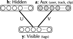
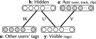
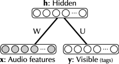
(a) (b) (c)

Figure 1: Schematic diagrams of the various restricted Boltzmann machines under investigation. (a) RBM for tag smoothing conditioned on just auxiliary information: user, track, clips identity, (b) RBM for tag smoothing conditioned on auxiliary information and tags of other users, (c) discriminative RBM for audio classification. Filled circles show variables that are always observed, open circles show variables that are inferred at test time.

RBMs can be conditioned on other variables [12]. In general, as shown in Figure 1(b), both the hidden and visible units can be conditioned on other variables, $\mathbf{u}=(v_{1},\ldots,v_{d})^{T}$ and $\mathbf{a}=(a_{1},\ldots,a_{A})^{T}$, respectively. Including these interactions, the energy function becomes

$$E(\mathbf{y},\mathbf{h},\mathbf{u},\mathbf{a})=-\mathbf{h}^{T}U\mathbf{y}-\mathbf{h}^{T}W\mathbf{u}-\mathbf{y}^{T}V\mathbf{a}-d^{T}\mathbf{y}-c^{T}\mathbf{h}$$ (6)

and $p(\mathbf{y},\mathbf{h}\,|\,\mathbf{u},\mathbf{a})\propto e^{-E(\mathbf{y},\mathbf{h},\mathbf{u},\mathbf{a})}$, where $W$ and $V$ are real matrices. The vectors $V\mathbf{a}$ and $W\mathbf{u}$ act like additional biases on $\mathbf{y}$ and $\mathbf{h}$. By setting the appropriate $W$ or $V$ matrix or conditioning vector $\mathbf{u}$ or $\mathbf{a}$ to 0, the conditioning can apply to only the visible units, as in Figure 1(a), or only the hidden units, as in Figure 1(c). For an observed data point $\mathbf{y}_{t},\mathbf{u}_{t},\mathbf{a}_{t}$, the gradient of the log likelihood with respect to a parameter $\theta$ becomes

$$\frac{\partial}{\partial\theta}\log p(\mathbf{y}_{t}\,|\,\mathbf{u}_{t},\mathbf{a}_{t})=-\mathbb{E}_{\mathbf{h}\,|\,\mathbf{y}_{t},\mathbf{u}_{t},\mathbf{a}_{t}}\left[\frac{\partial}{\partial\theta}E(\mathbf{y}_{t},\mathbf{h},\mathbf{u}_{t},\mathbf{a}_{t})\right]\\ +\mathbb{E}_{\mathbf{y},\mathbf{h}\,|\,\mathbf{u}_{t},\mathbf{a}_{t}}\left[\frac{\partial}{\partial\theta}E(\mathbf{y},\mathbf{h},\mathbf{u}_{t},\mathbf{a}_{t})\right].$$ (7)

[13] describes a conditional RBM used for collaborative filtering in which only the hidden variables are conditioned on other variables.

2.1 Conditional RBMs for tag smoothing

We first employ conditional RBMs to learn relationships among tags and between tags and users, tracks, and audio clips of tracks. This model is purely textual, meaning that it only operates on the tags and not on the audio.

All of the datasets used in this paper were collected by open endedly soliciting tags from users to describe audio clips. This means that the tags that they contain are most likely relevant, but the tags that are not present are not necessarily irrelevant. Thus there is a need to distinguish tags omitted but still relevant from those that do not apply, as well as tags that were included erroneously from those that truly apply. As shown in [14], the co-occurrences of tags can be used to predict both of these cases. For example, if the tags rap and hip-hop frequently co-occur and a clip has been tagged hip-hop but not rap, it would be reasonable to increase the likelihood of rap being relevant to that clip, although perhaps not as much as if it had actually been applied by a user. Similarly, it might be reasonable to decrease the likelihood of hip-hop being relevant as it was not corroborated by an application of rap.

We use the doubly conditional RBM shown in Figure 1(b) for this sort of tag “smoothing” as we call it. The binary visible units represent the tags that one user has applied to a clip and the hidden units capture second order relationships between these tags. The visible units are conditioned on auxiliary variables $\mathbf{a}$ which represent as one-hot vectors the user, track, and clip from which a vector of tags is observed. The hidden units are conditioned on auxiliary variables $\mathbf{u}$, which represent the tags that other users have applied to the same clip.

The vectors $\mathbf{y}$ and $\mathbf{u}$ are the same size, but whereas $\mathbf{y}$ is a binary vector representing which of the fixed vocabulary of tags the target user applied to the target clip, $\mathbf{u}$ is a vector of the average of these binary vectors for all of the other users who have seen the target clip. Thus the values in $\mathbf{u}$ are still between 0 and 1, but are continuous-valued. At test time, $\mathbf{u}$ is set to the average tag vector of all of the users and predicts the tags that a new user would likely apply to the clip given the tags that other users have already applied.

The weights $V$ and $W$ are penalized with an $\ell_{1}$ cost to encourage them to only capture dependencies that depend on specific settings of the auxiliary variables and push into $U$ the dependencies that exist independently of the auxiliary variables. This means that $V$ should ideally only capture tag information relevant to a particular user, clip, or track, $W$ should capture information about the relationships between other user’s tags and the current user’s tags, and $U$ should capture information about the co-occurrences of tags in general.

Compare this to the singly conditional RBM shown in Figure 1(a) and described in [14]. This CRBM also includes the conditioning of the visible units on the user, clip, and track information, but does not include the conditioning on other users’ tags. While the doubly conditional RBM can use its modeling power to learn to predict specific user’s tags from general tag patterns, this singly conditional model must predict both the general tag patterns and specific user’s tags, a harder problem. We found that the doubly-conditional RBM’s smoothing trains better SVMs on a validation experiment, and so we did not include the singly-conditional RBM in our experiments.

3 Discriminative RBMs

One useful variant of the conditional RBM is the discriminative RBM [9], shown in Figure 1(c). The discriminative RBM is a conditional RBM that is trained to predict the probability of the class labels, $\mathbf{y}$, from the rest of the inputs, $\mathbf{x}$. Based on the energy function of (6), it corresponds to setting $\mathbf{u}=\mathbf{x}$ and $\mathbf{a}=0$.

For a set of observed data points $\{(\mathbf{y}_{t},\mathbf{x}_{t})\}$, the discriminative RBM optimizes the log conditional, $\log p(\mathbf{y}_{t}\,|\,\mathbf{x}_{t})$, i.e. focusing on predicting $\mathbf{y}_{t}$ from $\mathbf{x}_{t}$ well. A generative variant of this RBM would instead optimize $\log p(\mathbf{y}_{t},\mathbf{x}_{t})$, the joint distribution (in this case, $\mathbf{x}_{t}$ acts as an extension of $\mathbf{y}_{t}$, i.e. it is not conditioned on it).

Looking at the parameter gradient of (7), we see that the second expectation requires a sum over all configurations of $\mathbf{y}$. When $\mathbf{y}$ can take only a few values, as in ordinary classification tasks [9], this expectation can be computed efficiently and exactly. However, here $\mathbf{y}$ is a set of $C$ binary indicators (the presence of a tag) that are not mutually exclusive, so that the expectation has $2^{C}$ terms and must be approximated because it cannot be computed in closed form. Note that given a value for $\mathbf{y}$, $p(\mathbf{h}|\mathbf{y},\mathbf{x}_{t})$ factors and is computed exactly.

3.1 Approximations to the expectation

In the case of the discriminative RBM involving $\mathbf{y}$, $\mathbf{h}$, $\mathbf{u}=\mathbf{x}$, and $\mathbf{a}=0$, we approximate the $\mathbb{E}_{\mathbf{y},\mathbf{h}\,|\,\mathbf{x}_{t}}$ term in (7) in three different ways: using contrastive divergence, mean-field contrastive divergence, and loopy belief propagation. We also compare a similar, but tractable computation that maximizes the pseudo-likelihood. The difficulty in computing this expectation stems directly from the difficulty in computing $p(\mathbf{y},\mathbf{h}\,|\,\mathbf{x}_{t})$, which in turn is caused by the interdependence of the $\mathbf{y}$ and $\mathbf{h}$ variables.

Contrastive divergence (CD) [11] has proven to be a very popular algorithm for estimating the log-likelihood gradient in RBMs, and it can also be used in the case of conditional RBMs. Typically, it is used to compute $\mathbb{E}_{\mathbf{y},\mathbf{x},\mathbf{h}}[\cdot]$ as opposed to here, where we compute $\mathbb{E}_{\mathbf{y},\mathbf{h}\,|\,\mathbf{x}_{t}}[\cdot]$. To compute the usual CD-$k$ update, $k$ steps of block Gibbs sampling, starting from the observed example $(\mathbf{x}_{t},\mathbf{y}_{t})$, are used to approximate the expectation. The block Gibbs chain is obtained by alternating sampling from $p(\mathbf{h}\,|\,\mathbf{y},\mathbf{x})$ and sampling from $p(\mathbf{y},\mathbf{x}\,|\,\mathbf{h})$. In the case of the conditional CD, we sample from $p(\mathbf{h}\,|\,\mathbf{y},\mathbf{x}_{t})$ and then from $p(\mathbf{y}\,|\,\mathbf{h})$ (since $\mathbf{h}$ isolates $\mathbf{y}$ from $\mathbf{x}_{t}$), keeping $\mathbf{x}_{t}$ fixed throughout. CD can be noisy because it uses a small number of samples (usually only one), and it can be biased because it doesn’t necessarily run the Markov chain to convergence (usually only 1 to 10 steps).

The mean-field contrastive divergence approach approximates the $\mathbf{y}$ and $\mathbf{h}$ variables using their conditional expectations (given each other) and iteratively updates each one based on the estimate of the other until convergence (note that $\mathbf{x}_{t}$ is fixed).

$$\mathbf{h}^{k} =\mathbb{E}[\mathbf{h}\,|\,\mathbf{y}^{k-1},\mathbf{x}_{t}]=\operatorname{sigm}(c+U\mathbf{y}^{k-1}+W\mathbf{x}_{t})$$ (8)

$$\mathbf{y}^{k} =\mathbb{E}[\mathbf{y}\,|\,\mathbf{h}^{k},\mathbf{x}_{t}]=\operatorname{sigm}(b+W\mathbf{h}^{k}).$$ (9)

In this case, we plug the continuous-valued expectations into these equations instead of the sampled binary values that should formally be used. While this method is straightforward, it cannot capture multimodal distributions in $\mathbf{y}$ and $\mathbf{h}$, which makes it sensitive to initialization. We set the initial condition $\mathbf{y}^{-1}=\mathbf{y}_{t}$, i.e. we initialize $\mathbf{y}$ at the training label from which we compute $\mathbf{h}^{0}$, etc., which is why this is referred to as mean-field contrastive divergence. We also tried to use standard mean-field where $\mathbf{y}^{-1}=0$, but found the results to be much worse.

Loopy belief propagation [15] (LBP) is another algorithm for approximating intractable marginals in a graphical model. It relies on a message passing procedure between the variables of the graph. While not guaranteed to converge it frequently does in practice, and gives estimates of the true marginals that are often more accurate than the iterative mean-field procedure [16]. In this setting, we used LBP to estimate the marginals $p(y_{j}=1|\mathbf{x}_{t})$, $p(h_{k}=1|\mathbf{x}_{t})$ and $p(y_{j}=1,h_{k}=1|\mathbf{x}_{t})$ for a given $\mathbf{x}_{t}$ under the discriminative RBM, and used those marginals to compute the $\mathbb{E}_{\mathbf{y},\mathbf{h}\,|\,\mathbf{x}_{t}}$ term in equation (7). The quantity $p(y_{j}=1|\mathbf{x}_{t})$ can also be estimated at test time to predict the labels. One method that has been shown to be useful in aiding convergence is message damped belief propagation [17]. In this case the updates computed by belief propagation are mixed with the previous updates for the same variables in order to smooth them, the damping factor being a parameter of the algorithm.

Another method for tuning the parameters aims to optimize not the likelihood of the data, but the pseudo-likelihood [18]. The pseudo-likelihood circumvents the intractability of computing the partition function in (3) by considering only configurations of the visible units that are within a Hamming distance of 1 from the training observation.

$$\log PL(\mathbf{y}\,|\,\mathbf{x}) =\sum_{j}\log p(y_{j}\,|\,\mathbf{y}_{\backslash j},\mathbf{x})$$ (10)

$$=\sum_{j} \log p(\mathbf{y}\,|\,\mathbf{x})-\log\left(p(\mathbf{y}\,|\,\mathbf{x})+p(\tilde{\mathbf{y}}_{j}\,|\,\mathbf{x})\right)$$

where $\mathbf{y}_{\backslash j}$ is the labels vector $\mathbf{y}$ without the $j$th variable and $\tilde{\mathbf{y}}_{j}$ is the labels vector $\mathbf{y}$ with the $j$th bit flipped (the subscript $t$ is removed here for clarity). The pseudo-likelihood can be optimized using gradient descent.

Because of lack of space, we give pseudocodes for all the aforementioned algorithms in the appendix. Additionally, the python code used for training these models is available on our website. Note that while all of these methods can be used for training, not all of them can be used at test time to estimate $P(y_{j}=1|\mathbf{x}_{t})$. Specifically, the pseudo-likelihood requires the knowledge of $\mathbf{y}_{\backslash i}$, which is unavailable at test time. Similarly, CD must be initialized from the true values of $\mathbf{y}_{t}$ and $\mathbf{x}_{t}$. It is possible to use a Gibbs sampling method similar to CD starting from an arbitrary initialization of $\mathbf{y}_{t}$, but this is costly because the Markov chain may need to be run for many iterations before it mixes well. We found that mean-field CD could be successfully initialized with $\mathbf{y}^{-1}=0$ at test time.

4 Experiments

We performed a number of experiments to compare different hyper-parameter settings, to compare different classifiers, and to compare different tag smoothing techniques. These experiments were based on three different datasets: data from Amazon.com’s Mechanical Turk service, data from the MajorMiner music labeling game, and data from Last.fm’s users. We compare the discriminative RBM to standard (generative) RBMs, multi-layer perceptrons, logistic regression, and support vector machines. All of these algorithms were evaluated in terms of retrieval performance using the area under the ROC curve.

4.1 Datasets

Three datasets were used in these experiments. All of these datasets were in the form of (user, item, tag) triples, where the items were either 10-second clips of tracks or whole tracks. These data were condensed into (item, tag, count) triples by summing across users.

The first dataset was collected from Amazon.com’s Mechanical Turk service and is described in [14]. Users were asked to describe 10-second clips of songs in terms of 5 broad categories including genre, emotion, instruments, and overall production. The music used in the experiment consisted of 185 songs selected randomly from the music blogs indexed by the Hype Machine. From each track, five 10-second clips were extracted from proportionally equally spaced points, for a total of 925 clips. Each clip was seen by a total of 3 users, generating approximately 15,500 (user, clip, tag) triples from 210 unique users. We used the most popular 77 tags for this dataset.

The second dataset was collected from the MajorMiner music labeling game and is described in [7]. Players were asked to describe 10-second clips of songs and were rewarded for agreeing with other players and for being original. This dataset includes approximately 80,000 (user, clip, tag) triples with 2600 unique clips, 650 unique users, and 1000 unique tags. We used the most popular 77 tags for this dataset.

The final dataset was collected from Last.fm’s website and is described in [19]. The entire dataset consists of approximately 7 million (user, track, tag) triples from 84,000 unique users, 1 million unique tracks, and 280,000 unique tags. While only the textual information was collected from Last.fm, we were able to match it to 47,000 tracks in our own music collection. While this may seem like a small fraction of the total number of tracks, the tracks that were found included 1.5 million of the (user, track, tag) triples, implying that the tracks we were able to match were tagged more often than average. Following similar reasoning, many of these users, tracks, and tags occurred infrequently, with 1 million (user, track, tag) triples in which all three items occurred in at least 25 triples. Because these tags were applied at the track level and not at the clip level, we selected one clip from the center of each track and assumed that they should all be described with the track tags. This is the simplest solution to this problem, although using some form of multiple-instance learning might find a better solution [20]. We used the most popular 100 tags for this dataset.

Converting (item, tag, count) triples to binary matrices for training and evaluation purposes required some care. In the MajorMiner and Last.fm data, the counts were high enough that we could require the verification of an (item, tag) pair by at least two people, meaning that the count had to be at least 2 to be considered as a positive example. The Mechanical Turk dataset did not have high enough counts to allow this, so we had to count every (item, tag) pair. In the MajorMiner and Last.fm datasets, (item, tag) pairs with only a single count were not used as negative examples because we assumed that they had higher potential relevance than (item, tag) pairs that never occurred, which served as stronger negative examples.

Features

The timbral and rhythmic features of [7] were used to characterize the audio of 10-second song clips. The timbral features were the mean and rasterized full covariance of the clip’s mel frequency cepstral coefficients. They capture information about instrumentation and overall production qualities. The rhythmic features are based on the modulation spectra in four large frequency bands. In fact, they are closely related to the autocorrelation in those frequency bands. They capture information about the rhythm of the various parts of the drum kit (if present), i.e. bass drum, tom tom, snare, hi-hat. They also discriminate between music that has a strong rhythmic component, e.g. dance music, and music that does not, e.g. folk rock. Each dimension of both sets of features was normalized across the database to have zero-mean and unit-variance, and then each feature vector was normalized to be unit norm to reduce the effect of outliers. The timbral features were 189-dimensional and the rhythmic features were 200-dimensional, making the combined feature vector 389-dimensional.

4.2 Classifiers

We compared a number of classifiers including two variants of restricted Boltzmann machines, and three other standard classifiers. The RBMs we compared were the discriminative RBM, described in Section 3 and a standard generative RBM. Both RBMs use Gaussian input units [21] in order to deal with the continuous-valued features for $\mathbf{x}$. The other classifiers include a multi-layer perceptron, logistic regression, and support vector machines. For all datasets we select the hyper-parameters of the model using a 5-fold cross-validation. In order to increase accuracy of our measure, for each fold we computed the score as an average across 4 sub-folds. Each run used a different fold (from the remaining 4 folds) as the validation set and the other 3 as the training set.

The discriminative RBM uses the gradient updates shown in (7), while the generative RBM uses a different update in which the second expectation is $\mathbb{E}_{\mathbf{y},\mathbf{x},\mathbf{h}}$ instead of $\mathbb{E}_{\mathbf{y},\mathbf{h}\,|\,\mathbf{x}_{t}}$. The generative RBM attempts to maximize $\log p(\mathbf{y},\mathbf{x})$, while the discriminative RBM attempts to maximize $\log p(\mathbf{y}\,|\,\mathbf{x})$. It is also possible to use a mixture of these two objective functions and maximize $\alpha\log p(\mathbf{y},\mathbf{x})+\log p(\mathbf{y}\,|\,\mathbf{x})$, referred to as a hybrid generative/discriminative RBM [9]. In our experiments, however, the hybrid RBM did not improve on the DRBM, so we will not discuss it further. For each model and dataset pair we optimized the hyper-parameters using the cross validation described above, selecting the hyper-parameters with the best performance on the validation set averaging across folds and tags. Different hyper-parameters performed best in each case, which is to be expected given the differences in the models and in the data. For example, one would expect the generative RBM to require more hidden units than the discriminative RBM because it models the joint probability. Also on a large dataset, one would expect to be able to use more hidden units without overfitting. The hyper-parameters that performed best on the validation set can be seen in Table 1.

Table 1: Parameter settings found to perform best on validation sets and used in experiments for discriminative and generative RBMs, multi-layer perceptrons, and logistic regression. LR stands for learning rate.

		Number of hidden units
Model	LR	MTurk	MajMin	Last.fm
Disc. RBM	0.01	50	100	200
Gen. RBM	0.01	200	300	300
MLP	0.001	250	250	250
Log. reg.	2.0	—	—	—

The multi-layer perceptron (MLP) is quite similar in structure to the discriminative RBM in that it has nodes representing the features and the classes and hidden nodes that capture interactions between them. The main difference is that in estimating $p(\mathbf{y}\,|\,\mathbf{x})$ there is no modeling of the interactions between the elements of $\mathbf{y}$ given $\mathbf{x}$. In the discriminative RBM, at test time the unknown $\mathbf{y}$ and $\mathbf{h}$ interact with one another through one of the methods described in Section 3.1 until they reach a mutually agreeable equilibrium. In the case of the MLP, however, at test time $\mathbf{h}$ is computed deterministically from $\mathbf{x}$ and $\mathbf{y}$ is computed deterministically from $\mathbf{h}$. The stochastic hidden units in the discriminative RBM at test time allow it to better capture interactions between the variables in $\mathbf{y}$ (i.e. the tags).

An even simpler classifier than the MLP is logistic regression, which has no hidden layer and predicts each class directly from the input features. We similarly optimize this using gradient descent, where the cost function is the cross-entropy between the target labels and the predictions, like for the MLP.

The final classifier we compared is the support vector machine (SVM). Specifically we used a linear kernel and a $\nu$-SVM [22] to automatically select the $C$ parameter. We trained a different SVM for each tag as an independent two-way decision (e.g. rock vs not rock). While the above methods based on stochastic gradient descent can be trained on all examples, SVMs are more sensitive to the relative number of positive and negative examples, so we had to more carefully select the training examples to use for each tag. To do this, we selected as positive examples those clips to which users applied a given tag most frequently and as negative examples those clips to which users applied a given tag least frequently (generally 0 times). The actual training labels used, however, were still the standard $\pm 1$ targets. We ensured that there were the same number of positive and negative examples, up to 200 of each.

Metrics

The performance of all of these algorithms on all of these datasets is evaluated in terms of retrieval performance using the area under the ROC curve (AUC) [23]. This metric scores the ability of an algorithm to rank relevant examples in a collection above irrelevant examples. A random ranking will achieve an AUC of approximately 0.5, while a perfect ranking will achieve an AUC of 1.0. In certain experiments CRBMs were used to smooth the training data, but the testing data was always the unsmoothed, user-supplied tags. We measure the AUC for each tag separately. We use the average across tags and folds as a overall measure of performance and consider the standard error across folds for Figure 3. For a more detailed comparison we use a two-sided paired t-test across folds, per tag, between two models. We count the number of tags for which each model performs better than the other at a 95% significance level.

Implementation details / Running time

In order to find the parameters that worked best for the DRBM, we used a grid search. To avoid a prohibitive number of combinations, we settled on a learning rate and number of hidden units before exploring gradient approximations, Loopy Belief Propagation damping factors, and numbers of iterations for CD, MF-CD or LBP. We also performed a much wider parameter search on the smaller datasets, MTurk and MajorMiner, keeping the same parameters for Last.fm, but varying the number of hidden units. We found that the DRBM is insensitive to the number of iteration steps while the computational cost increases considerably. Training time varies according to many details, but on average, to train a DRBM on MajorMiner took around 48 CPU-hours.

4.3 Experiments

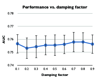
Figure 2: Average area under the ROC curve with standard errors on the MajorMiner dataset for the discriminative RBM trained using loopy belief propagation with different damping factors.

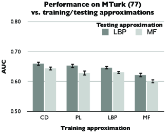
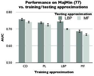
Figure 3: Results on Mechanical Turk and MajorMiner comparing the performance of different approximations for the discriminative RBM during training and testing: contrastive divergence (CD), pseudo-likelihood (PL), mean field contrastive divergence (MF) and loopy belief propagation (LBP). The approximations used during training are represented on the x-axis, while the approximations used during testing are represented through the gray value of the bar.

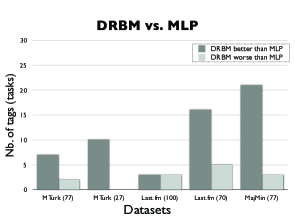
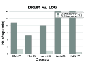
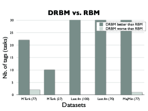
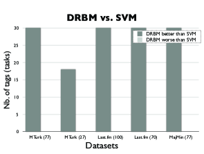
Figure 4: Comparison of discriminative restricted Boltzmann machine autotagging retrieval performance to multi-layered perceptron (MLP), logistic regression (LOG), (generative) restricted Boltzmann machine (RBM), and support vector machine (SVM). Each bar shows performance on a different dataset and its height is the number of tags on which a two-sided paired t-test showed one algorithm to be significantly better than the other in terms of area under the ROC curve. Tags that were not significantly different are not included in this plot.

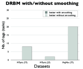
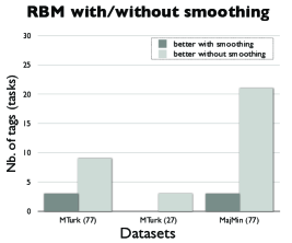
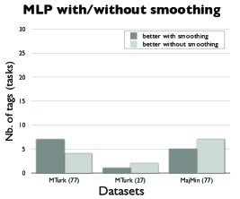
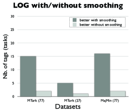
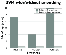
Figure 5: Comparison of autotagging retrieval performance with and without conditional restricted Boltzmann machine-based smoothing for discriminative restricted Boltzmann machine (DRBM), multi-layer perceptron (MLP), (generative) restricted Boltzmann machine (RBM), logistic regression (LOG) and support vector machine (SVM). Bars show number of tags on which one set of autotaggers was significantly better, as in Figure 4.

Table 2: Average AROC across tags as a percentage for each algorithm on each dataset with a specified number of tags (Tgs) and with and without tag smoothing (Sm).

Dataset	Tgs	Sm	DRBM	MLP	RBM	LOG	SVM
MTurk	27	$-$	68.8	65.4	65.4	65.7	62.3
MTurk	27	$+$	68.4	65.6	64.6	66.7	66.0
MTurk	77	$-$	65.9	65.8	62.9	63.4	59.2
MTurk	77	$+$	65.9	66.1	62.4	64.6	64.0
MajMin	77	$-$	76.1	75.3	70.0	70.7	64.5
MajMin	77	$+$	74.8	74.8	68.2	73.3	71.5
Last.fm	70	$-$	72.2	72.0	65.9	70.3	64.6
Last.fm	100	$-$	72.4	72.4	66.1	70.2	64.5

Experiment 1

The first experiment measured the effectiveness of different settings of the smoothing hyper-parameter in loopy belief propagation, meant to aid the convergence of the algorithm. Figure 2 shows the mean area under the ROC curve (AUC) on the MajorMiner dataset of discriminative RBMs trained using loopy belief propagation (LBP) with different damping factors. We use 10 training iterations. The plots show that the damping factor does not change the accuracy of the model appreciably. Very similar results were obtained on the MTurk dataset (not shown), while for Last.fm dataset we only use $\beta=0.9$ which performed best on MTurk.

Experiment 2

The second experiment compared discriminative RBMs trained and tested with different combinations of approximations to the intractable expectation in (7). We use different approximations on train and test to fully explore the space of possibilities. The left plot in Figure 3 shows the mean AUC of these discriminative RBMs on the MTurk dataset, while the right plot shows the same results for MajorMiner. The four training approximations, in order of performance on MTurk, were contrastive divergence (CD), pseudo-likelihood (PL), loopy belief propagation (LBP) and mean-field contrastive divergence (MF). On MajorMiner the same order was preserved, except that loopy belief propagation outperformed pseudo-likelihood. The testing approximations, in order of performance were LBP and mean-field (MF). The training approximation had a larger impact on the final result than the testing approximation. For Last.fm we only used CD during training and LBP at test time. We also found that the model is quite robust to the number of training or testing iterations for CD, MF or LBP.

Experiment 3

The third experiment compares the different classifiers on the three datasets with and without tag smoothing. We have also added a slight variation of the MTurk and Last.fm datasets restricted to a subset of the most popular tags (27 for MTurk and 70 for Last.fm). Using a two-sided paired t-test per tag, we compare all models to a discriminative restricted Boltzmann machine trained on unsmoothed data. The same test is done against all of the comparison models: multi-layer perceptron (MLP), logistic regression (LOG), generative RBM (RBM), and support vector machines (SVM). Figure 4 shows the number of tags on which the DRBM outperforms the other algorithm. The DRBM outperforms all of the other algorithms on many more tags than it is outperformed. The MLP is evenly matched to it on the full Last.fm 100 dataset, but on the other four datasets, the DRBM is significantly better on many more tags than it is worse. The SVM and logistic regression were previously the best performing algorithms on these datasets.

Figure 5 shows the same analysis comparing each classifier trained on the raw, user-supplied tags to the same classifier trained on the tags smoothed by the proposed tag smoothing conditional RBM. Different subsets of the auxiliary inputs were compared and the smoothing that gave the best performance on the validation folds was selected. Because of the size of the Last.fm dataset, only the unsmoothed tags were tested. A number of interesting trends are visible in Figure 5. First, the SVM and logistic regression models are helped by the tag smoothing. This makes sense because they treat each tag as a separate classification task and cannot by themselves take advantage of the relationships between tags. The MLP was sometimes helped by tag smoothing, but generally was not. The fact that the RBMs were not helped by the tag smoothing suggests that they are able to capture by themselves the relationships between tags and do not need the assistance of the tag smoothing.

5 Conclusion

This paper has described two applications of conditional restricted Boltzmann machines to the task of autotagging music. The discriminative RBM was able to achieve a higher average area under the ROC curve than the previously best known system for this problem, the support vector machine, as well as the multi-layer perceptron and logistic regression. In order to be applied to this problem, the discriminative RBM was generalized to the multi-label setting and an in-depth analysis of four different learning algorithms for it were evaluated. The best results were obtained for a DRBM using contrastive divergence training and loopy belief propagation at test time. The performance of the SVM was improved significantly, although not to the level of the DRBM, by the purely textual tag smoothing conditional RBM. Both of these results demonstrate the power of modeling the relationships between tags in autotagging systems.

Appendix A Appendix: Pseudocode

A discriminative RBM is based on the following energy function:

$$E(\mathbf{y},\mathbf{h},\mathbf{x})=-\mathbf{h}^{T}U\mathbf{y}-\mathbf{h}^{T}W\mathbf{x}-b^{T}\mathbf{y}-c^{T}\mathbf{h}$$ (11)

where $\mathbf{x}$ is conditioned on. From this energy function, we can define a probability distribution over $\mathbf{y}$ and $\mathbf{h}$ as follows: $p(\mathbf{y},\mathbf{h}\,|\,\mathbf{x})\propto e^{-E(\mathbf{y},\mathbf{h},\mathbf{x})}$.

In the next sections, we describe the different approaches we evaluated for training such an RBM.

A.1 Contrastive Divergence

The most straighforward approach is perhaps to train the RBM to maximise the conditional log-likelihood of the associated target vector $\mathbf{y}$ by gradient descent. To do so, we need to estimate the following gradient:

$$\frac{\partial}{\partial\theta}\log p(\mathbf{y}_{t}\,|\,\mathbf{x}_{t})=-\mathbb{E}_{\mathbf{h}\,|\,\mathbf{y}_{t},\mathbf{x}_{t}}\left[\frac{\partial}{\partial\theta}E(\mathbf{y}_{t},\mathbf{h},\mathbf{x}_{t})\right]\\ +\mathbb{E}_{\mathbf{y},\mathbf{h}\,|\,\mathbf{x}_{t}}\left[\frac{\partial}{\partial\theta}E(\mathbf{y},\mathbf{h},\mathbf{x}_{t})\right].$$ (12)

Since the second $\mathbb{E}_{\mathbf{y},\mathbf{h}\,|\,\mathbf{x}_{t}}$ is intractable, we need to approximate it somehow. The contrastive divergence algorithm [11] proposes to replace this expectation by a point estimate at a sample $\mathbf{y}^{K}$, obtained by running a Gibbs sampling initialized at $\mathbf{y}$ for $K$ iterations. Given a sample $\mathbf{y}^{K}$ and given $\mathbf{x}_{t}$, the expectation with respect to $\mathbf{h}$ is now tractable.

Algorithm 1 describes the associated training update, given an example $(\mathbf{y},\mathbf{x})$. In our notation, $a\leftarrow b$ means $a$ is set to value $b$ and $a\sim p$ means $a$ is sampled from the distribution $p$.

Algorithm 1 Discriminative RBM training update using Contrastive Divergence.

  Input: training pair $(\mathbf{y},\mathbf{x})$, number of iterations $K$ and learning rate $\lambda$

  # Positive phase

  $\mathbf{y}^{0}\leftarrow\mathbf{y}$, $\widehat{\mathbf{h}}^{0}\leftarrow\operatorname{sigm}(c+W\mathbf{x}+U\mathbf{y}^{0})$

  

  # Negative phase ( we are doing CD-K here)

  for $K$ iterations do

     $\mathbf{h}^{k}\sim p(\mathbf{h}|\mathbf{y}^{k},\mathbf{x})$

     $\mathbf{y}^{k+1}\sim p(\mathbf{y}|\mathbf{h}^{k})$

     $\widehat{\mathbf{h}}^{k+1}\leftarrow\operatorname{sigm}(c+W\mathbf{x}+U\mathbf{y}^{k+1})$

  end for

  

  # Update

  for $\theta\in\Theta$ do

     $\theta\leftarrow\theta-\lambda\left(\frac{\partial}{\partial\theta}E(\mathbf{y}^{0},\mathbf{x},\widehat{\mathbf{h}}^{0})-\frac{\partial}{\partial\theta}E(\mathbf{y}^{K},\mathbf{x},\widehat{\mathbf{h}}^{K})\right)$

  end for

A.2 Mean-Field Contrastive Divergence

A non-stochastic alternative to contrastive divergence is mean-field contrastive divergence [24], where samples are replaced by expectations. This procedure is detailed in Algoritm 2.

Algorithm 2 Discriminative RBM training update using Mean-Field Contrastive Divergence.

  Input: training pair $(\mathbf{y},\mathbf{x})$, number of iterations $K$ and learning rate $\lambda$

  # Positive phase

  $\widehat{\mathbf{y}}^{0}\leftarrow\mathbf{y}$, $\widehat{\mathbf{h}}^{0}\leftarrow\operatorname{sigm}(c+W\mathbf{x}+U\widehat{\mathbf{y}}^{0})$

  

  # Negative phase ( we are doing MFCD-K here)

  for $K$ iterations do

     $\widehat{\mathbf{y}}^{k+1}\leftarrow\operatorname{sigm}(d+U^{T}\widehat{\mathbf{h}}^{k})$

     $\widehat{\mathbf{h}}^{k+1}\leftarrow\operatorname{sigm}(c+W\mathbf{x}+U\widehat{\mathbf{y}}^{k+1})$

  end for

  

  # Update

  for $\theta\in\Theta$ do

     $\theta\leftarrow\theta-\lambda\left(\frac{\partial}{\partial\theta}E(\widehat{y}^{0},\mathbf{x},\widehat{\mathbf{h}}^{0})-\frac{\partial}{\partial\theta}E(\widehat{y}^{K},\mathbf{x},\widehat{\mathbf{h}}^{K})\right)$

  end for

A.3 Loopy Belief Propagation

Instead of using a sample $\mathbf{y}^{K}$ to approximate the intractable expectation, one could try to estimate directly the associated marginals required by this expectation. Specifically, those marginals are $p(y_{j}=1|\mathbf{x})$, $p(h_{k}=1|\mathbf{x})$ and $p(y_{j}=1,h_{k}=1|\mathbf{x})$. Loopy belief propagation [15] is a popular algorithm for approximating such marginals. Algorithm 3 details this procedure for the discriminative RBM. The given algorithm computes messages in log-space and, for computational efficiency, messages are normalized so that log-messages from zero-valued variables is 0 (hence only messages from one-valued variables are passed).

Algorithm 3 Loopy Belief Propagation algorithm for inference in discriminative RBM

  Input: training pair $(\mathbf{y},\mathbf{x})$, number of iterations $K$ and damping factor $\beta$

  $m_{kj}^{\uparrow}\leftarrow 0,~{}~{}m_{kj}^{\downarrow}\leftarrow 0$    $\forall~{}j,k$

  $c^{\rm data}\leftarrow c+W\mathbf{x}$

  

  # Update downwards (towards $\mathbf{y}$) and upwards (towards $\mathbf{h}$) messages

  for $K$ iterations do

     $m_{kj}^{\downarrow}\leftarrow\beta m_{kj}^{\downarrow}+(1-\beta)\log\left(1+(\exp(U_{kj})-1)~{}\operatorname{sigm}(c^{\rm data}_{k}+\sum_{j^{*}\neq j}m_{kj^{*}}^{\uparrow})\right),$    $\forall~{}j,k$

     $m_{kj}^{\uparrow}\leftarrow\beta m_{kj}^{\uparrow}+(1-\beta)\log\left(1+(\exp(U_{kj})-1)~{}\operatorname{sigm}(d_{j}+\sum_{k^{*}\neq k}m_{k^{*}j}^{\downarrow})\right),$    $\forall~{}j,k$

  end for

  

  # Compute estimated singleton and pair-wise marginals

  $p^{\rm LBP}(y_{j}=1|\mathbf{x})\leftarrow\operatorname{sigm}(d_{j}+\sum_{k}m_{kj}^{\downarrow}),$    $\forall~{}j$

  $p^{\rm LBP}(h_{k}=1|\mathbf{x})\leftarrow\operatorname{sigm}(c^{\rm data}_{k}+\sum_{j}m_{kj}^{\uparrow}),$    $\forall~{}k$

  

  ${\rm num}^{01}_{kj}\leftarrow d_{j}+\sum_{k^{*}\neq k}m_{k^{*}j}^{\downarrow},~{}~{}{\rm num}^{10}_{kj}\leftarrow c^{\rm data}_{k}+\sum_{j^{*}\neq j}m_{kj^{*}}^{\uparrow},$    $\forall~{}j,k$

  ${\rm num}^{11}_{kj}\leftarrow U_{kj}+{\rm num}^{10}_{kj}+{\rm num}^{01}_{kj},$    $\forall~{}j,k$

  $p^{\rm LBP}(y_{j}=1,h_{k}=1|\mathbf{x})=\exp({\rm num}^{11}_{kj})/(\exp({\rm num}^{11}_{kj})+\exp({\rm num}^{01}_{kj})+\exp({\rm num}^{10}_{kj})),$    $\forall~{}j,k$

A.4 Pseudo-likelihood training

Finally, instead of approximately estimating the gradient of the log-likelihood $\log p(\mathbf{y}_{t}\,|\,\mathbf{x}_{t})$, one could instead replace it by the pseudo-likelihood objective [18]:

$$\log PL(\mathbf{y}\,|\,\mathbf{x}) =\sum_{j}\log p(y_{j}\,|\,\mathbf{y}_{\backslash j},\mathbf{x})$$ (13)

$$=\sum_{j} \log p(\mathbf{y}\,|\,\mathbf{x})-\log\left(p(\mathbf{y}\,|\,\mathbf{x})+p(\tilde{\mathbf{y}}_{j}\,|\,\mathbf{x})\right)$$

and compute its gradient exactly. Algorithm 4 details the procedure for updating the RBM according to that criteria.

Algorithm 4 Pseudo-likelihood training update algorithm in discriminative RBM

  Input: training pair $(\mathbf{y},\mathbf{x})$, learning rate $\lambda$

  

  # Forward propagation

  $c^{\rm data}\leftarrow c+W\mathbf{x}+U\mathbf{y}$

  $\log PL(\mathbf{y}\,|\,\mathbf{x})\leftarrow 0$

  for $j$ from 1 to $|\mathbf{y}|$ do

     $p(y_{j}\,|\,\mathbf{y}_{\backslash j},\mathbf{x})\leftarrow\operatorname{sigm}\left\{d_{j}+\sum_{k}\log\left[1+\exp(c^{\rm data}_{k}-U_{kj}y_{j}+U_{kj})\right]-\log\left[1+\exp(c^{\rm data}_{k}-U_{kj}y_{j})\right]\right\}$

     $\log PL(\mathbf{y}\,|\,\mathbf{x})\leftarrow\log PL(\mathbf{y}\,|\,\mathbf{x})-y_{j}\log p(y_{j}\,|\,\mathbf{y}_{\backslash j},\mathbf{x})-(1-y_{j})\log(1-p(y_{j}\,|\,\mathbf{y}_{\backslash j},\mathbf{x}))$

  end for

  

  # Backward propagation

  $\partial U\leftarrow 0$, $\partial W\leftarrow 0$, $\partial c\leftarrow 0$

  for $j$ from 1 to $|\mathbf{y}|$ do

     $\partial{\rm out}_{j}\leftarrow p(y_{j}\,|\,\mathbf{y}_{\backslash j},\mathbf{x})-y_{j},$ $\partial d_{j}\leftarrow\partial{\rm out}_{j},$ $\partial{\rm hid}\leftarrow 0$

     for $k$ from 1 to $|\mathbf{h}|$ do

        $\partial U_{kj}\leftarrow\partial U_{kj}+\partial{\rm out}_{j}~{}((1-y_{j})~{}\operatorname{sigm}(c^{\rm data}_{k}-U_{kj}y_{j}+U_{kj})+y_{j}~{}\operatorname{sigm}(c^{\rm data}_{k}-U_{kj}y_{j}))$

        $\partial{\rm hid}_{k}\leftarrow\partial{\rm out}_{j}~{}(\operatorname{sigm}(c^{\rm data}_{k}-U_{kj}y_{j}+U_{kj})-\operatorname{sigm}(c^{\rm data}_{k}-U_{kj}y_{j}))$

     end for

     $\partial U\leftarrow\partial U+\partial{\rm hid}~{}\mathbf{y}^{T},$ $\partial W\leftarrow\partial W+\partial{\rm hid}~{}\mathbf{x}^{T},$ $\partial c\leftarrow\partial c+\partial{\rm hid}$

  end for

  

  # Update

  $U\leftarrow U-\lambda~{}\partial U,$ $W\leftarrow W-\lambda~{}\partial W,$ $c\leftarrow c-\lambda~{}\partial c,$ $d\leftarrow d-\lambda~{}\partial d$

References

- [1] P. Lamere. Social tagging and music information retrieval. J. New Music Res., 37(2):101–114, 2008.
- [2] A. I. Schein, A. Popescul, L. H. Ungar, and D. M. Pennock. Methods and metrics for cold-start recommendations. In Proc. Intl. ACM SIGIR Conf. on Research and development in information retrieval, pages 253–260, 2002.
- [3] B. Whitman and R. Rifkin. Musical query-by-description as a multiclass learning problem. In IEEE Workshop on Multimedia Signal Processing, pages 153–156, 2002.
- [4] D. Eck, P. Lamere, T. Bertin-Mahieux, and S. Green. Automatic generation of social tags for music recommendation. In J.C. Platt, D. Koller, Y. Singer, and S. Roweis, editors, NIPS 20. MIT Press, 2008.
- [5] D. Tingle, Y. E. Kim, and D. Turnbull. Exploring automatic music annotation with ”acoustically-objective” tags. In Proc. Intl. Conf. on Multimedia information retrieval, pages 55–62. ACM, 2010.
- [6] T. Bertin-Mahieux, D. Eck, F. Maillet, and P. Lamere. Autotagger: A model for predicting social tags from acoustic features on large music databases. J. New Music Res., 37(2):115––135, 2008.
- [7] M. I. Mandel and D. P. W. Ellis. A web-based game for collecting music metadata. J. New Music Res., 37(2):151–165, 2008.
- [8] K. Trohidis, G. Tsoumakas, G. Kalliris, and I. Vlahavas. Multilabel classification of music into emotions. In Proc. ISMIR, 2008.
- [9] H. Larochelle and Y. Bengio. Classification using discriminative restricted Boltzmann machines. In Andrew McCallum and Sam Roweis, editors, Proc. ICML, pages 536–543. Omnipress, 2008.
- [10] P. Smolensky. Information processing in dynamical systems: foundations of harmony theory. MIT Press, 1986.
- [11] G. Hinton. Training products of experts by minimizing contrastive divergence. Neural Computation, 14:1771–1800, 2002.
- [12] G. Taylor, G. E. Hinton, and S. Roweis. Modeling human motion using binary latent variables. In B. Schölkopf, J. Platt, and T. Hoffman, editors, NIPS 19, pages 1345–1352. MIT Press, Cambridge, MA, 2007.
- [13] R. Salakhutdinov, A. Mnih, and G. Hinton. Restricted Boltzmann machines for collaborative filtering. In Proc. ICML, pages 791–798, 2007.
- [14] M. I. Mandel, D. Eck, and Y. Bengio. Learning tags that vary within a song. In Proceedings of the 11th International Conference on Music Information Retrieval (ISMIR), pages 399–404, August 2010.
- [15] K. P. Murphy, Y. Weiss, and M. I. Jordan. Loopy belief propagation for approximate inference: An empirical study. In Proc. Uncertainty in AI, pages 467–475, 1999.
- [16] Y. Weiss. Comparing the mean field method and belief propagation for approximate inference in MRFs. In Advanced Mean Field Methods - Theory and Practice. MIT Press, 2001.
- [17] M. Pretti. A message-passing algorithm with damping. Journal of Statistical Mechanics: Theory and Experiment, page P11008, 2005.
- [18] J. Besag. Statistical analysis of non-lattice data. The Statistician, 24(3):179–195, 1975.
- [19] R. Schifanella, A. Barrat, C. Cattuto, B. Markines, and F. Menczer. Folks in folksonomies: Social link prediction from shared metadata. In Proc. ACM Intl. Conf. on Web search and data mining, pages 271–280. ACM, Mar 2010.
- [20] M. I. Mandel and D. P. W. Ellis. Multiple-instance learning for music information retrieval. In Proc. ISMIR, pages 577–582, September 2008.
- [21] M. Welling, M. Rosen-Zvi, and G. E. Hinton. Exponential family harmoniums with an application to information retrieval. In L.K. Saul, Y. Weiss, and L. Bottou, editors, NIPS 17, volume 17, Cambridge, MA, 2005. MIT Press.
- [22] B. Schölkopf, A. J. Smola, R. C. Williamson, and P. L. Bartlett. New support vector algorithms. Neural Comput., 12(5):1207–1245, May 2000.
- [23] C. Cortes and M. Mohri. Auc optimization vs. error rate minimization. In S. Thrun, L. Saul, and B. Schölkopf, editors, NIPS 16, volume 16, Cambridge, MA, 2004. MIT Press.
- [24] Max Welling and Geoffrey E. Hinton. A new learning algorithm for mean field Boltzmann machines. In ICANN ’02: Proceedings of the International Conference on Artificial Neural Networks, pages 351–357, London, UK, 2002. Springer-Verlag.