Cyber-Physical Attacks in Power Networks:
Models, Fundamental Limitations and Monitor Design

Abstract

Future power networks will be characterized by safe and reliable functionality against physical malfunctions and cyber attacks. This paper proposes a unified framework and advanced monitoring procedures to detect and identify network components malfunction or measurements corruption caused by an omniscient adversary. We model a power system under cyber-physical attack as a linear time-invariant descriptor system with unknown inputs. Our attack model generalizes the prototypical stealth, (dynamic) false-data injection and replay attacks. We characterize the fundamental limitations of both static and dynamic procedures for attack detection and identification. Additionally, we design provably-correct (dynamic) detection and identification procedures based on tools from geometric control theory. Finally, we illustrate the effectiveness of our method through a comparison with existing (static) detection algorithms, and through a numerical study.

I Introduction

Problem setup Recent studies and real-world incidents have demonstrated the inability of the power grid to ensure a reliable service in the presence of network failures and possibly malignant actions [1, 2]. Besides failures and attacks on the physical power grid infrastructure, the envisioned future smart grid is also prone to cyber attacks on its communication layer. In short, cyber-physical security is a fundamental obstacles challenging the smart grid vision.

A classical mathematical model to describe the grid on the transmission level is the so-called structure-preserving power network model, which consists of the dynamic swing equation for the generator rotor dynamics, and of the algebraic load-flow equation for the power flows through the network buses [3]. In this work, we consider the linearized small signal version of the structure-preserving model, which is composed by the linearized swing equation and the DC power flow equation. The resulting linear continuous-time descriptor model of a power network has also been studied for estimation and security purposes in [4, 5, 6].

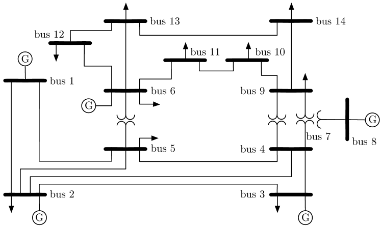
Figure 1: For the here represented IEEE 14 bus system, if the voltage angle of one bus is measured exactly, then a cyber attack against the measurements data is always detectable by our dynamic detection procedure. In contrary, as shown in [7], a cyber attack may remain undetected by a static procedure if it compromises as few as four measurements.

From static to dynamic detection Existing approaches to security and stability assessment are mainly based upon static estimation techniques for the set of voltage angles and magnitudes at all system buses, e.g., see [8]. Limitations of these techniques have been often underlined, especially when the network malfunction is intentionally caused by an omniscient attacker [7, 9]. The development of security procedures that exploit the dynamics of the power network is recognized [10] as an outstanding important problem. We remark that the use of static state estimation and detection algorithms has been adopted for many years for several practical and technological reasons. First, because of the low bandwidth of communication channels from the measuring units to the network control centers, continuous measurements were not available at the control centers, so that the transient behavior of the network could not be captured. Second, a sufficiently accurate dynamic model of the network was difficult to obtain or tune, making the analysis of the dynamics even harder. As of today, because of recent advances in hardware technologies, e.g., the advent of Phasor Measurement Units and of large bandwidth communications, and in identification techniques for power system parameters [11], these two limitations can be overcome. Finally, a dynamic estimation and detection problem was considered much harder than the static counterpart. We address this theoretic limitation by improving upon results presented in [12, 13] for the security assessment of discrete time dynamical networks.

Literature review on dynamic detection Dynamic security has been approached via heuristics and expert systems, e.g., see [14]. Shortcomings of these methods include reliability and accuracy against unforeseen system anomalies, and the absence of analytical performance guarantees. A different approach relies on matching a discrete-time state transition map to a series of past measurements via Kalman filtering, e.g., see [15, 16] and the references therein. Typically, these transition maps are based on heuristic models fitted to a specific operating point [15]. Clearly, such a pseudo-model poorly describes the complex power network dynamics and suffers from shortcomings similar to those of expert systems methods. In [16], the state transition map is chosen more accurately as the linearized and Euler-discretized power network dynamics. The local observability of the resulting linear discrete-time system is investigated in [16], but in the absence of unforeseen attacks. Finally, in [17] a graph-theoretic framework is proposed to evaluate the impact of cyber attacks on a smart grid and empirical results are given.

Recent approaches to dynamic security consider continuous-time power system models and apply dynamic techniques [4, 5, 6, 18]. While [18] adopts an overly simplified model neglecting the algebraic load flow equations, the references [4, 5, 6] use a more accurate network descriptor model. In [5] different failure modes are modeled as instances of a switched system and identified using techniques from hybrid control. This approach, though elegant, results in a severe combinatorial complexity in the modeling of all possible attacks. In our earlier work [6], under the assumption of generic network parameters, we state necessary and sufficient conditions for identifiability of attacks based on the network topology. Finally, in [4] dynamical filters are designed to isolate certain predefined failures of the network components. With respect to this last work, we assume no a priori knowledge of the set of compromised components and of their compromised behavior. Our results generalize and include those of [4].

Contributions This paper’s contributions are fourfold. First, we provide a unified modeling framework for dynamic power networks subject to cyber-physical attacks. For our model, we define the notions of detectability and identifiability of an attack by its effect on output measurements. Informed by the classic work on geometric control theory [19, 20], our framework includes the deterministic static detection problem considered in [7, 9], and the prototypical stealth [21], (dynamic) false-data injection [22], and replay attacks [23] as special cases. Second, we focus on the descriptor model of a power system and we show the fundamental limitations of static and dynamic detection and identification procedures. Specifically, we show that static detection procedures are unable to detect any attack affecting the dynamics, and that attacks corrupting the measurements can be easily designed to be undetectable. On the contrary, we show that undetectability in a dynamic setting is much harder to achieve for an attacker. Specifically, a cyber-physical attack is undetectable if and only if the attackers’ input signal excites uniquely the zero dynamics of the input/output system. (As a complementary result, our work [6] gives necessary and sufficient graph-theoretic conditions for the absence of zero dynamics, and hence for the absence of undetectable attacks.) Third, we propose a detection and identification procedure based on geometrically-designed residual filters. Under the assumption of attack identifiability, our method correctly identifies the attacker set independently of its strategy. From a system-theoretic perspective, correct identification is implied by the absence of zero dynamics in our proposed identification filters. Our design methodology is applicable to linear systems with direct input to output feedthrough, and it generalizes the construction presented in [24]. Fourth and finally, we illustrate the potential impact of our theoretical results on the standard IEEE 14 bus system (cf. Fig. 1). For this system it is known [7] that an attack against the measurement data may remain undetected by a static procedure if the attacker set compromises as few as four measurements. We show here instead that such an attack is always detectable by our dynamic detection procedure provided that at least one bus voltage angle or one generator rotor angle is measured exactly.

We conclude with two remarks on our contributions. First, our results (the notions of detectability and identifiability, the fundamental limitations of static versus dynamic monitoring, and the geometric design of detection and identification filters) are analogously and immediately applicable to arbitrary index-one descriptor systems, thereby including any linear system $\dot{x}=Ax+Bu$, $y=Cx+Du$, with attack signal $u$. Second, although we treat here the noiseless case, it is well known [25] that our deterministic detection filters are the key ingredient, together with Kalman filtering and hypothesis testing, in the design of statistical identification methods.

Organization Section II presents the descriptor system model of a power network, our framework for the modeling of cyber-physical attacks, and the detection and identification problem. Section III states the fundamental limitations of static and dynamic detection procedures. Section IV presents the residual filters for dynamic detection and identification. Section V contains the IEEE 14 bus system case study.

II Cyber-physical attacks on power networks

II-A Structure-preserving power network model with cyber and physical attacks

We consider the linear small-signal version of the classical structure-preserving power network model [3]. This descriptor model consists of the dynamic linearized swing equation and the algebraic DC power flow equation. A detailed derivation from the nonlinear structure-preserving power network model can be found, for instance, in [4, 6].

Consider a connected power network consisting of $n$ generators $\{g_{1},\dots,g_{n}\}$, their associated $n$ generator terminal buses $\{b_{1},\dots,b_{n}\}$, and $m$ load buses $\{b_{n+1},\dots,b_{n+m}\}$. The interconnection structure of the power network is encoded by a connected admittance-weighted graph. The generators $g_{i}$ and buses $b_{i}$ form the vertex set of this graph, and the edges are given by the transmission lines $\{b_{i},b_{j}\}$ weighted by the susceptance between buses $b_{i}$ and $b_{j}$, as well as the internal connections $\{g_{i},b_{i}\}$ weighted by the transient reactance between each generator $g_{i}$ and its terminal bus $b_{i}$. The Laplacian matrix associated to the admittance-weighted graph is the symmetric matrix $\left[\begin{smallmatrix}{\mathcal{L}}_{\textup{gg}}&{\mathcal{L}}_{\textup{gl}}\\ {\mathcal{L}}_{\textup{lg}}&{\mathcal{L}}_{\textup{ll}}\end{smallmatrix}\right]\in\mathbb{R}^{(2n+m)\times(2n+m)}$, where the first $n$ entries are associated with the generators and the last $n+m$ entries correspond to the buses. The differential-algebraic model of the power network is given by the linear continuous-time descriptor system

$$E\dot{x}(t)=Ax(t)+P(t),$$ (1)

where the state $x=[\delta^{\mathsf{T}}\;\omega^{\mathsf{T}}\;\theta^{\mathsf{T}}]^{\mathsf{T}}\in\mathbb{R}^{2n+m}$ consists of the generator rotor angles $\delta\in\mathbb{R}^{n}$, the frequencies $\omega\in\mathbb{R}^{n}$, and the bus voltage angles $\theta\in\mathbb{R}^{m}$. The input term $P(t)$ is due to known changes in mechanical input power to the generators or real power demand at the loads. Furthermore, the descriptor system matrices are

$$E=\begin{bmatrix}I&0&0\\ 0&M&0\\ 0&0&0\end{bmatrix},\,A=-\begin{bmatrix}0&-I&0\\ {\mathcal{L}}_{\textup{gg}}&{D}_{\textup{g}}&{\mathcal{L}}_{\textup{gl}}\\ {\mathcal{L}}_{\textup{lg}}&0&{\mathcal{L}}_{\textup{ll}}\end{bmatrix},$$ (2)

where $M$ (resp. $D_{\textup{g}}$) is the diagonal matrix of the generators’ inertias (resp. damping constants). The dynamic and algebraic equations of the linear descriptor system (1) are classically referred to as the linearized swing equation and the DC power flow equation, respectively. Notice that the initial condition of system (1) needs to obey the algebraic constraint ${\mathcal{L}}_{\textup{lg}}\delta(0)+{\mathcal{L}}_{\textup{ll}}\theta(0)=P_{\theta}(0)$, where $P_{\theta}(0)$ is the vector containing the entries $\{2n+1,\dots,2n+m\}$ of $P(0)$. Finally, we assume the parameters of the power network descriptor model (1) to be known, and we remark that they can be either directly measured, or estimated through dynamic identification techniques, e.g., see [11].

Throughout the paper, the assumption is made that a combination of the state variables of the descriptor system (1) is being continuously measured over time. Let $C\in\mathbb{R}^{p\times n}$ be the output matrix and let $y(t)=Cx(t)$ denote the $p$-dimensional measurements vector. Moreover, we allow for the presence of unknown disturbances affecting the behavior of the plant (1), which, besides reflecting the genuine failure of network components, can be the effect of a cyber-physical attack against the network. We classify these disturbances into state attacks, if they show up in the measurements vector after being integrated through the network dynamics, and output attacks, if they corrupt directly the measurements vector. The network dynamics in the presence of a cyber-physical attack can be written as

$$\begin{split}E\dot{x}(t)&=Ax(t)+\underbrace{\begin{bmatrix}F&0\end{bmatrix}}_{B}\underbrace{\begin{bmatrix}f(t)\\ \ell(t)\end{bmatrix}}_{u(t)}\,,\\ y(t)&=Cx(t)+\underbrace{\begin{bmatrix}0&L\end{bmatrix}}_{D}\underbrace{\begin{bmatrix}f(t)\\ \ell(t)\end{bmatrix}}_{u(t)}\,.\\ \end{split}$$ (3)

The input signals $f(t)$ and $\ell(t)$ are referred to as state and output attack modes, respectively. The attack modes are assumed to be unknown and piece-wise continuous functions of time of dimension $2n+m$ and $p$, respectively, and they act through the full rank matrices $F\in\mathbb{R}^{(2n+m)\times(2n+m)}$ and $L\in\mathbb{R}^{p\times p}$. For notational convenience, and without affecting generality, we assume that each state and output variable can be independently compromised by an attacker. Therefore, we let $F$ and $L$ be the identity matrices of dimensions $2n+m$ and $p$. The attack mode $u(t)$ depends upon the specific attack profile. In the presence of $k\in\mathbb{N}_{0}$, $k\leq 2n+m+p$, attackers indexed by the attack set $K\subseteq\{1,\dots,2n+m+p\}$, the corresponding (vector) attack mode $t\mapsto u_{K}(t)\in\mathbb{R}^{2n+m+p}$ has exactly $k$ nonzero entries $u_{K,i}(t)$ for $i\in K$. Accordingly,  the pair $(B_{K},D_{K})$ is called attack signature, where $B_{K}$ and $D_{K}$ are the submatrices of $B$ and $D$ with columns indexed by $K$.

The model (3) is very general, and it can capture the occurrence of several concurrent contingencies in the power network, which are caused either by components failure or external attacks. For instance,

1. a change in the mechanical power input to generator $i$ (resp. in the real power demand of load $j$) is described by the attack signature $(B_{i},0)$ (resp. $(B_{2n+j},0)$), and a non-zero attack mode $u_{n+i}(t)$ (resp. $u_{2n+j}(t)$);

2. a line outage occurring on the line $\{r,s\}$ is modeled by the signature $([B_{r}\;B_{s}],[0\;0])$ and a non-zero mode $[u_{r}(t)\;u_{s}(t)]^{\mathsf{T}}$ [4]; and

3. the failure of sensor $i$, or the corruption of the $i$-th measurement by an attacker is captured by the signature $(0,D_{2n+m+i})$ and a non-zero mode $u_{2n+m+i}(t)$.

II-B Notions of detectability and identifiability for attack sets

In this section we present the problem under investigation and we recall some definitions. Observe that a cyber-physical attack may remain undetected from the measurements if there exists a normal operating condition of the network under which the output would be the same as under the perturbation due to the attacker. Let $x(x_{0},u,t)$ denote the network state trajectory generated from the initial state $x_{0}$ under the attack signal $u(t)$, and let $y(x_{0},u,t)$ be the output sequence for the same initial condition and input. Throughout the paper, let $T\subseteq\mathbb{R}_{\geq 0}$ denote the set of time instants at which the presence of attacks against the network is checked.

Definition 1 (Undetectable attack set)

For the linear descriptor system (3), the attack set $K$ is undetectable if there exist initial conditions $x_{1},x_{2}\in\mathbb{R}^{2n+m}$, and an attack mode $u_{K}(t)$ such that, for all $t\in T$, $y(x_{1},u_{K},t)=y(x_{2},0,t)$.

A more general concern than detection is identifiability of attackers, i.e., the possibility to distinguish from measurements between the action of two distinct attacks.

Definition 2 (Unidentifiable attack set)

For the linear descriptor system (3), the attack set $K$ is unidentifiable if there exists an attack set $R$, with $|R|\leq|K|$ and $R\neq{K}$, initial conditions $x_{K},x_{R}\in\mathbb{R}^{2n+m}$, and attack modes $u_{K}(t)$, $u_{R}(t)$ such that, for all $t\in T$, $y(x_{K},u_{K},t)=y(x_{R},u_{R},t)$.

Of course, an undetectable attack is also unidentifiable, since it cannot be distinguished from the zero input. The converse does not hold. The security problem we consider in this paper is as follows.

Problem: (Attack detection and identification) For the linear descriptor system (3), design an attack detection and identification procedure.

Definitions 1 and 2 are immediately applicable to arbitrary constrol systems subjects to external attacks. Before proposing a solution to the Attack detection and identification Problem, we motivate the use of a dynamic detection and identification algorithm by characterizing the fundamental limitations of static and dynamic procedures.

III Limitations of static and dynamic procedures for detection and identification

The objective of this section is to show that some fundamental limitations of a static detection procedure can be overcome by exploiting the network dynamics. We start by deriving a reduced state space model for a power network, which is convenient for illustration and analysis purposes.

III-A Kron-reduced representation of a power network

For the system (3), let $F=\left[\begin{smallmatrix}F_{\delta}^{\mathsf{T}}&F_{\omega}^{\mathsf{T}}&F_{\theta}^{\mathsf{T}}\end{smallmatrix}\right]^{\mathsf{T}}$, $L=\left[\begin{smallmatrix}L_{\delta}^{\mathsf{T}}&L_{\omega}^{\mathsf{T}}&L_{\theta}^{\mathsf{T}}\end{smallmatrix}\right]^{\mathsf{T}}$, and $C=\left[\begin{smallmatrix}C_{\delta}&C_{\omega}&C_{\theta}\end{smallmatrix}\right]$, where the partitioning reflects the state $x=[\delta^{\mathsf{T}}\;\omega^{\mathsf{T}}\;\theta^{\mathsf{T}}]^{\mathsf{T}}$. Since the network Laplacian matrix is irreducible (due to connectivity), the submatrix ${\mathcal{L}}_{\textup{ll}}$ in (2) is invertible and the bus voltage angles $\theta(t)$ can be expressed via the generator rotor angles $\delta(t)$ and the state attack mode $f(t)$ as

$$\theta(t)=-{\mathcal{L}}_{\textup{ll}}^{-1}{\mathcal{L}}_{\textup{lg}}\delta(t)-{\mathcal{L}}_{\textup{ll}}^{-1}F_{\theta}f(t).$$ (4)

Hence, the descriptor system (3) is of index one [4]. The elimination of the algebraic variables $\theta(t)$ in the descriptor system (3) leads to the state space system

$$\begin{bmatrix}\dot{\delta}\\ \dot{\omega}\end{bmatrix}= \;\underbrace{\begin{bmatrix}0&I\\ -M^{-1}\bigl{(}{\mathcal{L}}_{\textup{gg}}-{\mathcal{L}}_{\textup{gl}}{\mathcal{L}}_{\textup{ll}}^{-1}{\mathcal{L}}_{\textup{lg}}\bigr{)}&-M^{-1}{D}_{\textup{g}}\end{bmatrix}}_{\tilde{A}}\begin{bmatrix}\delta\\ \omega\end{bmatrix}$$

$$\;+\underbrace{\begin{bmatrix}F_{\delta}&0\\ M^{-1}F_{\omega}-M^{-1}{\mathcal{L}}_{\textup{gl}}{\mathcal{L}}_{\textup{ll}}^{-1}F_{\theta}&0\end{bmatrix}}_{\tilde{B}}u\,,$$ (5)

$$y(t)= \;\underbrace{\begin{bmatrix}C_{\delta}-C_{\theta}{\mathcal{L}}_{\textup{ll}}^{-1}{\mathcal{L}}_{\textup{lg}}&C_{\omega}\end{bmatrix}}_{\tilde{C}}\begin{bmatrix}\delta\\ \omega\end{bmatrix}+\underbrace{\begin{bmatrix}-C_{\theta}{\mathcal{L}}_{\textup{ll}}^{-1}F_{\theta}&L\end{bmatrix}}_{\tilde{D}}u.$$

This reduction of the passive bus nodes is known as Kron reduction in the literature on power networks and circuit theory [26]. In what follows, we refer to (III-A) as the Kron-reduced system. Accordingly, for each attack set $K$, the attack signature $(B_{K},D_{K})$ is mapped to the corresponding signature $(\tilde{B}_{K},\tilde{D}_{K})$ in the Kron-reduced system through the transformation for the matrices $B$ and $D$ described in (III-A). Clearly, for any state trajectory of the Kron-reduced (III-A), the corresponding state trajectory of the (non-reduced) descriptor power network model (3) can recovered by identity (4).

We point out the following subtle but important facts, which are easily visible in the Kron-reduced system (4). First, a state attack $F_{\theta}f(t)$ on the buses affects directly the output $y(t)$. Second, for a connected bus network, the lower block of $\tilde{A}$ is a fully populated Laplacian matrix, and ${\mathcal{L}}_{\textup{ll}}^{-1}$ and ${\mathcal{L}}_{\textup{gl}}{\mathcal{L}}_{\textup{ll}}^{-1}$ are both positive matrices [26]. As one consequence, an attack on a single bus affects the entire network and not only the locally attacked node or its vicinity. Third and finally, the mapping from the input signal $u(t)$ and the initial condition $x(0)$ (subject to the constraint (4) evaluated at $t=0$) to the output signal $y(t)$ of the descriptor system (3) coincides with the corresponding input and initial state to output map of the associated Kron-reduced system (III-A). Hence, the definition of identifiability (resp. detectability) of an attack set is analogous for the Kron-reduced system (III-A), and we can directly state the following lemma.

Lemma III.1

(Equivalence of detectability and identifiability under Kron reduction): For the power network descriptor system (3), the attack set $K$ is identifiable (resp. detectable) if and only if it is identifiable (resp. detectable) for the associated Kron-reduced system (III-A).

Following Lemma III.1, we study detectability and identifiability of attacks against the power network descriptor model (3) by analyzing the associated Kron-reduced system (III-A).

III-B Fundamental limitations of a Static Detector

By Static Detector, or, with the terminology of [8], Bad Data Detector, we denote an algorithm that uses the network measurements to check for the presence of attacks at some predefined instants of time, and without exploiting any relation between measurements taken at different time instants. By Definition 1, an attack is undetectable by a Static Detector if and only if, for all time instances $t$ in a countable set $T$, there exists a vector $\xi(t)$ such that $y(t)=\tilde{C}\xi(t)$. Without loss of generality, we set $T=\mathbb{N}$. Loosely speaking, the Static Detector checks whether, at a particular time instance $t\in\mathbb{N}$, the measured data is consistent with the measurement equation, for example, the power flow equation at a bus. Notice that our definition of Static Detector is compatible with [7], where an attack is detected if and only if the residual $r(t)=y(t)-\tilde{C}[\hat{\delta}(t)^{\mathsf{T}}\;\hat{\omega}(t)^{\mathsf{T}}]^{\mathsf{T}}$ is nonzero for some $t\in\mathbb{N}$, where $[\hat{\delta}(t)^{\mathsf{T}}\;\hat{\omega}(t)^{\mathsf{T}}]^{\mathsf{T}}=\tilde{C}^{{\dagger}}y(t)$. If $r(t)\neq 0$, then a malfunction is detected, and it is undetected otherwise.

Theorem III.2

(Static detectability of cyber-physical attacks) For the power network descriptor system (3) and an attack set $K$, the following two statements are equivalent:

1. the attack set $K$ is undetectable by a Static Detector;

2. there exists an attack mode $u_{K}(t)$ such that, for some $\delta(t)$ and $\omega(t)$, at every $t\in\mathbb{N}$ it holds

   $$\tilde{C}\begin{bmatrix}\delta(t)\\ \omega(t)\end{bmatrix}+\tilde{D}u_{K}(t)=0\,,$$ (6)

   where $\tilde{C}$ and $\tilde{D}$ are as in (III-A).

Moreover, there exists an attack set $K$ undetectable by a Static Detector if and only if there exist $x\in\mathbb{R}^{2n}$ and $g\in\mathbb{R}^{|K|}$ such that $\tilde{C}x+\tilde{D}_{K}g=0$.

Before presenting a proof of the above theorem, we highlight that a necessary and sufficient condition for the equation (6) to be satisfied is that $L\ell(t)\in\operatorname{Im}(C)$ at all times $t\in\mathbb{N}$, where $\ell(t)$ is the output attack mode, i.e., the vector of the last $p$ components of $u_{K}(t)$. Hence, statement (ii) in Theorem III.2 implies that no state attack can be detected by a static detection procedure, and that an undetectable output attack exists if and only if $\operatorname{Im}(D_{K})\cap\operatorname{Im}(C)\neq\{0\}$.

Proof of Theorem III.2:   As previously discussed, the attack $K$ is undetectable by a Static Detector if and only if for each $t\in\mathbb{N}$ there exists $\delta(t)$, $\omega(t)$, and $u_{K}(t)$ such that

$$r(t)=y(t)-\tilde{C}\tilde{C}^{\dagger}y(t)=(I-\tilde{C}\tilde{C}^{\dagger})\left(\tilde{C}\begin{bmatrix}\delta(t)\\ \omega(t)\end{bmatrix}+\tilde{D}u_{K}(t)\right)$$

vanishes. Consequently, $r(t)=(I-\tilde{C}\tilde{C}^{\dagger})\tilde{D}u_{K}(t)$, and the attack set $K$ is undetectable if and only if $\tilde{D}u_{K}(t)\in\operatorname{Im}(\tilde{C})$, which is equivalent to statement (ii). The last necessary and sufficient condition in the theorem follows from (ii). ∎

We now focus on the static identification problem. Following Definition 2, the following result can be asserted.

Theorem III.3

(Static identification of cyber-physical attacks) For the power network descriptor system (3) and an attack set $K$, the following two statements are equivalent:

1. the attack set $K$ is unidentifiable by a Static Detector;

2. there exists an attack set $R$, with $|R|\leq|K|$ and $R\neq{K}$, and attack modes $u_{K}(t)$, $u_{R}(t)$, such that, for some $\delta(t)$ and $\omega(t)$, at every $t\in\mathbb{N}$, it holds

   $$\tilde{C}\begin{bmatrix}\delta(t)\\ \omega(t)\end{bmatrix}+\tilde{D}\left(u_{K}(t)+u_{R}(t)\right)=0\,,$$

   where $\tilde{C}$ and $\tilde{D}$ are as in (III-A).

Moreover, there exists an attack set $K$ unidentifiable by a Static Detector if and only if there exists an attack set $\bar{K}$, $|\bar{K}|\leq 2|K|$, which is undetectable by a Static Detector.

Similar to the fundamental limitations of static detectability in Theorem III.2, Theorem III.3 implies that, for instance, state attacks cannot be identified and that an undetectable output attack exists if and only if $\operatorname{Im}(D_{\bar{K}})\cap\operatorname{Im}(C)\neq\{0\}$.

Proof of Theorem III.3:   Because of the linearity of the system (3), the unidentifiability condition in Definition 2 is equivalent to $y(x_{K}-x_{R},u_{K}-u_{R},t)=0$, for some initial condition $x_{K}$, $x_{R}$, and attack mode $u_{K}(t)$, $u_{R}(t)$. The equivalence between statements (i) and (ii) follow. The last statement follows from Theorem III.2. ∎

III-C Fundamental limitations of a Dynamic Detector

In the following we refer to a security system having access to the continuous time measurements signal $y(t)$, $t\in\mathbb{R}_{\geq 0}$, as a Dynamic Detector. As opposed to a Static Detector, a Dynamic Detector checks for the presence of attacks at every instant of time $t\in\mathbb{R}_{\geq 0}$. By Definition 1, an attack is undetectable by a Dynamic Detector if and only if there exists a network initial state $\xi(0)\in\mathbb{R}^{2n}$ such that $y(t)=\tilde{C}e^{\tilde{A}t}\xi(0)$ for all time instances $t\in\mathbb{R}_{\geq 0}$. Intuitively, a Dynamic Detector is harder to mislead than a Static Detector.

Theorem III.4

(Dynamic detectability of cyber-physical attacks) For the power network descriptor system (3) and an attack set $K$, the following two statements are equivalent:

1. the attack set $K$ is undetectable by a Dynamic Detector;

2. there exists an attack mode $u_{K}(t)$ such that, for some $\delta(0)$ and $\omega(0)$, at every $t\in\mathbb{R}_{\geq 0}$, it holds

   $$\tilde{C}e^{\tilde{A}t}\begin{bmatrix}\delta(0)\\ \omega(0)\end{bmatrix}\!+\tilde{C}\!\int_{0}^{t}\!e^{\tilde{A}(t-\tau)}\tilde{B}u_{K}(\tau)d\tau=-\tilde{D}u_{K}(t),$$

   where $\tilde{A}$, $\tilde{B}$, $\tilde{C}$, and $\tilde{D}$ are as in (III-A).

Moreover, there exists an attack set $K$ undetectable by a Dynamic Detector if and only if there exist $s\in\mathbb{C}$, $g\in\mathbb{R}^{|K|}$, and $x\in\mathbb{R}^{2n}$, $x\neq 0$, such that $(sI-\tilde{A})x-\tilde{B}_{K}g=0$ and $\tilde{C}x+\tilde{D}_{K}g=0$.

Before proving Theorem III.4, some comments are in order. First, state attacks can be detected in the dynamic case. Second, an attacker needs to inject a signal which is consistent with the network dynamics at every instant of time to mislead a Dynamic Detector. Hence, as opposed to the static case, the condition $L\ell(t)\in\operatorname{Im}(C)$ needs to be satisfied for every $t\in\mathbb{R}_{\geq 0}$, and it is only necessary for the undetectability of an output attack. Indeed, for instance, state attacks can be detected even though they automatically satisfy the condition $0=L\ell(t)\in\operatorname{Im}(C)$. Third and finally, according to the last statement of Theorem III.4, the existence of invariant zeros for the Kron-reduced system $(\tilde{A},\tilde{B}_{K},\tilde{C},\tilde{D}_{K})$ is equivalent to the existence of an undetectable attack mode $u_{K}(t)$. As a consequence, for the absence of undetectable cyber-physical attacks, a dynamic detector performs better that a static detector, while requiring, possibly, fewer measurements. A related example is in Section V.

Proof of Theorem III.4:   By Definition 1 and linearity of the system (III-A), the attack mode $u_{K}(t)$ is undetectable by a Dynamic Detector if and only if there exists $[\delta(0)^{\mathsf{T}}\;\omega(0)^{\mathsf{T}}]^{\mathsf{T}}$ such that $y([\delta(0)^{\mathsf{T}}\;\omega(0)^{\mathsf{T}}]^{\mathsf{T}},u_{K},t)=0$ for all $t\in\mathbb{R}_{\geq 0}$. Hence, statements (i) and (ii) are equivalent. Following condition (ii) in Theorem III.4, an attack $u_{K}(t)$ may remain undetected to a Dynamic Detector if and only if $u_{K}(t)$ is an input-zero for some initial condition. ∎

We now focus on the identification problem.

Theorem III.5

(Dynamic identifiability of cyber-physical attacks) For the power network descriptor system (3), the following two statements are equivalent:

1. the attack set $K$ is unidentifiable by a Dynamic Detector;

2. there exists an attack set $R$, with $|R|\leq|K|$ and $R\neq{K}$ if $|R|=|K|$, and attack modes $u_{K}(t)$, $u_{R}(t)$, such that, for some $\delta(0)$ and $\omega(0)$, at every $t\in\mathbb{R}_{\geq 0}$, it holds

   $$\tilde{C}e^{\tilde{A}t}\begin{bmatrix}\delta(0)\\ \omega(0)\end{bmatrix}\!+\tilde{C}\!\int_{0}^{t}\!e^{\tilde{A}(t-\tau)}\tilde{B}\left(u_{K}(\tau)+u_{R}(\tau)\right)d\tau$$

   $$=-\tilde{D}\left(u_{K}(t)+u_{R}(t)\right)$$

   where $\tilde{A}$, $\tilde{B}$, $\tilde{C}$, and $\tilde{D}$ are as in (III-A).

Moreover, there exists an attack set $K$ unidentifiable by a Dynamic Detector if and only if there exists an attack set $\bar{K}$, $|\bar{K}|\leq 2|K|$, which is unidentifiable by a Dynamic Detector.

Proof:   Notice that, because of the linearity of the system (3), the unidentifiability condition in Definition 2 is equivalent to the condition $y(x_{K}-x_{R},u_{K}-u_{R},t)=0$, for some initial condition $x_{K}$, $x_{R}$, and attack mode $u_{K}(t)$, $u_{R}$. The equivalence between statements (i) and (ii) follows. ∎

In other words, the existence of an unidentifiable attack set of cardinality $k$ is equivalent to the existence of invariant zeros for the system $(\tilde{A},\tilde{B}_{\bar{K}},\tilde{C},\tilde{D}_{\bar{K}})$, for some attack set $\bar{K}$ with $|\bar{K}|\leq 2k$. A careful reader may notice that condition (ii) in Theorem 3.4 is hard to verify because of its combinatorial complexity: one needs to certify the absence of invariant zeros for all possible distinct pairs of $|K|$-dimensional attack sets. Then, a conservative verification of condition (ii) requires $\binom{2n+m+p}{2|K|}$ tests. In [6] we partially address this complexity problem by presenting an intuitive and easy to check graph-theoretic condition for a given network topology and generic system parameters.

Remark 1

(Stealth, false-data injection, and replay attacks) The following prototypical attacks can be modeled and analyzed through our theoretical framework:

1. stealth attacks, as defined in [21], correspond to output attacks satisfying $D_{K}u_{K}(t)\in\operatorname{Im}(C)$;

2. (dynamic) false-data injection attacks, as defined in [22], are output attacks rendering the unstable modes (if any) of the system unobservable. These unobservable modes are included in the invariant zeros set; and

3. replay attacks, as defined in [23], are state and output attacks satisfying $\operatorname{Im}(C)\subseteq\operatorname{Im}(D_{K})$, $B_{K}\neq 0$. The resulting system may have an infinite number of invariant zeros: if the attacker knows the system model, then it can cast very powerful undetectable attacks.

In [23], a monitoring signal (unknown to the attacker) is injected into the system to detect replay attacks. It can be shown that, if the attacker knows the system model, and if the attack signal enters additively as in (3), then the attacker can design undetectable attacks without knowing the monitoring signal. Therefore, the fundamental limitations presented in Section III are also valid for active detectors, which are allowed to inject monitoring signals to reveal attacks. $\square$

IV Design of dynamic detection and identification procedures

IV-A Detection of attacks

We start by considering the attack detection problem, whose solvability condition is in Theorem III.4. We propose the following residual filter to detect cyber-physical attacks.

Theorem IV.1 (Attack detection filter)

Consider the power network descriptor system (3) and the associated Kron-reduced system (III-A). Assume that the attack set is detectable and that the network initial state $x(0)$ is known. Consider the detection filter

$$\begin{split}\dot{w}(t)&=(\tilde{A}+G\tilde{C})w(t)-Gy(t),\\ r(t)&=\tilde{C}w(t)-y(t),\end{split}$$ (7)

where $w(0)=x(0)$, and $G\in\mathbb{R}^{2n\times p}$ is such that $\tilde{A}+G\tilde{C}$ is a Hurwitz matrix. Then $r(t)=0$ at all times $t\in\mathbb{R}_{\geq 0}$ if and only if $u(t)=0$ at all times $t\in\mathbb{R}_{\geq 0}$.

Proof:   Consider the error $e(t)=w(t)-x(t)$ between the states of the filter (7) and the Kron-reduced system (III-A). The error dynamics with output $r(t)$ are then

$$\begin{split}\dot{e}(t)&=(\tilde{A}+G\tilde{C})e(t)-(\tilde{B}+G\tilde{D})u(t),\\ r(t)&=\tilde{C}e(t)-\tilde{D}u(t),\end{split}$$ (8)

where $e(0)=0$. Clearly, if the error system (8) has no invariant zeros, then $r(t)=0$ for all $t\in\mathbb{R}_{\geq 0}$ if and only if $u(t)=0$ for all $t\in\mathbb{R}_{\geq 0}$ and the claimed statement is true. The error system (8) has no invariant zeros if and only if there exists no triple $(s,\bar{w},g)\in\mathbb{C}\times\mathbb{R}^{2n}\times\mathbb{R}^{p}$ satisfying

$$\begin{bmatrix}sI-(\tilde{A}+G\tilde{C})&\tilde{B}+G\tilde{D}\\ \tilde{C}&-\tilde{D}\end{bmatrix}\begin{bmatrix}\bar{w}\\ g\end{bmatrix}=\begin{bmatrix}0\\ 0\end{bmatrix}\,.$$ (9)

The second equation of (9) yields $\tilde{C}x=\tilde{D}g$. Thus, by substituting $\tilde{C}x$ by $\tilde{D}g$ in the first equation of (8), the set of equations (9) can be equivalently written as

$$\begin{bmatrix}sI-\tilde{A}&\tilde{B}\\ \tilde{C}&-\tilde{D}\end{bmatrix}\begin{bmatrix}\bar{w}\\ g\end{bmatrix}=\begin{bmatrix}0\\ 0\end{bmatrix}\,.$$

Finally, note that the solution $(s,-\bar{w},g)$ to the above set of equations yields an invariant zero, zero state, and zero input for the Kron-reduced system (III-A). By the detectability assumption, the Kron-reduced system (III-A) has no zero dynamics. We conclude that the error system (8) has no zero dynamics, and the statement is true. ∎

In summary, the implementation of the residual filter (7) guarantees the detection of any detectable attack set.

IV-B Identification of attacks

We now focus on the attack identification problem, whose solvability condition is in Theorem III.5. Unlike the detection case, the identification of the attack set $K$ requires a combinatorial procedure, since, a priori, $K$ is one of the $\binom{2n+m+p}{|K|}$ possible attack sets. As key component of our identification procedure, we propose a residual filter to determine whether a predefined set coincides with the attack set.

We next introduce in a coordinate-free geometric way the key elements of this residual filter based on the notion of condition-invariant subspaces [20]. Let $K$ be a $k$-dimensional attack set, and let $\tilde{B}_{K}$, $\tilde{D}_{K}$ be as defined right after the Kron reduced model (III-A). Let $[V_{K}^{\mathsf{T}}\;Q_{K}^{\mathsf{T}}]^{\mathsf{T}}\in\mathbb{R}^{p\times p}$ be an orthonormal matrix such that

$$V_{K}=\operatorname{Basis}(\operatorname{Im}(\tilde{D}_{K})),\text{ and }Q_{K}=\operatorname{Basis}(\operatorname{Im}(\tilde{D}_{K})^{\perp}),$$

and let

$$B_{Z}=\tilde{B}_{K}(V_{K}\tilde{D}_{K})^{\dagger},\text{ and }\bar{B}_{K}=\tilde{B}_{K}(I-D_{K}D_{K}^{{\dagger}}).$$ (10)

Define the subspace $\mathcal{S}^{*}\subseteq\mathbb{R}^{2n}$ to be the smallest $\bigl{(}\tilde{A}-\tilde{B}_{K}(V_{K}\tilde{D}_{K})^{\dagger}V_{K}\tilde{C}\,,\,\operatorname{Ker}(Q_{K}\tilde{C})\bigr{)}$-conditioned invariant subspace containing $\operatorname{Im}(\bar{B}_{K})$, and let $J_{K}$ be an output injection matrix such that

$$(\tilde{A}-\tilde{B}_{K}(V_{K}\tilde{D}_{K})^{\dagger}V_{K}\tilde{C}+J_{K}Q_{K}\tilde{C})\mathcal{S}^{*}\subseteq\mathcal{S}^{*}.$$ (11)

Let $P_{K}$ be an orthonormal projection matrix onto the quotient space $\mathbb{R}^{2n}\setminus\mathcal{S}^{*}$, and let

$$A_{K}=P_{K}(\tilde{A}-\tilde{B}_{K}(V_{K}\tilde{D}_{K})^{\dagger}V_{K}\tilde{C}+J_{K}Q_{K}\tilde{C})P_{K}^{\mathsf{T}}.$$ (12)

Finally, let $H_{K}$ and the unique $M_{K}$ be such that

$$\begin{split}\operatorname{Ker}(H_{K}Q\tilde{C})&=\mathcal{S}^{*}+\operatorname{Ker}(Q\tilde{C}),\text{ and }\\ H_{K}Q\tilde{C}&=M_{K}P_{K}.\end{split}$$ (13)

Theorem IV.2 (Attack identification filter)

Consider the power network descriptor system (3) and the associated Kron-reduced system (III-A). Assume that the attack set $K$ is identifiable and that the network initial state is known. Consider the identification filter

$$\begin{split}\dot{w}_{K}(t)=&(A_{K}+G_{K}M_{K})w_{K}(t)\\ &+\bigl{(}P_{K}B_{Z}V_{K}-(P_{K}J_{K}+G_{K}H_{K})Q\bigr{)}y(t),\\ r_{K}(t)=&M_{K}w_{K}(t)-H_{K}Qy(t),\end{split}$$ (14)

where $w_{K}(0)=P_{K}x(0)$, and $G_{K}\in\mathbb{R}^{2n\times p}$ is such that $A_{K}+G_{K}M_{K}$ is a Hurwitz matrix. Then $r_{K}(t)=0$ at all times $t\in\mathbb{R}_{\geq 0}$ if and only if $K$ equals the attack set.

Note that the residual $r_{K}(t)$ is identically zero if the attack set coincides with $K$, even if the attack input is nonzero.

Proof of Theorem IV.2:   Let $R$ be an attack set with $|R|\leq|K|$ and $R\neq K$. With the output transformation $[z_{1},z_{2}]=[V_{K}y,Q_{K}y]$, the Kron-reduced system (III-A) becomes

$$\begin{split}\dot{x}(t)&=\tilde{A}x(t)+\begin{bmatrix}\tilde{B}_{K}&\tilde{B}_{R}\end{bmatrix}\begin{bmatrix}u_{K}(t)\\ u_{R}(t)\end{bmatrix},\\ z_{1}(t)&=V_{K}\tilde{C}x(t)+V_{K}\tilde{D}_{K}u_{K}(t)+V_{K}\tilde{D}_{R}u_{R}(t),\\ z_{2}(t)&=Q_{K}\tilde{C}x(t)+Q_{K}\tilde{D}_{R}u_{R}(t).\end{split}$$ (15)

Note that the attack set $K$ affects only the output $z_{1}(t)$. The output equation for $z_{1}(t)$ can be solved for $u_{K}(t)$ as

$$u_{K}(t)=(V_{K}\tilde{D}_{K})^{{\dagger}}(z_{1}(t)-V_{K}\tilde{C}x(t))\\ -(V_{K}\tilde{D}_{K})^{{\dagger}}V_{K}\tilde{D}_{R}u_{R}(t)+{u}_{\textup{hom}}(t)\,,$$

where ${u}_{\textup{hom}}(t)\in\operatorname{Ker}(V_{k}\tilde{D}_{K})=\operatorname{Ker}(\tilde{D}_{K})$ and $u_{R}(t)$ are unknown signals, while $z_{1}(t)$ is known. The Kron-reduced system (15) can equivalently be written with unknown inputs $u_{K}(t)$ and $u_{R}(t)$, known input $z_{1}(t)$, and output $z_{2}(t)$ as

$$\begin{split}\dot{x}(t)=&(\tilde{A}-\tilde{B}_{K}(V_{K}\tilde{D}_{K})^{\dagger}V_{K}\tilde{C})x(t)\\ &+\begin{bmatrix}B_{Z}&\bar{B}_{K}&\bar{B}_{R}\end{bmatrix}\begin{bmatrix}z_{1}(t)\\ u_{K}(t)\\ u_{R}(t)\end{bmatrix},\\ z_{2}(t)=&Q_{K}\tilde{C}x(t)+Q_{K}\tilde{D}_{R}u_{R}(t),\end{split}$$ (16)

where $B_{Z}$ and $\bar{B}_{K}$ are as in (10), and

$$\bar{B}_{R}=\tilde{B}_{R}-\tilde{B}_{K}(V_{K}\tilde{D}_{K})^{{\dagger}}V_{K}\tilde{D}_{R}.$$

Let $\mathcal{S}^{*}$ and $J_{K}$ be as in (11), and consider the orthonormal change of coordinates given by $T_{K}=[W_{K}^{\mathsf{T}}\;P_{K}^{\mathsf{T}}]\in\mathbb{R}^{2n\times 2n}$, where $W_{K}^{\mathsf{T}}$ is a basis of $\mathcal{S}^{*}$, $P_{K}$ is a projection matrix onto the quotient space $\mathbb{R}^{2n}\setminus\mathcal{S}^{*}$, and $T_{K}^{-1}=T_{K}^{\mathsf{T}}$. In the new coordinates $[\xi_{1},\xi_{2}]=[W_{K}x,P_{K}x]$, system (16) reads as

$$\begin{split}\begin{bmatrix}\dot{\xi}_{1}\\ \dot{\xi}_{2}\end{bmatrix}&\!=\!\begin{bmatrix}\hat{A}_{11}&\hat{A}_{12}\\ 0&\hat{A}_{22}\end{bmatrix}\!\begin{bmatrix}\xi_{1}\\ \xi_{2}\end{bmatrix}\!+\!\!\begin{bmatrix}\hat{B}_{11}&\hat{B}_{12}&\hat{B}_{13}\\ \hat{B}_{21}&0&\hat{B}_{23}\end{bmatrix}\!\begin{bmatrix}z_{1}\\ u_{K}\\ u_{R}\end{bmatrix}\!,\\ z_{2}(t)&\!=\!\begin{bmatrix}\hat{C}_{1}&\hat{C}_{2}\end{bmatrix}\!\begin{bmatrix}\xi_{1}\\ \xi_{2}\end{bmatrix}\!+\!\hat{D}u_{R}(t)\!.\end{split}$$ (17)

The zero pattern in the system and input matrix of (17) arises due to the invariance properties of $\mathcal{S}^{*}$, which contains $\operatorname{Im}(\bar{B}_{K})$. For the system (17) we propose the filter

$$\dot{w}_{K}(t) \!=\!(\hat{A}_{22}+G_{K}M_{K})w_{K}(t)+\hat{B}_{21}z_{1}(t)-G_{K}H_{K}z_{2}(t),$$

$$r_{K}(t) \!=\!M_{K}w_{K}(t)-H_{K}z_{2}(t),$$ (18)

where $G_{K}$ is chosen such that $\hat{A}_{22}+G_{K}M_{K}$ is a Hurwitz matrix. Let $H_{K}$ and $M_{K}$ be as in (13), which, in these coordinates, coincides with $H_{K}\hat{C}_{1}=0$ and $H_{K}\hat{C}_{2}=M_{K}$. Define the filter error $e(t)=w_{K}(t)-\xi_{2}(t)$, then the residual filter (18) written in error coordinates is

$$\dot{e}(t)= (\hat{A}_{22}+G_{K}M_{K})w_{K}(t)-\hat{A}_{22}\xi_{2}(t)-\hat{B}_{23}u_{R}(t)$$

$$-G_{K}H_{K}\big{(}[\hat{C}_{1}\;\hat{C}_{2}]\xi(t)+\hat{D}u_{R}(t)\big{)}$$

$$= (\hat{A}_{22}+G_{K}M_{K})e(t)-(\hat{B}_{23}+G_{K}H_{K}\hat{D})u_{R}(t)$$

$$r_{K}(t)= M_{K}e(t)-H_{K}\hat{D}u_{R}(t).$$

It can be shown that $(\hat{A}_{22}+G_{K}M_{K},-(\hat{B}_{23}+G_{K}H_{K}\hat{D}),M_{K},-H_{K}\hat{D})$ has no zero dynamics, so that the residual $r_{K}(t)$ is not affected by $K$, and every nonzero signal $u_{R}(t)$ is detectable from $r_{K}(t)$. Consequently, $r_{K}(t)$ is identically zero if and only if $K$ is the attack set. Finally, in original coordinates, the filter (18) takes the form (14). ∎

For an attack set $K$, we refer to the signal $r_{K}(t)$ in the filter (14) as the residual associated with $K$. A corollary result of Theorem IV.2 is that, if only an upper bound on the cardinality of the attack set is known, then the residual $r_{K}(t)$ is nonzero if and only if the attack set is contained in $K$. We now summarize our identification procedure, which assumes the knowledge of the network initial condition and of an upper bound $k$ on the cardinality of the attack set $K$:

1. design an identification filter for each possible subset of $\{1,\dots,2n+m+p\}$ of cardinality $k$;

2. monitor the power network by running each identification filter;

3. the attack set $K$ coincides with the intersection of the attack sets $Z$ whose residual $r_{Z}(t)$ is identically zero.

Remark 2

(Detection and identification filters for unknown initial condition) If the network initial state is not available, then an arbitrary initial state $w(0)\in\mathbb{R}^{2n}$ can be chosen. Consequently, the filters performance becomes asymptotic, and some attacks may remain undetected or unidentified. For instance, if the eigenvalues of the detection filter matrix have been assigned to have real part smaller than $c<0$, with $c\in\mathbb{R}$, then, in the absence of attacks, the residual $r(t)$ exponentially converges to zero with rate less than $c$. Hence, only inputs $u(t)$ that vanish faster or equal than $e^{-ct}$ can remain undetected by the filter (7). Alternatively, the detection filter can be modified so as to converge in a predefined finite time [27]. In this case, every attack signal is detectable after a finite transient. $\square$

Remark 3

(Detection and identification in the presence of process and measurement noise) The detection and identification filters here presented are a generalization to dynamical systems with direct input to output feedthrough of the devices presented in [24]. Additionally, our design guarantees the absence of invariant zeros in the residual system, so that every attack signal affect the corresponding residual. Finally, if the network dynamics are affected by noise, then an optimal noise rejection in the residual system can be obtained by choosing the matrix $G$ in (7) and $G_{K}$ in (14) as the Kalman gain according to the noise statistics. $\square$

V A numerical study

The effectiveness of our theoretic developments is here demonstrated for the IEEE 14 bus system reported in Fig. 1. Let the IEEE 14 bus power network be modeled as a descriptor model of the form (3), where the network matrix $A$ is as in [28]. Following [7], the measurement matrix $C$ consists of the real power injections at all buses, of the real power flows of all branches, and of one rotor angle (or one bus angle). We assume that an attacker can independently compromise every measurement, except for the one referring to the rotor angle, and that it does not inject state attacks.

Let $k\in\mathbb{N}$ be the cardinality of the attack set. From [7] it is known that, for a Static Detector, an undetectable attack exists if $k\geq 4$. In other words, due to the sparsity pattern of $C$, there exists a signal $u_{K}(t)$, with (the same) four nonzero entries at all times, such that $Du_{K}(t)\in\operatorname{Im}(C)$ at all times. By Theorem III.2 the attack set $K$ remains undetected by a Static Detector through the attack mode $u_{K}(t)$. On the other hand, following Theorem III.4, it can be verified that, for the same output matrix $C$, and independent of the value of $k$, there exists no undetectable (output) attack set.

VI Conclusion

For a power network modeled via a linear time-invariant descriptor system, we have analyzed the fundamental limitations of static and dynamic attack detection and identification procedures. We have rigorously shown that a dynamic detection and identification method exploits the network dynamics and outperforms the static counterpart, while requiring, possibly, fewer measurements. Additionally, we have described a provably correct attack detection and identification procedure based on dynamic residuals filters, and we have illustrated its effectiveness through an example of cyber-physical attacks against the IEEE 14 bus system.

References

- [1] A. R. Metke and R. L. Ekl, “Security technology for smart grid networks,” IEEE Transactions on Smart Grid, vol. 1, no. 1, pp. 99 –107, 2010.
- [2] M. Amin, “Guaranteeing the security of an increasingly stressed grid,” IEEE Smart Grid Newsletter, Feb. 2011.
- [3] P. W. Sauer and M. A. Pai, Power System Dynamics and Stability. Prentice Hall, 1998.
- [4] E. Scholtz, “Observer-based monitors and distributed wave controllers for electromechanical disturbances in power systems,” Ph.D. dissertation, Massachusetts Institute of Technology, 2004.
- [5] A. Domınguez-Garcıa and S. Trenn, “Detection of impulsive effects in switched DAEs with applications to power electronics reliability analysis,” in IEEE Conf. on Decision and Control, Atlanta, GA, USA, Dec. 2010, pp. 5662–5667.
- [6] F. Pasqualetti, A. Bicchi, and F. Bullo, “A graph-theoretical characterization of power network vulnerabilities,” in American Control Conference, San Francisco, CA, Jun. 2011, to appear.
- [7] Y. Liu, M. K. Reiter, and P. Ning, “False data injection attacks against state estimation in electric power grids,” in ACM Conference on Computer and Communications Security, Chicago, IL, USA, Nov. 2009, pp. 21–32.
- [8] A. Abur and A. G. Exposito, Power System State Estimation: Theory and Implementation. CRC Press, 2004.
- [9] A. Teixeira, S. Amin, H. Sandberg, K. H. Johansson, and S. Sastry, “Cyber security analysis of state estimators in electric power systems,” in IEEE Conf. on Decision and Control, Atlanta, GA, USA, Dec. 2010, pp. 5991–5998.
- [10] N. Balu, T. Bertram, A. Bose, V. Brandwajn, G. Cauley, D. Curtice, A. Fouad, L. Fink, M. G. Lauby, B. F. Wollenberg, and J. N. Wrubel, “On-line power system security analysis,” Proceedings of the IEEE, vol. 80, no. 2, pp. 262–282, 1992.
- [11] A. Chakrabortty, J. H. Chow, and A. Salazar, “A measurement-based framework for dynamic equivalencing of large power systems using wide-area phasor measurements,” IEEE Transactions on Smart Grid, vol. 2, no. 1, pp. 56 –69, 2011.
- [12] F. Pasqualetti, A. Bicchi, and F. Bullo, “Consensus computation in unreliable networks: A system theoretic approach,” IEEE Transactions on Automatic Control, Feb. 2010, to appear.
- [13] S. Sundaram and C. Hadjicostis, “Distributed function calculation via linear iterative strategies in the presence of malicious agents,” IEEE Transactions on Automatic Control, 2011, to appear.
- [14] K. Y. Lee and M. A. El-Sharkawi, Eds., Modern Heuristic Optimization Techniques: Theory and Applications to Power Systems. Wiley-IEEE press, 2008.
- [15] A. de Souza, J. de Souza, and A. da Silva, “On-line voltage stability monitoring,” IEEE Transactions on Power Systems, vol. 15, no. 4, pp. 1300–1305, 2002.
- [16] U. Khan, M. Ilic, and J. Moura, “Cooperation for aggregating complex electric power networks to ensure system observability,” in Int. Conf. on Infrastructure Systems and Services, Rotterdam, Netherlands, 2008, pp. 1–6.
- [17] D. Kundur, X. Feng, S. Liu, T. Zourntos, and K. L. Butler-Purry, “Towards a framework for cyber attack impact analysis of the electric smart grid,” in IEEE Int. Conf. on Smart Grid Communications, Gaithersburg, MD, USA, Oct. 2010, pp. 244–249.
- [18] A. Teixeira, H. Sandberg, and K. H. Johansson, “Networked control systems under cyber attacks with applications to power networks,” in American Control Conference, Baltimore, MD, Jun. 2010, pp. 3690–3696.
- [19] W. M. Wonham, Linear Multivariable Control: A Geometric Approach, 3rd ed. Springer, 1985.
- [20] H. L. Trentelman, A. Stoorvogel, and M. Hautus, Control Theory for Linear Systems. Springer, 2001.
- [21] G. Dan and H. Sandberg, “Stealth attacks and protection schemes for state estimators in power systems,” in IEEE Int. Conf. on Smart Grid Communications, Gaithersburg, MD, USA, Oct. 2010, pp. 214–219.
- [22] Y. Mo and B. Sinopoli, “False data injection attacks in control systems,” in First Workshop on Secure Control Systems, Stockholm, Sweden, Apr. 2010.
- [23] ——, “Secure control against replay attacks,” in Allerton Conf. on Communications, Control and Computing, Monticello, IL, Sep. 2010, pp. 911–918.
- [24] M.-A. Massoumnia, G. C. Verghese, and A. S. Willsky, “Failure detection and identification,” IEEE Transactions on Automatic Control, vol. 34, no. 3, pp. 316–321, 1989.
- [25] M. Basseville and I. V. Nikiforov, Detection of Abrupt Changes: Theory and Application. Prentice Hall, 1993.
- [26] F. Dörfler and F. Bullo, “Kron reduction of graphs with applications to electrical networks,” SIAM Review, Feb. 2011, submitted.
- [27] A. V. Medvedev and H. T. Toivonen, “Feedforward time-delay structures in state estimation-finite memory smoothing and continuous deadbeat observers,” IEE Proceedings. Control Theory & Applications, vol. 141, no. 2, pp. 121–129, 1994.
- [28] R. D. Zimmerman, C. E. Murillo-Sánchez, and D. Gan, “MATPOWER: Steady-state operations, planning, and analysis tools for power systems research and education,” IEEE Transactions on Power Systems, vol. 26, no. 1, pp. 12–19, 2011.