Variational Multiscale Proper Orthogonal Decomposition: Convection-Dominated Convection-Diffusion Equations

Abstract.

We introduce a variational multiscale closure modeling strategy for the numerical stabilization of proper orthogonal decomposition reduced-order models of convection-dominated equations. As a first step, the new model is analyzed and tested for convection-dominated convection-diffusion equations. The numerical analysis of the finite element discretization of the model is presented. Numerical tests show the increased numerical accuracy over the standard reduced-order model and illustrate the theoretical convergence rates.

1. Introduction

One of the most successful dynamical systems ideas in the study of turbulent flows has been the Proper Orthogonal Decomposition (POD) [16, 37]. POD has been used to generate reduced-order models (ROMs) for the prediction and control of structure dominated turbulent flows [1, 4, 9, 32, 33]. The idea is straightforward: Instead of using billions of local finite element basis functions equally distributed in space, POD uses only a few (usually $\mathcal{O}(10)$) global basis functions that represent the most energetic structures in the system. Thus, the computational cost in a direct numerical simulation (DNS) of a complex flow can be reduced by orders of magnitude when POD is employed.

Despite its widespread use (hundreds of papers being published every year), POD has several well-documented drawbacks. In this report, we address one of them, namely the numerical instability of a straightforward POD Galerkin procedure applied to a complex flow [2]. To address this issue, we draw inspiration from the methodologies used in the numerical stabilization of finite element discretization of convection-dominated flows. Specifically, we employ the variational multiscale (VMS) approach used by Layton in [29], which adds artificial viscosity only to the smallest resolved scales. We also note that an approach similar to that used in [29] was proposed by Guermond in [13, 14].

We emphasize that the VMS philosophy is particularly appropriate to the POD setting, in which the hierarchy of small and large structures appears naturally. Indeed, the POD modes are listed in decreasing order of their kinetic energy content. We also note that, although a VMS-POD approach was announced in [6, 7] and another VMS-POD approach was used in [4], to the authors’ knowledge this is the first time that the VMS formulation in [29] has been applied in a POD setting.

In this report, the new VMS-POD model is analyzed and tested in the numerical approximation of a convection-dominated convection-diffusion problem

(1.4) $$\left\{\begin{array}[]{ll}u_{t}-\varepsilon\,\Delta u+{\bf b}\cdot\nabla u+gu=f&\qquad\text{ in }(0,T]\times\Omega\,,\\ u(x,0)=u_{0}(x)&\qquad\text{ in }\Omega\,,\\ u(x,t)=0&\qquad\text{ on }(0,T]\times\partial\Omega\,,\end{array}\right.$$

where $\varepsilon\ll 1$ is the diffusion parameter, ${\bf b}$ with $\|{\bf b}\|=\mathcal{O}(1)$ the given convective field, $g$ the reaction coefficient, $f$ the forcing term, $\Omega\subset\mathbbm{R}^{2}$ the computational domain, $t\in[0,T]$, with $T$ the final time, and $u_{0}(\cdot)$ the initial condition. Without loss of generality, we assume in what follows that the boundary conditions are homogeneous Dirichlet. We emphasize that the new VMS-POD model targets turbulent flows described by the Navier-Stokes equations (NSE). We chose the mathematical setting in (1.4), however, because it is simple, yet relevant to our ultimate goal (since $\varepsilon\ll\|{\bf b}\|$). Of course, once we fully understand the behavior of the new VMS-POD model in this simplified setting, we will analyze and apply it in the NSE setting.

The rest of the paper is organized as follows. In Section 2, we briefly describe the POD methodology and introduce the new VMS-POD model. The error analysis for the finite element discretization of the new model is presented in Section 3. The new methodology is tested numerically in Section 4 for a problem displaying shock-like phenomena. Finally, Section 5 presents the conclusions and future research directions.

2. Variational Multiscale Proper Orthogonal Decomposition

2.1. Proper Orthogonal Decomposition

In this section, we briefly describe the POD. For a detailed presentation, the reader is referred to [16, 27, 37].

Let $X$ be a real Hilbert space endowed with the inner product $(\cdot,\cdot)_{X}$, and $u(\cdot,t)\in X,t\in[0,T]$ be the state variable of a dynamical system. Given the time instances $t_{1},\ldots,t_{N}\in[0,T]$, we consider the ensemble of snapshots

(2.1) $$V:=\mbox{span}\left\{u(\cdot,t_{1}),\ldots,u(\cdot,t_{N})\right\},$$

with dim $V=d$. The POD seeks a low-dimensional basis $\{\varphi_{1},\ldots,\varphi_{r}\}$, with $r\ll d$, which optimally approximates the input collection. Specifically, the POD basis satisfies

(2.2) $$\min\frac{1}{N}\sum_{i=1}^{N}\left\|u(\cdot,t_{i})-\sum_{j=1}^{r}\bigl{(}u(\cdot,t_{i})\,,\,\varphi_{j}(\cdot)\bigr{)}_{X}\,\varphi_{j}(\cdot)\right\|_{X}^{2}\,,$$

subject to the conditions that $(\varphi_{i},\varphi_{j})_{X}=\delta_{ij},\ 1\leq i,j\leq r$. In order to solve (2.2), we consider the eigenvalue problem

(2.3) $$K\,v=\lambda\,v\,,$$

where $K\in\mathbbm{R}^{N\times N}$, with $\displaystyle K_{ij}=\frac{1}{N}\,\bigl{(}u(\cdot,t_{j}),u(\cdot,t_{i})\bigr{)}_{X}\,$, is the snapshot correlation matrix, $\lambda_{1}\geq\lambda_{2}\geq\ldots\geq\lambda_{d}>0$ are the positive eigenvalues, and $v_{k},\,k=1,\ldots,d$ are the associated eigenvectors. It can then be shown (see, e.g., [16, 27]), that the solution of (2.2) is given by

(2.4) $$\varphi_{k}(\cdot)=\frac{1}{\sqrt{\lambda_{k}}}\,\sum_{j=1}^{N}(v_{k})_{j}\,u(\cdot,t_{j}),\quad 1\leq k\leq r,$$

where $(v_{k})_{j}$ is the $j$-th component of the eigenvector $v_{k}$. It can also be shown that the following error formula holds:

(2.5) $$\frac{1}{N}\sum_{i=1}^{N}\left\|u(\cdot,t_{i})-\sum_{j=1}^{r}\bigl{(}u(\cdot,t_{i})\,,\,\varphi_{j}(\cdot)\bigr{)}_{X}\,\varphi_{j}(\cdot)\right\|_{X}^{2}=\sum_{j=r+1}^{d}\lambda_{j}\,.$$

In what follows, we will use the notation $X^{r}=\mbox{span}\{\varphi_{1},\varphi_{2},\ldots,\varphi_{r}\}\,.$ Although $X$ can be any real Hilbert space, in what follows we consider $X:=H_{0}^{1}(\Omega)$.

In the form it has been presented so far, POD seems to be only a data compression technique. Indeed, equation (2.2) simply says that the POD basis is the best possible approximation of order $r$ of the given data set. In order to make POD a predictive tool, one couples the POD with the Galerkin procedure. This, in turn, yields a ROM, i.e., a dynamical system that represents the evolution in time of the Galerkin truncation. We now briefly present the derivation of this ROM, we highlight one of its main drawbacks and we propose a method to address this deficiency.

The POD-Galerkin truncation is the approximation $u_{r}\in X^{r}$ of $u$:

(2.6) $$u_{r}(x,t):=\sum_{j=1}^{r}a_{j}(t)\,\varphi_{j}(x).$$

Plugging (2.6) into (1.4) and multiplying by test functions in $X^{r}\subset X$ yields the POD-Galerkin (POD-G) model

(2.7) $$\hskip 22.76228pt(u_{r,t},v_{r})+\varepsilon(\nabla u_{r},\nabla v_{r})+({\bf b}\cdot\nabla u_{r},v_{r})+(g\,u_{r},v_{r})=(f,v_{r})\quad\forall\,v_{r}\in X^{r}.$$

The main advantage of the POD-G model (2.7) over a straightforward finite element (FE) discretization of (1.4) is clear - the computational cost of the former is dramatically lower than that of the latter. There are, however, several well-documented disadvantages of (2.7), such as its numerical instability in convection-dominated flows [36]. To address this issue, we draw inspiration from the methodologies used in numerical stabilization of finite element discretizations of such flows.

2.2. Variational Multiscale

The Variational Multiscale (VMS) method introduced by Hughes and his group [18, 19, 20, 21] has been successful in the numerical stabilization of turbulent flows [11, 12, 22, 23, 24, 25]. The idea in VMS is straightforward: Instead of adding artificial viscosity to all resolved scales, in VMS artificial viscosity is only added to the smallest resolved scales. Thus, the small scale oscillations are eliminated without polluting the large scale components of the approximation. The VMS method has been extensively developed, various numerical methods being used. The finite element discretization of the resulting VMS model has evolved in several directions: Hughes and his group proposed a VMS formulation for the NSE in which a Smagorinsky model [5, 38] was added only to the smallest resolved scales [18, 19, 20, 21]. A different type of VMS approach, based on the residual of the NSE, was proposed in Bazilevs et al. [3]. One of the earliest VMS ideas for convection-dominated convection-diffusion equations was proposed by Guermond in [13, 14]. In this VMS formulation, the smallest scales were modeled by using finite element spaces enriched with bubble functions. Layton proposed in [29] a VMS approach similar to that of Guermond. In this VMS approach, however, the smallest resolved scales were modeled by projection on a coarser mesh. The VMS approach proposed in [29] was extended to the NSE in a sequence of papers by John and Kaya [22, 23, 24, 25]. The variational formulation used by the FE methodology fits very well with the VMS approach. The definition of the smallest resolved scales, however, often poses many challenges to the FE method. Indeed, one needs to enrich the FE spaces with bubble functions [13, 14], consider hierarchical FE bases [19], or use a projection on a coarser mesh [29].

2.3. The VMS-POD Model

POD represents the perfect setting for the VMS methodology, since the hierarchy of the basis is already present. Indeed, the POD basis functions are already listed in descending order of their kinetic energy content. Based on this observation, we next propose a VMS based POD model. To this end, we consider the following spaces: $X:=H_{0}^{1}(\Omega),\,X^{h}\subset H_{0}^{1}(\Omega),\,X^{r}:=\text{ span}\{\varphi_{1},\varphi_{2},\ldots,\varphi_{r}\},\,X^{R}:=\text{ span}\{\varphi_{1},\varphi_{2},\ldots,\varphi_{R}\},\,\text{ where }R<r,\,\text{and }\,L^{R},$ where $L^{R}$ will be defined later. Note that $X^{R}\subseteq X^{r}\subset X^{h}\subset X.$ We also consider $P_{R}:L^{2}(\Omega)\longrightarrow L^{R}$, the orthogonal projection of $L^{2}(\Omega)$ on $L^{R}$, defined by

(2.8) $$(u-P_{R}u,v_{R})=0\qquad\forall\,v_{R}\in L^{R}.$$

Let also $P_{R}^{{}^{\prime}}:=\mathbbm{I}-P_{R}$. We are now ready to define the Variational Multiscale Proper Orthogonal Decomposition (VMS-POD) model:

(2.9) $$\begin{split}(u_{r,t},v_{r})&+\varepsilon\,(\nabla u_{r},\nabla v_{r})+\alpha\,(P_{R}^{{}^{\prime}}\nabla u_{r},P_{R}^{{}^{\prime}}\nabla v_{r})\\ &+({\bf b}\cdot\nabla u_{r},v_{r})+(gu_{r},v_{r})=(f,v_{r})\quad\forall\,v_{r}\in X^{r}.\end{split}$$

The third term on the LHS of (2.9) represents the artificial viscosity that is added only to the smallest resolved scales of the gradient. We note that, although a VMS-POD approach was announced in [6, 7] and another one was used in [4], to the authors’ knowledge this is the first time that the VMS formulation in [29] is applied in a POD setting.

In the next two sections, we will first estimate the error made in the finite element discretization of the new VMS-POD model (2.9) and then use it in a numerical test.

3. Error Estimates

In this section, we prove estimates for the average error $\displaystyle\frac{1}{N+1}\,\sum_{n=0}^{N}\|u^{n}-u_{r}^{n}\|$, where the approximation $u^{n}$ is the solution of (3.11) (the weak form of (1.4)) and $u_{r}^{n}$ is the solution of (3.12) (the FE discretization of the VMS-POD model (2.9)). To this end, we follow the approach in [15] (see also [26]). We emphasize, however, that our presentation is different in that it has to include several results pertaining to the POD setting. To this end, we use some of the developments in [31] (see also [17, 28, 30, 35]).

We start by introducing some notation and we list several results that will be used throughout this section. For clarity of notation, we will denote by $C$ a generic constant that can depend on all the parameters in the system, except on $d$ (the number of POD modes retained in the Galerkin truncation), $N$ (the number of snapshots), $r$ (the number of POD modes used in the POD-G model (2.7)), $R$ (the number of POD modes used in the projection operator in the VMS-POD model (2.9)), $h$ (the mesh-size in the FE discretization), $\alpha$ (the artificial viscosity coefficient), and $\varepsilon$ (the diffusion coefficient). Of particular interest is the independence of the generic constant $C$ from $\varepsilon$. Indeed, we will prove estimates that are uniform with respect to $\varepsilon$, which is important when convection-dominated flows (such as the NSE) are considered.

We introduce the bilinear forms $b(u,v):=({\bf b}\cdot\nabla u,v)+(g\,u,v),\ a(u,v):=\varepsilon(\nabla u,\nabla v)+b(u,v),\$ and $A(u,v):=a(u,v)+\alpha\,(P_{R}^{{}^{\prime}}\nabla u,P_{R}^{{}^{\prime}}\nabla v).$ We also consider the weighted norm $\|u\|_{a,b,\alpha}^{2}:=a\,\|u\|^{2}+b\,\|\nabla u\|^{2}+\alpha\,\|P_{R}^{{}^{\prime}}\nabla u\|^{2}.$ We now make the following assumption, which is used in proving the well-posedness of the weak formulation of (1.4).

Assumption 1 (Coercivity and Continuity).

(3.1) $$g-\frac{1}{2}\,\nabla\cdot{\bf b}\geq\beta>0\quad\text{and}\quad\max\{\|g\|,\|{\bf b}\|\}=\gamma>0.$$

For the FE discretization of (1.4), we consider a family of finite dimensional subspaces $X^{h}$ of $X=H_{0}^{1}(\Omega)$, such that, for all $v\in H^{m+1}\cap X$, the following assumption is satisfied.

Assumption 2 (Approximability).

(3.2) $$\hskip 17.07182pt\inf_{v_{h}\in X^{h}}\left\{\|v-v_{h}\|+h\,\|\nabla v-\nabla v^{h}\|\right\}\leq C\,h^{m+1}\,\|v\|_{m+1}\qquad 1\leq m\leq k,$$

where $k$ is the order of accuracy of $\{X^{h}\}$. We also assume that the finite element spaces $\{X^{h}\}$ satisfy the following inverse estimate.

Assumption 3 (FE Inverse Estimate).

(3.3) $$\|\nabla v_{h}\|\leq C\,h^{-1}\ \|v_{h}\|\qquad\forall\,v_{h}\in X^{h}.$$

A similar inverse estimate for POD is proven in [28]. For completeness, we present it below. We also include a new estimate and present its proof.

Lemma 3.1 (POD Inverse Estimate).

Let $M_{r}\in\mathbbm{R}^{r\times r}$ with $M_{ij}=(\varphi_{j},\varphi_{i})$ be the POD mass matrix, $H_{r}\in\mathbbm{R}^{r\times r}$ with $H_{ij}=(\nabla\varphi_{j},\nabla\varphi_{i})$ be the POD stiffness matrix, $S_{r}\in\mathbbm{R}^{r\times r}$ with $S_{ij}=(\varphi_{j},\varphi_{i})_{H^{1}}$ be the POD mass matrix in the $H^{1}$-norm, and $\|\cdot\|_{2}$ denote the matrix 2-norm. Then, for all $v_{r}\in X^{r}$, the following estimates hold.

(3.4) $$\|v_{r}\|_{L^{2}} \leq \sqrt{\|M_{r}\|_{2}\,\|S_{r}^{-1}\|_{2}}\,\|v_{r}\|_{H^{1}}\,,$$

(3.5) $$\|v_{r}\|_{H^{1}} \leq \sqrt{\|S_{r}\|_{2}\,\|M_{r}^{-1}\|_{2}}\,\|v_{r}\|_{L^{2}}\,,$$

(3.6) $$\|\nabla v_{r}\|_{L^{2}} \leq \sqrt{\|H_{r}\|_{2}\,\|M_{r}^{-1}\|_{2}}\,\|v_{r}\|_{L^{2}}\,.$$

Proof.

The proof of estimates (3.4) and (3.5) was given in [28] (see Lemma 2 and Remark 2). The proof of (3.6) follows along the same lines: Let $v_{r}=\sum_{i=1}^{r}x_{j}\varphi_{j}$ and ${\bf x}=(x_{1},\ldots,x_{r})^{T}$. From the definition of $H_{r}$, it follows that $\|\nabla v_{r}\|_{L^{2}}^{2}={\bf x}^{T}\,H_{r}\,{\bf x}$. Since $H_{r}$ is symmetric, its matrix 2-norm is equal to its Rayleigh quotient [10]: $\|H_{r}\|_{2}=\max\limits_{{\bf x}\neq{\bf 0}}\frac{{\bf x}^{T}\,H_{r}\,{\bf x}}{{\bf x}^{T}\,{\bf x}}$. Thus, we get:

(3.7) $$\|\nabla v_{r}\|_{L^{2}}^{2}={\bf x}^{T}\,H_{r}\,{\bf x}\leq\|H_{r}\|_{2}\,{\bf x}^{T}\,{\bf x}\,.$$

Furthermore, since $M_{r}^{-1}$ is also symmetric, we get ${\bf y}^{T}\,M_{r}^{-1}\,{\bf y}\leq\|M_{r}^{-1}\|_{2}\,{\bf y}^{T}\,{\bf y}$ for all vectors ${\bf y}\in\mathbbm{R}^{r}$. We also note that, since $M_{r}$ is symmetric positive definite, we can use its Cholesky decomposition $M_{r}=L_{r}\,L_{r}^{T}$, where $L_{r}$ is a lower triangular nonsingular matrix [10]. Thus, letting ${\bf y}=L_{r}\,{\bf x}$, we get:

(3.8) $$\|M_{r}^{-1}\|_{2}\geq\frac{{\bf y}^{T}\,M_{r}^{-1}\,{\bf y}}{{\bf y}^{T}\,{\bf y}}=\frac{{\bf x}^{T}\,L_{r}^{T}\,(L_{r}^{-1})^{T}\,L_{r}^{-1}\,L_{r}\,{\bf x}}{{\bf x}^{T}\,L^{T}\,L\,{\bf x}}=\frac{{\bf x}^{T}\,{\bf x}}{{\bf x}^{T}\,M_{r}\,{\bf x}}\,.$$

Inequalities (3.7) and (3.8) imply the following inequality, which proves (3.6): $\|\nabla v_{r}\|_{L^{2}}^{2}\leq\|H_{r}\|_{2}\,\|M_{r}^{-1}\|_{2}\,{\bf x}^{T}\,M_{r}\,{\bf x}=\|H_{r}\|_{2}\,\|M_{r}^{-1}\|_{2}\,\|v_{r}\|^{2}_{L^{2}}\,.$ ∎

Remark 3.2.

We note that, in our setting, (3.6) can be improved. Indeed, since $S_{r}$ is the identity matrix when $X=H_{0}^{1}$, we get:

(3.9) $$\|\nabla v_{r}\|_{L^{2}}\leq\|v_{r}\|_{H^{1}}\leq\sqrt{\|S_{r}\|_{2}\,\|M_{r}^{-1}\|_{2}}\,\|v_{r}\|_{L^{2}}=\sqrt{\|M_{r}^{-1}\|_{2}}\,\|v_{r}\|_{L^{2}}\,.$$

We note, however, that in general (3.9) might not hold.

To prove optimal error estimates in time, we follow [28] and include the finite difference quotients $\overline{\partial}u(t_{n})=\frac{u(t_{n})-u(t_{n-1})}{\Delta t}$, where $n=1,\ldots,N$, in the set of snapshots $V:=\mbox{span}\left\{u(t_{0}),\ldots,u(t_{N}),\overline{\partial}u(t_{1}),\ldots,\overline{\partial}u(t_{N})\right\}$. As pointed out in [28], the error formula (2.5) becomes:

(3.10) $$\begin{split}&\hskip 15.6491pt\frac{1}{2N+1}\,\sum_{i=0}^{N}\left\|u(\cdot,t_{i})-\sum_{j=1}^{r}\bigl{(}u(\cdot,t_{i})\,,\,\varphi_{j}(\cdot)\bigr{)}_{X}\,\varphi_{j}(\cdot)\right\|_{X}^{2}\\ &+\ \frac{1}{2N+1}\,\sum_{i=1}^{N}\left\|\overline{\partial}u(\cdot,t_{i})-\sum_{j=1}^{r}\bigl{(}\overline{\partial}u(\cdot,t_{i})\,,\,\varphi_{j}(\cdot)\bigr{)}_{X}\,\varphi_{j}(\cdot)\right\|_{X}^{2}=\sum_{j=r+1}^{d}\lambda_{j}\,.\end{split}$$

After these preliminaries, we are ready to derive the error estimates.

The weak form of (1.4) reads:

(3.11) $$(u_{t},v)+a(u,v)=(f,v)\qquad\forall\,v\in X\,.$$

The VMS-POD model for (3.11) with a backward Euler time discretization reads: Find $u_{r}^{n}\in X^{r}$ such that:

(3.12) $$\frac{1}{\Delta t}\,(u_{r}^{n+1}-u_{r}^{n},v_{r})+A(u_{r}^{n+1},v_{r})=(f^{n+1},v_{r})\qquad\forall\,v_{r}\in X^{r}\,.$$

The following stability result for $u_{r}^{n}$ holds:

Theorem 3.3.

The solution $u_{r}^{n}$ of (3.12) satisfies the following bound

(3.13) $$\|u_{r}^{n}\|\leq\|u_{r}^{0}\|+\Delta t\,\sum_{n=0}^{N-1}\|f^{n+1}\|.$$

Proof.

Choosing $v_{r}:=u_{r}^{n+1}$ in (3.12), we get:

(3.14) $$\frac{1}{\Delta t}\,(u_{r}^{n+1}-u_{r}^{n},u_{r}^{n+1})+A(u_{r}^{n+1},u_{r}^{n+1})=(f^{n+1},u_{r}^{n+1})\,.$$

By applying the Cauchy-Schwarz inequality on both sides of (3.14) and simplifying by $\|u_{r}^{n+1}\|$, we get:

(3.15) $$\|u_{r}^{n+1}\|-\|u_{r}^{n}\|\leq\Delta t\,\|f^{n+1}\|.$$

Summing from $0$ to $N-1$ the inequality in (3.15), we get (3.13). ∎

In order to prove an estimate for $\|u^{n}-u_{r}^{n}\|$, we will first consider the Ritz projection $w_{r}\in X^{r}$ of $u\in X$:

(3.16) $$A(u-w_{r},v_{r})=0\qquad\forall\,v_{r}\in X^{r}.$$

The existence and uniqueness of $w_{r}$ follow from Lax-Milgram lemma. We now prove an estimate for $u^{n}-w_{r}^{n}$, the error in the Ritz projection.

Lemma 3.4.

The Ritz projection $w_{r}^{n}$ of $u^{n}$ satisfies the following error estimate:

$$\hskip 28.45274pt\frac{1}{N}\,\sum_{n=1}^{N}\|u^{n}-w_{r}^{n}\| \leq C\,\Biggl{\{}\left(1+{\sqrt{\|M_{r}^{-1}\|_{2}}}+\alpha^{-1}\right)^{1/2}$$

$$\hskip 28.45274pt\left(h^{m+1}\,\frac{1}{N}\,\sum_{n=1}^{N}\|u^{n}\|_{m+1}+\sqrt{\sum_{j=r+1}^{d}\lambda_{j}}\right)$$

$$\hskip 2.84544pt+\sqrt{\varepsilon+\alpha}\,\left(h^{m}\,\frac{1}{N}\,\sum_{n=1}^{N}\|u^{n}\|_{m+1}+\sqrt{\sum_{j=r+1}^{d}\lambda_{j}}\right)\Biggr{\}}.$$

Proof.

Setting $u:=u^{n}$ in (3.16), we get:

(3.18) $$A(u^{n}-w_{r}^{n},v_{r})=0\qquad\forall\,v_{r}\in X^{r}.$$

We decompose the error $u^{n}-w_{r}^{n}$ as $u^{n}-w_{r}^{n}:=\left(u^{n}-I_{h,r}(u^{n})\right)-\left(w_{r}^{n}-I_{h,r}(u^{n})\right)=\eta^{n}-\phi_{r}^{n},$ where $I_{h,r}(u^{n})$ is the interpolant of $u^{n}$ in the space $X^{r}$. By the triangle inequality, we have:

(3.19) $$\frac{1}{N}\,\sum_{n=1}^{N}\|u^{n}-w_{r}^{n}\|\leq\frac{1}{N}\,\sum_{n=1}^{N}\|\eta^{n}\|+\frac{1}{N}\,\sum_{n=1}^{N}\|\phi_{r}^{n}\|.$$

We start by estimating $\|\eta^{n}\|$. We note that $I_{h,r}(u^{n})$ consists of two parts: We first consider $u_{h}^{n}$, the FE solution of (1.4), which yielded the ensemble of snapshots $V$ defined in (2.1). Then, we interpolate $u_{h}^{n}$ in $X^{r}$, which yields $I_{h,r}(u^{n})$. Note that this is different from [15], where only the first part was present (see $(8)$ in [15]).

(3.20) $$\begin{split}\hskip 28.45274pt\frac{1}{N}\,\sum_{n=1}^{N}\|\eta^{n}\|&=\frac{1}{N}\,\sum_{n=1}^{N}\|u^{n}-I_{h,r}(u^{n})\|\\ &\leq\frac{1}{N}\,\sum_{n=1}^{N}\|u^{n}-u_{h}^{n}\|+\frac{1}{N}\,\sum_{n=1}^{N}\|u_{h}^{n}-I_{h,r}(u^{n})\|\,.\end{split}$$

Using Assumption 2, it is easily shown [34] that:

(3.21) $$\frac{1}{N}\,\sum_{n=1}^{N}\|u^{n}-u_{h}^{n}\|\leq C\,h^{m+1}\,\frac{1}{N}\,\sum_{n=1}^{N}\|u^{n}\|_{m+1}.$$

Picking $\displaystyle I_{h,r}(u^{n}):=\sum_{j=1}^{r}(u^{n},\varphi_{j})_{X}\,\varphi_{j}$ in the last term on the RHS of (3.20) and then using (3.10), we get:

(3.22) $$\frac{1}{N}\,\sum_{n=1}^{N}\|u_{h}^{n}-I_{h,r}(u^{n})\|\leq\sqrt{\sum_{j=r+1}^{d}\lambda_{j}}.$$

Note that we consider that the time instances $t_{n}=n\,\Delta t$ in the time discretization (3.12) are the same as the time instances at which the snapshots were taken. If this is not the case, one should use a Taylor series approach (see $(4.8)$ in [31]).

Plugging (3.21) and (3.22) in (3.20), we get:

(3.23) $$\frac{1}{N}\,\sum_{n=1}^{N}\|\eta^{n}\|\leq C\,h^{m+1}\,\frac{1}{N}\,\sum_{n=1}^{N}\|u^{n}\|_{m+1}+\sqrt{\sum_{j=r+1}^{d}\lambda_{j}}.$$

Similarly, using that $X=H_{0}^{1}$ in (3.10), we get:

(3.24) $$\frac{1}{N}\,\sum_{n=1}^{N}\|\nabla\eta^{n}\|\leq C\,h^{m}\,\frac{1}{N}\,\sum_{n=1}^{N}\|u^{n}\|_{m+1}+\sqrt{\sum_{j=r+1}^{d}\lambda_{j}}.$$

Equation (3.18) implies:

(3.25) $$A(u^{n}-w_{r}^{n},v_{r})=A(\eta^{n}-\phi_{r}^{n},v_{r})=0.$$

Choosing $v_{r}=\phi_{r}^{n}$ in (3.25) implies:

(3.26) $$A(\phi_{r}^{n},\phi_{r}^{n})=A(\eta^{n},\phi_{r}^{n}).$$

We decompose the bilinear form $A$ into its symmetric and skew-symmetric parts: $A:=A_{s}+A_{ss}$, where $A_{s}(u,v):=\alpha\,(P_{R}^{{}^{\prime}}\nabla u,P_{R}^{{}^{\prime}}\nabla v)+\varepsilon\,(\nabla u,\nabla v)+\left(\left(g-\frac{1}{2}\nabla\cdot{\bf b}\right)\,u,v\right)$, and $A_{ss}(u,v):=\left({\bf b}\cdot\nabla u+\newline \frac{1}{2}\left(\nabla\cdot{\bf b}\right)\,u,v\right)\,$. Equation (3.26) implies:

(3.27) $$A_{s}(\phi_{r}^{n},\phi_{r}^{n})+\cancelto{0}{A_{ss}(\phi_{r}^{n},\phi_{r}^{n})}=A_{s}(\eta^{n},\phi_{r}^{n})+A_{ss}(\eta^{n},\phi_{r}^{n})\,.$$

Assumption 1 implies that $A_{s}(\phi_{r}^{n},\phi_{r}^{n})\geq C\,\|\phi_{r}^{n}\|_{1,\varepsilon,\alpha}^{2}$. Thus, using the Cauchy-Schwarz and Young’s inequalities, (3.27) becomes:

(3.28) $$\begin{split}\hskip 28.45274pt&C\,\|\phi_{r}^{n}\|_{1,\varepsilon,\alpha}^{2}\leq A_{s}(\phi_{r}^{n},\phi_{r}^{n})^{1/2}\,A_{s}(\eta^{n},\eta^{n})^{1/2}+A_{ss}(\eta^{n},\phi_{r}^{n})\\ &\leq\frac{1}{2}\,A_{s}(\phi_{r}^{n},\phi_{r}^{n})+\frac{1}{2}\,A_{s}(\eta^{n},\eta^{n})+({\bf b}\eta^{n},\nabla\phi_{r}^{n})+\frac{1}{2}\,\left(\left(\nabla\cdot{\bf b}\right)\eta^{n},\phi_{r}^{n}\right)\,.\end{split}$$

Rearranging and using Assumption 1, (3.28) becomes:

(3.29) $$\hskip 28.45274ptC\,\|\phi_{r}^{n}\|_{1,\varepsilon,\alpha}^{2}\leq C\,\biggl{(}|A_{s}(\eta^{n},\eta^{n})|+|({\bf b}\eta^{n},\nabla\phi_{r}^{n})|+|\left(\left(\nabla\cdot{\bf b}\right)\eta^{n},\phi_{r}^{n}\right)|\biggr{)}\,.$$

We now estimate each term on the RHS of (3.29).

(3.30) $$\begin{split}|A_{s}(\eta^{n},\eta^{n})|&=\varepsilon\,\|\nabla\eta^{n}\|^{2}+\left(\left(g-\frac{1}{2}\nabla\cdot{\bf b}\right)\,\eta^{n},\eta^{n}\right)\\ &+\alpha\,\|P_{R}^{{}^{\prime}}\nabla\eta^{n}\|^{2}\leq C\,\|\eta^{n}\|_{1,\varepsilon,\alpha}^{2}\,.\end{split}$$

To estimate the second term on the RHS of (3.29), we first note that $\|P_{R}\|\leq 1$ (since $P_{R}$ is $L^{2}$-projection) and use the inverse estimate (3.5) in Lemma 3.1 to obtain:

(3.31) $$\|P_{R}(\nabla\phi_{r}^{n})\|\leq\|\nabla\phi_{r}^{n}\|\leq\|\phi_{r}^{n}\|_{H^{1}}\leq\sqrt{\|M_{r}^{-1}\|_{2}}\,\|\phi_{r}^{n}\|\,.$$

Using that $(P_{R}u,P_{R}^{{}^{\prime}}v)=0\ \forall\,u,v$, the Cauchy-Schwarz and Young’s inequalities, and the inverse estimate (3.9), we then get:

$$\hskip 28.45274pt|({\bf b}\eta^{n},\nabla\phi_{r}^{n})| \leq |(P_{R}({\bf b}\eta^{n}),P_{R}(\nabla\phi_{r}^{n}))|+|(P_{R}^{{}^{\prime}}({\bf b}\eta^{n}),P_{R}^{{}^{\prime}}(\nabla\phi_{r}^{n}))|$$

$$\leq \|P_{R}({\bf b}\eta^{n})\|\,\|P_{R}(\nabla\phi_{r}^{n})\|+\|P_{R}^{{}^{\prime}}({\bf b}\eta^{n})\|\,\|P_{R}^{{}^{\prime}}(\nabla\phi_{r}^{n})\|$$

$$\leq C\,\sqrt{\|M_{r}^{-1}\|_{2}}\,\|P_{R}({\bf b}\eta^{n})\|\,\|\phi_{r}^{n}\|+\|P_{R}^{{}^{\prime}}({\bf b}\eta^{n})\|\,\|P_{R}^{{}^{\prime}}(\nabla\phi_{r}^{n})\|$$

$$\leq \left(\frac{1}{\beta}\,C\,\|M_{r}^{-1}\|_{2}\,\|P_{R}({\bf b}\eta^{n})\|^{2}+\frac{\beta}{4}\,\|\phi_{r}^{n}\|^{2}\right)$$

$$+ \left(\frac{1}{2\,\alpha}\,\|P_{R}^{{}^{\prime}}({\bf b}\eta^{n})\|^{2}+\frac{\alpha}{2}\,\|P_{R}^{{}^{\prime}}(\nabla\phi_{r}^{n})\|^{2}\right).$$

We note that this is exactly why we need the inverse estimate in in Lemma 3.1: to absorb $\|\phi_{r}^{n}\|^{2}$ in the LHS of (3.29). If we had used $\|\nabla\phi_{r}^{n}\|^{2}$ instead, then we would have had to absorb it in $\varepsilon\,\|\nabla\phi_{r}^{n}\|^{2}$ on the LHS, and so the RHS would have depended on $\varepsilon$. Finally, by using the Cauchy-Schwarz and Young’s inequalities, the third term on the RHS of (3.29) can be estimated as follows:

(3.33) $$|\left(\left(\nabla\cdot{\bf b}\right)\eta^{n},\phi_{r}^{n}\right)|\leq C\,\|\eta^{n}\|\,\|\phi_{r}^{n}\|\leq C\,\left(\frac{1}{\beta}\,\|\eta^{n}\|^{2}+\frac{\beta}{4}\,\|\phi_{r}^{n}\|^{2}\right)\,.$$

Collecting estimates (3.29), (3.30), (3) and (3.33), we get:

(3.34) $$\begin{split}\|\phi_{r}^{n}\|_{1,\varepsilon,\alpha}^{2}\leq C\biggl{(}\|\eta^{n}\|_{1,\varepsilon,\alpha}^{2}&+\frac{1}{\beta}\,\|M_{r}^{-1}\|_{2}\,\|P_{R}({\bf b}\eta^{n})\|^{2}\\ &+\frac{1}{2\,\alpha}\,\|P_{R}^{{}^{\prime}}({\bf b}\eta^{n})\|^{2}+\frac{1}{\beta}\,\|\eta^{n}\|^{2}\biggr{)}\,.\end{split}$$

The last term on the RHS of (3.34), can be absorbed in $C\,\|\eta^{n}\|_{1,\varepsilon,\alpha}^{2}$. Since $\|P_{R}\|\leq 1$ ($P_{R}$ is $L^{2}$-projection) and $\|{\bf b}\|\leq\gamma$ (by Assumption 1), we get:

(3.35) $$\frac{1}{\beta}\,\|M_{r}^{-1}\|_{2}\,\|P_{R}({\bf b}\eta^{n})\|^{2}\leq C\,\|M_{r}^{-1}\|_{2}\,\|\eta^{n}\|^{2}\,.$$

Since $\|P_{R}\|\leq 1$ ($P_{R}$ is $L^{2}$-projection) and $\|{\bf b}\|\leq\gamma$ (by Assumption 1), we get:

(3.36) $$\frac{1}{2\,\alpha}\,\|P_{R}^{{}^{\prime}}({\bf b}\eta^{n})\|^{2}\leq\frac{C}{\alpha}\,\|\eta^{n}\|^{2}\,.$$

Thus, using (3.35) and (3.36) in (3.34), we get:

(3.37) $$\begin{split}\hskip 28.45274pt\|\phi_{r}^{n}\|_{1,\varepsilon,\alpha}^{2}\leq C\biggl{(}\|\eta^{n}\|^{2}+\varepsilon\,\|\nabla\eta^{n}\|^{2}&+\alpha\,\|P_{R}^{{}^{\prime}}(\nabla\eta^{n})\|^{2}+C\,\|M_{r}^{-1}\|_{2}\,\|\eta^{n}\|^{2}\\ &+\frac{1}{2\,\alpha}\,\|P_{R}^{{}^{\prime}}({\bf b}\eta^{n})\|^{2}+\frac{C}{\alpha}\,\|\eta^{n}\|^{2}\biggr{)}\,.\end{split}$$

Since $P_{R}$ is $L^{2}$-projection, $\|P_{R}^{{}^{\prime}}\|\leq 1$, and thus the second term on the RHS of (3.37) can be bounded as follows: $\alpha\,\|P_{R}^{{}^{\prime}}(\nabla\eta^{n})\|^{2}\leq\alpha\,\|\nabla\eta^{n}\|^{2}$. Summing in (3.37), we get:

(3.38) $$\begin{split}\hskip 28.45274pt\frac{1}{N}\,\sum_{n=1}^{N}\|\phi_{r}^{n}\|_{1,\varepsilon,\alpha}^{2}&\leq C\,\left(1+\|M_{r}^{-1}\|_{2}+\alpha^{-1}\right)\,\frac{1}{N}\,\sum_{n=1}^{N}\|\eta^{n}\|^{2}\\ &+(\varepsilon+\alpha)\,\frac{1}{N}\,\sum_{n=1}^{N}\|\nabla\eta^{n}\|^{2}\,.\end{split}$$

Using (3.23) and (3.24) in (3.38), we get:

$$\hskip 34.14322pt\frac{1}{N}\,\sum_{n=1}^{N}\|\phi_{r}^{n}\| \leq C\,\Biggl{\{}\left(1+{\|M_{r}^{-1}\|_{2}}+\alpha^{-1}\right)^{1/2}$$

$$\hskip 28.45274pt\left(h^{m+1}\,\frac{1}{N}\,\sum_{n=1}^{N}\|u^{n}\|_{m+1}+\sqrt{\sum_{j=r+1}^{d}\lambda_{j}}\right)$$

$$\hskip 28.45274pt+\sqrt{\varepsilon+\alpha}\,\left(h^{m}\,\frac{1}{N}\,\sum_{n=1}^{N}\|u^{n}\|_{m+1}+\sqrt{\sum_{j=r+1}^{d}\lambda_{j}}\right)\Biggr{\}}.$$

Using (3.19), (3.23), and (3), we get (3.4). ∎

Corollary 3.1.

The Ritz projection $w_{r}^{n}$ of $u^{n}$ satisfies the following error estimate:

$$\hskip 28.45274pt\|(u^{n}-w_{r}^{n})_{t}\| \leq C\,\Biggl{\{}\left(1+{\|M_{r}^{-1}\|_{2}}+\alpha^{-1}\right)^{1/2}$$

$$\hskip 28.45274pt\left(h^{m+1}\|u_{t}\|_{L^{2}(H^{m+1})}+\sqrt{\sum_{j=r+1}^{d}\lambda_{j}}\right)$$

$$\hskip 28.45274pt+\sqrt{\varepsilon+\alpha}\,\left(h^{m}\,\|u_{t}\|_{L^{2}(H^{m+1})}+\sqrt{\sum_{j=r+1}^{d}\lambda_{j}}\right)\Biggr{\}}.$$

Proof.

The proof follows along the same lines as the proof of Lemma 3.4, with the error $u^{n}-w_{r}^{n}$ replaced by $(u^{n}-w_{r}^{n})_{t}=(\eta_{n}-\phi_{r}^{n})_{t}$. Note that it is exactly at this point that we use the fact that the finite difference quotients $\overline{\partial}u(t_{n})$ are included in the set of snapshots (see also Remark 1 in [28]). Indeed, as in the proof of Lemma 3.4, the error $(u^{n}-w_{r}^{n})_{t}$ is split into two parts: $\displaystyle(u^{n}-w_{r}^{n})_{t}:=\left(u^{n}_{t}-I_{h,r}(u^{n}_{t})\right)-\left((w_{t})_{r}^{n}-I_{h,r}(u^{n}_{t})\right)=\eta_{t}^{n}-(\phi_{t})_{r}^{n}.$ As in (3.20)–(3.23), $\eta_{t}^{n}$ can be estimated as follows.

(3.41) $$\begin{split}\|\eta_{t}^{n}\|&\leq\|u_{t}^{n}-u_{h,t}^{n}\|+\|u_{h,t}^{n}-I_{h,r}(u^{n}_{t})\|\\ &\leq C\,\left(h^{m+1}\|u_{t}\|_{m+1}+\sqrt{\sum_{j=r+1}^{d}\lambda_{j}}\right)\,,\end{split}$$

where in the last inequality in (3.41) we used (3.10). ∎

We are now ready to prove the main result of this section.

Theorem 3.5.

Assume that

(3.42) $$L^{R}=\nabla X^{R}=\text{span}\{\nabla\varphi_{1},\ldots,\nabla\varphi_{R}\}\,.$$

Then the following error estimate holds:

(3.43) $$\hskip 14.22636pt\frac{1}{N+1}\,\sum_{n=0}^{N}\|u^{n}-u_{r}^{n}\|\leq C\,\Biggl{\{}\left(1+\|M_{r}^{-1}\|_{2}+\alpha^{-1}\right)^{1/2}$$

$$\hskip 28.45274pt\left(h^{m+1}\,\frac{1}{N}\,\sum_{n=1}^{N}\left(\|u^{n}\|_{m+1}+\|u_{t}\|_{L^{2}(H^{m+1})}\right)+\sqrt{\sum_{j=r+1}^{d}\lambda_{j}}\right)$$

$$\hskip 28.45274pt+\sqrt{\varepsilon+\alpha}\,\left(h^{m}\,\frac{1}{N}\,\sum_{n=1}^{N}\left(\|u^{n}\|_{m+1}+\|u_{t}\|_{L^{2}(H^{m+1})}\right)+\sqrt{\sum_{j=r+1}^{d}\lambda_{j}}\right)$$

$$\hskip 28.45274pt+\|u^{0}-u_{r}^{0}\|+\Delta t\,\|u_{tt}\|_{L^{2}(L^{2})}$$

$$\hskip 28.45274pt+\sqrt{\alpha}\,\left(h^{m}\,\frac{1}{N}\,\sum_{n=1}^{N}\|u^{n}\|_{m+1}+\sqrt{\sum_{j=R+1}^{d}\lambda_{j}}\right)\,\Biggr{\}}.$$

Proof.

We evaluate (3.11) at $t_{n+1}$, we let $v=v_{r}$, and then we add and subtract $\displaystyle\left(\frac{u^{n+1}-u^{n}}{\Delta t},v_{r}\right)$:

(3.44) $$\begin{split}\left(u^{n+1}_{t}-\frac{u^{n+1}-u^{n}}{\Delta t},v_{r}\right)&+\left(\frac{u^{n+1}-u^{n}}{\Delta t},v_{r}\right)\\ &+a(u^{n+1},v_{r})=(f^{n+1},v_{r}).\end{split}$$

Subtracting (3.12) from (3.44), we obtain the error equation:

(3.45) $$\begin{split}\hskip 28.45274pt&\left(u^{n+1}_{t}-\frac{u^{n+1}-u^{n}}{\Delta t},v_{r}\right)+\left(\frac{u^{n+1}-u_{r}^{n+1}}{\Delta t},v_{r}\right)-\left(\frac{u^{n}-u_{r}^{n}}{\Delta t},v_{r}\right)\\ &\hskip 99.58464pt+A(u^{n+1}-u_{r}^{n+1},v_{r})+(a-A)(u^{n+1},v_{r})=0.\end{split}$$

We now decompose the error as $u^{n}-u_{r}^{n}=\bigl{(}u^{n}-w_{r}^{n}\bigr{)}-\bigl{(}u_{r}^{n}-w_{r}^{n}\bigr{)}=\eta^{n}-\phi_{r}^{n},$ which, by the triangle inequality, implies:

(3.46) $$\|u^{n}-u_{r}^{n}\|\leq\|\eta^{n}\|+\|\phi_{r}^{n}\|.$$

We note that $\|\eta^{n}\|$ has already been bounded in Lemma 3.4. Thus, in order to estimate the error, we only need to estimate $\|\phi_{r}^{n}\|$. The error equation (3.45) can be written as:

(3.47) $$\begin{split}\hskip 28.45274pt&&\left(u^{n+1}_{t}-\frac{u^{n+1}-u^{n}}{\Delta t},v_{r}\right)+\left(\frac{\eta^{n+1}-\eta^{n}}{\Delta t},v_{r}\right)-\left(\frac{\phi_{r}^{n+1}-\phi_{r}^{n}}{\Delta t},v_{r}\right)\\ &&+A(\eta^{n+1}-\phi_{r}^{n+1},v_{r})+(a-A)(u^{n+1},v_{r})=0.\end{split}$$

We pick $v_{r}:=\phi_{r}^{n+1}$ in (3.47), we note that, since $\phi_{r}^{n+1}\in X^{r}$, $A(\eta^{n+1},\phi_{r}^{n+1})=0$, and we get:

(3.48) $$\begin{split}\hskip 28.45274pt&A(\phi_{r}^{n+1},\phi_{r}^{n+1})+\frac{1}{\Delta t}\,(\phi_{r}^{n+1}-\phi_{r}^{n},\phi_{r}^{n+1})=\frac{1}{\Delta t}\,(\eta^{n+1}-\eta^{n},\phi_{r}^{n+1})\\ &\hskip 113.81102pt+(r^{n},\phi_{r}^{n+1})+(a-A)(u^{n+1},\phi_{r}^{n+1}),\end{split}$$

where $\displaystyle r^{n}=u^{n+1}_{t}-\frac{u^{n+1}-u^{n}}{\Delta t}$. We now start estimating all the terms in (3.48). The terms on the LHS of (3.48) are estimated as follows:

(3.49) $$A(\phi_{r}^{n+1},\phi_{r}^{n+1})\geq\beta\,\|\phi_{r}^{n+1}\|^{2}+\varepsilon\,\|\nabla\phi_{r}^{n+1}\|^{2}+\alpha\,\|P_{R}^{{}^{\prime}}\nabla\phi_{r}^{n+1}\|^{2}.$$

(3.50) $$\frac{1}{\Delta t}\,(\phi_{r}^{n+1}-\phi_{r}^{n},\phi_{r}^{n+1})\geq\frac{1}{\Delta t}\,\left(\|\phi_{r}^{n+1}\|^{2}-\|\phi_{r}^{n}\|\,\|\phi_{r}^{n+1}\|\right).$$

Now we estimate the RHS of (3.48) by using the Cauchy-Schwarz and Young’s inequalities:

(3.51) $$\begin{split}\hskip 28.45274pt&\left(\frac{1}{\Delta t}\,(\eta^{n+1}-\eta^{n})+r^{n},\phi_{r}^{n+1}\right)\leq\left\|\frac{1}{\Delta t}\,(\eta^{n+1}-\eta^{n})+r^{n}\right\|\,\|\phi_{r}^{n+1}\|\\ &\hskip 85.35826pt\leq\frac{1}{2\,\beta}\,\left\|\frac{1}{\Delta t}\,(\eta^{n+1}-\eta^{n})+r^{n}\right\|^{2}+\frac{\beta}{2}\,\|\phi_{r}^{n+1}\|^{2}.\\ \end{split}$$

(3.52) $$\begin{split}\hskip 28.45274pt&(a-A)(u^{n+1},\phi_{r}^{n+1})=-\alpha\,(P_{R}^{{}^{\prime}}\nabla u^{n+1},P_{R}^{{}^{\prime}}\nabla\phi_{r}^{n+1})\\ &\leq\alpha\,\|P_{R}^{{}^{\prime}}\nabla u^{n+1}\|\,\|P_{R}^{{}^{\prime}}\nabla\phi_{r}^{n+1}\|\leq\frac{\alpha}{2}\,\|P_{R}^{{}^{\prime}}\nabla u^{n+1}\|^{2}+\frac{\alpha}{2}\,\|P_{R}^{{}^{\prime}}\nabla\phi_{r}^{n+1}\|^{2}.\end{split}$$

Using (3.49)-(3.52) and absorbing RHS terms into LHS terms, (3.48) now reads:

(3.53) $$\begin{split}\hskip 28.45274pt&\frac{1}{\Delta t}\,(\|\phi_{r}^{n+1}\|^{2}-\|\phi_{r}^{n}\|\,\|\phi_{r}^{n+1}\|)+\frac{\beta}{2}\,\|\phi_{r}^{n+1}\|^{2}+\varepsilon\,\|\nabla\phi_{r}^{n+1}\|^{2}\\ &+\frac{\alpha}{2}\,\|P_{R}^{{}^{\prime}}\nabla\phi_{r}^{n+1}\|^{2}\leq\frac{1}{2\,\beta}\,\left\|\frac{1}{\Delta t}\,(\eta^{n+1}-\eta^{n})+r^{n}\right\|^{2}+\frac{\alpha}{2}\,\|P_{R}^{{}^{\prime}}\nabla u^{n+1}\|^{2}.\end{split}$$

By using Young’s inequality, the first term on the LHS of (3.53) can be estimated as follows:

(3.54) $$\begin{split}\hskip 28.45274pt\|\phi_{r}^{n+1}\|^{2}-\|\phi_{r}^{n}\|\,\|\phi_{r}^{n+1}\|&\geq\|\phi_{r}^{n+1}\|^{2}-\frac{1}{2}\,\|\phi_{r}^{n}\|^{2}-\frac{1}{2}\,\|\phi_{r}^{n+1}\|^{2}\\ &=\frac{1}{2}\,\|\phi_{r}^{n+1}\|^{2}-\frac{1}{2}\,\|\phi_{r}^{n}\|^{2}.\end{split}$$

Using (3.54) in (3.53) and multiplying by $2\,\Delta t$, we get:

(3.55) $$\hskip 28.45274pt\|\phi_{r}^{n+1}\|^{2}-\|\phi_{r}^{n}\|^{2}+\Delta t\,\|\phi_{r}^{n+1}\|_{1,\varepsilon,\alpha}^{2}$$

$$\hskip 56.9055pt\leq C\,\left(\Delta t\,\left\|\frac{1}{\Delta t}\,(\eta^{n+1}-\eta^{n})+r^{n}\right\|^{2}+\alpha\,\Delta t\,\|P_{R}^{{}^{\prime}}\nabla u^{n+1}\|^{2}\right)$$

$$\hskip 56.9055pt\leq C\,\left(\Delta t\,\left\|\frac{1}{\Delta t}\,(\eta^{n+1}-\eta^{n})\right\|^{2}+\Delta t\,\|r^{n}\|^{2}+\alpha\,\Delta t\,\|P_{R}^{{}^{\prime}}\nabla u^{n+1}\|^{2}\right).$$

Summing from $n=0$ to $n=N-1$ in (3.55), we get:

(3.56) $$\begin{split}\hskip 28.45274pt&\max_{0\leq n\leq N}\|\phi^{n}_{r}\|^{2}+\sum_{n=0}^{N-1}\Delta t\,\|\phi_{r}^{n+1}\|_{1,\varepsilon,\alpha}^{2}\leq C\,\Biggl{(}\Delta t\,\sum_{n=0}^{N-1}\left\|\frac{1}{\Delta t}\,(\eta^{n+1}-\eta^{n})\right\|^{2}\\ &\hskip 56.9055pt+\|\phi^{0}_{r}\|^{2}+\Delta t\,\sum_{n=0}^{N-1}\left\|r^{n}\right\|^{2}+\,\alpha\,\Delta t\,\sum_{n=0}^{N-1}\|P_{R}^{{}^{\prime}}\nabla u^{n+1}\|^{2}\Biggr{)}.\end{split}$$

Proceeding as in [39] (see also [15]), we estimate the first term on the RHS of (3.56) as follows. We start by writing:

(3.57) $$\eta^{n+1}-\eta^{n}=\int_{t_{n}}^{t_{n+1}}\eta_{t}\,dt\,.$$

Taking the $L^{2}$-norm in (3.57) and applying the Cauchy-Schwarz inequality, we get:

(3.58) $$\begin{split}\hskip 28.45274pt\|\eta^{n+1}-\eta^{n}\|&\leq\int_{t_{n}}^{t_{n+1}}1\,\|\eta_{t}\|\,dt\leq\left(\int_{t_{n}}^{t_{n+1}}1^{2}\,dt\right)^{1/2}\,\left(\int_{t_{n}}^{t_{n+1}}\|\eta_{t}\|^{2}\,dt\right)^{1/2}\\ &\leq(\Delta t)^{1/2}\,\left(\int_{t_{n}}^{t_{n+1}}\|\eta_{t}\|^{2}\,dt\right)^{1/2}\,,\end{split}$$

which implies $\displaystyle\Delta t\,\left\|\frac{1}{\Delta t}\,(\eta^{n+1}-\eta^{n})\right\|^{2}\leq\left(\int_{t_{n}}^{t_{n+1}}\|\eta_{t}\|^{2}\,dt\right)^{1/2}$. Summing from $n=0$ to $n=N-1$, we get $\displaystyle\Delta t\,\sum_{n=0}^{N-1}\left\|\frac{1}{\Delta t}\,(\eta^{n+1}-\eta^{n})\right\|^{2}\leq\|\eta_{t}\|_{L^{2}(L^{2})},$ which was bound in Corollary 3.1. We thus obtain:

(3.59) $$\Delta t\,\sum_{n=0}^{N-1}\left\|\frac{1}{\Delta t}\,(\eta^{n+1}-\eta^{n})\right\|^{2}\leq C\,\Biggl{\{}\left(1+{\|M_{r}^{-1}\|_{2}}+\alpha^{-1}\right)^{1/2}$$

$$\hskip 113.81102pt\left(h^{m+1}\|u_{t}\|_{L^{2}(H^{m+1})}+\sqrt{\sum_{j=r+1}^{d}\lambda_{j}}\right)$$

$$\hskip 85.35826pt+\sqrt{\varepsilon+\alpha}\,\left(h^{m}\,\|u_{t}\|_{L^{2}(H^{m+1})}+\sqrt{\sum_{j=r+1}^{d}\lambda_{j}}\right)\Biggr{\}}.$$

To estimate the third term on the RHS of (3.56), we use a Taylor series expansion of $u^{n}$ around $u^{n+1}$:

(3.60) $$u^{n}=u^{n+1}-u^{n+1}_{t}\,\Delta t+\int_{t_{n}}^{t_{n+1}}u_{tt}(s)\,(t_{n}-s)\,ds\,.$$

Taking the $L^{2}$-norm in (3.60) and applying the Cauchy-Schwarz inequality, we get $\displaystyle\|r^{n}\|\leq\int_{t_{n}}^{t_{n+1}}1\,\|u_{tt}\|\,ds\leq(\Delta t)^{1/2}\,\|u_{t}\|_{L^{2}(L^{2})}\,.$ Summing from $n=0$ to $n=N-1$, we get:

(3.61) $$\Delta t\,\sum_{n=0}^{N-1}\left\|r^{n}\right\|^{2}\leq\Delta t^{2}\,\|u_{tt}\|^{2}_{L^{2}(L^{2})}\,.$$

To estimate the last term on the RHS of (3.56), we use the fact that $L^{R}=\nabla X^{R}$ (assumption (3.42)). We emphasize that this is the only instance in the proof where the assumption $L^{R}=\nabla X^{R}$ is used. Thus, we get:

(3.62) $$\alpha\,\Delta t\,\sum_{n=0}^{N-1}\|P_{R}^{{}^{\prime}}\nabla u^{n+1}\|^{2}=\alpha\,\Delta t\,\sum_{n=0}^{N-1}\|\nabla u^{n+1}-P_{R}\nabla u^{n+1}\|^{2}$$

$$\hskip 71.13188pt\stackrel{{\scriptstyle\eqref{theorem_error_0}}}{{\leq}}C\,\alpha\,\frac{1}{N}\,\sum_{n=0}^{N-1}\inf_{v_{R}\in X^{R}}\|\nabla u^{n+1}-\nabla v_{R}\|^{2}$$

$$\hskip 71.13188pt\stackrel{{\scriptstyle\eqref{pod_error_formula},\eqref{assumption_approximability_1}}}{{\leq}}C\,\alpha\,\left(h^{m}\,\frac{1}{N}\,\sum_{n=1}^{N}\|u^{n}\|_{m+1}+\sqrt{\sum_{j=R+1}^{d}\lambda_{j}}\right)^{2}\,.$$

Using (3.59), (3.61), and (3.62) in (3.56), the obvious inequality $\displaystyle\max_{0\leq n\leq N}\|\phi_{r}^{n}\|\geq\frac{1}{N+1}\,\sum_{n=0}^{N}\|\phi_{r}^{n}\|$, inequality (3.46), and the estimates in Lemma 3.4, we obtain the error estimate (3.43). ∎

4. Numerical Results

The goal of this section is twofold: (i) to show that the new VMS-POD model (2.9) is significantly more stable numerically than the standard POD-G model (2.7); and (ii) to illustrate numerically the theoretical error estimate (3.43). We also use Theorem 3.5 to provide theoretical guidance in choosing an optimal value for the artificial viscosity coefficient $\alpha$ and use this algorithm within our numerical framework. Finally, we show that the VMS-POD model (2.9) displays a relatively low sensitivity with respect to changes in the diffusion coefficient $\varepsilon$. Thus, we provide numerical support for the theoretical estimate (3.43), which is uniform with respect to $\varepsilon$.

The mathematical model used for all the numerical tests in this section is the convection-dominated convection-diffusion equation (1.4) with the following parameter choices: spatial domain $\Omega=[0,1]\times[0,1]$, time interval $[0,T]=[0,1]$, diffusion coefficient $\varepsilon=1\times 10^{-4}$, convection field ${\bf b}=[\cos\frac{\pi}{3},\sin\frac{\pi}{3}]^{T}$, and reaction coefficient $g=1$. The forcing term $f$ and initial condition $u_{0}(x)$ are chosen to satisfy the exact solution $u(x,y,t)=0.5\sin(\pi x)\sin(\pi y)\left[\tanh\left(\frac{x+y-t-0.5}{0.04}\right)+1\right]$, which is similar to that used in [13]. As in the theoretical developments in Section 3, in this section we employ the finite element method for spatial discretization and the backward Euler method for temporal discretization of all models investigated. All computations are carried out on a PC with 3.2 GHz Intel Xeon Quad-core processor.

We start by comparing the VMS-POD model (2.9) to the standard POD-G model (2.7). To generate the POD basis, we first run a DNS with the following parameters: piecewise quadratic finite elements, uniform triangular mesh with mesh-size $h=0.01$, and time-step $\Delta t=10^{-4}$. A mesh refinement study indicates that DNS mesh resolution is achieved. The average DNS error is $\frac{1}{N+1}{\sum\limits_{n=0}^{N}\|u^{n}-u_{h}^{n}\|}=2.04\times 10^{-4}$, where $N=1000$, and $u^{n}$ and $u^{n}_{h}$ are the exact solution and the finite element solution at $t=n\Delta t$, respectively. The CPU time of the DNS is $9.42\times 10^{4}\,s$. Since the forcing term is time-dependent, the global load vectors are stored for later use in all the ROMs. The POD modes are generated in $H^{1}$ by the method of snapshots; the rank of the data set is $104$. For both POD-ROMs (POD-G and VMS-POD), we use the same number of POD basis functions: $r=40$.

Table 1. Average errors for the POD-G model (2.7) with different values of $r$. Note that the POD-G model yields poor results.

$r$	20	40	60	80
$\frac{1}{N+1}{\sum\limits_{n=0}^{N}\|u^{n}-u_{r}^{n}\|}$	$1.25\times 10^{-1}$	$1.11\times 10^{-1}$	$9.28\times 10^{-2}$	$8.20\times 10^{-2}$

We first test the POD-G model (2.7). The CPU time for the POD-G model is $96.4\,s$, which is three orders of magnitude lower than that of a brute force DNS. The numerical solution at $t=1$ is shown in Figure 1 for both the DNS (top) and the POD-G model (middle). It is clear from this figure that, although the first $40$ POD modes capture $99.99\%$ of the system’s kinetic energy, the POD-G model yields poor quality results and displays strong numerical oscillations. This is confirmed by the POD-G model’s high average error $\frac{1}{N+1}{\sum\limits_{n=0}^{N}\|u^{n}-u_{r}^{n}\|}=1.11\times 10^{-1}$, where $u_{r}^{n}$ is the POD-G model’s solution at $t=n\Delta t$. Indeed, the POD-G model’s average error is almost three orders of magnitude higher than the average error of the DNS. The average errors for different values of $r$ listed in Table 1 show that increasing the number of POD modes ($r$) does not decrease significantly the average error. It is thus clear that the straightforward POD-G model, although computationally efficient, is highly inaccurate.

Next, we investigate the VMS-POD model (2.9). We make the following parameter choices: $R=20$ and $\alpha=4.29\times 10^{-2}$. The motivation for this choice is given later in this section. The CPU time for the VMS-POD model (2.9) is $106.2\,s$, which is close to the CPU time of the POD-G model (2.7). The numerical solution at $t=1$ for the VMS-POD model is shown in Figure 1 (bottom). It is clear from this figure that the VMS-POD model is much more accurate than the POD-G model. Indeed, the VMS-POD model results are much closer to the DNS results than the POD-G model results, since the numerical oscillations displayed by the latter are dramatically decreased. This is confirmed by the VMS-POD model’s average error $\frac{1}{N+1}{\sum\limits_{n=0}^{N}\|u^{n}-u_{r}^{n}\|}=4.48\times 10^{-3}$, where $u_{r}^{n}$ is the VMS-POD solution at $t=n\Delta t$; this error is more than $20$ times lower than the error of the POD-G model.

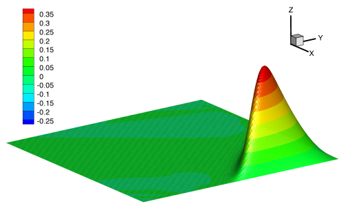
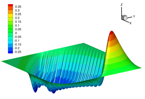
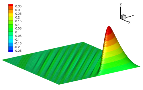
Figure 1. Numerical solution at $t=1$: DNS (top), POD-G model (2.7) (middle), and VMS-POD model (2.9) (bottom). Note that the VMS-POD model is much more accurate than the POD-G model, decreasing the unphysical oscillations of the latter. The CPU times for both the VMS-POD and POD-G models are three orders of magnitude lower than the CPU time for the DNS.

In conclusion, the VMS-POD model (2.9) dramatically decreases the error of the POD-G model (2.7) by adding numerical stabilization, while keeping the same level of computational efficiency.

Table 2. VMS-POD model’s average error $e=\frac{1}{N+1}{\sum\limits_{n=0}^{N}\|u^{n}-u_{r}^{n}\|}$ and its $e_{3}$ component for different values of $R$.

$R$	$e_{3}$	$\frac{1}{N+1}{\sum\limits_{n=0}^{N}\|u^{n}-u_{r}^{n}\|}$
1	1.29$\times 10^{-1}$	2.55$\times 10^{-2}$
4	9.34$\times 10^{-2}$	1.78$\times 10^{-2}$
7	6.69$\times 10^{-2}$	1.37$\times 10^{-2}$
10	4.68$\times 10^{-2}$	9.80$\times 10^{-3}$
13	3.20$\times 10^{-2}$	6.99$\times 10^{-3}$

We now turn our attention to the second major goal of this section - the numerical illustration of the theoretical error estimate (3.43). Specifically, we investigate whether the asymptotic behavior of the RHS of estimate (3.43) with respect to $R$ is reflected in the numerical results. We focus on the asymptotic behavior with respect to $R$ since this is the main parameter introduced by the VMS formulation; the asymptotic behavior with respect to $r$ was investigated in [7], whereas the asymptotic behavior with respect to $h$ and $\Delta t$ is standard [8, 39]. To investigate the asymptotic behavior with respect to $R$, we have to ensure that $\sqrt{\alpha}\sqrt{\sum\limits_{j=R+1}^{d}\lambda_{j}}$ (the only term that depends on $R$) dominates all the other terms on the RHS of (3.43). To this end, we start collecting all the terms that depend on the exact solution $u$ and we include them in the generic constant $C$. Next, we assume that the POD interpolation error in the initial condition $\|u^{0}-u_{r}^{0}\|$ is negligible. We also assume that the time-step is small enough to neglect $\Delta t\,\|u_{tt}\|_{L^{2}(L^{2})}$. With these assumptions, the error estimate (3.43) can now be written as $e\leq C\left(e_{1}+e_{2}+e_{3}\right)$, where $e$ is the VMS-POD model’s average error, $C$ a generic constant independent of $r,R,h,\Delta t$ and $\alpha$, $e_{1}=\|M_{r}^{-1}\|_{2}^{\frac{1}{2}}h^{m+1}$, $e_{2}=\|M_{r}^{-1}\|_{2}^{\frac{1}{2}}\sqrt{\sum\limits_{j=r+1}^{d}\lambda_{j}}$, and $e_{3}=\sqrt{\alpha}\sqrt{\sum\limits_{j=R+1}^{d}\lambda_{j}}$. To ensure that $e_{3}$ dominates the other terms, we choose $r=100$ and consider relatively low values for $R$. This choice for $r$, which is not optimal for practical computations, ensures, however, that $e_{3}$ dominates $e_{2}$. We also note that, when $h$ is small, $e_{3}$ dominates $e_{1}$ too. Thus, to investigate the asymptotic behavior with respect to $R$ of the RHS of (3.43), we fix $\alpha=5\times 10^{-3}$, vary $R$ from $1$ to $14$, and monitor the changes in $e_{3}$. We restrict $R$ to this parameter range to ensure that $\sqrt{\sum\limits_{j=R+1}^{d}\lambda_{j}}$ (and thus $e_{3}$) dominates $e_{2}$ and $e_{1}$. Table 2 lists the VMS-POD model’s average error $e=\frac{1}{N+1}{\sum\limits_{n=0}^{N}\|u^{n}-u_{r}^{n}\|}$ and its $e_{3}$ component for different values of $R$. We emphasize that, in this case, $e_{3}$ dominates the other two error components $e_{1}=3.81\times 10^{-3}$ and $e_{2}=2.87\times 10^{-3}$. To see whether the theoretical linear dependency predicted by the theoretical error estimate (3.43) is recovered in the numerical results in Table 2, we utilize a linear regression analysis in Figure 2. This plot shows that the rate of convergence of $e$ with respect to $e_{3}$ is $0.9$, which is close to the theoretical value of $1$ predicted by (3.43). We believe that this slight discrepancy is due to the fact that the mesh-size $h=0.01$ that we have employed in this numerical investigation is not small enough for our asymptotic study.

Summarizing the results above, we conclude that the theoretical error estimate in (3.43) is recovered asymptotically (with respect to $R$) in our numerical experiments.

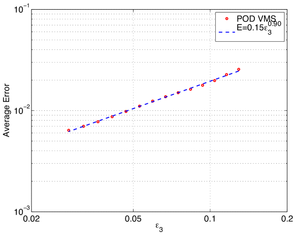
Figure 2. Linear regression of VMS-POD model’s average error with respect to $e_{3}$. The convergence rate is $0.9$, which is close to the theoretical value of $1$ predicted by (3.43).

Next, we use Theorem 3.5 to provide theoretical guidance in choosing an optimal value for the artificial viscosity coefficient $\alpha$. The main challenge is that the theoretical error estimate (3.43) is asymptotic with respect to $h,\Delta t$ and $r$, while in practical computations we are using small, yet non-negligible values for these parameters. Furthermore, the generic constant $C$ is problem-dependent and can play a significant role in practical computations. Notwithstanding these hurdles, we choose a value for $\alpha$ that minimizes the RHS of (3.43): $\widetilde{\alpha}=\frac{h^{m+1}+\sqrt{\sum\limits_{j=r+1}^{d}\lambda_{j}}}{2h^{m}+\sqrt{\sum\limits_{j=r+1}^{d}\lambda_{j}}+\sqrt{\sum\limits_{j=R+1}^{d}\lambda_{j}}}$. In the derivation of this formula, we made the same assumptions as those made in the numerical investigation of the asymptotic behavior of the VMS-POD model’s error and we again considered that (3.43) can be written as $e\leq C\left(e_{1}+e_{2}+e_{3}\right)$. We note that, if $\sqrt{\sum\limits_{j=r+1}^{d}\lambda_{j}}<<\sqrt{\sum\limits_{j=R+1}^{d}\lambda_{j}}$ and $h^{m}<<\sqrt{\sum\limits_{j=R+1}^{d}\lambda_{j}}$, then $\widetilde{\alpha}$ becomes too small in practical computations and the VMS-POD model becomes similar to the inaccurate POD-G model. To circumvent this, we use in our numerical tests a “clipping” procedure by setting $\alpha^{*}=\max\left\{\widetilde{\alpha},\frac{h}{2}\right\}$.

Table 3 lists the VMS-POD model’s average error $e=\frac{1}{N+1}{\sum\limits_{n=0}^{N}\|u^{n}-u_{r}^{n}\|}$ for the following values of $r,R$ and $\alpha$: $r=20,40$ and $60$; $R$ from $5$ to $r-5$ in increments of $5$; and $\alpha=0.01\,\alpha^{*},\,\alpha^{*}$, and $100\,\alpha^{*}$. Note that the VMS-POD model consistently performs best for $\alpha=\alpha^{*}$. The only two slight deviations from this rule are for $r=60$ ($R=20$ and $R=30$); we again believe that this is due to the mesh-size $h=0.01$, which is not small enough for the asymptotic regime in Theorem 3.5.

Table 3. VMS-POD model’s average error $e=\frac{1}{N+1}{\sum\limits_{n=0}^{N}\|u^{n}-u_{r}^{n}\|}$ for different values of $r$ and $R$, and $\alpha=0.01\,\alpha^{*},\,\alpha^{*}$, and $100\,\alpha^{*}$. Note that the VMS-POD model consistently performs best for $\alpha=\alpha^{*}$.

$r$	$R$	$0.01\alpha^{*}$	$e$	$\alpha^{*}$	$e$	$100\alpha^{*}$	$e$
20	5	$1.2\times 10^{-3}$	$1.0\times 10^{-1}$	$1.2\times 10^{-1}$	$5.8\times 10^{-2}$	$1.2\times 10^{1}$	$7.8\times 10^{-2}$
	10	$2.0\times 10^{-3}$	$9.5\times 10^{-2}$	$2.0\times 10^{-1}$	$2.4\times 10^{-2}$	$2.04\times 10^{1}$	$2.6\times 10^{-2}$
	15	$3.3\times 10^{-3}$	$8.2\times 10^{-2}$	$3.3\times 10^{-1}$	$2.0\times 10^{-2}$	$3.3\times 10^{1}$	$2.5\times 10^{-2}$
40	5	$6.4\times 10^{-5}$	$1.09\times 10^{-1}$	$6.4\times 10^{-3}$	$3.0\times 10^{-2}$	$6.4\times 10^{-1}$	$7.2\times 10^{-2}$
	10	$1.1\times 10^{-4}$	$1.0\times 10^{-1}$	$1.1\times 10^{-2}$	$1.8\times 10^{-2}$	$1.1\times 10^{0}$	$2.5\times 10^{-2}$
	20	$4.2\times 10^{-4}$	$9.7\times 10^{-2}$	$4.2\times 10^{-2}$	$4.4\times 10^{-3}$	$4.2\times 10^{0}$	$4.1\times 10^{-3}$
	30	$1.7\times 10^{-3}$	$6.8\times 10^{-2}$	$1.7\times 10^{-1}$	$8.1\times 10^{-3}$	$1.7\times 10^{1}$	$1.0\times 10^{-2}$
	35	$3.0\times 10^{-3}$	$4.9\times 10^{-2}$	$3.0\times 10^{-1}$	$2.1\times 10^{-2}$	$3.0\times 10^{1}$	$2.4\times 10^{-2}$
60	5	$5.0\times 10^{-5}$	$8.7\times 10^{-2}$	$5.0\times 10^{-3}$	$1.8\times 10^{-2}$	$5.0\times 10^{-1}$	$7.0\times 10^{-2}$
	10	$5.0\times 10^{-5}$	$8.7\times 10^{-2}$	$5.0\times 10^{-3}$	$1.3\times 10^{-2}$	$5.0\times 10^{-1}$	$2.4\times 10^{-2}$
	20	$5.0\times 10^{-5}$	$8.7\times 10^{-2}$	$5.0\times 10^{-3}$	$1.0\times 10^{-2}$	$5.0\times 10^{-1}$	$3.9\times 10^{-3}$
	30	$1.2\times 10^{-4}$	$8.0\times 10^{-2}$	$1.2\times 10^{-2}$	$4.4\times 10^{-3}$	$1.2\times 10^{0}$	$7.4\times 10^{-4}$
	40	$5.4\times 10^{-4}$	$5.5\times 10^{-2}$	$5.4\times 10^{-2}$	$1.2\times 10^{-3}$	$5.4\times 10^{0}$	$2.4\times 10^{-3}$
	50	$1.8\times 10^{-3}$	$2.6\times 10^{-2}$	$1.8\times 10^{-1}$	$1.3\times 10^{-2}$	$1.8\times 10^{1}$	$1.4\times 10^{-2}$
	55	$2.9\times 10^{-3}$	$2.2\times 10^{-2}$	$2.9\times 10^{-1}$	$1.1\times 10^{-2}$	$2.9\times 10^{1}$	$1.2\times 10^{-2}$

Finally, we investigate numerically the VMS-POD model’s sensitivity with respect to changes in the diffusion coefficient $\varepsilon$. To this end, we run the VMS-POD model (2.9) with the same parameters as above ($r=40,\,R=20$ and $\alpha=\alpha^{*}$) for different values of the diffusion coefficient: $\varepsilon=10^{-2},10^{-4}$ and $10^{-6}$. Table 4 lists the average errors for DNS, POD-G and VMS-POD models for different values of $\varepsilon$. It is clear from this table that the POD-G model’s average error is significantly higher than the error of the DNS. The VMS-POD model, however, performs well for all values of $\varepsilon$ and displays a low sensitivity with respect to changes in the diffusion coefficient. Thus, we provide numerical support for the theoretical estimate (3.43), which is uniform with respect to $\varepsilon$.

Table 4. Average errors of DNS, POD-G and VMS-POD models for different values of the diffusion coefficient $\varepsilon$. The POD-G model performs poorly. The VMS-POD model performs well and displays low sensitivity with respect to changes in $\varepsilon$.

$\varepsilon$	${DNS}$	POD-G	VMS-POD
	$\frac{1}{N+1}\sum\limits_{n=0}^{N}\|u^{n}-u_{h}^{N}\|$	$\frac{1}{N+1}{\sum\limits_{n=0}^{N}\|u^{n}-u_{r}^{n}\|}$	$\alpha$	$\frac{1}{N+1}{\sum\limits_{n=0}^{N}\|u^{n}-u_{r}^{n}\|}$
$10^{-2}$	$1.10\times 10^{-4}$	$1.10\times 10^{-2}$	$4.05\times 10^{-2}$	$4.27\times 10^{-3}$
$10^{-4}$	$2.04\times 10^{-4}$	$1.11\times 10^{-1}$	$4.29\times 10^{-2}$	$4.48\times 10^{-3}$
$10^{-6}$	$1.88\times 10^{-4}$	$1.17\times 10^{-1}$	$9.65\times 10^{-2}$	$4.05\times 10^{-3}$
$10^{-8}$	$2.46\times 10^{-4}$	$1.17\times 10^{-1}$	$1.01\times 10^{-1}$	$4.05\times 10^{-3}$

5. Conclusions

We presented a new VMS closure modeling strategy for the numerical stabilization of POD-ROMs of convection-dominated equations. The new POD-ROM, denoted VMS-POD, utilizes an artificial viscosity term to add numerical stabilization to the model. Following the guiding principle of the VMS methodology, we only add artificial viscosity to the small resolved scales. Thus, no artificial viscosity is used for the large resolved scales. The POD setting represents an ideal framework for the VMS approach, since the POD modes are listed in descending order of their kinetic energy content.

A thorough numerical analysis for the finite element discretization of the new VMS-POD model was presented. The numerical tests showed the increased numerical stability of the new VMS-POD model and illustrated the theoretical error estimates. We also employed the theoretical error estimates to provide guidance in choosing the artificial viscosity coefficient in practical computations. We emphasize that the theoretical error estimates were uniform with respect to $\varepsilon$, the diffusion coefficient. The numerical tests confirmed the theoretical results: The average error of the VMS-POD model showed a low sensitivity with respect to changes in $\varepsilon$.

Although the new VMS-POD model targets general convection-domainted problems, it was analyzed theoretically and tested numerically by using the convection-dominated convection-diffusion equations. We chose this simplified mathematical and numerical setting as a first step in a thorough investigation of the new VMS-POD model. Next, we will utilize the new VMS-POD model in the numerical simulation of turbulent flows, such as $3D$ flow past a circular cylinder [40]. We also note that, to our knowledge, this is the first time that the VMS formulation used in [29] for the numerical stabilization of finite element discretizations has been used in a POD setting. We will investigate in a future study the alternative VMS formulation proposed in [13] and compare it with the VMS-POD model that we introduced in this report.

References

• [1] N. Aubry, P. Holmes, J. L. Lumley, and E. Stone. The dynamics of coherent structures in the wall region of a turbulent boundary layer. J. Fluid Mech., 192:115–173, 1988.
• [2] N. Aubry, W. Y. Lian, and E. S. Titi. Preserving symmetries in the proper orthogonal decomposition. SIAM J. Sci. Comput., 14:483–505, 1993.
• [3] Y. Bazilevs, V. M. Calo, J. A. Cottrell, T. J. R. Hughes, A. Reali, and G. Scovazzi. Variational multiscale residual-based turbulence modeling for large eddy simulation of incompressible flows. Comput. Methods Appl. Mech. Engrg., 197(1-4):173–201, 2007.
• [4] M. Bergmann, C. H. Bruneau, and A. Iollo. Enablers for robust POD models. J. Comput. Phys., 228(2):516–538, 2009.
• [5] L. C. Berselli, T. Iliescu, and W. J. Layton. Mathematics of large eddy simulation of turbulent flows. Scientific Computation. Springer-Verlag, Berlin, 2006.
• [6] J. Borggaard, A. Duggleby, A. Hay, T. Iliescu, and Z. Wang. Reduced-order modeling of turbulent flows. In Proceedings of MTNS 2008, 2008.
• [7] J. Borggaard, T. Iliescu, and Z. Wang. Artificial viscosity proper orthogonal decomposition. Math. Comput. Modelling, 53(1-2):269–279, 2011.
• [8] S. C. Brenner and L. R. Scott. The mathematical theory of finite element methods, volume 15 of Texts in Applied Mathematics. Springer-Verlag, New York, 1994.
• [9] M. Buffoni, S. Camarri, A. Iollo, and M. V. Salvetti. Low-dimensional modelling of a confined three-dimensional wake flow. J. Fluid Mech., 569:141–150, 2006.
• [10] J. W. Demmel. Applied numerical linear algebra. Society for Industrial and Applied Mathematics Philadelphia, 1997.
• [11] V. Gravemeier. A consistent dynamic localization model for large eddy simulation of turbulent flows based on a variational formulation. J. Comput. Phys., 218(2):677–701, 2006.
• [12] V. Gravemeier, W. A. Wall, and E. Ramm. A three-level finite element method for the instationary incompressible Navier-Stokes equations. Comput. Methods Appl. Mech. Engrg., 193(15-16):1323–1366, 2004.
• [13] J.-L. Guermond. Stabilization of Galerkin approximations of transport equations by subgrid modeling. M2AN Math. Model. Numer. Anal., 33(6):1293–1316, 1999.
• [14] J.-L. Guermond. Stablisation par viscosité de sous-maille pour l’approximation de Galerkin des opérateurs linéaires monotones. C. R. Math. Acad. Sci. Paris, 328:617–622, 1999.
• [15] N. Heitmann. Subgridscale stabilization of time-dependent convection dominated diffusive transport. J. Math. Anal. Appl., 331(1):38–50, 2007.
• [16] P. Holmes, J. L. Lumley, and G. Berkooz. Turbulence, Coherent Structures, Dynamical Systems and Symmetry. Cambridge, 1996.
• [17] C. Homescu, L. R. Petzold, and R. Serban. Error estimation for reduced-order models of dynamical systems. SIAM J. Numer. Anal., 43(4):1693–1714 (electronic), 2005.
• [18] T. J. R. Hughes. Multiscale phenomena: Green’s functions, the Dirichlet-to-Neumann formulation, subgrid scale models, bubbles and the origins of stabilized methods. Comput. Methods Appl. Mech. Engrg., 127(1-4):387–401, 1995.
• [19] T. J. R. Hughes, L. Mazzei, and K. E. Jansen. Large eddy simulation and the variational multiscale method. Comput. Vis. Sci., 3:47–59, 2000.
• [20] T. J. R. Hughes, L. Mazzei, A. Oberai, and A. Wray. The multiscale formulation of large eddy simulation: Decay of homogeneous isotropic turbulence. Phys. Fluids, 13(2):505–512, 2001.
• [21] T. J. R. Hughes, A. Oberai, and L. Mazzei. Large eddy simulation of turbulent channel flows by the variational multiscale method. Phys. Fluids, 13(6):1784–1799, 2001.
• [22] V. John and S. Kaya. A finite element variational multiscale method for the Navier–Stokes equations. SIAM J. Sci. Comput., 26:1485, 2005.
• [23] V. John and S. Kaya. Finite element error analysis of a variational multiscale method for the Navier-Stokes equations. Adv. Comput. Math., 28(1):43–61, 2008.
• [24] V. John, S. Kaya, and A. Kindl. Finite element error analysis for a projection-based variational multiscale method with nonlinear eddy viscosity. J. Math. Anal. Appl., 344(2):627–641, 2008.
• [25] V. John, S. Kaya, and W. Layton. A two-level variational multiscale method for convection-dominated convection-diffusion equations. Comput. Methods Appl. Mech. Engrg., 195(33-36):4594–4603, 2006.
• [26] S. Kaya. Numerical analysis of a variational multiscale method for turbulence. PhD thesis, University of Pittsburgh, 2004.
• [27] K. Kunisch and S. Volkwein. Control of the Burgers equation by a reduced-order approach using proper orthogonal decomposition. J. Optim. Theory Appl., 102(2):345–371, 1999.
• [28] K. Kunisch and S. Volkwein. Galerkin proper orthogonal decomposition methods for parabolic problems. Numer. Math., 90(1):117–148, 2001.
• [29] W. J. Layton. A connection between subgrid scale eddy viscosity and mixed methods. Appl. Math. Comput., 133:147–157, 2002.
• [30] Z. Luo, J. Chen, I. M. Navon, and X. Yang. Mixed finite element formulation and error estimates based on proper orthogonal decomposition for the nonstationary Navier-Stokes equations. SIAM J. Numer. Anal., 47(1):1–19, 2008.
• [31] Z. D. Luo, J. Chen, P. Sun, and X. Z. Yang. Finite element formulation based on proper orthogonal decomposition for parabolic equations. Sci. China Ser. A, 52(3):585–596, 2009.
• [32] B. R. Noack, K. Afanasiev, M. Morzynski, G. Tadmor, and F. Thiele. A hierarchy of low-dimensional models for the transient and post-transient cylinder wake. J. Fluid Mech., 497:335–363, 2003.
• [33] B. Podvin. On the adequacy of the ten-dimensional model for the wall layer. Phys. Fluids, 13(1):210–224, 2001.
• [34] A. Quarteroni and A. Valli. Numerical approximation of partial differential equations. Springer Series in Computational Mathematics, 1994.
• [35] M. Schu and E. W. Sachs. Reduced order models in PIDE constrained optimization. Control Cybernet., 2010. to appear.
• [36] S. Sirisup and G. E. Karniadakis. A spectral viscosity method for correcting the long-term behavior of POD models. J. Comput. Phys., 194(1):92–116, 2004.
• [37] L. Sirovich. Turbulence and the dynamics of coherent structures. Parts I–III. Quart. Appl. Math., 45(3):561–590, 1987.
• [38] J. S. Smagorinsky. General circulation experiments with the primitive equations. Mon. Weather Review, 91:99–164, 1963.
• [39] V. Thomée. Galerkin finite element methods for parabolic problems. Springer Verlag, 2006.
• [40] Z. Wang, I. Akhtar, J. Borggaard, and T. Iliescu. Two-level discretizations of nonlinear closure models for proper orthogonal decomposition. J. Comput. Phys., 230:126–146, 2011.