What two models may teach us about duality violations in QCD

Abstract

Though the operator product expansion is applicable in the calculation of current correlation functions in the Euclidean region, when approaching the Minkowskian domain, violations of quark-hadron duality are expected to occur, due to the presence of bound-state or resonance poles. In QCD finite-energy sum rules, contour integrals in the complex energy plane down to the Minkowskian axis have to be performed, and thus the question arises what the impact of duality violations may be. The structure and possible relevance of duality violations is investigated on the basis of two models: the Coulomb system and a model for light-quark correlators which has already been studied previously. As might yet be naively expected, duality violations are in some sense “maximal” for zero-width bound states and they become weaker for broader resonances whose poles lie further away from the physical axis. Furthermore, to a certain extent, they can be suppressed by choosing appropriate weight functions in the finite-energy sum rules. A simplified Ansatz for including effects of duality violations in phenomenological QCD sum rule analyses is discussed as well.

1 Introduction

In phenomenological applications of QCD, the operator product expansion (OPE) wil69 ; wit77 plays an essential role. It is for example employed in applications of QCD sum rules svz79 or the analysis of the $\tau$ hadronic width bnp92 . Considering in particular two-point correlation functions of mesonic currents, strictly speaking the OPE is only appropriate in the Euclidean domain where $s\equiv q^{2}$ is sufficiently large and negative, with $q$ being the four-momentum transfer between the two currents. In the physical, Minkowskian domain with positive $s$, generally bound states or resonances are present which are governed by long-distance physics and which cannot be captured by a short-distance expansion.

In the Euclidean domain, a duality exists between descriptions of the system in terms of the quark and gluon degrees of freedom of QCD, or the physical hadronic degrees of freedom. Upon analytic continuation of correlation functions towards the Minkowskian region, due to the presence of bound-state poles, violations of the quark-hadron duality are expected to show up shi94 ; shi95 ; cdsu96 ; bsz98 . Since until now no analytic solution to QCD has been found – and it is unlikely that this will happen anytime soon – the precise functional form of duality violations (DVs) remains unknown. This necessitates to resort to the study of models in order to investigate their influence in phenomenological analyses of QCD. This is particularly pressing when employing so-called QCD finite-energy sum rules ckt78 ; kpt83 , because here contour integrals in the complex energy plane have to be computed down to the Minkowskian axis.

Based on the models presented in refs. shi94 ; shi95 ; bsz98 ; shi00 , the influence of duality violations on hadronic decays of the $\tau$ lepton has been investigated in recent years cgp05 ; cgp08 ; cgp09 ; gpp10a ; gpp10b , because they may play a role in precision determinations of fundamental QCD parameters, like the strong coupling $\alpha_{s}$ aleph05 ; bck08 ; bj08 ; ddhmz08 ; my08 . For example it has been observed that the compatibility of values for the gluon condensate $\langle\alpha_{s}GG\rangle$, extracted from fits to vector and axialvector $\tau$ decay spectra aleph05 ; ddhmz08 , is not very satisfactory. This poses the legitimate question if the inclusion of DVs in a consistent analysis may improve the situation regarding the compatibility of condensate parameters extracted from different channels, and in how far this would affect the resulting value of $\alpha_{s}$.

Though the particular model for vector and axialvector correlation functions employed in the analyses cgp05 ; cgp08 is based on features of large-$N_{c}$ QCD tho74 and Regge theory reg59 ; col71 , it is not directly rooted in fundamental QCD. Thus, it appears important to detect other systems which allow for an independent investigation of DVs, in particular their functional form as well as their possible impact on phenomenological analyses. A system that allows for an analytical treatment, and bears close relation to quarkonia in QCD in the limit of a heavy quark mass, is the Coulomb system. In the context of QCD moment sum rules, to some extent this example was already studied in ref. vol95 ; eid02 . Furthermore, in relation with hadronic decays of $B$ mesons, duality-violating contributions resulting from charmonium states were also considered in refs. bbns09 ; bbf11 .

In the first half of this article, it will be explored in more detail what can be learned from the Coulomb system regarding violations of duality. To this end, the notion of duality will be adopted in a more general context. The point of view taken in the following will be that a certain expansion is employed which in general can only be considered to be of an asymptotic nature. In our case this refers to the OPE, and duality is supposed to imply that the asymptotic expansion provides an acceptable representation of the full function. On the other hand, in some regions of the expansion, formally exponentially suppressed contributions may become relevant, and those will be identified with DVs.

One finding of the study of the Coulomb system below will be that due to the presence of zero-width bound-state poles on the real $s$-axis, the effects of DVs turn out to be particularly strong. The same conclusion has been drawn on the basis of the ‘t Hooft model mp09 . For this reason, the example of the Coulomb system will mainly be used to gain further general insights into the structure of DVs. For a more quantitative analysis, in the second half of this work recourse will again be taken to a simplified version of the model employed in refs. cgp05 ; cgp08 in the case of a finite width for the resonances. The finite width entails that the bound state poles move to the unphysical region of the complex $s$-plane and consequently, DVs in the physical region turn out to be less pronounced.

In refs. cgp08 ; cgp09 a simplified Ansatz was advocated in order to incorporate DV contributions into phenomenological QCD analyses. This Ansatz is supposed to be admissible if the resonances are sufficiently broad and thus lie sufficiently far away from the Minkowskian, physical axis. Towards the end of this article, arguments will be given why a related Ansatz should also be considered on an equal footing which is applicable in part of the complex energy plane, and the corresponding Ansatz is provided.

2 Sum rules for the Coulomb system

In the following, sum rules for the quantum mechanical Coulomb system will be set up, which are analogous to the sum rules studied in QCD svz79 . Quantum mechanical sum rules had already been investigated in the early years of QCD sum rules vzns80 ; bb81 ; nsvz81 ; pt84 , as analytical examples in which the techniques applied in QCD sum rule analysis could be studied and tested. Here, this route shall be followed for the question of duality violations.

Before going into the particular example of the Coulomb sum rule, let us set up the framework of quantum mechanical sum rules in more general terms pt84 . Consider a particle of mass $m$ under the influence of a potential $V(\vec{x})$. The Schrödinger equation for stationary states takes the form

$$\hat{H}\,\psi(\vec{x})\,\equiv\,\biggl{[}\,-\,\frac{\Delta}{2m}+V(\vec{x})\,\biggr{]}\psi(\vec{x})\;=\;E\,\psi(\vec{x})\,.$$ (1)

Let $\psi_{\alpha}(\vec{x})$ be the eigenfunction corresponding to the eigenvalue $E_{\alpha}$. The resolvent operator $\hat{G}(z)$ of $\hat{H}$ is defined as

$$\hat{G}(z)\,\equiv\,\Big{[}\,\hat{H}-z\hat{1}\,\Big{]}^{-1}\,,$$ (2)

where $z$ is an arbitrary complex number. Its matrix elements in the position representation are given by

$$G(\vec{x},\vec{y};z)\,\equiv\,\langle\vec{x}|\hat{G}(z)|\vec{y}\rangle\;=\;\sum\limits_{\alpha}\;\frac{\psi_{\alpha}(\vec{x})\psi_{\alpha}^{*}(\vec{y})}{(E_{\alpha}-z-i0)}+\int\frac{\rho_{\rm cont}(\vec{x},\vec{y};E)}{(E-z-i0)}\,{\rm d}E\,,$$ (3)

where the sum runs over the discrete spectrum, the integral is taken over the continuous spectrum and $\rho_{\rm cont}(\vec{x},\vec{y};E)$ is the spectral density corresponding to the continuous spectrum.

Let us introduce the function $D(E)$ which plays the analogous role of a physical correlation function in QCD sum rules, for example the Adler function adl74 :

$$D(E)\,\equiv\,\biggl{[}\,\frac{{\rm d}}{{\rm d}E}\,G(\vec{x},\vec{y};E)\,\biggr{]}_{\vec{x}=\vec{y}=0}\,.$$ (4)

Using eq. (3), $D(E)$ can be expressed as

$$D(E)\,=\,\sum\limits_{\alpha}\;\frac{|\psi_{\alpha}(0)|^{2}}{(E_{\alpha}-E-i0)^{2}}+\int\frac{\rho_{\rm cont}(E^{\prime})\,{\rm d}E^{\prime}}{(E^{\prime}-E-i0)^{2}}\,\equiv\,\int\frac{\rho(E^{\prime})\,{\rm d}E^{\prime}}{(E^{\prime}-E-i0)^{2}}\,,$$ (5)

with appropriate limits of integration, and where we furthermore have introduced the full spectral function

$$\rho(E)\,=\,\rho_{\rm pole}(E)+\rho_{\rm cont}(E)\,=\,\sum\limits_{\alpha}\,|\psi_{\alpha}(0)|^{2}\,\delta(E-E_{\alpha})+\rho_{\rm cont}(E)\,,$$ (6)

containing both the discrete as well as the continuous spectrum.

Let us now particularise the general expressions to the Coulomb problem. The ensuing sum rules turn out to be closely related to heavy-quark sum rules in QCD. Consider two particles of mass $m$ coupled by a Coulomb potential of the form

$$V(r)\,\equiv\,-\,\frac{\alpha}{r}\,.$$ (7)

The Coulomb potential is written with a general coupling $\alpha$, though one may well regard this as the leading term in the heavy-quark potential containing the QCD coupling $\alpha_{s}$. Solving the relevant Schrödinger equation, the radial Green function for the Coulomb potential is found to be vol95

$$G(r,0;E)\,=\,\frac{mk}{2\pi}\,e^{-kr}\,\Gamma(1-\lambda)\,U(1-\lambda,2;2kr)\,,$$ (8)

with

$$\lambda\,\equiv\,\frac{\alpha m}{2k}\qquad\mbox{and}\qquad k\;\equiv\;\sqrt{-\,m(E+i0)}\,.$$ (9)

$U(\alpha,\beta;z)$ is the confluent hypergeometric function. $G(r,0;E)$ is singular in the limit $r\rightarrow 0$, but the physical correlation function $D(E)$ remains finite and is found to be

$$D(E)\,\equiv\,\frac{{\rm d}}{{\rm d}E}\,G(r,0;E)\Big{|}_{r=0}\,=\,\frac{m\lambda}{4\pi\alpha}\Big{[}\,1+2\lambda+2\lambda^{2}\psi^{\prime}(1-\lambda)\,\Big{]}\,,$$ (10)

with $\psi(z)\equiv{\rm d}[\ln\Gamma(z)]/{\rm d}z$ being the logarithmic derivative of the Gamma function. The function $D(E)$ has poles at $\lambda_{n}=n$, $n=1,2,\ldots$ which translate to the bound-state energies $E_{n}$ of the Coulomb system with

$$E_{n}\,=\,-\,\frac{\alpha^{2}m}{4n^{2}}\,.$$ (11)

Expanding $D(E)$ around the position of the bound states, $E=E_{n}-\varepsilon$, from the leading $1/\varepsilon^{2}$ singularity the square of the wave function at the origin can be extracted,

$$|\psi_{n}(0)|^{2}\,=\,\frac{\alpha^{3}m^{3}}{8\pi n^{3}}\,,$$ (12)

which of course agrees with well known results in textbook quantum mechanics gp90 .

Besides the discrete spectrum for $E<0$, in the case of the Coulomb problem also a continuous spectrum is present for $E\geq 0$. Taking the imaginary part of eq. (3), one observes that the spectral density $\rho(E)$ is related to the imaginary part of $G(r,0;E)$, namely

$$\rho(E)\,=\,\frac{1}{\pi}\,\mbox{\rm Im}\,G(0,0;E+i0)\,.$$ (13)

Again, also $\mbox{\rm Im}\,G(r,0;E)$ is finite in the limit $r\rightarrow 0$ since it is a physical quantity. Calculating $\rho_{cont}(E)$ from eq. (10), yields

$$\rho_{cont}(E)\,=\,\frac{\alpha m^{2}}{4\pi\Big{[}1-e^{-\pi\alpha\sqrt{m/E}}\Big{]}}\,,\qquad E\,\geq\,0\,,$$ (14)

which is known as the so-called Sommerfeld factor som31 . Putting everything together, a finite-energy sum rule, analogous to the case of hadronic $\tau$ decays, for the quantum mechanical Coulomb problem can be written down:

$$R^{w}(E_{0})\,\equiv\,\int\limits_{E_{1}}^{E_{0}}w(E)\,\rho(E)\,{\rm d}E \,=\, \frac{i}{2\pi}\oint\limits_{E_{0}}w(E)\,G(0,0;E)\,{\rm d}E$$

$$\,=\, \frac{i}{2\pi}\oint\limits_{E_{0}}W(E)\,D(E)\,{\rm d}E\,,$$ (15)

which defines the moment $R^{w}(E_{0})$ corresponding to an arbitrary analytic weight function $w(E)$, and the weight function $W(E)$ is given by

$$W(E)\,=\,\int\limits_{E}^{E_{0}}w(E^{\prime})\,{\rm d}E^{\prime}\,.$$ (16)

The central idea of finite-energy sum rules is to employ a phenomenological representation of the spectral function $\rho(E)$ on the left-hand side of eq. (2) and a theoretically motivated, like the OPE, for $D(E)$ in the contour integral on the right-hand side. Equating both sides then allows to infer information on the physical spectrum from the theoretical description, or to extract theoretical parameters from the phenomenological information. As most probably in practical applications the theoretical expansion of $D(E)$ on the right-hand side is only of an asymptotic nature, the consequences for the finite-energy sum rule need to be investigated.

3 Asymptotic expansion and numerical analysis

For sufficiently large positive or negative energy $E$, that is $|\lambda|<1$, the $\psi^{\prime}$-function appearing in $D(E)$ of eq. (10) has a convergent expansion as72 . Therefore, in this energy region no duality violations are expected to occur. They may, however, arise in energy regions where $\psi^{\prime}(z)$ only has an asymptotic expansion, which is the case for $|z|=|1-\lambda|$ going to infinity, while $|\arg z|<\pi$. This happens if the energy is close to the continuum threshold $E=0$. In this region, the asymptotic expansion of $\psi^{\prime}(z)$ is given by as72

$$\psi^{\prime}(z)\,\sim\,\frac{1}{z}+\frac{1}{2z^{2}}+\sum\limits_{n=1}^{\infty}\frac{B_{2n}}{z^{2n+1}}\qquad(z\to\infty\;{\rm in}\;|\arg z|<\pi)\,,$$ (17)

where $B_{2n}$ are the Bernoulli numbers. Even though strictly speaking the asymptotic expansion (17) should be valid in the full region $|\arg z|<\pi$, due to the poles of $\psi(z)$ for $z=0,-1,-2,\ldots$, the asymptotic expansion becomes very inefficient if $z$ approaches these poles. Quite generally, in the left-half imaginary $z$-plane, that is $\mbox{\rm Re}\,z<0$, the asymptotic expansion can be greatly improved by applying the so-called reflection relation as72

$$\psi^{\prime}(z)\, = \,-\;\psi^{\prime}(-z)+\frac{1}{z^{2}}+\frac{\pi^{2}}{\sin^{2}(\pi z)}$$

$$\stackrel{{\scriptstyle z\to\infty}}{{\sim}} \,\frac{1}{z}+\frac{1}{2z^{2}}+\sum\limits_{n=1}^{\infty}\frac{B_{2n}}{z^{2n+1}}+\frac{\pi^{2}}{\sin^{2}(\pi z)}\qquad(\,\mbox{\rm Re}\,z<0\,)\,.$$ (18)

A more quantitative account on the improvement achieved by including the additional term in the expansion of (3) will be given in the second example of the next section.

As the asymptotic expansions of $\psi^{\prime}(z)$ and $-\,\psi^{\prime}(-z)+1/z^{2}$ are identical, it is clear that the additional term $\pi^{2}/\sin^{2}(\pi z)$ has to be exponentially suppressed. This can easily be verified by rewriting the $\sin$-function in terms of exponentials, which yields

$$\frac{\pi^{2}}{\sin^{2}(\pi z)}\,=\,-\,4\pi^{2}{\rm e}^{\pm 2\pi iz}+{\cal O}\left({\rm e}^{\pm 4\pi iz}\right)\qquad{\rm for}\;\;\mbox{\rm Im}\,z\!\!\phantom{x}^{>}_{<}\;0\,.$$ (19)

On the other hand, close to the poles of $\psi^{\prime}(z)$ the exponentially suppressed term provides an essential contribution as it gets enhanced by the poles contained in $1/\sin^{2}(\pi z)$ for $\mbox{\rm Im}\,z=0$. Thus, in the general terminology employed in the present work, the additional term (19) can be considered a duality-violating contribution.

In the following numerical analysis, the FESR (2) shall be investigated in a way such that the asymptotic expansion can be performed in a most transparent fashion. A convenient choice of the complex integration contour to this end are paths with constant $|1-\lambda|=|z|\equiv z_{0}$. The corresponding energy $E_{z}(\varphi)$ is then given by

$$E_{z}(\varphi)\,=\,-\,\frac{\alpha^{2}m}{4(z_{0}{\rm e}^{i\varphi}-1)^{2}}\,,$$ (20)

with the parametrisation $z=z_{0}\,{\rm e}^{i\varphi}$. Because of the square in the denominator, in the full range of $0<\varphi<2\pi$, the contour $E_{z}(\varphi)$ covers the complex $E$-plane twice. However, only the range $\varphi_{0}<\varphi<2\pi-\varphi_{0}$, where the angle $\varphi_{0}=\arccos(1/z_{0})$, and which contains the section on which the DV term (19) should be included in the asymptotic expansion of $\psi^{\prime}(z)$, provides the correct solution to the corresponding transcendental equation. Of particular interest are the two points

$$E_{0}\,\equiv\,E_{z}(\varphi_{0}) \,=\, \phantom{-}\,\frac{\alpha^{2}m}{4(z_{0}^{2}-1)}\,=\,\frac{-\,E_{1}}{(z_{0}^{2}-1)}\,,$$ (21)

$$\vbox{\vskip 22.76219pt}E_{\pi}\,\equiv\,E_{z}(\pi) \,=\, -\,\frac{\alpha^{2}m}{4(z_{0}+1)^{2}}\,=\,\frac{E_{1}}{(z_{0}+1)^{2}}\,,$$ (22)

where $E_{z}(\varphi)$ is real, and which have also been expressed in terms of the lowest-lying bound-state energy $E_{1}$. Eq. (22) shows that in order for the contour not to hit a bound-state pole, $z_{0}$ should not be integer, and that depending on $z_{0}$, poles with $n\geq{\rm int}(z_{0})+2$, where ${\rm int}(z_{0})$ denotes the integer part of $z_{0}$, need to be included on the phenomenological side of the sum rule, as they lie inside of the integration region.

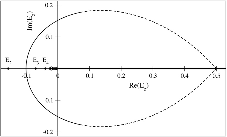
Figure 1: Integration contour $E_{z}(\varphi)$ in the complex $E$-plane for the FESR (2), employing $z_{0}=1.5$ and the further parameters provided in the text. The part of the contour where the DV term (19) should be included has been depicted as the solid line, and the remaining one, where the asymptotic expansion (17) is sufficient, as the dashed line. Some bound state poles as well as the continuum cut are also shown as thick dots and line, respectively.

As a particular example, the sum rule (2) will now be investigated numerically for the trivial weight function $w(E)=1$ and the set of parameters $\alpha=1/2$ and $m=10$. This leads to the lowest ground state being at $E_{1}=-5/8$. The integration contour in the $E$-plane is displayed in figure 1 for $z_{0}=1.5$, together with some bound state poles as well as the continuum cut (thick dots and line). The section on which $\psi^{\prime}(z)$ admits an asymptotic expansion without DV term is depicted as the dashed line, while the section where the DV term (19) should be included, is displayed as the solid line.

Next, figure 2 shows the moment $R^{w}(E_{0})$ of eq. (2) for the weight function $w(E)=1$, as a function of $z_{0}$. As expected, at the locations where $E_{z}(\pi)$ crosses a bound-state pole, $R^{w}(E_{0})$ is discontinuous. Employing the full Adler-type function $D(E)$ of eq. (10), it is a simple matter to verify that the equality between the phenomenological left-hand side of (2) in terms of $\rho(E)$ and the theoretical right-hand side is satisfied. On the other hand, when simulating the OPE with the asymptotic expansions (17) and (3) it is found that the DV term (19) completely dominates the moment. At the lowest considered $z_{0}=1.2$, the terms polynomial in $1/z$ only contribute about $0.3\,$% and at the highest plotted $z_{0}=5.5$, this contribution is within the numerical uncertainties of the asymptotic expansion. Hence, in the respective case, the moment $R^{w}(E_{0})$ is completely saturated by the DV contribution.

Figure 2: The solid line represents the moment $R^{w}(E_{0})$ of eq. (2) for the weight function $w(E)=1$, as a function of $z_{0}$. The discontinuities appear at the locations where the contour crosses a bound-state pole. The DV contribution (19) completely saturates this moment and is visually indistinguishable from the solid line.

There are two reasons that contribute to this behaviour. On the one hand, the Coulomb bound states are zero-width resonances and thus the duality violations are expected to be very strong. In such a case the DVs can be considered “maximal”. On the other hand, the weight function $w(E)=1$ does not provide any suppression of the resonance region which could soften the strong duality violations. The second issue can be investigated further by employing weight functions which provide some suppression of the resonance region, for example power-like moments $W^{(k)}(E)=(E-E_{\pi})^{k}(E-E_{0})$. Studying these weights for small $k=1,\,2,\,3$, it is found that indeed at low $z_{0}$ (close to the breakdown of the asymptotic expansion) the contribution of the DVs is suppressed. However, the dominance of DVs again quickly sets in for larger $z_{0}$, and even at low $z_{0}$ the contribution of DVs is still sizeable. The origin of the latter observation can be traced back to the fact that the DV term (19) penetrates some distance into the complex plane, before the exponential decay becomes effective. Thus, even with the weight functions $W^{(k)}(E)$, which nullify the contribution on the real axis, the residual contribution from the full contour integration can remain sizeable.

The dependence of the DVs on the resonance structure could be studied further by providing the Coulomb bound states with a finite width and varying this width. However, in view of practical applications of DV models in analyses of hadronic $\tau$ decays, the following discussion will be continued on the basis of a second model for DVs, already investigated in refs. shi00 ; cgp05 ; cgp08 .

4 A model for light-quark correlators

Following refs. shi00 ; cgp05 ; cgp08 , the structure of DVs shall be investigated in a second model, which incorporates constraints from Regge theory reg59 ; col71 on the light meson spectrum, and which can be chosen to roughly resemble the physical spectrum of the light-quark vector current correlator. The model employed below is a simplified version of the one studied in refs. cgp05 ; cgp08 , serving all purposes of the analysis discussed in the following. Specifically, it is chosen to take the form

$$\Pi_{V}(s)\,=\,-\;\psi\Biggl{(}\frac{M_{V}^{2}+u(s)}{\Lambda^{2}}\Biggr{)}+{\rm const.}\,,$$ (23)

where

$$u(s)\,=\,\Lambda^{2}\biggl{(}\frac{-s}{\Lambda^{2}}\biggr{)}^{\!\zeta}\qquad\mbox{and}\qquad\zeta\,=\,1-\frac{a}{\pi N_{c}}\,.$$ (24)

As compared to refs. cgp05 ; cgp08 , the lowest lying vector, that is the would-be $\rho$ meson, is included in the $\psi$-function. The reason for this will be explained below. Furthermore, in this work the global normalisation is immaterial and has been dropped. For all remaining parameters, in the numerical analysis numbers similar to the ones given in ref. cgp08 will be employed:

$$M_{V}\,=\,770\,\mbox{\rm MeV}\,,\qquad\Lambda\,=\,1.2\,\mbox{\rm GeV}\,,\qquad a\,=\,0.4\,.$$ (25)

In order to arrive at an OPE for the model, we require the expansion of the digamma function at large $|s|$, or correspondingly, large $|u|$. The expansion in question, which is however only asymptotic, takes the form as72

$$\psi(z)\,\sim\,\ln z-\frac{1}{2z}-\sum\limits_{n=1}^{\infty}\frac{B_{2n}}{2n\,z^{2n}}\qquad(z\to\infty\;{\rm in}\;|\arg z|<\pi)\,.$$ (26)

In fact, the asymptotic expansion of $\psi^{\prime}(z)$ of eq. (17) is of course just equal to the derivative of eq. (26). Though in principle one would have to further expand eq. (26) in terms of powers of $1/s$, in order to arrive at an OPE-like expansion, this is not necessary for what shall be discussed in the following, and thus we stick to the asymptotic expansion in powers of $1/z$.

For finite-width resonances, the poles are on an unphysical sheet, and $|\arg z|$ never reaches $\pi$. Still, like in the case of $\psi^{\prime}(z)$, in the region $\mbox{\rm Re}\,z<0$ the asymptotic expansion can be substantially improved by making use of the reflection relation cgp08 ; as72

$$\psi(z)\, = \,\psi(-z)-\frac{1}{z}-\pi\,\cot(\pi z)$$ (27)

$$\stackrel{{\scriptstyle z\to\infty}}{{\sim}} \,\ln z-\frac{1}{2z}-\sum\limits_{n=1}^{\infty}\frac{B_{2n}}{2n\,z^{2n}}-\pi\,[\,\cot(\pi z)\pm i\,]\quad(\,\mbox{\rm Re}\,z<0,\,\mbox{\rm Im}\,z^{\;>}_{\;<}\;0\,)\,.$$

Again, the logarithm and rational parts of both asymptotic expansions (26) and (27) agree, and it is a simple matter to convince oneself that away from the real axis the additional term $\pi\,[\,\cot(\pi z)\pm i\,]$ is exponentially suppressed, but takes once more care of the nearby poles.

Figure 3: $\mbox{\rm Re}[\psi(z)]$ (left pane) and $\mbox{\rm Im}[\psi(z)]$ (right pane), for $z=1.5\!\cdot\!\exp(i\varphi)$, as functions of $\varphi=\arg(z)$. The solid lines correspond to the full result, while the dashed lines show the asymptotic expansion of eq. (26), including terms up to $n=5$.

This is also demonstrated quantitatively in figure 3, where the real (left pane) and imaginary (right pane) parts of $\psi(z)$ are displayed for $z=1.5\!\cdot\!\exp(i\varphi)$ as functions of $\varphi=\arg(z)$. The solid lines correspond to the full function, while the dashed lines show the asymptotic expansion of eq. (26), including terms up to $n=5$. For positive real $z$ at this order the asymptotic series assumes its minimal term. As is evident, the asymptotic expansion breaks down for $\varphi~{}{}_{\textstyle\sim}^{\textstyle>}~{}2.5$. The difference between the total result and the asymptotic expansion is to a very good approximation covered by the additional term in eq. (27), such that taking this contribution into account, the quality of the expansion is analogous to the one for $\varphi<\pi/2$.

To continue, two finite-energy sum rules for the model (23) shall be investigated. For an arbitrary, analytic weight function $w(s)$, they take the generic form

$$R^{w}(s_{0})\,\equiv\,\int\limits_{0}^{s_{0}}\frac{{\rm d}s}{s_{0}}\,w(s)\,\rho_{V}(s)\,=\,\frac{i}{2\pi}\!\oint\limits_{s_{0}}\frac{{\rm d}s}{s_{0}}\,w(s)\,\Pi_{V}(s)\,,$$ (28)

where $\rho_{V}(s)\equiv\mbox{\rm Im}\,\Pi_{V}(s+i0)/\pi$, and the contour on the right-hand side is chosen such that it starts and ends at a real $s_{0}>0$.

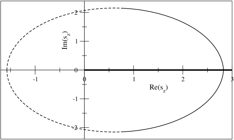
Figure 4: Integration contour $s_{z}(\varphi)$ of eq. (29) in the complex $s$-plane for the FESR (28), employing $z_{0}=1.5$ and the further parameters provided in the text. The part of the contour where the DV term should be included has been depicted as the solid line, and the remaining one as the dashed line. The cut of $\Pi_{V}(s)$ on the positive real $s$-axis is also indicated as the thick line.

The asymptotic expansion is again studied most cleanly for contours with constant absolute value of the argument of the $\psi$-function, $|z|=z_{0}$. The corresponding energy variable $s_{z}(\varphi)$ is then given by

$$s_{z}(\varphi)\,=\,-\,\Lambda^{2}\biggl{(}z_{0}\,{\rm e}^{i\varphi}-\frac{M_{V}^{2}}{\Lambda^{2}}\,\biggr{)}^{\!1/\zeta}\,,$$ (29)

and is displayed in figure 4 for the choice $z_{0}=1.5$. Again, the portion of the contour on which the DV term should be included is depicted as the solid line, while the remainder, on which the expansion (26) is admissible, is plotted as the dashed line. In order that the contour closes below the cut of $\Pi_{V}(s)$, that is $s_{z}(0)<0$, one requires $z_{0}>M_{V}^{2}/\Lambda^{2}\approx 0.41$. On the other hand this entails that $s_{0}~{}{}_{\textstyle\sim}^{\textstyle>}~{}1.2\,\mbox{\rm GeV}^{2}$. Because we have a model with finite-width resonances and the poles are located on an unphysical sheet, the angle $\varphi_{0}$ with $s_{z}(\varphi_{0})=s_{0}$ is found smaller than $\pi$. For example in the case of figure 4, in which $z_{0}=1.5$, $\varphi_{0}=2.972$. In the limit of zero-width resonances, corresponding to the large-$N_{c}$ limit, and which in the model (23) is realised as $\zeta\to 1$, $\varphi_{0}$ would go to $\pi$ and the poles would lie on the positive real $s$-axis. On the contrary, for broader resonances which lie further away from the real $s$-axis, the angle $\varphi_{0}$ is smaller, and the contribution of DVs gets reduced.

Figure 5: The solid line shows the moment $R^{w}(s_{0})$ of eq. (28) for the weight $w(s)=1$ and plotted as a function of $s_{0}$. The long- and short-dashed lines correspond to the power-like asymptotic expansion up to fourth and sixth order respectively.

The first example of a moment $R^{w}(s_{0})$ corresponding to eq. (28) is displayed in figure 5 for the trivial weight $w(s)=1$ and as a function of $s_{0}$. The oscillatory behaviour of the moment results from the presence of resonances, being damped for higher energies. As the long- and short-dashed lines, the asymptotic expansion (26) is plotted up to the fourth and sixth order in $z$ respectively. As is apparent, the asymptotic expansion breaks down at about $s_{0}\approx 1.5\,\mbox{\rm GeV}^{2}$. Furthermore, large deviations of the asymptotic expansion to the exact moment are observed, which are, however, perfectly described by the additional term in eq. (27). The largest deviation is found at the first minimum around $s_{0}\approx 1.76\,\mbox{\rm GeV}^{2}$, where the DVs amount to about $-11\%$ of the total contribution.

Figure 6: The solid line shows the moment $R^{w}(s_{0})$ of eq. (28) for the weight $w(s)=(1-s/s_{0})^{2}$ and plotted as a function of $s_{0}$. The long- and short-dashed lines correspond to the power-like asymptotic expansion up to fourth and sixth order respectively.

To investigate the influence of weight functions which provide some pinch suppression at $s=s_{0}$, in figure 6 the moment $R^{w}(s_{0})$ is displayed for the weight $w(s)=(1-s/s_{0})^{2}$, which has a double zero at $s=s_{0}$, just like the kinematical weight function in hadronic $\tau$ decays. Obviously, now the influence of DVs is much smaller though still clearly visible. At $s_{0}\approx 1.76\,\mbox{\rm GeV}^{2}$, the contribution of DVs amounts to only $1.6\%$ of the total moment, and a much stronger suppression is observed towards higher energies.

5 Conclusions

In phenomenological analyses of QCD, the operator product expansion is a widely used tool. While at sufficiently high energies the legitimacy of its application is unquestionable in the Euclidian domain, the continuation of the OPE towards the physical, Minkowskian region is inflicted with the appearance of duality violations. The presence of DV contributions, besides the OPE, is due to the physical bound states or resonances, whose physics cannot be captured by the OPE alone.

In the present article, the structure and impact of DVs has been studied on the basis of two models. Firstly, the quantum mechanical Coulomb system was investigated, which can serve as a model for heavy quarkonia, and which has not been considered in the context of finite-energy sum rules and DVs before. Secondly, a simplified version of a model already discussed extensively in refs. shi00 ; cgp05 ; cgp08 was used for comparison with the features found in the Coulomb model. The latter model incorporates constraints from large-$N_{c}$ QCD, as well as Regge theory, and captures the central features of the light-quark vector or axialvector correlators.

Qualitatively, the physical picture behind the appearance of duality violations can be summarised as follows: in the Euclidean region, all effects of resonances or bound-state poles have been sufficiently smoothed out, quark-hadron duality is expected to work well, and the OPE provides a satisfactory description of current correlation functions. When analytically continuing through the complex energy plane towards the physical, Minkowskian region, the presence of resonance poles becomes more and more prominent, reflecting itself in a breakdown of the OPE. Mathematically, the DV contributions show up as formally exponentially suppressed terms in an asymptotic expansion, which are, however, enhanced by the nearby poles, and thus can become numerically relevant.

The strength of effects resulting from DVs can be considered “maximal” if the bound states have zero width and the poles lie on the Minkowskian axis. This case is for example realised in the Coulomb model or when $N_{c}$ in eq. (24) of the second model is taken to infinity cgp05 . On the other hand, the influence of DVs is suppressed for resonances with a finite width and becomes smaller when the resonances are broader and the poles lie further away from the physical, Minkowskian axis. This is also seen from the oscillations in the physical spectrum whose features cannot be described adequately by the OPE. These oscillations are more prominent for narrower resonances while they become weaker if the resonances get broader.

If the physical resonances are sufficiently broad, and thus lie sufficiently far away from the physical axis, a simplified description of DVs as an exponentially damped oscillatory function appears admissible. Assuming $s$ to be large enough for the OPE to make sense, motivated by the $\psi$-function model such a simplified Ansatz was advocated in refs. cgp08 ; cgp09 for the duality violating spectral function $\rho_{\rm DV}(s)$ in the form

$$\rho_{\rm DV}(s)\,=\,\kappa\,{\rm e}^{-\gamma s}\sin(\alpha+\beta s)\,,$$ (30)

where $\kappa$, $\gamma$, $\alpha$ and $\beta$ are a priori free parameters which in a specific channel have to be extracted from experiment, and which bear no immediate QCD interpretation. The DV contribution to a moment is then assumed to be given by

$$R^{w}_{\rm DV}(s_{0})\,=\,-\!\int\limits_{s_{0}}^{\infty}\frac{{\rm d}s}{s_{0}}\,w(s)\,\rho_{\rm DV}(s)\,.$$ (31)

In practical applications of QCD finite-energy sum rules, however, the DVs naturally are required on the complex contour and thus a closely related Ansatz, which corresponds to the continuation of eq. (30) to the right complex half-plane, may also be considered:

$$\Pi_{\rm DV}(s)\,=\,\pi\,\kappa\,{\rm e}^{-\,\gamma s\,\pm\,i\,(\alpha+\beta s)}\qquad(\,\mbox{\rm Re}\,s>0,\,\mbox{\rm Im}\,s^{\;>}_{\;<}\;0\,)\,,$$ (32)

with $\gamma$ and $\beta$ positive. Of course, the $\mbox{\rm Im}\,\Pi_{\rm DV}(s)$ on the positive, real $s$-axis reproduces the spectrum of eq. (30), but the Ansatz also reflects the form of the exponential suppression of the DV term given in eq. (19). Both Ansätze (30) and (32) would be totally equivalent, if the DV contribution would be active on all of the complex contour. However, since the DV term should only be included on part of the contour (the solid-line sections in figures 1 and 4, or, more generically, on the right-half $s$-plane $\mbox{\rm Re}\,s>0$), both choices differ by an exponentially suppressed contribution. As a matter of principle this should be numerically irrelevant, but it could play a certain role if in practical applications the exponential suppression is not very pronounced. This will be studied in the future in investigations like the ones of refs. cgp09 ; bcgjmop10 .

To conclude, in the presented article observations about duality violations appearing in asymptotic expansions were summarised on the basis of two models. One of them has already been discussed in the literature before, while the other, the Coulomb system, has not been studied with respect to DVs previously. The qualitative findings of this work should prove useful for phenomenological QCD studies in the future.

- (1) K. G. Wilson, Non-Lagrangian models of current algebra, Phys. Rev. 179 (1969) 1499–1512.
- (2) E. Witten, Short distance analysis of weak interactions, Nucl. Phys. B122 (1977) 109.
- (3) M. A. Shifman, A. I. Vainshtein, and V. I. Zakharov, QCD and resonance physics: Sum Rules, Nucl. Phys. B147 (1979) 385, 448.
- (4) E. Braaten, S. Narison, and A. Pich, QCD analysis of the hadronic width, Nucl. Phys. B373 (1992) 581–612.
- (5) M. A. Shifman, Theory of pre-asymptotic effects in weak inclusive decays, hep-ph/9405246. In Proc. of the Workshop Continuous advances in QCD, ed. A. Smilga (World Scientific, Singapore, 1994).
- (6) M. A. Shifman, Recent progress in the heavy quark theory, hep-ph/9505289. In Particles, Strings and Cosmology, eds. J. Bagger et al. (World Scientific, Singapore, 1996).
- (7) B. Chibisov, R. D. Dikeman, M. A. Shifman, and N. Uraltsev, Operator product expansion, heavy quarks, QCD duality and its violations, Int. J. Mod. Phys. A12 (1997) 2075–2133, [hep-ph/9605465].
- (8) B. Blok, M. A. Shifman, and D.-X. Zhang, An Illustrative example of how quark hadron duality might work, Phys. Rev. D57 (1998) 2691–2700, [hep-ph/9709333].
- (9) M. A. Shifman, Quark-hadron duality, hep-ph/0009131. Published in the Boris Ioffe Festschrift ’At the Frontier of Particle Physics / Handbook of QCD’, ed. M. Shifman (World Scientific, Singapore, 2001).
- (10) K. G. Chetyrkin, N. V. Krasnikov, and A. N. Tavkhelidze, Finite energy sum rules for the cross-section of annihilation into hadrons in QCD, Phys. Lett. B76 (1978) 83–84.
- (11) N. V. Krasnikov, A. A. Pivovarov, and N. N. Tavkhelidze, The use of finite energy sum rules for the description of the hadronic properties of QCD, Z. Phys. C19 (1983) 301.
- (12) O. Catà, M. Golterman, and S. Peris, Duality violations and spectral sum rules, JHEP 0508 (2005) 076, [hep-ph/0506004].
- (13) O. Catà, M. Golterman, and S. Peris, Unraveling duality violations in hadronic decays, Phys. Rev. D77 (2008) 093006, [arXiv:0803.0246].
- (14) O. Catà, M. Golterman, and S. Peris, Possible duality violations in decay and their impact on the determination of , Phys. Rev. D79 (2009) 053002, [arXiv:0812.2285].
- (15) M. Gonzalez-Alonso, A. Pich, and J. Prades, Violation of quark-hadron duality and spectral chiral moments in QCD, Phys. Rev. D81 (2010) 074007, [arXiv:1001.2269].
- (16) M. Gonzalez-Alonso, A. Pich, and J. Prades, Pinched weights and duality violation in QCD sum rules: a critical analysis, Phys. Rev. D82 (2010) 014019, [arXiv:1004.4987].
- (17) ALEPH Collaboration, S. Schael et. al., Branching ratios and spectral functions of decays: Final ALEPH measurements and physics implications, Phys. Rept. 421 (2005) 191–284, [hep-ex/0506072].
- (18) P. A. Baikov, K. G. Chetyrkin, and J. H. Kühn, Order QCD corrections to and decays, Phys. Rev. Lett. 101 (2008) 012002, [arXiv:0801.1821].
- (19) M. Beneke and M. Jamin, and the hadronic width: fixed-order, contour-improved and higher-order perturbation theory, JHEP 0809 (2008) 044, [arXiv:0806.3156].
- (20) M. Davier, S. Descotes-Genon, A. Höcker, B. Malaescu, and Z. Zhang, The determination of from decays revisited, Eur. Phys. J. C56 (2008) 305–322, [arXiv:0803.0979].
- (21) K. Maltman and T. Yavin, from hadronic decays, Phys. Rev. D78 (2008) 094020, [arXiv:0807.0650].
- (22) G. ’t Hooft, A planar diagram theory for strong interactions, Nucl. Phys. B72 (1974) 461.
- (23) T. Regge, Introduction to complex orbital momenta, Nuovo Cim. 14 (1959) 951.
- (24) P. D. B. Collins, Regge theory and particle physics, Phys. Rept. 1 (1971) 103–234.
- (25) M. B. Voloshin, Precision determination of and from QCD sum rules for , Int. J. Mod. Phys. A10 (1995) 2865–2880, [hep-ph/9502224].
- (26) M. Eidemüller, QCD moment sum rules for Coulomb systems: The charm and bottom quark masses, Phys. Rev. D67 (2003) 113002, [hep-ph/0207237].
- (27) M. Beneke, G. Buchalla, M. Neubert, and C. T. Sachrajda, Penguins with charm and quark-hadron duality, Eur. Phys. J. C61 (2009) 439–449, [arXiv:0902.4446].
- (28) M. Beylich, G. Buchalla, and T. Feldmann, Theory of decays at high : OPE and quark-hadron duality, arXiv:1101.5118.
- (29) J. Mondejar and A. Pineda, Deep inelastic scattering and factorization in the ’t Hooft Model, Phys. Rev. D79 (2009) 085011, [arXiv:0901.3113].
- (30) A. I. Vainshtein, V. I. Zakharov, V. A. Novikov, and M. A. Shifman, Asymptotic freedom in quantum mechanics, Sov. J. Nucl. Phys. 32 (1980) 840.
- (31) J. S. Bell and R. A. Bertlmann, MAGIC moments, Nucl. Phys. B177 (1981) 218.
- (32) V. A. Novikov, M. A. Shifman, A. I. Vainshtein, and V. I. Zakharov, Are all hadrons alike?, Nucl. Phys. B191 (1981) 301.
- (33) P. Pascual and R. Tarrach, QCD: Renormalization for the Practitioner. Lecture Notes in Physics 194, Springer-Verlag, 1984.
- (34) S. L. Adler, Some simple vacuum polarization phenomenology: Hadrons, Phys. Rev. D10 (1974) 3714.
- (35) K. Melnikov and A. Yelkhovsky, The -quark low-scale running mass from Upsilon sum rules, Phys. Rev. D59 (1999) 114009, [hep-ph/9805270].
- (36) A. Galindo and P. Pascual, Quantum Mechanics I. Springer-Verlag, 1990.
- (37) A. Sommerfeld, Über die Beugung und Bremsung der Elektronen, Ann. Phys. 403 (1931) 257.
- (38) M. Abramowitz and I. A. Stegun, Handbook of Mathematical Functions. Dover Publications, 1972.
- (39) R. B. Dingle, Asymptotic Expansions: Their Derivation and Interpretation. Academic Press, 1973.
- (40) R. B. Paris and D. Kaminski, Asymptotics and Mellin-Barnes Integrals. Cambridge University Press, 2001.
- (41) D. R. Boito, O. Catà, M. Golterman, M. Jamin, K. Maltman, J. Osborne, and S. Peris, Duality violations in hadronic spectral moments, arXiv:1011.4426. To appear in Proc. of Tau2010, Manchester, UK.