Bayesian inverse problems with Gaussian priors

Abstract

The posterior distribution in a nonparametric inverse problem is shown to contract to the true parameter at a rate that depends on the smoothness of the parameter, and the smoothness and scale of the prior. Correct combinations of these characteristics lead to the minimax rate. The frequentist coverage of credible sets is shown to depend on the combination of prior and true parameter, with smoother priors leading to zero coverage and rougher priors to conservative coverage. In the latter case credible sets are of the correct order of magnitude. The results are numerically illustrated by the problem of recovering a function from observation of a noisy version of its primitive.

, and

t1Supported in part by the Netherlands Organization for Scientific Research NWO.

1 Introduction

In this paper we study a Bayesian approach to estimating a parameter ${\mu}$ from an observation $Y$ following the model

$$Y=K{\mu}+\frac{1}{\sqrt{n}}Z.$$ (1)

The unknown parameter ${\mu}$ is an element of a separable Hilbert space $H_{1}$, and is mapped into another Hilbert space $H_{2}$ by a known, injective, continuous linear operator $K\dvtx H_{1}\to H_{2}$. The image $K{\mu}$ is perturbed by unobserved, scaled Gaussian white noise $Z$. There are many special examples of this infinite-dimensional regression model, which can also be viewed as an idealized version of other statistical models, including density estimation. The inverse problem of estimating ${\mu}$ has been studied by both statisticians and numerical mathematicians (see, e.g., Donoho , Cavalier , Munk , RuymgaartII , RuymgaartIII , Stuart for reviews), but rarely from a theoretical Bayesian perspective; exceptions are Cox and Simoni .

The Bayesian approach to (1) consists of putting a prior on the parameter ${\mu}$, and computing the posterior distribution. We study Gaussian priors, which are conjugate to the model, so that the posterior distribution is also Gaussian and easy to derive. Our interest is in studying the properties of this posterior distribution, under the “frequentist” assumption that the data $Y$ has been generated according to the model (1) with a given “true” parameter ${\mu}_{0}$. We investigate whether and at what rate the posterior distributions contract to ${\mu}_{0}$ as $n\rightarrow\infty$ (as in GGvdV ), but have as main interest the performance of credible sets for measuring the uncertainty about the parameter.

A Bayesian credible set is defined as a central region in the posterior distribution of specified posterior probability, for instance, 95%. As a consequence of the Bernstein–von Mises theorem credible sets for smooth finite-dimensional parametric models are asymptotically equivalent to confidence regions based on the maximum likelihood estimator (see, e.g., vdVAS , Chapter 10), under mild conditions on the prior. Thus, “Bayesian uncertainty” is equivalent to “frequentist uncertainty” in these cases, at least for large $n$. However, there is no corresponding Bernstein–von Mises theorem in nonparametric Bayesian inference, as noted in Freedman . The performance of Bayesian credible sets in these situations has received little attention, although in practice such sets are typically provided as indicators of uncertainty, for instance, based on the spread of the output of a (converged) MCMC run. The paper Cox did tackle this issue and came to the alarming conclusion that Bayesian credible sets have frequentist coverage zero. If this were true, many data analysts would (justifiably) distrust the spread in the posterior distribution as a measure of uncertainty. For other results see Bontemps , Ghosal99 , Ghosal00 and Leahu .

The model considered in Cox is equivalent to our model (1), and a good starting point for studying these issues. More precisely, the conclusion of Cox is that for almost every parameter ${\mu}_{0}$ from the prior the coverage of a credible set (of any level) is 0. In the present paper we show that this is only part of the story, and, taken by itself, the conclusion is misleading. The coverage depends on the true parameter ${\mu}_{0}$ and the prior together, and it can be understood in terms of a bias-variance trade-off, much as the coverage of frequentist nonparametric procedures. A nonparametric procedure that oversmoothes the truth (too big a bandwidth in a frequentist procedure, or a prior that puts too much weight on “smooth” parameters) will be biased, and a confidence or credible region based on such a procedure will be both too concentrated and wrongly located, giving zero coverage. On the other hand, undersmoothing does work (to a certain extent), also in the Bayesian setup, as we show below. In this light we reinterpret the conclusion of Cox to be valid only in the oversmoothed case (notwithstanding a conjecture to the contrary in the Introduction of this paper; see page 905, answer to objection 4). In the undersmoothed case credible regions are conservative in general, with coverage tending to 1. The good news is that typically they are of the correct order of magnitude, so that they do give a reasonable idea of the uncertainty in the estimate.

Of course, whether a prior under- or oversmoothes depends on the regularity of the true parameter. In practice, we may not want to consider this known, and adapt the prior smoothness to the data. In this paper we do consider the effect of changing the “length scale” of a prior, but do not study data-dependent length scales. The effect of setting the latter by, for example, an empirical or full Bayes method will require further study.

Credible sets are by definition “central regions” in the posterior distribution. Because the posterior distribution is a random probability measure on the Hilbert space $H_{1}$, a “central ball” is a natural shape of such a set, but it has the disadvantage that it is difficult to visualize. If the Hilbert space is a function space, then credible bands are more natural. These correspond to simultaneous credible intervals for the function at a point, and can be obtained from the (marginal) posterior distributions of a set of linear functionals. Besides the full posterior distribution, we therefore study its marginals for linear functionals. The same issue of the dependence of coverage on under- and oversmoothing arises, except that “very smooth” linear functionals cancel the inverse nature of the problem, and do allow a Bernstein–von Mises theorem for a large set of priors. Unfortunately point evaluations are usually not smooth in this sense.

Thus, we study two aspects of inverse problems—recovering the full parameter ${\mu}$ (Section 4) and recovering linear functionals (Section 5). We obtain the rate of contraction of the posterior distribution in both settings, in its dependence on parameters of the prior. Furthermore, and most importantly, we study the “frequentist” coverage of credible regions for ${\mu}$ in both settings, for the same set of priors. In the next section we give a more precise statement of the problem, and in Section 3 we describe the priors that we consider and derive the corresponding posterior distributions. In Section 6 we illustrate the results by simulations and pictures in the particular example that $K$ is the Volterra operator. Technical proofs are placed in Sections 7 and 8 at the end of the paper.

Throughout the paper $\langle\cdot,\cdot\rangle_{1}$ and $\|\cdot\|_{1}$, and $\langle\cdot,\cdot\rangle_{2}$ and $\|\cdot\|_{2}$ denote the inner products and norms of the Hilbert spaces $H_{1}$ and $H_{2}$. The adjoint of an operator $A$ between two Hilbert spaces is denoted by $A^{T}$. The Sobolev space $S^{\beta}$ with its norm $\|\cdot\|_{\beta}$ is defined in (3). For two sequences $(a_{n})$ and $(b_{n})$ of numbers $a_{n}\asymp b_{n}$ means that $|a_{n}/b_{n}|$ is bounded away from zero and infinity as $n\rightarrow\infty$, and $a_{n}\lesssim b_{n}$ means that $a_{n}/b_{n}$ is bounded.

2 Detailed description of the problem

The noise process $Z$ in (1) is the standard normal or iso-Gaussian process for the Hilbert space $H_{2}$. Because this is not realizable as a random element in $H_{2}$, the model (1) is interpreted in process form (as in Munk ). The iso-Gaussian process is the zero-mean Gaussian process $Z=(Z_{h}\dvtx h\in H_{2})$ with covariance function $\mathrm{E}Z_{h}Z_{h^{\prime}}=\langle h,h^{\prime}\rangle_{2}$, and the measurement equation (1) is interpreted in that we observe a Gaussian process $Y=(Y_{h}\dvtx h\in H_{2})$ with mean and covariance functions

$$\mathrm{E}Y_{h}=\langle K{\mu},h\rangle_{2},\qquad\operatorname{cov}(Y_{h},Y_{h^{\prime}})=\frac{1}{n}\langle h,h^{\prime}\rangle_{2}.$$ (2)

Sufficiency considerations show that it is statistically equivalent to observe the subprocess $(Y_{h_{i}}\dvtx i\in\mathbb{N})$, for any orthonormal basis $h_{1},h_{2},\ldots$ of $H_{2}$.

If the operator $K$ is compact, then the spectral decomposition of the self-adjoint operator $K^{T}K\dvtx H_{1}\to H_{1}$ provides a convenient basis. In the compact case the operator $K^{T}K$ possesses countably many positive eigenvalues ${\kappa}_{i}^{2}$ and there is a corresponding orthonormal basis $(e_{i})$ of $H_{1}$ of eigenfunctions (hence, $K^{T}Ke_{i}={\kappa}_{i}^{2}e_{i}$ for $i\in\mathbb{N}$; see, e.g., Rudin ). The sequence $(f_{i})$ defined by $Ke_{i}={\kappa}_{i}f_{i}$ forms an orthonormal “conjugate” basis of the range of $K$ in $H_{2}$. An element ${\mu}\in H_{1}$ can be identified with its sequence $({\mu}_{i})$ of coordinates relative to the eigenbasis $(e_{i})$, and its image $K{\mu}=\sum_{i}{\mu}_{i}Ke_{i}=\sum_{i}\mu_{i}{\kappa}_{i}f_{i}$ can be identified with its coordinates $({\mu}_{i}{\kappa}_{i})$ relative to the conjugate basis $(f_{i})$. If we write $Y_{i}$ for $Y_{f_{i}}$, then (2) shows that $Y_{1},Y_{2},\ldots$ are independent Gaussian variables with means $\mathrm{E}Y_{i}=\mu_{i}{\kappa}_{i}$ and variance $1/n$. Therefore, a concrete equivalent description of the statistical problem is to recover the sequence $({\mu}_{i})$ from independent observations $Y_{1},Y_{2},\ldots$ with $N(\mu_{i}{\kappa}_{i},1/n)$-distributions.

In the following we do not require $K$ to be compact, but we do assume the existence of an orthonormal basis of eigenfunctions of $K^{T}K$. The main additional example we then cover is the white noise model, in which $K$ is the identity operator. The description of the problem remains the same.

If ${\kappa}_{i}\rightarrow 0$, this problem is ill-posed, and the recovery of ${\mu}$ from $Y$ an inverse problem. The ill-posedness can be quantified by the speed of decay ${\kappa}_{i}\downarrow 0$. Although the tools are more widely applicable, we limit ourselves to the mildly ill-posed problem (in the terminology of Cavalier ) and assume that the decay is polynomial: for some $p\geq 0$,

$${\kappa}_{i}\asymp i^{-p}.$$

Estimation of ${\mu}$ is harder if the decay is faster (i.e., $p$ is larger).

The difficulty of estimation may be measured by the minimax risks over the scale of Sobolev spaces relative to the orthonormal basis $(e_{i})$ of eigenfunctions of $K^{T}K$. For ${\beta}>0$ define

$$\|{\mu}\|_{\beta}=\sqrt{\sum_{i=1}^{\infty}{\mu}_{i}^{2}i^{2{\beta}}}\qquad\mbox{if }{\mu}=\sum_{i=1}^{\infty}{\mu}_{i}e_{i}.$$ (3)

Then the Sobolev space of order ${\beta}$ is $S^{\beta}=\{{\mu}\in H_{1}\dvtx\|{\mu}\|_{\beta}<\infty\}$. The minimax rate of estimation over the unit ball of this space relative to the loss $\|t-{\mu}\|_{1}$ of an estimate $t$ for ${\mu}$ is $n^{-{\beta}/(1+2{\beta}+2p)}$. This rate is attained by various “regularization” methods, such as generalized Tikhonov and Moore–Penrose regularization Mair , Bertero , Cavalier , Goldenshluger , Munk . The Bayesian approach is closely connected to these methods: in Section 3 the posterior mean is shown to be a regularized estimator.

Besides recovery of the full parameter ${\mu}$, we consider estimating linear functionals $L{\mu}$. The minimax rate for such functionals over Sobolev balls depends on $L$ as well as on the parameter of the Sobolev space. Decay of the coefficients of $L$ in the eigenbasis may alleviate the level of ill-posedness, with rapid decay even bringing the functional in the domain of “regular” $n^{-1/2}$-rate estimation.

3 Prior and posterior distributions

We assume a mean-zero Gaussian prior for the parameter ${\mu}$. In the next three paragraphs we recall some essential facts on Gaussian distributions on Hilbert spaces.

A Gaussian distribution $N({\nu},\Lambda)$ on the Borel sets of the Hilbert space $H_{1}$ is characterized by a mean ${\nu}$, which can be any element of $H_{1}$, and a covariance operator $\Lambda\dvtx H_{1}\to H_{1}$, which is a nonnegative-definite, self-adjoint, linear operator of trace class: a compact operator with eigenvalues $({\lambda}_{i})$ that are summable $\sum_{i=1}^{\infty}{\lambda}_{i}<\infty$ (see, e.g., Skorohod , pages 18–20). A random element $G$ in $H_{1}$ is $N({\nu},\Lambda)$-distributed if and only if the stochastic process $(\langle G,h\rangle_{1}\dvtx h\in H_{1})$ is a Gaussian process with mean and covariance functions

$$\mathrm{E}\langle G,h\rangle_{1}=\langle{\nu},h\rangle_{1},\qquad\operatorname{cov}(\langle G,h\rangle_{1},\langle G,h^{\prime}\rangle_{1})=\langle h,\Lambda h^{\prime}\rangle_{1}.$$ (4)

The coefficients $G_{i}=\langle G,\varphi_{i}\rangle_{1}$ of $G$ relative to an orthonormal eigenbasis $(\varphi_{i})$ of $\Lambda$ are independent, univariate Gaussians with means the coordinates $({\nu}_{i})$ of the mean vector ${\nu}$ and variances the eigenvalues ${\lambda}_{i}$.

The iso-Gaussian process $Z$ in (1) may be thought of as a $N(0,I)$-distributed Gaussian element, for $I$ the identity operator (on $H_{2}$), but as $I$ is not of trace class, this distribution is not realizable as a proper random element in $H_{2}$. Similarly, the data $Y$ in (1) can be described as having a $N(K{\mu},n^{-1}I)$-distribution.

For a stochastic process $W=(W_{h}\dvtx h\in H_{2})$ and a continuous, linear operator $A\dvtx H_{2}\to H_{1}$, we define the transformation $AW$ as the stochastic process with coordinates $(AW)_{h}=W_{A^{T}h}$, for $h\in H_{1}$. If the process $W$ arises as $W_{h}=\langle W,h\rangle_{2}$ from a random element $W$ in the Hilbert space $H_{2}$, then this definition is consistent with identifying the random element $AW$ in $H_{1}$ with the process $(\langle AW,h\rangle_{1}\dvtx h\in H_{1})$, as in (4) with $G=AW$. Furthermore, if $A$ is a Hilbert–Schmidt operator (i.e., $AA^{T}$ is of trace class), and $W=Z$ is the iso-Gaussian process, then the process $AW$ can be realized as a random variable in $H_{1}$ with a $N(0,AA^{T})$-distribution.

In the Bayesian setup the prior, which we take $N(0,\Lambda)$, is the marginal distribution of $\mu$, and the noise $Z$ in (1) is considered independent of ${\mu}$. The joint distribution of $(Y,{\mu})$ is then also Gaussian, and so is the conditional distribution of ${\mu}$ given $Y$, the posterior distribution of ${\mu}$. In general, one must be a bit careful with manipulating possibly “improper” Gaussian distributions (see Mandelbaum ), but in our situation the posterior is a proper Gaussian conditional distribution on $H_{1}$.

Proposition 3.1 ((Full posterior))

If ${\mu}$ is $N(0,\Lambda)$-distributed and $Y$ given ${\mu}$ is $N(K{\mu},n^{-1}I)$-distributed, then the conditional distribution of ${\mu}$ given $Y$ is Gaussian $N(AY,S_{n})$ on $H_{1}$, where

$$S_{n}=\Lambda-A(n^{-1}I+K\Lambda K^{T})A^{T},$$ (5)

and $A\dvtx H_{2}\to H_{2}$ is the continuous linear operator

$$A=\Lambda^{1/2}\biggl{(}\frac{1}{n}I+\Lambda^{1/2}K^{T}K\Lambda^{1/2}\biggr{)}^{-1}\Lambda^{1/2}K^{T}=\Lambda K^{T}\biggl{(}\frac{1}{n}I+K\Lambda K^{T}\biggr{)}^{-1}.$$ (6)

The posterior distribution is proper (i.e., $S_{n}$ has finite trace) and equivalent (in the sense of absolute continuity) to the prior.

Identity (6) is a special case of the identity $(I+BB^{T})^{-1}B=B(I+B^{T}B)^{-1}$, which is valid for any compact, linear operator $B\dvtx H_{1}\to H_{2}$. That $S_{n}$ is of trace class is a consequence of the fact that it is bounded above by $\Lambda$ (i.e., $\Lambda-S_{n}$ is nonnegative definite), which is of trace class by assumption.

The operator $\Lambda^{1/2}K^{T}K\Lambda^{1/2}\dvtx H_{1}\to H_{1}$ has trace bounded by $\|K^{T}K\|\operatorname{tr}(\Lambda)$ and hence is of trace class. It follows that the variable $\Lambda^{1/2}K^{T}Z$ can be defined as a random element in the Hilbert space $H_{1}$, and so can $AY$, for $A$ given by the first expression in (6). The joint distribution of $(Y,{\mu})$ is Gaussian with zero mean and covariance operator

$$\pmatrix{n^{-1}I+K\Lambda K^{T}&K\Lambda\cr\Lambda K^{T}&\Lambda}.$$

Using this with the second form of $A$ in (6), we can check that the cross covariance operator of the variables ${\mu}-AY$ and $Y$ (the latter viewed as a Gaussian stochastic process in $\mathbb{R}^{H_{2}}$) vanishes and, hence, these variables are independent. Thus, the two terms in the decomposition ${\mu}=({\mu}-AY)+AY$ are conditionally independent and degenerate given $Y$, respectively. The distribution of ${\mu}-AY$ is zero-mean Gaussian with covariance operator $\operatorname{Cov}({\mu}-AY)=\operatorname{Cov}({\mu})-\operatorname{Cov}(AY)$, by the independence of ${\mu}-AY$ and $AY$. This gives the form of the posterior distribution.

The final assertion may be proved by explicitly comparing the Gaussian prior and posterior. Easier is to note that it suffices to show that the model consisting of all $N(K{\mu},n^{-1}I)$-distributions is dominated. In that case the posterior can be obtained using Bayes’ rule, which reveals the normalized likelihood as a density relative to the (in fact, any) prior. To prove domination, we may consider equivalently the distributions $\bigotimes_{i=1}^{\infty}N({\kappa}_{i}{\mu}_{i},n^{-1})$ on $\mathbb{R}^{\infty}$ of the sufficient statistic $(Y_{i})$ defined as the coordinates of $Y$ relative to the conjugate spectral basis. These distributions, for $({\mu}_{i})\in\ell_{2}$, are equivalent to the distribution $\bigotimes_{i=1}^{\infty}N(0,n^{-1})$, as can be seen with the help of Kakutani’s theorem, the affinity being $\exp(-\sum_{i}{\kappa}_{i}^{2}{\mu}_{i}^{2}/8)>0$. (This argument actually proves the well-known fact that the Gaussian shift experiment obtained by translating the standard normal distribution on $\mathbb{R}^{\infty}$ over its RKHS $\ell_{2}$ is dominated.)

In the remainder of the paper we study the asymptotic behavior of the posterior distribution, under the assumption that $Y=K{\mu}_{0}+n^{-1/2}Z$ for a fixed ${\mu}_{0}\in H_{1}$. The posterior is characterized by its center $AY$, the posterior mean, and its spread, the posterior covariance operator $S_{n}$. The first depends on the data, but the second is deterministic. From a frequentist-Bayes perspective both are important: one would like the posterior mean to give a good estimate for ${\mu}_{0}$, and the spread to give a good indication of the uncertainty in this estimate.

The posterior mean is a regularization, of the Tikhonov type, of the naive estimator $K^{-1}Y$. It can also be characterized as a penalized least squares estimator (see Tikhonov , Mathe ): it minimizes the functional

$${\mu}\mapsto\|Y-K{\mu}\|_{2}^{2}+\frac{1}{n}\|\Lambda^{-1/2}{\mu}\|^{2}_{1}.$$

The penalty $\|\Lambda^{-1/2}{\mu}\|_{1}$ is interpreted as $\infty$ if ${\mu}$ is not in the range of $\Lambda^{1/2}$. Because this range is precisely the reproducing kernel Hilbert space (RKHS) of the prior (cf. vdVvZRKHS ), with $\|\Lambda^{-1/2}{\mu}\|_{1}$ as the RKHS-norm of ${\mu}$, the posterior mean also fits into the general regularization framework using RKHS-norms (see Wahba ). In any case the posterior mean is a well-studied point estimator in the literature on inverse problems. In this paper we add a Bayesian interpretation to it, and are (more) concerned with the full posterior distribution.

Next consider the posterior distribution of a linear functional $L{\mu}$ of the parameter. We are not only interested in continuous, linear functionals $L{\mu}=\langle{\mu},l\rangle_{1}$, for some given $l\in H_{1}$, but also in certain discontinuous functionals, such as point evaluation in a Hilbert space of functions. The latter entail some technicalities. We consider measurable linear functionals relative to the prior $N(0,\Lambda)$, defined in Skorohod , pages 27–29, as Borel measurable maps $L\dvtx H_{1}\to\mathbb{R}$ that are linear on a measurable linear subspace $\underline{H}_{1}\subset H_{1}$ such that $N(0,\Lambda)(\underline{H}_{1})=1$. This definition is exactly right to make the marginal posterior Gaussian.

Proposition 3.2 ((Marginal posterior))

If ${\mu}$ is $N(0,\Lambda)$-distributed and $Y$ given ${\mu}$ is $N(K{\mu},n^{-1}I)$-distributed, then the conditional distribution of $L{\mu}$ given $Y$ for a $N(0,\Lambda)$-measurable linear functional $L\dvtx H_{1}\to\mathbb{R}$ is a Gaussian distribution $N(LAY,s_{n}^{2})$ on $\mathbb{R}$, where

$$s_{n}^{2}=(L\Lambda^{1/2})(L\Lambda^{1/2})^{T}-LA(n^{-1}I+K\Lambda K^{T})(LA)^{T},$$ (7)

and $A\dvtx H_{2}\to H_{2}$ is the continuous linear operator defined in (6).

As in the proof of Proposition 3.1, the first term in the decomposition $L{\mu}=L({\mu}-AY)+LAY$ is independent of $Y$. Therefore, the posterior distribution is the marginal distribution of $L({\mu}-AY)$ shifted by $LAY$. It suffices to show that this marginal distribution is $N(0,s_{n}^{2})$.

By Theorem 1 on page 28 in Skorohod , there exists a sequence of continuous linear maps $L_{m}\dvtx H_{1}\to\mathbb{R}$ such that $L_{m}h\rightarrow Lh$ for all $h$ in a set with probability one under the prior $\Pi=N(0,\Lambda)$. This implies that $L_{m}\Lambda^{1/2}h\rightarrow L\Lambda^{1/2}h$ for every $h\in H_{1}$. Indeed, if $V=\{h\in H_{1}\dvtx L_{m}h\rightarrow Lh\}$ and $g\notin V$, then $V_{1}:=V+g$ and $V$ are disjoint measurable, affine subspaces of $H_{1}$, where $\Pi(V)=1$. The range of $\Lambda^{1/2}$ is the RKHS of $\Pi$ and, hence, if $g$ is in this range, then $\Pi(V_{1})>0$, as $\Pi$ shifted over an element from its RKHS is equivalent to $\Pi$. But then $V$ and $V_{1}$ are not disjoint.

Therefore, from the first definition of $A$ in (6) we see that $L_{m}A\rightarrow LA$, and, hence, $L_{m}({\mu}-AY)\rightarrow L({\mu}-AY)$, almost surely. As $L_{m}$ is continuous, the variable $L_{m}({\mu}-AY)$ is normally distributed with mean zero and variance $L_{m}S_{m}L_{m}^{T}=(L_{m}\Lambda^{1/2})(L_{m}\Lambda^{1/2})^{T}-L_{m}A(n^{-1}I+K\Lambda K^{T})(L_{m}A)^{T}$, for $S_{n}$ given by (5). The desired result follows upon taking the limit as $m\rightarrow\infty$.

As shown in the preceding proof, $N(0,\Lambda)$-measurable linear functionals $L$ automatically have the further property that $L\Lambda^{1/2}\dvtx H_{1}\to\mathbb{R}$ is a continuous linear map. This shows that $LA$ and the adjoint operators $(L\Lambda^{1/2})^{T}$ and $(LA)^{T}$ are well defined, so that the formula for $s_{n}^{2}$ makes sense. If $L$ is a continuous linear operator, one can also write these adjoints in terms of the adjoint $L^{T}$ of $L$, and express $s_{n}^{2}$ in the covariance operator $S_{n}$ of Proposition 3.1 as $s_{n}^{2}=LS_{n}L^{T}$. This is exactly as expected.

In the remainder of the paper we study the full posterior distribution $N(AY,S_{n})$, and its marginals $N(LAY,s_{n}^{2})$. We are particularly interested in the influence of the prior on the performance of the posterior distribution for various true parameters ${\mu}_{0}$. We study this in the following setting.

Assumption 3.1.

The operators $K^{T}K$ and $\Lambda$ have the same eigenfunctions $(e_{i})$, with eigenvalues $({\kappa}_{i}^{2})$ and $(\lambda_{i})$, satisfying

$$\lambda_{i}={\tau}_{n}^{2}i^{-1-2{\alpha}},\qquad C^{-1}i^{-p}\leq{\kappa}_{i}\leq Ci^{-p}$$ (8)

for some ${\alpha}>0$, $p\geq 0$, $C\geq 1$ and ${\tau}_{n}>0$ such that $n{\tau}_{n}^{2}\rightarrow\infty$. Furthermore, the true parameter ${\mu}_{0}$ belongs to $S^{\beta}$ for some ${\beta}>0$: that is, its coordinates $({\mu}_{0,i})$ relative to $(e_{i})$ satisfy $\sum_{i=1}^{\infty}{\mu}_{0,i}^{2}i^{2{\beta}}<\infty$.

The setting of Assumption 3.1 is a Bayesian extension of the mildly ill-posed inverse problem (cf. Cavalier ). We refer to the parameter ${\beta}$ as the “regularity” of the true parameter ${\mu}_{0}$. In the special case that $H_{1}$ is a function space and $(e_{i})$ its Fourier basis, this parameter gives smoothness of ${\mu}_{0}$ in the classical Sobolev sense. Because the coefficients $({\mu}_{i})$ of the prior parameter ${\mu}$ are normally $N(0,{\lambda}_{i})$-distributed, under Assumption 3.1 we have $\mathrm{E}\sum_{i}i^{2{\alpha}^{\prime}}{\mu}_{i}^{2}={\tau}_{n}^{2}\sum_{i}i^{2{\alpha}^{\prime}}{\lambda}_{i}<\infty$ if and only if ${\alpha}^{\prime}<{\alpha}$. Thus, ${\alpha}$ is “almost” the smoothness of the parameters generated by the prior. This smoothness is modified by the scaling factor ${\tau}_{n}$. Although this leaves the relative sizes of the coefficients ${\mu}_{i}$, and hence the qualitative smoothness of the prior, invariant, we shall see that scaling can completely alter the performance of the Bayesian procedure. Rates ${\tau}_{n}\downarrow 0$ increase, and rates ${\tau}_{n}\uparrow\infty$ decrease the regularity.

4 Recovering the full parameter

We denote by $\Pi_{n}(\cdot\,|Y)$ the posterior distribution $N(AY,S_{n})$, derived in Proposition 3.1. Our first theorem shows that it contracts as $n\rightarrow\infty$ to the true parameter at a rate $\varepsilon_{n}$ that depends on all four parameters ${\alpha},{\beta},{\tau}_{n},p$ of the (Bayesian) inverse problem.

Theorem 4.1 ((Contraction))

If ${\mu}_{0}$, $(\lambda_{i})$, $({\kappa}_{i})$ and $({\tau}_{n})$ are as in Assumption 3.1, then $\mathrm{E}_{{\mu}_{0}}\Pi_{n}({\mu}\dvtx\|{\mu}-{\mu}_{0}\|_{1}\geq M_{n}\varepsilon_{n}|Y)\rightarrow 0$, for every $M_{n}\rightarrow\infty$, where

$$\varepsilon_{n}=(n{\tau}_{n}^{2})^{-{{\beta}}/({1+2{\alpha}+2p})\wedge 1}+{\tau}_{n}(n{\tau}_{n}^{2})^{-{{\alpha}}/({1+2{\alpha}+2p})}.$$ (9)

The rate is uniform over ${\mu}_{0}$ in balls in $S^{\beta}$. In particular: [(iii)]

If ${\tau}_{n}\equiv 1$, then $\varepsilon_{n}=n^{-{({\alpha}\wedge{\beta})}/{(1+2{\alpha}+2p)}}$.

If ${\beta}\leq 1+2{\alpha}+2p$ and ${\tau}_{n}\asymp n^{({\alpha}-{\beta})/(1+2{\beta}+2p)}$, then $\varepsilon_{n}=n^{-{\beta}/(1+2{\beta}+2p)}$.

If ${\beta}>1+2{\alpha}+2p$, then $\varepsilon_{n}\gg n^{-{\beta}/(1+2{\beta}+2p)}$, for every scaling ${\tau}_{n}$.

The minimax rate of convergence over a Sobolev ball $S^{\beta}$ is of the order $n^{-{\beta}/(1+2{\beta}+2p)}$ (see Cavalier ). By (i) of the theorem the posterior contraction rate is the same if the regularity of the prior is chosen to match the regularity of the truth (${\alpha}={\beta}$) and the scale ${\tau}_{n}$ is fixed. Alternatively, the optimal rate is also attained by appropriately scaling (${\tau}_{n}\asymp n^{({\alpha}-{\beta})/(1+2{\beta}+2p)}$, determined by balancing the two terms in ${\varepsilon}_{n}$) a prior that is regular enough (${\beta}\leq 1+2{\alpha}+2p$). In all other cases (no scaling and ${\alpha}\not={\beta}$, or any scaling combined with a rough prior ${\beta}>1+2{\alpha}+2p$), the contraction rate is slower than the minimax rate.

That “correct” specification of the prior gives the optimal rate is comforting to the true Bayesian. Perhaps the main message of the theorem is that even if the prior mismatches the truth, it may be scalable to give the optimal rate. Here, similar as found by vdVvZRescaledGaussian in a different setting, a smooth prior can be scaled to make it “rougher” to any degree, but a rough prior can be “smoothed” relatively little (namely, from ${\alpha}$ to any ${\beta}\leq 1+2{\alpha}+2p$). It will be of interest to investigate a full or empirical Bayesian approach to set the scaling parameter.

Bayesian inference takes the spread in the posterior distribution as an expression of uncertainty. This practice is not validated by (fast) contraction of the posterior. Instead we consider the frequentist coverage of credible sets. As the posterior distribution is Gaussian, it is natural to center a credible region at the posterior mean. Different shapes of such a set could be considered. The natural counterpart of the preceding theorem is to consider balls. In the next section we also consider bands. (Alternatively, one might consider ellipsoids, depending on geometry of the support of the posterior.)

Because the posterior spread $S_{n}$ is deterministic, the radius is the only degree of freedom when we choose a ball, and we fix it by the desired “credibility level” $1-{\gamma}\in(0,1)$. A credible ball centered at the posterior mean $AY$ takes the form, where $B(r)$ denotes a ball of radius $r$ around 0,

$$AY+B(r_{n,{\gamma}}):=\{{\mu}\in H_{1}\dvtx\|{\mu}-AY\|_{1}<r_{n,{\gamma}}\},$$ (10)

where the radius $r_{n,{\gamma}}$ is determined so that

$$\Pi_{n}\bigl{(}AY+B(r_{n,{\gamma}})|Y\bigr{)}=1-{\gamma}.$$ (11)

Because the posterior spread $S_{n}$ is not dependent on the data, neither is the radius $r_{n,{\gamma}}$. The frequentist coverage or confidence of the set (10) is

$$\mathrm{P}_{{\mu}_{0}}\bigl{(}{\mu}_{0}\in AY+B(r_{n,{\gamma}})\bigr{)},$$ (12)

where under the probability measure $\mathrm{P}_{{\mu}_{0}}$ the variable $Y$ follows (1) with ${\mu}={\mu}_{0}$. We shall consider the coverage as $n\rightarrow\infty$ for fixed ${\mu}_{0}$, uniformly in Sobolev balls, and also along sequences ${\mu}_{0}^{n}$ that change with $n$.

The following theorem shows that the relation of the coverage to the credibility level $1-{\gamma}$ is mediated by all parameters of the problem. For further insight, the credible region is also compared to the “correct” frequentist confidence ball $AY+B(\tilde{r}_{n,{\gamma}})$, which has radius $\tilde{r}_{n,{\gamma}}$ chosen so that the probability in (12) with $r_{n,{\gamma}}$ replaced by $\tilde{r}_{n,{\gamma}}$ is equal to $1-{\gamma}$.

Theorem 4.2 ((Credibility))

Let ${\mu}_{0}$, $({\lambda}_{i})$, $({\kappa}_{i})$, and ${\tau}_{n}$ be as in Assumption 3.1, and set $\tilde{\beta}={\beta}\wedge(1+2{\alpha}+2p)$. The asymptotic coverage of the credible region (10) is: [(iii)]

1, uniformly in ${\mu}_{0}$ with $\|{\mu}_{0}\|_{\beta}\leq 1$, if ${\tau}_{n}\gg n^{({\alpha}-\tilde{\beta})/(1+2\tilde{\beta}+2p)}$; in this case $\tilde{r}_{n,{\gamma}}\asymp r_{n,{\gamma}}$.

1, for every fixed ${\mu}_{0}\in S^{\beta}$, if ${\beta}<1+2{\alpha}+2p$ and ${\tau}_{n}\asymp n^{({\alpha}-\tilde{\beta})/(1+2\tilde{\beta}+2p)}$; $c$, along some ${\mu}_{0}^{n}$ with ${\sup_{n}}\|{\mu}_{0}^{n}\|_{\beta}<\infty$, if ${\tau}_{n}\asymp n^{({\alpha}-\tilde{\beta})/(1+2\tilde{\beta}+2p)}$ (any $c\in[0,1)$).

0, along some ${\mu}_{0}^{n}$ with ${\sup_{n}}\|{\mu}_{0}^{n}\|_{\beta}<\infty$, if ${\tau}_{n}\ll n^{({\alpha}-\tilde{\beta})/(1+2\tilde{\beta}+2p)}$. If ${\tau}_{n}\equiv 1$, then the cases (i), (ii) and (iii) arise if ${\alpha}<{\beta}$, ${\alpha}={\beta}$ and ${\alpha}>{\beta}$, respectively. In case (iii) the sequence ${\mu}_{0}^{n}$ can then be chosen fixed.

The theorem is easiest to interpret in the situation without scaling (${\tau}_{n}\equiv 1$). Then oversmoothing the prior [case (iii): ${\alpha}>{\beta}$] has disastrous consequences for the coverage of the credible sets, whereas undersmoothing [case (i): ${\alpha}<{\beta}$] leads to conservative confidence sets. Choosing a prior of correct regularity [case (ii): ${\alpha}={\beta}$] gives mixed results.

Inspection of the proofs shows that the lack of coverage in case of oversmoothing arises from a bias in the positioning of the posterior mean combined with a posterior spread that is smaller even than in the optimal case. In other words, the posterior is off mark, but believes it is very right. The message is that (too) smooth priors should be avoided; they lead to overconfident posteriors, which reflect the prior information rather than the data, even if the amount of information in the data increases indefinitely.

Under- and correct smoothing give very conservative confidence regions (coverage equal to 1). However, (i) and (ii) also show that the credible ball has the same order of magnitude as a correct confidence ball ($1\geq\tilde{r}_{n,{\gamma}}/\allowbreak r_{n,{\gamma}}\gg 0$), so that the spread in the posterior does give the correct order of uncertainty. This at first sight surprising phenomenon is caused by the fact that the posterior distribution concentrates near the boundary of a ball around its mean, and is not spread over the inside of the ball. The coverage is 1, because this sphere is larger than the corresponding sphere of the frequentist distribution of $AY$, even though the two radii are of the same order.

By Theorem 4.1 the optimal contraction rate is obtained (only) by a prior of the correct smoothness. Combining the two theorems leads to the conclusion that priors that slightly undersmooth the truth might be preferable. They attain a nearly optimal rate of contraction and the spread of their posterior gives a reasonable sense of uncertainty.

Scaling of the prior modifies these conclusions. The optimal scaling ${\tau}_{n}\asymp n^{({\alpha}-{\beta})/(1+2{\alpha}+2p)}$ found in Theorem 4.1, possible if ${\beta}<1+2{\alpha}+2p$, is covered in case (ii). This rescaling leads to a balancing of square bias, variance and spread, and to credible regions of the correct order of magnitude, although the precise (uniform) coverage can be any number in $[0,1)$. Alternatively, bigger rescaling rates are covered in case (i) and lead to coverage 1. The optimal or slightly bigger rescaling rate seems the most sensible. It would be interesting to extend these results to data-dependent scaling.

5 Recovering linear functionals of the parameter

We denote by $\Pi_{n}({\mu}\dvtx\break L{\mu}\in\cdot\,|Y)$ the posterior distribution of the linear functional $L$, as described in Proposition 3.2. A continuous, linear functional $L\dvtx H_{1}\to\mathbb{R}$ can be identified with an inner product $L{\mu}=\langle{\mu},l\rangle_{1}$, for some $l\in H_{1}$, and hence with a sequence $(l_{i})$ in $\ell_{2}$ giving its coordinates in the eigenbasis $(e_{i})$.

As shown in the proof of Proposition 3.2, for $L$ in the larger class of $N(0,\Lambda)$-measurable linear functionals, the functional $L\Lambda^{1/2}$ is a continuous linear map on $H_{1}$ and hence can be identified with an element of $H_{1}$. For such a functional $L$ we define a sequence $(l_{i})$ by $l_{i}=(L\Lambda^{1/2})_{i}/\sqrt{{\lambda}_{i}}$, for $((L\Lambda^{1/2})_{i})$ the coordinates of $L\Lambda^{1/2}$ in the eigenbasis. The assumption that $L$ is a $N(0,\Lambda)$-measurable linear functional implies that $\sum_{i}l_{i}^{2}{\lambda}_{i}<\infty$, but $(l_{i})$ need not be contained in $\ell_{2}$; if $(l_{i})\in\ell_{2}$, then $L$ is continuous and the definition of $(l_{i})$ agrees with the definition in the preceding paragraph.

We measure the smoothness of the functional $L$ by the size of the coefficients $l_{i}$, as $i\rightarrow\infty$. First we assume that the sequence is in $S^{q}$, for some $q$.

Theorem 5.1 ((Contraction))

If ${\mu}_{0}$, $({\lambda}_{i})$, $({\kappa}_{i})$ and $({\tau}_{n})$ are as in Assumption 3.1 and the representer $(l_{i})$ of the $N(0,\Lambda)$-measurable linear functional $L$ is contained in $S^{q}$ for $q\geq-{\beta}$, then $\mathrm{E}_{{\mu}_{0}}\Pi_{n}({\mu}\dvtx|L{\mu}-L{\mu}_{0}|\geq\break M_{n}\varepsilon_{n}|Y)\rightarrow 0$, for every sequence $M_{n}\to\infty$, where

$$\varepsilon_{n}=(n{\tau}_{n}^{2})^{-({{\beta}+q})/({1+2{\alpha}+2p})\wedge 1}+{\tau}_{n}(n{\tau}_{n}^{2})^{-({1/2+{\alpha}+q})/({1+2{\alpha}+2p})\wedge(1/2)}.$$

The rate is uniform over ${\mu}_{0}$ in balls in $S^{\beta}$. In particular: [(iii)]

If ${\tau}_{n}\equiv 1$, then $\varepsilon_{n}=n^{-({\beta}\wedge(1/2+{\alpha})+q)/(1+2{\alpha}+2p)}\vee n^{-1/2}$.

If $q\leq p$ and ${\beta}+q\leq 1+2{\alpha}+2p$ and ${\tau}_{n}\asymp n^{({1/2+{\alpha}-{\beta}})/({2{\beta}+2p})}$, then $\varepsilon_{n}=n^{-({\beta}+q)/(2{\beta}+2p)}$.

If $q\leq p$ and ${\beta}+q>1+2{\alpha}+2p$, then $\varepsilon_{n}\gg n^{-({{\beta}+q})/({2{\beta}+2p})}$ for every scaling ${\tau}_{n}$.

If $q\geq p$ and ${\tau}_{n}\gtrsim n^{({1/2+{\alpha}-\tilde{\beta}+p-q})/({2\tilde{\beta}+2q})}$, where $\tilde{\beta}={\beta}\wedge(1+2{\alpha}+2p-q)$, then $\varepsilon_{n}=n^{-1/2}$.

If $q\geq p$, then the smoothness of the functional $L$ cancels the ill-posedness of the operator $K$, and estimating $L{\mu}$ becomes a “regular” problem with an $n^{-1/2}$ rate of convergence. Without scaling the prior ($\tau_{n}\equiv 1$), the posterior contracts at this rate [see (i) or (iv)] if the prior is not too smooth $({\alpha}\leq{\beta}-1/2+q-p$). With scaling, the rate is also attained, with any prior, provided the scaling parameter ${\tau}_{n}$ does not tend to zero too fast [see (iv)]. Inspection of the proof shows that too smooth priors or too small scale creates a bias that slows the rate.

If $q<p$, where we take $q$ the “biggest” value such that $(l_{i})\in S^{q}$, estimating $L{\mu}$ is still an inverse problem. The minimax rate over a ball in the Sobolev space $S^{\beta}$ is known to be bounded above by $n^{-({\beta}+q)/(2{\beta}+2p)}$ (see Donoho , DonohoLow , Goldenshluger ).

This rate is attained without scaling [see (i): $\tau_{n}\equiv 1$] if and only if the prior smoothness ${\alpha}$ is equal to the true smoothness ${\beta}$ minus $1/2$ (${\alpha}+1/2={\beta}$). An intuitive explanation for this apparent mismatch of prior and truth is that regularity of the parameter in the Sobolev scale (${\mu}_{0}\in S^{\beta}$) is not the appropriate type of regularity for estimating a linear functional $L{\mu}$. For instance, the difficulty of estimating a function at a point is determined by the regularity in a neighborhood of the point, whereas the Sobolev scale measures global regularity over the domain. The fact that a Sobolev space of order ${\beta}$ embeds continuously in a Hölder space of regularity ${\beta}-1/2$ might give a quantitative explanation of the “loss” in smoothness by $1/2$ in the special case that the eigenbasis is the Fourier basis. In our Bayesian context we draw the conclusion that the prior must be adapted to the inference problem if we want to obtain the optimal frequentist rate: for estimating the global parameter, a good prior must match the truth (${\alpha}={\beta}$), but for estimating a linear functional a good prior must consider a Sobolev truth of order ${\beta}$ as having regularity ${\alpha}={\beta}-1/2$.

If the prior smoothness ${\alpha}$ is not ${\beta}-1/2$, then the minimax rate may still be attained by scaling the prior. As in the global problem, this is possible only if the prior is not too rough [${\beta}+q\leq 1+2{\alpha}+2p$, cases (ii) and (iii)]. The optimal scaling when this is possible [case (ii)] is the same as the optimal scaling for the global problem [Theorem 4.1(ii)] after decreasing ${\beta}$ by $1/2$. So the “loss in regularity” persists in the scaling rate. Heuristically this seems to imply that a simple data-based procedure to set the scaling, such as empirical or hierarchical Bayes, cannot attain simultaneous optimality in both the global and local senses.

In the application of the preceding theorem, the functional $L$, and hence the sequence $(l_{i})$, will be given. Naturally, we apply the theorem with $q$ equal to the largest value such that $(l_{i})\in S^{q}$. Unfortunately, this lacks precision for the sequences $(l_{i})$ that decrease exactly at some polynomial order: a sequence $l_{i}\asymp i^{-q-1/2}$ is in $S^{q^{\prime}}$ for every $q^{\prime}<q$, but not in $S^{q}$. In the following theorem we consider these sequences, and the slightly more general ones such that $|l_{i}|\leq i^{-q-1/2}\mathcal{S}(i)$, for some slowly varying sequence $\mathcal{S}(i)$. Recall that $\mathcal{S}\dvtx[0,\infty)\to\mathbb{R}$ is slowly varying if $\mathcal{S}(tx)/\mathcal{S}(t)\rightarrow 1$ as $t\rightarrow\infty$, for every $x>0$. [For these sequences $(l_{i})\in S^{q^{\prime}}$ for every $q^{\prime}<q$, $(l_{i})\notin S^{q^{\prime}}$ for $q^{\prime}>q$, and $(l_{i})\in S^{q}$ if and only if $\sum_{i}\mathcal{S}^{2}(i)/i<\infty$.]

Theorem 5.2 ((Contraction))

If ${\mu}_{0}$, $({\lambda}_{i})$, $({\kappa}_{i})$ and $({\tau}_{n})$ are as in Assumption 3.1 and the representer $(l_{i})$ of the $N(0,\Lambda)$-measurable linear functional $L$ satisfies $|l_{i}|\leq i^{-q-1/2}\mathcal{S}(i)$ for a slowly varying function $\mathcal{S}$ and $q>-{\beta}$, then the result of Theorem 5.1 is valid with

$$\varepsilon_{n}=(n{\tau}_{n}^{2})^{-({{\beta}+q})/({1+2{\alpha}+2p})\wedge 1}{\gamma}_{n}+{\tau}_{n}(n{\tau}_{n}^{2})^{-({1/2+{\alpha}+q})/({1+2{\alpha}+2p})\wedge(1/2)}{\delta}_{n},$$ (13)

where, for ${\rho}_{n}=(n{\tau}_{n}^{2})^{1/(1+2{\alpha}+2p)}$,

$${\gamma}_{n}^{2} = \cases{\mathcal{S}^{2}({\rho}_{n}),&\quad if ${\beta}+q<1+2{\alpha}+2p$,\vspace*{2pt}\cr\displaystyle\sum_{i\leq{\rho}_{n}}\frac{\mathcal{S}^{2}(i)}{i},&\quad if ${\beta}+q=1+2{\alpha}+2p$,\vspace*{2pt}\cr 1,&\quad if ${\beta}+q>1+2{\alpha}+2p$,}$$

$${\delta}_{n}^{2} = \cases{\mathcal{S}^{2}({\rho}_{n}),&\quad if $q<p$,\vspace*{2pt}\cr\displaystyle\sum_{i\leq{\rho}_{n}}\frac{\mathcal{S}^{2}(i)}{i},&\quad if $q=p$,\vspace*{2pt}\cr 1,&\quad if $q>p$.}$$

This has the same consequences as in Theorem 5.1, up to the addition of slowly varying terms.

Because the posterior distribution for the linear functional $L{\mu}$ is the one-dimensional normal distribution $N(LAY,s_{n}^{2})$, the natural credible interval for $L{\mu}$ has endpoints $LAY\pm z_{{\gamma}/2}s_{n}$, for $z_{{\gamma}}$ the (lower) standard normal ${\gamma}$-quantile. The coverage of this interval is

$$\mathrm{P}_{{\mu}_{0}}(LAY+z_{{\gamma}/2}s_{n}\leq L{\mu}_{0}\leq LAY-z_{{\gamma}/2}s_{n}),$$

where $Y$ follows (1) with ${\mu}={\mu}_{0}$. To obtain precise results concerning coverage, we assume that $(l_{i})$ behaves polynomially up to a slowly varying term, first in the situation $q<p$ that estimating $L{\mu}$ is an inverse problem. Let $\tilde{\tau}_{n}$ be the (optimal) scaling ${\tau}_{n}$ that equates the two terms in the right-hand side of (13). This satisfies $\tilde{\tau}_{n}\asymp n^{({1/2+{\alpha}-\tilde{\beta}})/({2\tilde{\beta}+2p})}{\eta}_{n}$, for a slowly varying factor ${\eta}_{n}$, where $\tilde{\beta}={\beta}\wedge(1+2{\alpha}+2p-q)$.

Theorem 5.3 ((Credibility))

Let ${\mu}_{0}$, $({\lambda}_{i})$, $({\kappa}_{i})$ and $({\tau}_{n})$ be as in Assumption 3.1, and let $|l_{i}|=i^{-q-1/2}\mathcal{S}(i)$ for $q<p$ and a slowly varying function $\mathcal{S}$. Then the asymptotic coverage of the interval $LAY\pm z_{{\gamma}/2}s_{n}$ is: [(iii)]

in $(1-{\gamma},1)$, uniformly in ${\mu}_{0}$ such that $\|{\mu}_{0}\|_{\beta}\leq 1$ if ${\tau}_{n}\gg\tilde{\tau}_{n}$.

in $(1-{\gamma},1)$, for every ${\mu}_{0}\in S^{\beta}$, if ${\tau}_{n}\asymp\tilde{\tau}_{n}$ and ${\beta}+q<1+2{\alpha}+2p$; in $(0,c)$, along some ${\mu}_{0}^{n}$ with $\sup_{n}\|{\mu}_{0}^{n}\|_{\beta}<\infty$ if ${\tau}_{n}\asymp\tilde{\tau}_{n}$ [any $c\in(0,1)$].

$0$ along some ${\mu}_{0}^{n}$ with $\sup_{n}\|{\mu}_{0}^{n}\|_{\beta}<\infty$ if ${\tau}_{n}\ll\tilde{\tau}_{n}$. In case (iii) the sequence ${\mu}_{0}^{n}$ can be taken a fixed element ${\mu}_{0}$ in $S^{\beta}$ if ${\tau}_{n}\lesssim n^{-{\delta}}\tilde{\tau}_{n}$ for some ${\delta}>0$.

Furthermore, if ${\tau}_{n}\equiv 1$, then the coverage takes the form as in (i), (ii) and (iii) if ${\alpha}<{\beta}-1/2$, ${\alpha}={\beta}-1/2$, and ${\alpha}>{\beta}-1/2$, respectively, where in case (iii) the sequence ${\mu}_{0}^{n}$ can be taken a fixed element.

Similarly, as in the nonparametric problem, oversmoothing leads to coverage 0, while undersmoothing gives conservative intervals. Without scaling the cut-off for under- or oversmoothing is at ${\alpha}={\beta}-1/2$; with scaling the cut-off for the scaling rate is at the optimal rate $\tilde{\tau}_{n}$.

The conservativeness in the case of undersmoothing is less extreme for functionals than for the full parameter, as the coverage is strictly between the credibility level $1-{\gamma}$ and 1. The general message is the same: oversmoothing is disastrous for the interpretation of credible band, whereas undersmoothing gives bands that at least have the correct order of magnitude, in the sense that their width is of the same order as the variance of the posterior mean (see the proof). Too much undersmoothing is also undesirable, as it leads to very wide confidence bands, and may cause that $\sum_{i}l_{i}^{2}\lambda_{i}$ is no longer finite (see measurability property).

The results (i) and (ii) are the same for every $q<p$, even if $\tau_{n}\equiv 1$. Closer inspection would reveal that for a given $\mu_{0}$ the exact coverage depends on $q$ [and $\mathcal{S}(i)$] in a complicated way.

If $q\geq p$, then the smoothness of the functional $L$ compensates the lack of smoothness of $K^{-1}$, and estimating $L{\mu}$ is not a true inverse problem. This drastically changes the performance of credible intervals. Although oversmoothing again destroys their coverage, credible intervals are exact confidence sets if the prior is not too smooth. We formulate this in terms of a Bernstein–von Mises theorem.

The Bernstein–von Mises theorem for parametric models asserts that the posterior distribution approaches a normal distribution centered at an efficient estimator of the parameter and with variance equal to its asymptotic variance. It is the ultimate link between Bayesian and frequentist procedures. There is no version of this theorem for infinite-dimensional parameters Freedman , but the theorem may hold for “smooth” finite-dimensional projections, such as the linear functional $L{\mu}$ (see Castillo ).

In the present situation the posterior distribution of $L{\mu}$ is already normal by the normality of the model and the prior: it is a $N(LAY,s_{n}^{2})$-distribution by Proposition 3.2. To speak of a Bernstein–von Mises theorem, we also require the following: [(iii)]

That the (root of the) spread $s_{n}$ of the posterior distribution is asymptotically equivalent to the standard deviation $t_{n}$ of the centering variable $LAY$.

That the sequence $(LAY-L{\mu}_{0})/t_{n}$ tends in distribution to a standard normal distribution.

That the centering $LAY$ is an asymptotically efficient estimator of $L{\mu}$. We shall show that (i) happens if and only if the functional $L$ cancels the ill-posedness of the operator $K$, that is, if $q\geq p$ in Theorem 5.2. Interestingly, the rate of convergence $t_{n}$ must be $n^{-1/2}$ up to a slowly varying factor in this case, but it could be strictly slower than $n^{-1/2}$ by a slowly varying factor increasing to infinity.

Because $LAY$ is normally distributed by the normality of the model, assertion (ii) is equivalent to saying that its bias tends to zero faster than $t_{n}$. This happens provided the prior does not oversmooth the truth too much. For very smooth functionals ($q>p$) there is some extra “space” in the cut-off for the smoothness, which (if the prior is not scaled: ${\tau}_{n}\equiv 1$) is at ${\alpha}={\beta}-1/2+q-p$, rather than at ${\alpha}={\beta}-1/2$ as for the (global) inverse estimating problem. Thus, the prior may be considerably smoother than the truth if the functional is very smooth.

Let $\|\cdot\|$ denote the total variation norm between measures. Say that $l\in\mathcal{R}^{q}$ if $|l_{i}|=i^{-q-1/2}\mathcal{S}(i)$ for a slowly varying function $\mathcal{S}$. Write

$$B_{n}=\sup_{\|{\mu}\|_{\beta}\lesssim 1}|LAK{\mu}-L{\mu}|$$

for the maximal bias of $LAY$ over a ball in the Sobolev space $S^{\beta}$. Finally, let $\tilde{\tau}_{n}$ be the (optimal) scaling ${\tau}_{n}$ in that it equates the two terms in the right-hand side of (13).

Theorem 5.4 ((Bernstein–von Mises))

Let ${\mu}_{0}$, $({\lambda}_{i})$, and $({\kappa}_{i})$ be as in Assumption 3.1, and let $l$ be the representer of the $N(0,\Lambda)$-measurable linear functional $L$: [(iii)]

If $l\in S^{p}$, then $s_{n}/t_{n}\rightarrow 1$; in this case $nt_{n}^{2}\rightarrow\sum_{i}l_{i}^{2}/{\kappa}_{i}^{2}$. If $l\in\mathcal{R}^{q}$, then $s_{n}/t_{n}\rightarrow 1$ if and only if $q\geq p$; in this case $n\mapsto nt_{n}^{2}$ is slowly varying.

If $l\in S^{q}$ for $q\geq p$, then $B_{n}=o(t_{n})$ if either ${\tau}_{n}\gg n^{({\alpha}+1/2-{\beta})/(2{\beta}+2q)}$ or (${\tau}_{n}\equiv 1$ and ${\alpha}<{\beta}-1/2+q-p$). If $l\in\mathcal{R}^{q}$ for $q\geq p$, then $B_{n}=o(t_{n})$ if (${\tau}_{n}\gg\tilde{\tau}_{n}$) or (${\tau}_{n}\equiv 1$ and ${\alpha}<{\beta}-1/2+q-p$) or ($q=p$, ${\tau}_{n}\equiv 1$ and ${\alpha}={\beta}-1/2+q-p$) or [$q>p$, ${\tau}_{n}\equiv 1$ and ${\alpha}={\beta}-1/2+q-p$ and $\mathcal{S}(i)\rightarrow 0$ as $i\rightarrow\infty$].

If $l\in S^{p}$ or $l\in\mathcal{R}^{p}$ and $B_{n}=o(t_{n})$, then $\mathrm{E}_{{\mu}_{0}}\|\Pi_{n}(L{\mu}\in\cdot\,|Y)-N(LAY$, $t_{n}^{2})\|\rightarrow 0$ and $(LAY-L{\mu}_{0})/t_{n}$ converges under ${\mu}_{0}$ in distribution to a standard normal distribution, uniformly in $\|{\mu}_{0}\|_{\beta}\lesssim 1$. If $l\in S^{p}$, then this is also true with $LAY$ and $t_{n}^{2}$ replaced by $\sum_{i}Y_{i}l_{i}/{\kappa}_{i}$ and its variance $n^{-1}\sum_{i}l_{i}^{2}/{\kappa}_{i}^{2}$. In both cases (iii), the asymptotic coverage of the credible interval $LAY\pm z_{{\gamma}/2}s_{n}$ is $1-{\gamma}$, uniformly in $\|{\mu}_{0}\|_{\beta}\lesssim 1$. Finally, if the conditions under (ii) fail, then there exists ${\mu}_{0}^{n}$ with $\sup_{n}\|{\mu}_{0}^{n}\|_{\beta}<\infty$ along which the coverage tends to an arbitrarily low value.

The observation $Y$ in (1) can be viewed as a reduction by sufficiency of a random sample of size $n$ from the distribution $N(K{\mu},I)$. Therefore, the model fits in the framework of i.i.d. observations, and “asymptotic efficiency” can be defined in the sense of semiparametric models discussed in, for example, BKRW , vdV88 and vdVAS . Because the model is shift-equivariant, it suffices to consider local efficiency at ${\mu}_{0}=0$. The one-dimensional submodels $N(K(th),I)$ on the sample space $\mathbb{R}^{H_{2}}$, for $t\in\mathbb{R}$ and a fixed “direction” $h\in H_{1}$, have likelihood ratios

$$\log\frac{dN(tKh,I)}{dN(0,I)}(Y)=tY_{Kh}-\frac{1}{2}t^{2}\|Kh\|_{2}^{2}.$$

Thus, their score function at $t=0$ is the $(Kh)$th coordinate of a single observation $Y=(Y_{h}\dvtx h\in H_{2})$, the score operator is the map $\tilde{K}\dvtx H_{1}\to L_{2}(N(0,I))$ given by $\tilde{K}h(Y)=Y_{Kh}$, and the tangent space is the range of $\tilde{K}$. [We denote the score operator by the same symbol $K$ as in (1); if the observation $Y$ were realizable in $H_{2}$, and not just in the bigger sample space $\mathbb{R}^{H_{2}}$, then $Y_{Kh}$ would correspond to $\langle Y,Kh\rangle_{2}$ and, hence, the score would be exactly $Kh$ for the operator in (1) after identifying $H_{2}$ and its dual space.] The adjoint of the score operator restricted to the closure of the tangent space is the operator $\tilde{K}^{T}\dvtx\overline{\tilde{K}H_{1}}\subset L_{2}(N(0,I))\to H_{1}$ that satisfies $\tilde{K}^{T}(Y_{g})=K^{T}g$, where $K^{T}$ on the right is the adjoint of $K\dvtx H_{1}\to H_{2}$. The functional $L{\mu}=\langle l,{\mu}\rangle_{1}$ has derivative $l$. Therefore, by vdV91 asymptotically regular sequences of estimators exist, and the local asymptotic minimax bound for estimating $L{\mu}$ is finite, if and only if $l$ is contained in the range of $K^{T}$. Furthermore, the variance bound is $\|m\|_{2}^{2}$ for $m\in H_{2}$ such that $K^{T}m=l$.

In our situation the range of $K^{T}$ is $S^{p}$, and if $l\in S^{p}$, then by Theorem 5.4(iii) the variance of the posterior is asymptotically equivalent to the variance bound and its centering can be taken equal to the estimator $n^{-1}\sum_{i}Y_{i}l_{i}/{\kappa}_{i}$, which attains this variance bound. Thus, the theorem gives a semiparametric Bernstein–von Mises theorem, satisfying every of (i), (ii), (iii) in this case. If only $l\in\mathcal{R}^{p}$ and not $l\in S^{p}$, the theorem still gives a Bernstein–von Mises type theorem, but the rate of convergence is slower than $n^{-1/2}$, and the standard efficiency theory does not apply.

6 Example—Volterra operator

The classical Volterra operator $K\colon L^{2}[0$, $1]\to L^{2}[0,1]$ and its adjoint $K^{T}$ are given by

$$K{\mu}(x)=\int_{0}^{x}{\mu}(s)\,ds,\qquad K^{T}{\mu}(x)=\int_{x}^{1}{\mu}(s)\,ds.$$

The resulting problem (1) can also be written in “signal in white noise” form as follows: observe the process $(Y_{t}\dvtx t\in[0,1])$ given by $Y_{t}=\break\int_{0}^{t}\int_{0}^{s}{\mu}(u)\,du\,ds+n^{-1/2}W_{t}$, for a Brownian motion $W$.

The eigenvalues, eigenfunctions of $K^{T}K$ and conjugate basis are given by (see Halmos ), for $i=1,2,\ldots,$

$${\kappa}_{i}^{2} = \frac{1}{(i-1/2)^{2}\pi^{2}},\qquad e_{i}(x)=\sqrt{2}\cos\bigl{(}(i-1/2)\pi x\bigr{)},$$

$$f_{i}(x) = \sqrt{2}\sin\bigl{(}(i-1/2)\pi x\bigr{)}.$$

The $(f_{i})$ are the eigenfunctions of $KK^{T}$, relative to the same eigenvalues, and $Ke_{i}={\kappa}_{i}f_{i}$ and $K^{T}f_{i}={\kappa}_{i}e_{i}$, for every $i\in\mathbb{N}$.

To illustrate our results with simulated data, we start by choosing a true function ${\mu}_{0}$, which we expand as ${\mu}_{0}=\sum_{i}{\mu}_{0,i}e_{i}$ on the basis $(e_{i})$. The data are the function

$$Y=K{\mu}_{0}+\frac{1}{\sqrt{n}}Z=\sum_{i}{\mu}_{0,i}{\kappa}_{i}f_{i}+\frac{1}{\sqrt{n}}Z.$$

It can be generated relative to the conjugate basis $(f_{i})$ as a sequence of independent Gaussian random variables $Y_{1},Y_{2},\ldots$ with $Y_{i}\sim N({\mu}_{0,i}{\kappa}_{i},n^{-1/2})$. The posterior distribution of ${\mu}$ is Gaussian with mean $AY$ and covariance operator $S_{n}$, given in Proposition 3.1. Under Assumption 3.1 it can be represented in terms of the coordinates $({\mu}_{i})$ of ${\mu}$ relative to the basis $(e_{i})$ as (conditionally) independent Gaussian variables ${\mu}_{1},{\mu}_{2},\ldots$ with

$${\mu}_{i}\big{|}Y\sim N\biggl{(}\frac{n{\lambda}_{i}{\kappa}_{i}Y_{i}}{1+n{\lambda}_{i}{\kappa}_{i}^{2}},\frac{{\lambda}_{i}}{1+n{\lambda}_{i}{\kappa}_{i}^{2}}\biggr{)}.$$

The (marginal) posterior distribution for the function ${\mu}$ at a point $x$ is obtained by expanding ${\mu}(x)=\sum_{i}{\mu}_{i}e_{i}(x)$, and applying the framework of linear functionals $L{\mu}=\sum_{i}l_{i}{\mu}_{i}$ with $l_{i}=e_{i}(x)$. This shows that

$${\mu}(x)\big{|}Y\sim N\biggl{(}\sum_{i}\frac{n{\lambda}_{i}{\kappa}_{i}Y_{i}e_{i}(x)}{1+n{\lambda}_{i}{\kappa}_{i}^{2}},\sum_{i}\frac{{\lambda}_{i}e_{i}(x)^{2}}{1+n{\lambda}_{i}{\kappa}_{i}^{2}}\biggr{)}.$$

We obtained (marginal) posterior credible bands by computing for every $x$ a central $95\%$ interval in the normal distribution on the right-hand side.

Figure 1 illustrates these bands for $n=1\mbox{,}000$. In every one of the 10 panels in the figure the black curve represents the function ${\mu}_{0}$, defined by the coefficients $i^{-3/2}\sin(i)$ relative to $e_{i}$ (${\beta}=1$). The 10 panels represent 10 independent realizations of the data, yielding 10 different realizations of the posterior mean (the red curves) and the posterior credible bands (the green curves). In the left five panels the prior is given by ${\lambda}_{i}=i^{-2{\alpha}-1}$ with ${\alpha}=1$, whereas in the right panels the prior corresponds to ${\alpha}=5$. Each of the 10 panels also shows 20 realizations from the posterior distribution.

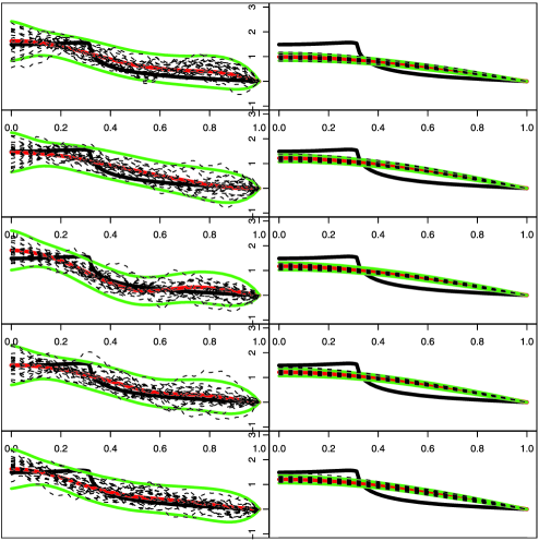
Figure 1: Realizations of the posterior mean (red) and (marginal) posterior credible bands (green), and 20 draws from the posterior (dashed curves). In all ten panels $n=1\mbox{,}000$ and ${\beta}=1$. Left 5 panels: ${\alpha}=1$; right 5 panels: ${\alpha}=5$. True curve (black) given by coefficients ${\mu}_{0,i}=i^{-3/2}\sin(i)$.

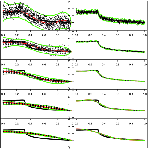
Figure 2: Realizations of the posterior mean (red) and (marginal) posterior credible bands (green), and 20 draws from the posterior (dashed curves). In all ten panels ${\beta}=1$. Left 5 panels: $n=1\mbox{,}000$ and ${\alpha}=0.5,1,2,3,5$ (top to bottom); right 5 panels: $n=10^{8}$ and ${\alpha}=0.5,1,2,3,5$ (top to bottom). True curve (black) given by coefficients ${\mu}_{0,i}=i^{-3/2}\sin(i)$.

Clearly, the posterior mean is not estimating the true curve very well, even for $n=1\mbox{,}000$. This is mostly caused by the intrinsic difficulty of the inverse problem: better estimation requires bigger sample size. A comparison of the left and right panels shows that the rough prior (${\alpha}=1$) is aware of the difficulty: it produces credible bands that in (almost) all cases contain the true curve. On the other hand, the smooth prior (${\alpha}=5$) is overconfident; the spread of the posterior distribution poorly reflects the imprecision of estimation.

Specifying a prior that is too smooth relative to the true curve yields a posterior distribution which gives both a bad reconstruction and a misguided sense of uncertainty. Our theoretical results show that the inaccurate quantification of estimation error remains even as $n\rightarrow\infty$.

The reconstruction, by the posterior mean or any other posterior quantiles, will eventually converge to the true curve. However, specification of a too smooth prior will slow down this convergence significantly. This is illustrated in Figure 2. Every one of its 10 panels is similarly constructed as before, but now with $n=1\mbox{,}000$ and $n=10^{8}$ for the five panels on the left-hand and right-hand side, respectively, and with ${\alpha}=1/2,1,2,3,5$ for the five panels from top to bottom. At first sight ${\alpha}=1$ seems better (see the left column in Figure 2), but leads to zero coverage because of the mismatch close to the bump (see the right column), while ${\alpha}=1/2$ captures the bump. For $n=10^{8}$ the posterior for this optimal prior has collapsed onto the true curve, whereas the smooth posterior for ${\alpha}=5$ still has major difficulty in recovering the bump in the true curve (even though it “thinks” it has captured the correct curve, the bands having collapsed to a single curve in the figure).

7 Proofs

7.1 Proof of Theorem 4.1

The second moment of a Gaussian distribution on $H_{1}$ is equal to the square norm of its mean plus the trace of its covariance operator. Because the posterior is Gaussian $N(AY,S_{n})$, it follows that

$$\int\|{\mu}-{\mu}_{0}\|_{1}^{2}\,d\Pi_{n}({\mu}|Y)=\|AY-{\mu}_{0}\|_{1}^{2}+\operatorname{tr}(S_{n}).$$

By Markov’s inequality, the left-hand side is an upper bound to $M_{n}^{2}{\varepsilon}_{n}^{2}\Pi_{n}({\mu}\dvtx\allowbreak\|{\mu}-{\mu}_{0}\|_{1}\geq M_{n}{\varepsilon}_{n}|Y)$. Therefore, it suffices to show that the expectation under ${\mu}_{0}$ of the right-hand side of the display is bounded by a multiple of ${\varepsilon}_{n}^{2}$. The expectation of the first term is the mean square error of the posterior mean $AY$, and can be written as the sum $\|AK{\mu}_{0}-{\mu}_{0}\|_{1}^{2}+{n}^{-1}\operatorname{tr}(AA^{T})$ of its square bias and “variance.” The second term $\operatorname{tr}(S_{n})$ is deterministic. Under Assumption 3.1 the three quantities can be expressed in the coefficients relative to the eigenbasis $(e_{i})$ as

$$\|AK{\mu}_{0}-{\mu}_{0}\|_{1}^{2} = \sum_{i}\frac{{\mu}_{0,i}^{2}}{(1+n{\lambda}_{i}{\kappa}_{i}^{2})^{2}}\asymp\sum_{i}\frac{\mu_{0,i}^{2}}{(1+n\tau_{n}^{2}i^{-1-2\alpha-2p})^{2}},$$ (14)

$$\frac{1}{n}\operatorname{tr}(AA^{T}) = \sum_{i}\frac{n{\lambda}_{i}^{2}{\kappa}_{i}^{2}}{(1+n{\lambda}_{i}{\kappa}_{i}^{2})^{2}}\asymp\sum_{i}\frac{n\tau_{n}^{4}i^{-2-4\alpha-2p}}{(1+n\tau_{n}^{2}i^{-1-2\alpha-2p})^{2}},$$ (15)

$$\operatorname{tr}(S_{n}) = \sum_{i}\frac{{\lambda}_{i}}{1+n{\lambda}_{i}{\kappa}_{i}^{2}}\asymp\sum_{i}\frac{\tau_{n}^{2}i^{-1-2{\alpha}}}{1+n\tau_{n}^{2}i^{-1-2\alpha-2p}}.$$ (16)

By Lemma 8.1 (applied with $q={\beta}$, $t=0$, $u=1+2{\alpha}+2p$, $v=2$ and $N=n{\tau}_{n}^{2}$), the first can be bounded by $\|{\mu}_{0}\|^{2}_{\beta}(n{\tau}_{n}^{2})^{-({2{\beta}})/({1+2{\alpha}+2p})\wedge 2}$, which accounts for the first term in the definition of ${\varepsilon}_{n}$. By Lemma 8.2 [applied with $\mathcal{S}(i)=1$, $q=-1/2$, $t=2+4{\alpha}+2p$, $u=1+2{\alpha}+2p$, $v=2$, and $N=n{\tau}_{n}^{2}$], and again Lemma 8.2 [applied with $\mathcal{S}(i)=1$, $q=-1/2$, $t=1+2{\alpha}$, $u=1+2{\alpha}+2p$, $v=1$ and $N=n{\tau}_{n}^{2}$], both the second and third expressions are of the order the square of the second term in the definition of ${\varepsilon}_{n}$.

The consequences (i) and (ii) follow by verification after substitution of ${\tau}_{n}$ as given. To prove consequence (iii), we note that the two terms in the definition of ${\varepsilon}_{n}$ are decreasing and increasing in ${\tau}_{n}$, respectively. Therefore, the maximum of these two terms is minimized with respect to ${\tau}_{n}$ by equating the two terms. This minimum (assumed at ${\tau}_{n}=n^{-({1+{\alpha}+2p})/({3+4{\alpha}+6p})}$) is much bigger than $n^{-{\beta}/(1+2{\beta}+2p)}$ if ${\beta}>1+2{\alpha}+2p$.

7.2 Proof of Theorem 5.1

By Proposition 3.2 the posterior distribution is $N(LAY,s_{n}^{2})$, and, hence, similarly as in the proof of Theorem 4.1, it suffices to show that

$$\mathrm{E}_{{\mu}_{0}}|LAY-L{\mu}_{0}|^{2}+s_{n}^{2}=|LAK{\mu}_{0}-L{\mu}_{0}|^{2}+\frac{1}{n}\|LA\|_{1}^{2}+s_{n}^{2}$$

is bounded above by a multiple of $\varepsilon_{n}^{2}$. Under Assumption 3.1 the expressions on the right can be written

$$LAK{\mu}_{0}-L{\mu}_{0} = -\sum_{i}\frac{l_{i}{\mu}_{0,i}}{1+n{\lambda}_{i}{\kappa}_{i}^{2}}\lesssim\sum_{i}\frac{|l_{i}{\mu}_{0,i}|}{1+n{\tau}_{n}^{2}i^{-1-2{\alpha}-2p}},$$ (17)

$$t_{n}^{2}:\! = \frac{1}{n}\|LA\|_{1}^{2}=\sum_{i}\frac{l_{i}^{2}n{\lambda}_{i}^{2}{\kappa}_{i}^{2}}{(1+n{\lambda}_{i}{\kappa}_{i}^{2})^{2}}$$

$$\asymp n{\tau}_{n}^{4}\sum_{i}\frac{l_{i}^{2}i^{-2-4{\alpha}-2p}}{(1+n{\tau}_{n}^{2}i^{-1-2{\alpha}-2p})^{2}},$$

$$s_{n}^{2} = \sum_{i}\frac{l_{i}^{2}{\lambda}_{i}}{1+n{\lambda}_{i}{\kappa}_{i}^{2}}\asymp{\tau}_{n}^{2}\sum_{i}\frac{l_{i}^{2}i^{-1-2{\alpha}}}{1+n{\tau}_{n}^{2}i^{-1-2{\alpha}-2p}}.$$ (19)

By the Cauchy–Schwarz inequality the square of the bias (17) satisfies

$$|LAK{\mu}_{0}-L{\mu}_{0}|^{2}\lesssim\|{\mu}_{0}\|^{2}_{\beta}\sum_{i}\frac{l_{i}^{2}i^{-2{\beta}}}{(1+n{\tau}_{n}^{2}i^{-1-2{\alpha}-2p})^{2}}.$$ (20)

By Lemma 8.1 (applied with $q=q,t=2{\beta},u=1+2{\alpha}+2p,v=2$ and $N=n{\tau}_{n}^{2}$) the right-hand side of this display can be further bounded by $\|{\mu}_{0}\|_{\beta}^{2}\|l\|_{q}^{2}$ times the square of the first term in the sum of two terms that defines ${\varepsilon}_{n}$. By Lemma 8.1 (applied with $q=q,t=2+4{\alpha}+2p,u=1+2{\alpha}+2p,v=2$ and $N=n{\tau}_{n}^{2}$) and again Lemma 8.1 (applied with $q=q,t=1+2{\alpha},u=1+2{\alpha}+2p,v=1$ and $N=n{\tau}_{n}^{2}$), the right-hand sides of (7.2) and (19) are bounded above by $\|l\|^{2}_{q}$ times the square of the second term in the definition of ${\varepsilon}_{n}$.

Consequences (i)–(iv) follow by substitution, and, in the case of (iii), optimization over ${\tau}_{n}$.

7.3 Proof of Theorem 5.2

This follows the same lines as the proof of Theorem 5.1, except that we use Lemma 8.2 (with $q\,{=}\,q,t\,{=}\,2{\beta}$, $u\,{=}\,1\,{+}\,2{\alpha}\,{+}\,2p$, $v\,{=}\,2$ and $N\,{=}\,n{\tau}_{n}^{2}$) and Lemma 8.2 (with $q\,{=}\,q,t\,{=}\,2\,{+}\,4{\alpha}\,{+}\,2p,u\,{=}\,1\,{+}\,2{\alpha}\,{+}\,2p$, $v=2$ and $N=n{\tau}_{n}^{2}$) and again Lemma 8.2 (with $q=q,t=1+2{\alpha},u=1+2{\alpha}+2p$, $v=1$ and $N=n{\tau}_{n}^{2}$) to bound the three terms (7.2)–(20).

7.4 Proof of Theorem 4.2

Because the posterior distribution is $N(AY,\allowbreak S_{n})$, by Proposition 3.1, the radius $r_{n,{\gamma}}$ in (11) satisfies $\mathrm{P}(U_{n}<r_{n,{\gamma}}^{2})=1-{\gamma}$, for $U_{n}$ a random variable distributed as the square norm of an $N(0,S_{n})$-variable. Under (1) the variable $AY$ is $N(AK{\mu}_{0},n^{-1}AA^{T})$-distributed, and, thus, the coverage (12) can be written as

$$\mathrm{P}(\|W_{n}+AK{\mu}_{0}-{\mu}_{0}\|_{1}\leq r_{n,{\gamma}})$$ (21)

for $W_{n}$ possessing a $N(0,n^{-1}AA^{T})$-distribution. For ease of notation let $V_{n}=\|W_{n}\|_{1}^{2}$.

The variables $U_{n}$ and $V_{n}$ can be represented as $U_{n}=\sum_{i}s_{i,n}Z_{i}^{2}$ and $V_{n}=\sum_{i}t_{i,n}Z_{i}^{2}$, for $Z_{1},Z_{2},\ldots$ independent standard normal variables, and $s_{i,n}$ and $t_{i,n}$ the eigenvalues of $S_{n}$ and $n^{-1}AA^{T}$, respectively, which satisfy

$$s_{i,n} = \frac{{\lambda}_{i}}{1+n{\lambda}_{i}{\kappa}_{i}^{2}}\asymp\frac{{\tau}_{n}^{2}i^{-2{\alpha}-1}}{1+n{\tau}_{n}^{2}i^{-2{\alpha}-2p-1}},$$

$$t_{i,n} = \frac{n{\lambda}_{i}^{2}{\kappa}_{i}^{2}}{(1+n{\lambda}_{i}{\kappa}_{i}^{2})^{2}}\asymp\frac{n{\tau}_{n}^{4}i^{-4{\alpha}-2p-2}}{(1+n{\tau}_{n}^{2}i^{-2{\alpha}-2p-1})^{2}},$$

$$s_{i,n}-t_{i,n} = \frac{{\lambda}_{i}}{(1+n{\lambda}_{i}{\kappa}_{i}^{2})^{2}}\asymp\frac{{\tau}_{n}^{2}i^{-2{\alpha}-1}}{(1+n{\tau}_{n}^{2}i^{-2{\alpha}-2p-1})^{2}}.$$

Therefore, by Lemma 8.2 (applied with $\mathcal{S}\equiv 1$ and $q=-1/2$; always the first case),

$$\mathrm{E}U_{n} = \sum_{i}s_{i,n}\asymp{\tau}_{n}^{2}(n{\tau}_{n}^{2})^{-{2{\alpha}}/({1+2{\alpha}+2p})},$$

$$\mathrm{E}V_{n} = \sum_{i}t_{i,n}\asymp{\tau}_{n}^{2}(n{\tau}_{n}^{2})^{-{2{\alpha}}/({1+2{\alpha}+2p})},$$

$$\mathrm{E}(U_{n}-V_{n}) = \sum_{i}(s_{i,n}-t_{i,n})\asymp{\tau}_{n}^{2}(n{\tau}_{n}^{2})^{-{2{\alpha}}/({1+2{\alpha}+2p})},$$

$$\operatorname{var}U_{n} = 2\sum_{i}s_{i,n}^{2}\asymp{\tau}_{n}^{4}(n{\tau}_{n}^{2})^{-({1+4{\alpha}})/({1+2{\alpha}+2p})},$$

$$\operatorname{var}V_{n} = 2\sum_{i}t_{i,n}^{2}\asymp{\tau}_{n}^{4}(n{\tau}_{n}^{2})^{-({1+4{\alpha}})/({1+2{\alpha}+2p})}.$$

We conclude that the standard deviations of $U_{n}$ and $V_{n}$ are negligible relative to their means, and also relative to the difference $\mathrm{E}(U_{n}-V_{n})$ of their means. Because $U_{n}\geq V_{n}$, we conclude that the distributions of $U_{n}$ and $V_{n}$ are asymptotically completely separated: $\mathrm{P}(V_{n}\leq v_{n}\leq U_{n})\to 1$ for some $v_{n}$ [e.g., $v_{n}=\mathrm{E}(U_{n}+V_{n})/2$]. The numbers $r_{n,{\gamma}}^{2}$ are $1-{\gamma}$-quantiles of $U_{n}$, and, hence, $\mathrm{P}(V_{n}\leq r^{2}_{n,{\gamma}}(1+o(1)))\rightarrow 1$. Furthermore, it follows that

$$r_{n,{\gamma}}^{2}\asymp{\tau}_{n}^{2}(n{\tau}_{n}^{2})^{-{2{\alpha}}/({1+2{\alpha}+2p})}\asymp\mathrm{E}U_{n}\asymp\mathrm{E}V_{n}.$$

The square norm of the bias $AK{\mu}_{0}-{\mu}_{0}$ is given in (14), where it was noted that

$$B_{n}:={\sup_{\|{\mu}_{0}\|_{\beta}\lesssim 1}}\|AK{\mu}_{0}-{\mu}_{0}\|_{1}\asymp(n{\tau}_{n}^{2})^{-{\beta}/({1+2{\alpha}+2p})\wedge 1}.$$

The bias $B_{n}$ is decreasing in ${\tau}_{n}$, whereas $\mathrm{E}U_{n}$ and $\operatorname{var}U_{n}$ are increasing. The scaling rate $\tilde{\tau}_{n}\asymp n^{({\alpha}-\tilde{\beta})/(1+2\tilde{\beta}+2p)}$ balances the square bias $B_{n}^{2}$ with the variance $\mathrm{E}V_{n}$ of the posterior mean, and hence with $r_{n,{\gamma}}^{2}$.

Case (i). In this case $B_{n}\ll r_{n,{\gamma}}$. Hence, $\mathrm{P}(\|W_{n}+AK{\mu}_{0}-{\mu}_{0}\|_{1}\leq r_{n,{\gamma}})\geq\mathrm{P}(\|W_{n}\|_{1}\leq r_{n,{\gamma}}-B_{n})=\mathrm{P}(V_{n}\leq r_{n,{\gamma}}^{2}(1+o(1)))\rightarrow 1$, uniformly in the set of ${\mu}_{0}$ in the supremum defining $B_{n}$.

Case (iii). In this case $B_{n}\gg r_{n,{\gamma}}$. Hence, $\mathrm{P}(\|W_{n}+AK{\mu}_{0}^{n}-{\mu}_{0}^{n}\|_{1}\leq r_{n,{\gamma}})\leq\mathrm{P}(\|W_{n}\|_{1}\geq B_{n}-r_{n,{\gamma}})\rightarrow 0$ for any sequence ${\mu}_{0}^{n}$ (nearly) attaining the supremum in the definition of $B_{n}$. If ${\tau}_{n}\equiv 1$, then $B_{n}$ and $r_{n,{\gamma}}$ are both powers of $1/n$ and, hence, $B_{n}\gg r_{n,{\gamma}}$ implies that $B_{n}\gtrsim r_{n,{\gamma}}n^{\delta}$, for some ${\delta}>0$. The preceding argument then applies for a fixed ${\mu}_{0}$ of the form ${\mu}_{0,i}\asymp i^{-1/2-{\beta}-{\varepsilon}}$, for small ${\varepsilon}>0$, that gives a bias that is much closer than $n^{\delta}$ to $B_{n}$.

Case (ii). In this case $B_{n}\asymp r_{n,{\gamma}}$. If ${\beta}<1+2{\alpha}+2p$, then by the second assertion (first case) of Lemma 8.1 the bias $\|AK{\mu}_{0}-{\mu}_{0}\|_{1}$ at a fixed ${\mu}_{0}$ is of strictly smaller order than the supremum $B_{n}$. The argument of (i) shows that the asymptotic coverage then tends to 1.

Finally, we prove the existence of a sequence ${\mu}_{0}^{n}$ along which the coverage is a given $c\in[0,1)$. The coverage (21) with ${\mu}_{0}$ replaced by ${\mu}_{0}^{n}$ tends to $c$ if, for $b_{n}=AK{\mu}_{0}^{n}-{\mu}_{0}^{n}$ and $z_{c}$ a standard normal quantile,

$$\frac{\|W_{n}+b_{n}\|_{1}^{2}-\mathrm{E}\|W_{n}+b_{n}\|_{1}^{2}}{{\operatorname{sd}}\|W_{n}+b_{n}\|_{1}^{2}} \rightsquigarrow N(0,1),$$ (22)

$$\frac{r_{n,{\gamma}}^{2}-\mathrm{E}\|W_{n}+b_{n}\|_{1}^{2}}{{\operatorname{sd}}\|W_{n}+b_{n}\|_{1}^{2}} \rightarrow z_{c}.$$ (23)

Because $W_{n}$ is mean-zero Gaussian, we have $\mathrm{E}\|W_{n}+b_{n}\|_{1}^{2}=\mathrm{E}\|W_{n}\|_{1}^{2}+\|b_{n}\|_{1}^{2}$ and ${\operatorname{var}}\|W_{n}+b_{n}\|_{1}^{2}={\operatorname{var}}\|W_{n}\|_{1}^{2}+4\operatorname{var}\langle W_{n},b_{n}\rangle_{1}$. Here $\|W_{n}\|_{1}^{2}=V_{n}$ and the distribution of $\langle W_{n},b_{n}\rangle_{1}$ is zero-mean Gaussian with variance $\langle b_{n},n^{-1}AA^{T}b_{n}\rangle_{1}$. With $t_{i,n}$ the eigenvalues of $n^{-1}AA^{T}$, display (23) can be translated in the coefficients $(b_{n,i})$ of $b_{n}$ relative to the eigenbasis, as

$$\frac{r_{n,{\gamma}}^{2}-\mathrm{E}V_{n}-\sum_{i}b_{n,i}^{2}}{\sqrt{\operatorname{var}V_{n}+4\sum_{i}t_{i,n}b_{n,i}^{2}}}\rightarrow z_{c}.$$ (24)

We choose $(b_{n,i})$ differently in the cases that ${\beta}\leq 1+2{\alpha}+2p$ and ${\beta}\geq 1+2{\alpha}+2p$, respectively. In both cases the sequence has exactly one nonzero coordinate. We denote this coordinate by $b_{n,i_{n}}$, and set, for numbers $d_{n}$ to be determined,

$$b_{n,i_{n}}^{2}=r_{n,{\gamma}}^{2}-\mathrm{E}V_{n}-d_{n}\operatorname{sd}V_{n}.$$

Because $r_{n,{\gamma}}^{2}$, $\mathrm{E}V_{n}$ and $r_{n,{\gamma}}^{2}-\mathrm{E}V_{n}$ are of the same order of magnitude, and $\operatorname{sd}V_{n}$ is of strictly smaller order, for bounded or slowly diverging $d_{n}$ the right-hand side of the preceding display is equivalent to $(r_{n,{\gamma}}^{2}-\mathrm{E}V_{n})(1+o(1))$. Consequently, the left-hand side of (24) is equivalent to

$$\frac{d_{n}\operatorname{sd}V_{n}}{\sqrt{\operatorname{var}V_{n}+4t_{i_{n},n}(r_{n,{\gamma}}^{2}-\mathrm{E}V_{n})(1+o(1))}}.$$

The remainder of the argument is different in the two cases.

Case ${\beta}\leq 1+2{\alpha}+2p$. We choose $i_{n}\asymp(n{\tau}_{n}^{2})^{1/(1+2{\alpha}+2p)}$. It can be verified that $t_{i_{n},n}(r_{n,{\gamma}}^{2}-\mathrm{E}V_{n})/\operatorname{var}V_{n}\asymp 1$. Therefore, for $c\in[0,1]$, there exists a bounded or slowly diverging sequence $d_{n}$ such that the preceding display tends to $z_{c}$.

The bias $b_{n}$ results from a parameter ${\mu}_{0}^{n}$ such that $b_{n,i}=(1+n{\lambda}_{i}{\kappa}_{i}^{2})^{-1}({\mu}_{0}^{n})_{i}$, for every $i$. Thus, ${\mu}_{0}^{n}$ also has exactly one nonzero coordinate, and this is proportional to the corresponding coordinate of $b_{n}$, by the definition of $i_{n}$. It follows that

$$i_{n}^{2{\beta}}({\mu}_{0}^{n})^{2}_{i_{n}}\asymp i_{n}^{2{\beta}}b_{n,i_{n}}^{2}\lesssim i_{n}^{2{\beta}}(r_{n,{\gamma}}^{2}-\mathrm{E}V_{n})\asymp 1$$

by the definition of ${\tau}_{n}$. It follows that $\|{\mu}_{0}^{n}\|_{\beta}\lesssim 1$.

Case ${\beta}\geq 1+2{\alpha}+2p$. We choose $i_{n}=1$. In this case ${\tau}_{n}\rightarrow 0$ and it can be verified that $t_{i_{n},n}(r_{n,{\gamma}}^{2}-\mathrm{E}V_{n})/\operatorname{var}V_{n}\rightarrow 0$. Also,

$$({\mu}_{0}^{n})_{1}^{2}\asymp(1+n{\tau}_{n}^{2})^{2}b_{n,1}^{2}\lesssim(1+n{\tau}_{n}^{2})^{2}\mathrm{E}V_{n}.$$

This is $O(1)$, because ${\tau}_{n}$ is chosen so that $\mathrm{E}V_{n}$ is of the same order as the square bias $B_{n}^{2}$, which is $(n{\tau}_{n}^{2})^{-2}$ in this case.

It remains to prove the asymptotic normality (22). We can write

$$\|W_{n}+b_{n}\|_{1}^{2}-\mathrm{E}\|W_{n}+b_{n}\|_{1}^{2}=\sum_{i}t_{i,n}(Z_{i}^{2}-1)+2b_{n,i_{n}}\sqrt{t_{{i_{n}},n}}Z_{i_{n}}.$$

The second term is normal by construction. The first term has variance $2\sum_{i}t_{i,n}^{2}$. With some effort it can be seen that

$$\sup_{i}\frac{t_{i,n}^{2}}{\sum_{i}t_{i,n}^{2}}\rightarrow 0.$$

Therefore, by a slight adaptation of the Lindeberg–Feller theorem (to infinite sums), we have that $\sum_{i}t_{i,n}(Z_{i}^{2}-1)$ divided by its standard deviation tends in distribution to the standard normal distribution. Furthermore, the preceding display shows that this conclusion does not change if the $i_{n}$th term is left out from the infinite sum. Thus, the two terms converge jointly to asymptotically independent standard normal variables, if scaled separately by their standard deviations. Then their scaled sum is also asymptotically standard normally distributed.

7.5 Proof of Theorem 5.3

Under (1) the variable $LAY$ is $N(LAK{\mu}_{0},\allowbreak t_{n}^{2})$-distributed, for $t_{n}^{2}$ given in (7.2). It follows that the coverage can be written, with $W$ a standard normal variable,

$$\mathrm{P}(|Wt_{n}+LAK{\mu}_{0}-L{\mu}_{0}|\leq-s_{n}z_{{\gamma}/2}).$$ (25)

The bias $LAK{\mu}_{0}-L{\mu}_{0}$ and posterior spread $s_{n}^{2}$ are expressed as a series in (17) and (19).

In the proof of Theorem 5.2 $s_{n}$ and $t_{n}$ were seen to have the same order of magnitude, given by the second term in ${\varepsilon}_{n}$ given in (13), with a slowly varying term ${\delta}_{n}$ as given in the theorem,

$$s_{n}\asymp t_{n}\asymp{\tau}_{n}(n{\tau}_{n}^{2})^{-(1/2+{\alpha}+q)/(1+2{\alpha}+2p)}{\delta}_{n}.$$ (26)

Furthermore, $t_{n}\leq s_{n}$ for every $n$, as every term in the infinite series (7.2) is $n{\lambda}_{i}{\kappa}_{i}^{2}/(1+n{\lambda}_{i}{\kappa}_{i}^{2})\leq 1$ times the corresponding term in (19).

Because $W$ is centered, the coverage (25) is largest if the bias $LAK{\mu}_{0}-L{\mu}_{0}$ is zero. It is then at least $1-{\gamma}$, because $t_{n}\leq s_{n}$; remains strictly smaller than $1$, because $t_{n}\asymp s_{n}$; and tends to exactly $1-{\gamma}$ iff $s_{n}/t_{n}\rightarrow 1$. By Theorem 5.4(i) the latter is impossible if $q<p$. The analysis for nonzero ${\mu}_{0}$ depends strongly on the size of the bias relative to $t_{n}$.

The supremum of the bias satisfies, for ${\gamma}_{n}$ the slowly varying term given in Theorem 5.2,

$$B_{n}:={\sup_{\|{\mu}_{0}\|_{\beta}\lesssim 1}}|LAK{\mu}_{0}-L{\mu}_{0}|\asymp(n{\tau}_{n}^{2})^{-(({\beta}+q)/(1+2{\alpha}+2p))\wedge 1}{\gamma}_{n}.$$ (27)

That the left-hand side of (27) is smaller than the right-hand side was already shown in the proof of Theorem 5.2, with the help of Lemma 8.2. That this upper bound is sharp follows by considering the sequence ${\mu}_{0}^{n}$ defined by, with $\tilde{B}_{n}$ the right-hand side of the preceding display,

$${\mu}_{0,i}^{n}=\frac{1}{\tilde{B}_{n}}\frac{i^{-2{\beta}}l_{i}}{1+n{\tau}_{n}^{2}i^{-1-2{\alpha}-2p}}.$$

[This is the sequence that gives equality in the application of the Cauchy–Schwarz inequality to derive (20).] Using Lemma 8.2, it can be seen that $\|{\mu}_{0}^{n}\|_{\beta}\lesssim 1$ and that the bias at ${\mu}_{0}^{n}$ is of the order $\tilde{B}_{n}$.

By Lemma 8.3, the bias at a fixed ${\mu}_{0}\in S^{\beta}$ is of strictly smaller order than the supremum $B_{n}$ if ${\beta}+q<1+2{\alpha}+2p$.

The maximal bias $B_{n}$ is a decreasing function of the scaling parameter ${\tau}_{n}$, while the standard deviation $t_{n}$ and root-spread $s_{n}$ increase with ${\tau}_{n}$. The scaling rate $\tilde{\tau}_{n}$ in the statement of the theorem balances $B_{n}$ with $s_{n}\asymp t_{n}$.

Case (i). If ${\tau}_{n}\gg\tilde{\tau}_{n}$, then $B_{n}\ll t_{n}$. Hence, the bias $LAK{\mu}_{0}-L{\mu}_{0}$ in (25) is negligible relative to $t_{n}\asymp s_{n}$, uniformly in $\|{\mu}_{0}\|_{\beta}\lesssim 1$, and the coverage is asymptotic to $\mathrm{P}(|Wt_{n}|\leq-s_{n}z_{{\gamma}/2})$, which is asymptotically strictly between $1-{\gamma}$ and $1$.

Case (iii). If ${\tau}_{n}\ll\tilde{\tau}_{n}$, then $B_{n}\gg t_{n}$. If $b_{n}=LAK{\mu}_{0}^{n}-L{\mu}_{0}^{n}$ is the bias at a sequence ${\mu}_{0}^{n}$ that (nearly) attains the supremum in the definition of $B_{n}$, then the coverage at ${\mu}_{0}^{n}$ satisfies $\mathrm{P}(|Wt_{n}+b_{n}|\leq-s_{n}z_{{\gamma}/2})\leq\mathrm{P}(|Wt_{n}|\geq b_{n}-s_{n}|z_{{\gamma}/2}|)\rightarrow 0$, as $b_{n}\asymp B_{n}\gg s_{n}$. By the same argument, the coverage also tends to zero for a fixed ${\mu}_{0}$ in $S^{\beta}$ with bias $b_{n}=LAK{\mu}_{0}-L{\mu}_{0}\gg t_{n}$. For this we choose ${\mu}_{0,i}=i^{-{\beta}}i^{q}l_{i}\tilde{S}(i)$ for a slowly varying function such that $\sum_{i}\mathcal{S}^{2}(i)\tilde{S}^{2}(i)/i<\infty$. The latter condition ensures that $\|{\mu}_{0}\|_{\beta}<\infty$. By another application of Lemma 8.2, the bias at ${\mu}_{0}$ is of the order [cf. (17)]

$$\sum_{i}\frac{l_{i}{\mu}_{0,i}}{1+n{\tau}_{n}^{2}i^{-1-2{\alpha}-2p}}=\sum_{i}\frac{(l_{i}\tilde{S}^{1/2}(i))^{2}i^{-{\beta}+q}}{1+n{\tau}_{n}^{2}i^{-1-2{\alpha}-2p}}\asymp(n{\tau}_{n}^{2})^{-({{\beta}+q})/({1+2{\alpha}+2p})\wedge 1}\tilde{\gamma}_{n},$$

where, for ${\rho}_{n}=(n{\tau}_{n}^{2})^{1/(1+2{\alpha}+2p)}$,

$$\tilde{\gamma}_{n}^{2}=\cases{\mathcal{S}^{2}({\rho}_{n})\tilde{S}({\rho}_{n}),&\quad if ${\beta}+q<1+2{\alpha}+2p$,\vspace*{2pt}\cr\displaystyle\sum_{i\leq{\rho}_{n}}\frac{\mathcal{S}^{2}(i)\tilde{S}(i)}{i},&\quad if ${\beta}+q=1+2{\alpha}+2p$,\vspace*{2pt}\cr 1,&\quad if ${\beta}+q>1+2{\alpha}+2p$.}$$

Therefore, the bias at ${\mu}_{0}$ has the same form as the maximal bias $B_{n}$; the difference is in the slowly varying factor $\tilde{\gamma}_{n}$. If ${\tau}_{n}\leq\tilde{\tau}_{n}n^{-{\delta}}$, then $B_{n}\gtrsim t_{n}n^{{\delta}^{\prime}}$ for some ${\delta}^{\prime}>0$ and, hence, $b_{n}\asymp B_{n}\tilde{\gamma}_{n}/{\gamma}_{n}\gg t_{n}$.

Case (ii). If ${\tau}_{n}\asymp\tilde{\tau}_{n}$, then $B_{n}\asymp t_{n}$. If $b_{n}=LAK{\mu}_{0}^{n}-L{\mu}_{0}^{n}$ is again the bias at a sequence ${\mu}_{0}^{n}$ that nearly assumes the supremum in the definition of $B_{n}$, we have that $\mathrm{P}(|Wt_{n}+db_{n}|\leq-s_{n}z_{{\gamma}/2})\leq\mathrm{P}(|Wt_{n}|\geq db_{n}-s_{n}|z_{{\gamma}/2}|)$ attains an arbitrarily small value if $d$ is chosen sufficiently large. This is the coverage at the sequence $d{\mu}_{0}^{n}$, which is bounded in $S^{\beta}$. On the other hand, the bias at a fixed ${\mu}_{0}\in S^{\beta}$ is of strictly smaller order than the supremum $B_{n}$, and, hence, the coverage at a fixed ${\mu}_{0}$ is as in case (i).

If the scaling rate is fixed to ${\tau}_{n}\equiv 1$, then it can be checked from (26) and (27) that $B_{n}\ll t_{n}$, $B_{n}\asymp t_{n}$ and $B_{n}\gg t_{n}$ in the three cases ${\alpha}<{\beta}-1/2$, ${\alpha}={\beta}-1/2$ and ${\alpha}>{\beta}-1/2$, respectively. In the first and third cases the maximal bias and the spread differ by more than a polynomial term $n^{\delta}$; in the second case it must be noted that the slowly varying terms ${\gamma}_{n}$ and ${\delta}_{n}$ are equal [to $\mathcal{S}({\rho}_{n})$]. It follows that the preceding analysis (i), (ii), (iii) extends to this situation.

7.6 Proof of Theorem 5.4

(i). The two quantities $s_{n}$ and $t_{n}$ are given as series in (19) and (7.2). Every term in the series (7.2) is $n{\lambda}_{i}{\kappa}_{i}^{2}/(1+n{\lambda}_{i}{\kappa}_{i}^{2})\leq 1$ times the corresponding term in the series (19). Therefore, $s_{n}/t_{n}\rightarrow 1$ if and only if the series are determined by the terms for which these numbers are “close to” 1, that is, $n{\lambda}_{i}{\kappa}_{i}^{2}$ is large. More precisely, we show below that $s_{n}/t_{n}\rightarrow 1$ if and only if, for every $c>0$,

$$\sum_{n{\lambda}_{i}{\kappa}_{i}^{2}\leq c}\frac{l_{i}^{2}{\lambda}_{i}}{1+n{\lambda}_{i}{\kappa}_{i}^{2}}=o\biggl{(}\sum_{i}\frac{l_{i}^{2}{\lambda}_{i}}{1+n{\lambda}_{i}{\kappa}_{i}^{2}}\biggr{)}.$$ (28)

If $l\in S^{p}$, then the series on the left is as in Lemma 8.1 with $q=p$, $u=1+2{\alpha}+2p$, $v=1$, $N=n{\tau}_{n}^{2}$ and $t=1+2{\alpha}$. Hence, $(t+2q)/u\geq v$, and the display follows from the final assertion of the lemma. If $l_{i}=i^{-q-1/2}\mathcal{S}(i)$ for a slowly varying function $\mathcal{S}$, then the series is as in Lemma 8.2, with the same parameters, and by the last statement of the lemma the display is true if and only if $(t+2q)/u\geq v$, that is, $q\geq p$.

To prove that (28) holds iff $s_{n}/t_{n}\rightarrow 1$, write $s_{n}^{2}=A_{n}+B_{n}$, for $A_{n}$ and $B_{n}$ the sums over the terms in (19) with $n{\lambda}_{i}{\kappa}_{i}^{2}>c$ and $n{\lambda}_{i}{\kappa}_{i}^{2}\leq c$, respectively, and, similarly, $t_{n}^{2}=C_{n}+D_{n}$. Then

$$\frac{D_{n}}{B_{n}}\leq\frac{c}{1+c}\leq\frac{C_{n}}{A_{n}}\leq 1.$$

It follows that

$$\frac{t_{n}^{2}}{s_{n}^{2}}=\frac{C_{n}+D_{n}}{A_{n}+B_{n}}=\frac{C_{n}/A_{n}+(D_{n}/B_{n})(B_{n}/A_{n})}{1+B_{n}/A_{n}}\leq\frac{1+c/(1+c)(B_{n}/A_{n})}{1+B_{n}/A_{n}}.$$

Because $x\mapsto(1+rx)/(1+x)$ is strictly decreasing from 1 at $x=0$ to $r<1$ at $x=\infty$ (if $0<r<1$), the right-hand side of the equation is asymptotically 1 if and only if $B_{n}/A_{n}\to 0$, and otherwise its liminf is strictly smaller. Thus, $t_{n}/s_{n}\to 1$ implies that $B_{n}/A_{n}\to 0$. Second,

$$\frac{t_{n}^{2}}{s_{n}^{2}}\geq\frac{C_{n}}{A_{n}+B_{n}}=\frac{C_{n}/A_{n}}{1+B_{n}/A_{n}}\geq\frac{c/(1+c)}{1+B_{n}/A_{n}}.$$

It follows that $\liminf t_{n}^{2}/s_{n}^{2}\geq c/(1+c)$ if $B_{n}/A_{n}\to 0$. This being true for every $c>0$ implies that $t_{n}/s_{n}\to 1$.

i(i) Second assertion. If $l\in S^{p}$, then we apply Lemma 8.1 with $q=p$, $t=1+2{\alpha}$, $u=1+2{\alpha}+2p$, $v=1$ and $N=n{\tau}_{n}^{2}$ to see that $s_{n}^{2}\asymp{\tau}_{n}^{2}(n{\tau}_{n}^{2})^{-v}=n^{-1}$. Furthermore, the second assertion of the lemma with $(uv-t)/2=p$ shows that $ns_{n}^{2}\rightarrow\|l\|_{p}^{2}=\sum_{i}l_{i}^{2}/{\kappa}_{i}^{2}$ in the case that ${\kappa}_{i}=i^{-p}$. The proof can be extended to cover the slightly more general sequence $({\kappa}_{i})$ in Assumption 3.1.

If $l\in\mathcal{R}^{q}$, then we apply Lemma 8.2 with $q=p$, $t=1+2{\alpha}$, $u=1+2{\alpha}+2p$, $v=1$ and $N=n{\tau}_{n}^{2}$ to see that $s_{n}^{2}\asymp n^{-1}\sum_{i\leq N^{1/u}}\mathcal{S}^{2}(i)/i$.

(ii) If $l\in S^{q}$, then the bias is bounded above in (20), and in the proof of Theorem 5.1 its supremum $B_{n}$ over $\|{\mu}_{0}\|_{\beta}\lesssim 1$ is seen to be bounded by $(n{\tau}_{n}^{2})^{-({\beta}+q)/(1+2{\alpha}+2p)\wedge 1}$, the first term in the definition of ${\varepsilon}_{n}$ in the statement of this theorem. This upper bound is $o(n^{-1/2})$ iff the stated conditions hold. [Here we use that $\mathcal{S}^{2}(N)\ll\sum_{i\leq N}\mathcal{S}^{2}(i)/i$ as $N\rightarrow\infty$, as noted in the proof of Lemma 8.2.]

The supremum of the bias $B_{n}$ in the case that $l\in\mathcal{R}^{q}$ is given in (27). It was already seen to be $o(t_{n})$ if ${\tau}\gg\tilde{\tau}_{n}$ in the proof of case (i) of Theorem 5.3. If ${\tau}_{n}=1$, we have that $B_{n}\asymp n^{-({\beta}+q)/(1+2{\alpha}+2p)\wedge 1}{\gamma}_{n}$, for ${\gamma}_{n}$ the slowly varying factor given in the statement of Theorem 5.2. Furthermore, we have $s_{n}\asymp t_{n}\asymp n^{-1/2}{\delta}_{n}$, for ${\delta}_{n}$ the slowly varying factor in the same statement. Under the present conditions, ${\delta}_{n}\asymp 1$ if $q>p$ and ${\delta}_{n}^{2}\asymp\sum_{i\leq{\rho}_{n}}\mathcal{S}^{2}(i)/i$ if $q=p$. We can now verify that $B_{n}=o(t_{n})$ if and only if the conditions as stated hold.

(iii) The total variation distance between two Gaussian distributions with the same expectation and standard deviations $s_{n}$ and $t_{n}$ tends to zero if and only if $s_{n}/t_{n}\rightarrow 1$. Similarly, the total distance between two Gaussians with the same standard deviation $s_{n}$ and means ${\mu}_{n}$ and ${\nu}_{n}$ tends to zero if and only if ${\mu}_{n}-{\nu}_{n}=o(s_{n})$. Therefore, it suffices to show that $(LAY-\sum_{i}Y_{i}l_{i}/{\kappa}_{i})/s_{n}\rightarrow 0$ if $l\in S^{p}$. Because the bias was already seen to be $o(t_{n})$ and $s_{n}\asymp n^{-1/2}$ if $l\in S^{p}$, it suffices to show that $LAZ-\sum_{i}Z_{i}l_{i}/{\kappa}_{i}\rightarrow 0$. Under Assumption 3.1 this difference is equal to

$$\sum_{i}\frac{{\kappa}_{i}{\lambda}_{i}l_{i}Z_{i}}{n^{-1}+{\kappa}_{i}^{2}{\lambda}_{i}}-\sum_{i}Z_{i}\frac{l_{i}}{{\kappa}_{i}}=\sum_{i}\frac{Z_{i}l_{i}}{{\kappa}_{i}}\biggl{(}\frac{1}{1+n{\kappa}_{i}^{2}{\lambda}_{i}}\biggr{)}.$$

If $\sum_{i}l_{i}^{2}/{\kappa}_{i}^{2}<\infty$, then the variance of this expression is seen to tend to zero by dominated convergence.

The final assertion of the theorem follows along the lines of the proof of Theorem 5.3.

8 Technical lemmas

Lemma 8.1

For any $q\geq 0$, $t\geq-2q$, $u>0$ and $v\geq 0$, as $N\to\infty$,

$$\sup_{\|\xi\|_{q}\leq 1}\sum_{i}\frac{\xi_{i}^{2}i^{-t}}{(1+Ni^{-u})^{v}}\asymp N^{-((t+2q)/u)\wedge v}.$$

Moreover, for every fixed $\xi\in S^{q}$, as $N\to\infty$,

$$N^{((t+2q)/u)\wedge v}\sum_{i}\frac{\xi_{i}^{2}i^{-t}}{(1+Ni^{-u})^{v}}\rightarrow\cases{0,&\quad if $(t+2q)/u<v$,\cr\|\xi\|^{2}_{(uv-t)/{2}},&\quad if $(t+2q)/u\geq v$.}$$

The last assertion remains true if the sum is limited to the terms $i\leq cN^{1/u}$, for any $c>0$.

In the range $i\leq N^{1/u}$ we have $Ni^{-u}\leq 1+Ni^{-u}\leq 2Ni^{-u}$, while $1\leq 1+Ni^{-u}\leq 2$ in the range $i>N^{1/u}$. Thus, deleting either the first or second term, we obtain

$$\sum_{i\leq N^{1/u}}\frac{\xi_{i}^{2}i^{-t}}{(1+Ni^{-u})^{v}} \asymp \sum_{i\leq N^{1/u}}\xi_{i}^{2}i^{2q}\frac{i^{uv-t-2q}}{N^{v}}\leq\|\xi\|_{q}^{2}N^{-((t+2q)/u)\wedge v},$$

$$\sum_{i>N^{1/u}}\frac{\xi_{i}^{2}i^{-t}}{(1+Ni^{-u})^{v}} \asymp \sum_{i>N^{1/u}}\xi_{i}^{2}i^{2q}i^{-t-2q}\leq N^{-(t+2q)/u}\sum_{i>N^{1/u}}\xi_{i}^{2}i^{2q}.$$

The inequality in the first line follows by bounding $i$ in $i^{uv-t-2q}$ by $N^{1/u}$ if $uv-t-2q>0$, and by 1 otherwise. This proves the upper bound for the supremum.

The lower bound follows by considering the two sequences $(\xi_{i})$ given by $\xi_{i}=i^{-q}$ for $i\sim N^{1/u}$ and $\xi_{i}=0$ otherwise (showing that the supremum is bigger than $N^{-(t+2q)/u}$), and given by $\xi_{1}=1$ and $\xi_{i}=0$ otherwise (showing that the supremum is bigger than $N^{-v}$).

The second line of the preceding display shows that the sum over the terms $i>N^{1/u}$ is $o(N^{-(t+2q)/u})$. Furthermore, the first line can be multiplied by $N^{(t+2q)/u}$ to obtain

$$N^{(t+2q)/u}\sum_{i\leq N^{1/u}}\frac{\xi_{i}^{2}i^{-t}}{(1+Ni^{-u})^{v}}\asymp\sum_{i\leq N^{1/u}}\xi_{i}^{2}i^{2q}\biggl{(}\frac{i}{N^{1/u}}\biggr{)}^{uv-t-2q}.$$

If $(t+2q)/u<v$, then $uv-t-2q>0$ and this tends to zero by dominated convergence. Also,

$$N^{v}\sum_{i}\frac{\xi_{i}^{2}i^{-t}}{(1+Ni^{-u})^{v}}=\sum_{i}\xi_{i}^{2}i^{uv-t}\biggl{(}\frac{Ni^{-u}}{1+Ni^{-u}}\biggr{)}^{v}.$$

If $(t+2q)/u\geq v$, then $q\geq(uv-t)/2$ and, hence, $\xi\in S^{{(uv-t)}/{2}}$, and the right-hand side tends to $\sum_{i}\xi_{i}^{2}i^{uv-t}$ by dominated convergence.

The final assertion needs to be proved only in the case that $(t+2q)/u\geq v$, as in the other case the whole sum tends to 0. The sum over the terms $i>N^{1/u}$ was seen to be always $o(N^{-(t+2q)/u})$, which is $o(N^{-v})$ if $(t+2q)/u\geq v$. The final assertion for $c=1$ follows, because the sum over the terms $i\leq N^{1/u}$ was seen to have the exact order $N^{-v}$ (if $\xi\not=0$). For general $c$ the proof is analogous, or follows by scaling $N$.

Lemma 8.2

For any $t,v\geq 0$, $u>0$, and $(\xi_{i})$ such that $|\xi_{i}|=i^{-q-1/2}\mathcal{S}(i)$ for $q>-t/2$ and a slowly varying function $\mathcal{S}\dvtx(0,\infty)\to(0,\infty)$, as $N\rightarrow\infty$,

$$\sum_{i}\frac{\xi_{i}^{2}i^{-t}}{(1+Ni^{-u})^{v}}\asymp\cases{N^{-(t+2q)/u}\mathcal{S}^{2}(N^{1/u}),&\quad if $(t+2q)/u<v$,\vspace*{2pt}\cr\displaystyle N^{-v}\sum_{i\leq N^{1/u}}\mathcal{S}^{2}(i)\big{/}i,&\quad if $(t+2q)/u=v$,\vspace*{2pt}\cr N^{-v},&\quad if $(t+2q)/u>v$.}$$

Moreover, for every $c>0$, the sum on the left is asymptotically equivalent to the same sum restricted to the terms $i\leq cN^{1/u}$ if and only if $(t+2q)/u\geq v$.

As in the proof of the preceding lemma, we split the infinite series in the sum over the terms $i\leq N^{1/u}$ and $i>N^{1/u}$. For the first part of the series

$$\sum_{i\leq N^{1/u}}\frac{\xi_{i}^{2}i^{-t}}{(1+Ni^{-u})^{v}}\asymp\sum_{i\leq N^{1/u}}\mathcal{S}(i)^{2}\frac{i^{uv-t-2q-1}}{N^{v}}.$$

If $uv-t-2q>0$ [i.e., $(t+2q)/u<v$], the right-hand side is of the order $N^{-(t+2q)/u}\mathcal{S}^{2}(N^{1/u})$, by Theorem 1(b) on page 281 in Feller , while if $uv-t-2q<0$, it is of the order $N^{-v}$ by Lemma on page 280 in Feller . Finally, if $uv-t-2q=0$, then the right-hand side is identical to $N^{-v}\sum_{i\leq N^{1/u}}{\mathcal{S}^{2}(i)}/{i}$.

The other part of the infinite series satisfies, by Theorem 1(a) on page 281 in Feller ,

$$\sum_{i>N^{1/u}}\frac{\xi_{i}^{2}i^{-t}}{(1+Ni^{-u})^{v}}\asymp\sum_{i>N^{1/u}}\mathcal{S}(i)^{2}i^{-t-2q-1}\asymp N^{-(t+2q)/u}\mathcal{S}^{2}(N^{1/u}).$$

This is never bigger than the contribution of the first part of the sum, and of equal order if $(t+2q)/u<v$. If $(t+2q)/u>v$, then the leading polynomial term is strictly smaller than $N^{-v}$. If $(t+2q)/u=v$, then the leading term is equal to $N^{-v}$, but the slowly varying part satisfies $\mathcal{S}^{2}(N^{1/u})\ll\sum_{i\leq N^{1/u}}{\mathcal{S}^{2}(i)}/{i}$, by Theorem 1(b) on page 281 in Feller . Therefore, in both cases the preceding display is negligible relative to the first part of the sum. This proves the final assertion of the lemma for $c=1$. The proof for general $c>0$ is analogous.

By the Cauchy–Schwarz inequality, for any ${\mu}\in S^{t/2}$,

$$\biggl{|}\sum_{i}\frac{\xi_{i}\mu_{i}}{1+Ni^{-u}}\biggr{|}^{2}\leq\|{\mu}\|_{t/2}^{2}\sum_{i}\frac{\xi_{i}^{2}i^{-t}}{(1+Ni^{-u})^{2}}.$$

The preceding lemma gives the exact order of the right-hand side. The application of the Cauchy–Schwarz inequality is sharp, in that there is equality for some $\mu\in S^{t/2}$. However, this $\mu$ depends on $N$. For fixed $\mu\in S^{t/2}$ the left-hand side is strictly smaller than the right-hand side.

Lemma 8.3

For any $t,u\geq 0$, $\mu\in S^{t/2}$ and $(\xi_{i})$ such that $|\xi_{i}|=\break i^{-q-1/2}\mathcal{S}(i)$ for $0<t+2q<2u$ and a slowly varying function $\mathcal{S}\dvtx(0,\infty)\to(0,\infty)$, as $N\rightarrow\infty$,

$$\sum_{i}\frac{|\xi_{i}\mu_{i}|}{1+Ni^{-u}}\ll N^{-(t+2q)/(2u)}\mathcal{S}(N^{1/u}).$$

We split the series in two parts, and bound the denominator $1+Ni^{-u}$ by $Ni^{-u}$ or $1$. By the Cauchy–Schwarz inequality, for any $r>0$,

$$\biggl{|}\sum_{i\leq N^{1/u}}\frac{|\xi_{i}\mu_{i}|}{Ni^{-u}}\biggr{|}^{2} \leq \frac{1}{N^{2}}\sum_{i\leq N^{1/u}}\frac{\mathcal{S}^{2}(i)i^{r}}{i}\sum_{i\leq N^{1/u}}{\mu}_{i}^{2}i^{2u-2q-r}$$

$$\asymp \frac{1}{N^{2}}\mathcal{S}^{2}(N^{1/u})N^{r/u}$$

$${}\times\sum_{i\leq N^{1/u}}{{\mu}_{i}^{2}i^{t}}\biggl{(}\frac{i}{N^{1/u}}\biggr{)}^{2u-2q-r-t}N^{(2u-2q-r-t)/u},$$

$$\biggl{|}\sum_{i>N^{1/u}}\frac{|\xi_{i}\mu_{i}|}{1}\biggr{|}^{2} \leq \sum_{i>N^{1/u}}\frac{\mathcal{S}^{2}(i)}{i}i^{-2q}\sum_{i>N^{1/u}}{\mu}_{i}^{2}\asymp\mathcal{S}^{2}(N^{1/u})N^{-2q/u}\sum_{i>N^{1/u}}{\mu}_{i}^{2}.$$

The terms in the remaining series in the right-hand side of the first inequality are bounded by ${\mu}_{i}^{2}i^{t}$ and tend to zero pointwise as $N\rightarrow\infty$ if $2u-2q-r-t>0$. If $t+2q<2u$, then there exists $r>0$ such that the latter is true, and for this $r$ the sum tends to zero by the dominated convergence theorem. The other terms collect to $N^{-(t+2q)/(u)}\mathcal{S}^{2}(N^{1/u})$. The sum in the right-hand side of the second inequality is bounded by $\sum_{i>N^{1/u}}{\mu}_{i}^{2}i^{t}N^{-t/u}=o(N^{-t/u})$.

References

• (1) {bincollection}[mr] \bauthor\bsnmBertero, \bfnmM.\binitsM. (\byear1986). \btitleRegularization methods for linear inverse problems. In \bbooktitleInverse Problems (Montecatini Terme, 1986). \bseriesLecture Notes in Math. \bvolume1225 \bpages52–112. \bpublisherSpringer, \baddressBerlin. \biddoi=10.1007/BFb0072660, mr=0885511 \bptokimsref \endbibitem
• (2) {bbook}[mr] \bauthor\bsnmBickel, \bfnmPeter J.\binitsP. J., \bauthor\bsnmKlaassen, \bfnmChris A. J.\binitsC. A. J., \bauthor\bsnmRitov, \bfnmYa’acov\binitsY. and \bauthor\bsnmWellner, \bfnmJon A.\binitsJ. A. (\byear1993). \btitleEfficient and Adaptive Estimation for Semiparametric Models. \bpublisherJohns Hopkins Univ. Press, \baddressBaltimore, MD. \bidmr=1245941 \bptokimsref \endbibitem
• (3) {barticle}[mr] \bauthor\bsnmBissantz, \bfnmN.\binitsN., \bauthor\bsnmHohage, \bfnmT.\binitsT., \bauthor\bsnmMunk, \bfnmA.\binitsA. and \bauthor\bsnmRuymgaart, \bfnmF.\binitsF. (\byear2007). \btitleConvergence rates of general regularization methods for statistical inverse problems and applications. \bjournalSIAM J. Numer. Anal. \bvolume45 \bpages2610–2636 (electronic). \biddoi=10.1137/060651884, issn=0036-1429, mr=2361904 \bptokimsref \endbibitem
• (4) {barticle}[author] \bauthor\bsnmBontemps, \bfnmD.\binitsD. (\byear2011). \btitleBernstein–von Mises theorems for Gaussian regression with increasing number of regressors. \bjournalAnn. Statist. \bvolume39 \bpages2557–2584. \bptokimsref \endbibitem
• (5) {bmisc}[author] \bauthor\bsnmCastillo, \bfnmI.\binitsI. (\byear2011). \bhowpublishedA semiparametric Bernstein–von Mises theorem for Gaussian process priors. Probab. Theory Related Fields. To appear. DOI:10.1007/s00440-010-0316-5. \bptokimsref \endbibitem
• (6) {barticle}[mr] \bauthor\bsnmCavalier, \bfnmL.\binitsL. (\byear2008). \btitleNonparametric statistical inverse problems. \bjournalInverse Problems \bvolume24 \bpages034004, 19. \biddoi=10.1088/0266-5611/24/3/034004, issn=0266-5611, mr=2421941 \bptokimsref \endbibitem
• (7) {barticle}[mr] \bauthor\bsnmCox, \bfnmDennis D.\binitsD. D. (\byear1993). \btitleAn analysis of Bayesian inference for nonparametric regression. \bjournalAnn. Statist. \bvolume21 \bpages903–923. \biddoi=10.1214/aos/1176349157, issn=0090-5364, mr=1232525 \bptokimsref \endbibitem
• (8) {barticle}[mr] \bauthor\bsnmDonoho, \bfnmDavid L.\binitsD. L. (\byear1994). \btitleStatistical estimation and optimal recovery. \bjournalAnn. Statist. \bvolume22 \bpages238–270. \biddoi=10.1214/aos/1176325367, issn=0090-5364, mr=1272082 \bptokimsref \endbibitem
• (9) {barticle}[mr] \bauthor\bsnmDonoho, \bfnmDavid L.\binitsD. L. and \bauthor\bsnmLow, \bfnmMark G.\binitsM. G. (\byear1992). \btitleRenormalization exponents and optimal pointwise rates of convergence. \bjournalAnn. Statist. \bvolume20 \bpages944–970. \biddoi=10.1214/aos/1176348665, issn=0090-5364, mr=1165601 \bptokimsref \endbibitem
• (10) {bbook}[mr] \bauthor\bsnmFeller, \bfnmWilliam\binitsW. (\byear1971). \btitleAn Introduction to Probability Theory and Its Applications. Vol. II, \bedition2nd ed. \bpublisherWiley, \baddressNew York. \bidmr=0270403 \bptokimsref \endbibitem
• (11) {bmisc}[author] \bauthor\bsnmFlorens, \bfnmJ.\binitsJ. and \bauthor\bsnmSimoni, \bfnmA.\binitsA. (\byear2011). \bhowpublishedRegularizing priors for linear inverse problems. Preprint. \bptokimsref \endbibitem
• (12) {barticle}[mr] \bauthor\bsnmFreedman, \bfnmDavid\binitsD. (\byear1999). \btitleOn the Bernstein–von Mises theorem with infinite-dimensional parameters. \bjournalAnn. Statist. \bvolume27 \bpages1119–1140. \bidissn=0090-5364, mr=1740119 \bptokimsref \endbibitem
• (13) {barticle}[mr] \bauthor\bsnmGhosal, \bfnmSubhashis\binitsS. (\byear1999). \btitleAsymptotic normality of posterior distributions in high-dimensional linear models. \bjournalBernoulli \bvolume5 \bpages315–331. \biddoi=10.2307/3318438, issn=1350-7265, mr=1681701 \bptokimsref \endbibitem
• (14) {barticle}[mr] \bauthor\bsnmGhosal, \bfnmSubhashis\binitsS. (\byear2000). \btitleAsymptotic normality of posterior distributions for exponential families when the number of parameters tends to infinity. \bjournalJ. Multivariate Anal. \bvolume74 \bpages49–68. \biddoi=10.1006/jmva.1999.1874, issn=0047-259X, mr=1790613 \bptokimsref \endbibitem
• (15) {barticle}[mr] \bauthor\bsnmGhosal, \bfnmSubhashis\binitsS., \bauthor\bsnmGhosh, \bfnmJayanta K.\binitsJ. K. and \bauthor\bparticlevan der \bsnmVaart, \bfnmAad W.\binitsA. W. (\byear2000). \btitleConvergence rates of posterior distributions. \bjournalAnn. Statist. \bvolume28 \bpages500–531. \biddoi=10.1214/aos/1016218228, issn=0090-5364, mr=1790007 \bptokimsref \endbibitem
• (16) {barticle}[mr] \bauthor\bsnmGoldenshluger, \bfnmAlexander\binitsA. and \bauthor\bsnmPereverzev, \bfnmSergei V.\binitsS. V. (\byear2003). \btitleOn adaptive inverse estimation of linear functionals in Hilbert scales. \bjournalBernoulli \bvolume9 \bpages783–807. \biddoi=10.3150/bj/1066418878, issn=1350-7265, mr=2047686 \bptokimsref \endbibitem
• (17) {bbook}[mr] \bauthor\bsnmHalmos, \bfnmPaul R.\binitsP. R. (\byear1967). \btitleA Hilbert Space Problem Book. \bpublisherVan Nostrand, \baddressPrinceton. \bidmr=0208368 \bptokimsref \endbibitem
• (18) {barticle}[author] \bauthor\bsnmLeahu, \bfnmH.\binitsH. (\byear2011). \btitleOn the Bernstein–von Mises phenomenon in the Gaussian white noise model. \bjournalElectron. J. Stat. \bvolume5 \bpages373–404. \bptokimsref \endbibitem
• (19) {barticle}[mr] \bauthor\bsnmMair, \bfnmBernard A.\binitsB. A. and \bauthor\bsnmRuymgaart, \bfnmFrits H.\binitsF. H. (\byear1996). \btitleStatistical inverse estimation in Hilbert scales. \bjournalSIAM J. Appl. Math. \bvolume56 \bpages1424–1444. \biddoi=10.1137/S0036139994264476, issn=0036-1399, mr=1409127 \bptokimsref \endbibitem
• (20) {barticle}[mr] \bauthor\bsnmMandelbaum, \bfnmAvi\binitsA. (\byear1984). \btitleLinear estimators and measurable linear transformations on a Hilbert space. \bjournalZ. Wahrsch. Verw. Gebiete \bvolume65 \bpages385–397. \biddoi=10.1007/BF00533743, issn=0044-3719, mr=0731228 \bptokimsref \endbibitem
• (21) {barticle}[mr] \bauthor\bsnmMathé, \bfnmPeter\binitsP. and \bauthor\bsnmPereverzev, \bfnmSergei V.\binitsS. V. (\byear2006). \btitleRegularization of some linear ill-posed problems with discretized random noisy data. \bjournalMath. Comp. \bvolume75 \bpages1913–1929 (electronic). \biddoi=10.1090/S0025-5718-06-01873-4, issn=0025-5718, mr=2240642 \bptokimsref \endbibitem
• (22) {barticle}[mr] \bauthor\bsnmNashed, \bfnmM. Z.\binitsM. Z. and \bauthor\bsnmWahba, \bfnmGrace\binitsG. (\byear1974). \btitleGeneralized inverses in reproducing kernel spaces: An approach to regularization of linear operator equations. \bjournalSIAM J. Math. Anal. \bvolume5 \bpages974–987. \bidissn=0036-1410, mr=0358405 \bptokimsref \endbibitem
• (23) {bbook}[mr] \bauthor\bsnmRudin, \bfnmWalter\binitsW. (\byear1991). \btitleFunctional Analysis, \bedition2nd ed. \bpublisherMcGraw-Hill, \baddressNew York. \bidmr=1157815 \bptokimsref \endbibitem
• (24) {barticle}[mr] \bauthor\bsnmRuymgaart, \bfnmFrits H.\binitsF. H. (\byear1993). \btitleA unified approach to inversion problems in statistics. \bjournalMath. Methods Statist. \bvolume2 \bpages130–146. \bidissn=1066-5307, mr=1257980 \bptokimsref \endbibitem
• (25) {bbook}[mr] \bauthor\bsnmSkorohod, \bfnmA. V.\binitsA. V. (\byear1974). \btitleIntegration in Hilbert Space. \bseriesErgebnisse der Mathematik und Ihrer Grenzgebiete \bvolume79. \bpublisherSpringer, \baddressNew York. \bnoteTranslated from the Russian by Kenneth Wickwire. \bidmr=0466482 \bptokimsref \endbibitem
• (26) {barticle}[mr] \bauthor\bsnmStuart, \bfnmA. M.\binitsA. M. (\byear2010). \btitleInverse problems: A Bayesian perspective. \bjournalActa Numer. \bvolume19 \bpages451–559. \biddoi=10.1017/S0962492910000061, issn=0962-4929, mr=2652785 \bptokimsref \endbibitem
• (27) {bbook}[mr] \bauthor\bsnmTikhonov, \bfnmAndrey N.\binitsA. N. and \bauthor\bsnmArsenin, \bfnmVasiliy Y.\binitsV. Y. (\byear1977). \btitleSolutions of Ill-posed Problems. \bpublisherV. H. Winston and Sons, \baddressWashington, DC. \bnoteTranslated from the Russian, Preface by translation editor Fritz John, Scripta Series in Mathematics. \bidmr=0455365 \bptokimsref \endbibitem
• (28) {barticle}[mr] \bauthor\bparticlevan der \bsnmVaart, \bfnmAad\binitsA. (\byear1991). \btitleOn differentiable functionals. \bjournalAnn. Statist. \bvolume19 \bpages178–204. \biddoi=10.1214/aos/1176347976, issn=0090-5364, mr=1091845 \bptokimsref \endbibitem
• (29) {barticle}[mr] \bauthor\bparticlevan der \bsnmVaart, \bfnmAad\binitsA. and \bauthor\bparticlevan \bsnmZanten, \bfnmHarry\binitsH. (\byear2007). \btitleBayesian inference with rescaled Gaussian process priors. \bjournalElectron. J. Stat. \bvolume1 \bpages433–448 (electronic). \biddoi=10.1214/07-EJS098, issn=1935-7524, mr=2357712 \bptokimsref \endbibitem
• (30) {bbook}[mr] \bauthor\bparticlevan der \bsnmVaart, \bfnmA. W.\binitsA. W. (\byear1988). \btitleStatistical Estimation in Large Parameter Spaces. \bseriesCWI Tract \bvolume44. \bpublisherStichting Mathematisch Centrum Centrum voor Wiskunde en Informatica, \baddressAmsterdam. \bidmr=0927725 \bptokimsref \endbibitem
• (31) {bbook}[mr] \bauthor\bparticlevan der \bsnmVaart, \bfnmA. W.\binitsA. W. (\byear1998). \btitleAsymptotic Statistics. \bseriesCambridge Series in Statistical and Probabilistic Mathematics \bvolume3. \bpublisherCambridge Univ. Press, \baddressCambridge. \bidmr=1652247 \bptokimsref \endbibitem
• (32) {bincollection}[mr] \bauthor\bparticlevan der \bsnmVaart, \bfnmA. W.\binitsA. W. and \bauthor\bparticlevan \bsnmZanten, \bfnmJ. H.\binitsJ. H. (\byear2008). \btitleReproducing kernel Hilbert spaces of Gaussian priors. In \bbooktitlePushing the Limits of Contemporary Statistics: Contributions in Honor of Jayanta K. Ghosh. \bseriesInst. Math. Stat. Collect. \bvolume3 \bpages200–222. \bpublisherIMS, \baddressBeachwood, OH. \biddoi=10.1214/074921708000000156, mr=2459226 \bptokimsref \endbibitem
• (33) {barticle}[mr] \bauthor\bparticlevan \bsnmRooij, \bfnmArnoud C. M.\binitsA. C. M. and \bauthor\bsnmRuymgaart, \bfnmFrits H.\binitsF. H. (\byear2001). \btitleAbstract inverse estimation with application to deconvolution on locally compact abelian groups. \bjournalAnn. Inst. Statist. Math. \bvolume53 \bpages781–798. \biddoi=10.1023/A:1014665305349, issn=0020-3157, mr=1880812 \bptokimsref \endbibitem