Gaussian pulse dynamics in gain media with Kerr nonlinearity

Abstract

Using the Kantorovitch method in combination with a Gaussian ansatz, we derive the equations of motion for spatial, temporal and spatiotemporal optical propagation in a dispersive Kerr medium with a general transverse and spectral gain profile. By rewriting the variational equations as differential equations for the temporal and spatial Gaussian $q$ parameters, optical $ABCD$ matrices for the Kerr effect, a general transverse gain profile and nonparabolic spectral gain filtering are obtained. Further effects can easily be taken into account by adding the corresponding $ABCD$ matrices. Applications include the temporal pulse dynamics in gain fibers and the beam propagation or spatiotemporal pulse evolution in bulk gain media. As an example, the steady-state spatiotemporal Gaussian pulse dynamics in a Kerr-lens mode-locked laser resonator is studied.

I INTRODUCTION

The optical propagation in Kerr media with a transverse and spectral gain profile is of much interest in many areas. For instance, a combination of gain guiding and nonlinear self-focusing can play an important role for the spatial propagation of a laser beam in high-power laser rods. In nonlinear dispersive gain fibers, e.g., in fiber lasers or optical transmission lines equipped with erbium-doped fiber amplifiers, the temporal pulse evolution is affected by self-phase modulation and spectral filtering.man02 The coupled spatiotemporal dynamics in the gain medium is relevant for the operation of Kerr-lens mode-locked (KLM) lasers, where the pulse stabilization is governed by a combination of spatial and temporal effects.chr98 ; kal98 ; jir03

The variational approach has been extensively used for an approximate description of the optical propagation in nonlinear media. By describing the optical field in terms of a trial function with free parameters, a set of coupled ordinary differential equations can be extracted from the partial differential equation governing the optical propagation. This allows for an analytical analysis or an efficient numerical treatment using a standard differential equation solver. The Rayleigh-Ritz method is a widely-used variational technique for the treatment of conservative systems, and has been applied to the spatial, temporal and spatiotemporal optical propagation in Kerr media.and79 ; and79A ; and83 ; and91 ; jir02 Different approaches have been developed to include dissipative effects.kau95 ; rie96 ; cer98 Here, we use a generalization of the Rayleigh-Ritz method known as Kantorovitch method.cer98 This technique has for example been applied to the nonlinear temporal pulse propagation including parabolic spectral gain filtering,and99 ; man02 using a Pereira–Stenflo type ansatz, and to Gaussian beam propagation in air.ako00

In the following, we apply the Kantorovitch method to the description of the full spatiotemporal optical propagation of Gaussian light bullets in Kerr media, taking into account an arbitrary gain profile. As temporal effects, we consider dispersion, self-phase modulation and spectral gain filtering. The spatial effects include diffraction, self-focusing and a transverse gain profile. Also the cases of purely spatial beam propagation and purely temporal pulse evolution are considered. The assumption of a Gaussian ansatz allows us to relate the equations of motion to the compact and elegant $ABCD$ matrix formalism for Gaussian beam and pulse propagation.sie86 ; dij90 By rewriting the variational equations as differential equations for the $q$ parameters, we can extract $ABCD$ matrices for the Kerr effect, a general transverse gain profile and nonparabolic spectral gain filtering. Further effects, like a parabolic refractive index profile, can easily be incorporated by adding the corresponding matrix elements.

The paper is organized as follows: In Section II, the spatial, temporal and spatiotemporal equations of motion for the Gaussian parameters are obtained from the generalized nonlinear Schrödinger equation, which governs the optical propagation in Kerr media. In Section III, these equations are reformulated within the framework of the $ABCD$ matrix formalism, taking advantage of the Gaussian $q$ parameter description. As an example, the Gaussian pulse dynamics in a KLM laser resonator is studied in Section IV, including a soft gain aperture and spectral filtering. The paper is concluded in Section V.

II VARIATIONAL APPROACH

A linearly polarized light pulse, propagating in $z$ direction through a dispersive Kerr medium with a parabolic transverse and spectral gain profile, is described by the generalized nonlinear Schrödinger equation

$$\mathrm{i}\partial_{z}U-\mathcal{D}\partial_{t_{\mathrm{r}}}^{2}U+\mathcal{B}\left(\partial_{x}^{2}+\partial_{y}^{2}\right)U+\delta\left|U\right|^{2}U=Q$$ (1)

with the gain term

$$Q=\mathrm{i}\left(g_{0}-g_{x}x^{2}-g_{y}y^{2}+g_{\omega}\partial_{t_{\mathrm{r}}}^{2}\right)U.$$ (2)

The retarded time is defined as $t_{\mathrm{r}}=t-z/v_{\mathrm{g}}\$with the group velocity $v_{\mathrm{g}}$, $x$ and $y$ are the transverse coordinates. $U$ is the slowly varying envelope, normalized such that its absolute square gives the intensity of the wave. The transverse electrical field component $E_{\mathrm{t}}$ is related to $U$ by $E_{\mathrm{t}}=\sqrt{2Z_{0}/n_{0}}\allowbreak\times\Re\{U\exp\left[\mathrm{i}\left(kz-\omega_{0}t\right)\right]\}$, where $n_{0}$ and $k=n_{0}k_{0}$ are the refractive index and the wavenumber at the center frequency $\omega_{0}$, and $Z_{0}$ is the wave resistance in vacuum. Here we use the ‘physics’ convention, in which a plane wave is described by $\exp\left[\mathrm{i}\left(kz-\omega_{0}t\right)\right]$. The ‘engineering’ notation $\exp\left[\mathrm{j}\left(\omega_{0}t-kz\right)\right]$ can easily be obtained by the formal transcription $\mathrm{i}\rightarrow-\mathrm{j}$ in all expressions. The parameters for dispersion and diffraction are given by $\mathcal{D}=\frac{1}{2}k^{\prime\prime}$, where $k^{\prime\prime}$ is the second derivative of the wavenumber at $\omega_{0}$, and $\mathcal{B}=1/\left(2k\right)$. The nonlinearity parameter is $\delta=k_{0}n_{2I}$, where $n_{2I}$ is the intensity dependent refractive index, so that the total refractive index is given by $n=n_{0}+n_{2I}\left|U\right|^{2}$. In general, the coefficients $\mathcal{D}$, $\mathcal{B}$, $\delta$, $g_{0}$, $g_{x}$, $g_{y}$, $g_{\omega}$, and thus $n_{0}$ and $k^{\prime\prime}$, depend on the position $z$ in the medium. For example, the material parameters change abruptly at the interface between two materials, and in optically pumped gain media, $g_{0}$, $g_{x}$ and $g_{y}$ depend on $z$ due to the divergence of the pump beam. Although the $z$ argument is suppressed for a more compact notation, all the equations given in this paper are valid for $z$ dependent coefficients.

As a trial function for $U$, we choose a complex Gaussian, which has been widely used for the variational analysis of optical propagation in Kerr media.and79 ; and83 ; and91 ; jir02 Since it is an exact solution of Eq. (1) for $\delta=0$, we expect it to be a good approximation to the exact solution, at least for moderate nonlinearity. It has been shown that for the temporal dispersion-managed soliton dynamics, the Gaussian description is applicable over a wide parameter range.chen99 ; chen99A The transverse Gaussian field distribution, which is the fundamental mode in linear paraxial resonators, is widely used as an approximate description for the transverse field distribution in nonlinear resonators.pen96 ; kal98 ; jir03 In addition, the Gaussian trial function can conveniently be characterized in terms of the complex $q$ parameters, which allow for a compact description of the optical propagation based on the $ABCD$ matrix formalism.sie86 ; dij90

In the following, the Gaussian equations of motion, obtained by the Kantorovitch method, are given for the spatial beam propagation and the temporal pulse evolution in a Kerr medium with a parabolic transverse and spectral gain profile, as well as for the full spatiotemporal dynamics. The derivation of the spatiotemporal equations can be found in Appendix A; the purely spatial and temporal equations are obtained in an analogous manner.

II.1 Equations of Motion

The generalized nonlinear Schrödinger equation, as given in Eq. (1), describes the spatiotemporal pulse dynamics in a dispersive Kerr medium, for example the propagation of a light bullet in a Kerr-lens mode-locked (KLM) laser, taking into account a parabolic transverse and spectral gain profile. The Gaussian test function is given by

$$U(z,t_{\mathrm{r}},x,y) =\hat{U}(z)\exp\bigg{\{}-\left[\frac{1}{2T^{2}(z)}-\mathrm{i}b(z)\right]t_{\mathrm{r}}^{2}$$

$$-\left[\frac{1}{2w_{x}^{2}(z)}-\mathrm{i}a_{x}(z)\right]x^{2}$$

$$-\left[\frac{1}{2w_{y}^{2}(z)}-\mathrm{i}a_{y}(z)\right]y^{2}\bigg{\}},$$ (3)

with the beam widths $w_{x}$ and $w_{y}$, the pulse duration $T$, the spatial chirp parameters $a_{x}$ and $a_{y}$, and the temporal chirp parameter $b$. The complex amplitude can be written as

$$\hat{U}(z)=A(z)\exp\left[\mathrm{i}\phi(z)\right].$$ (4)

The derivation of the equations of motion is given in Appendix A. The equations for the beam width and the pulse duration are given by

$$w_{p}^{\prime} =4\mathcal{B}a_{p}w_{p}-g_{p}w_{p}^{3}{},$$ (5a)

$$T^{\prime} =-4\mathcal{D}bT+g_{\omega}\left(\frac{1}{T}-4b^{2}T^{3}\right),$$ (5b)

where $$p=x,y z c_{a,\phi}$$, and the prime denotes a partial derivative with respect to . Taking the full spatiotemporal dynamics into account, the intensity dependent contributions in the equations for the chirp parameters and the phase have different prefactors , as compared to the purely temporal or spatial dynamics. For the chirp parameters, we obtain

$$a_{p}^{\prime} =\mathcal{B}\left(\frac{1}{w_{p}^{4}}-4a_{p}^{2}\right)-c_{a}\delta\frac{A^{2}}{w_{p}^{2}},$$ (6a)

$$b^{\prime} =-\mathcal{D}\left(\frac{1}{T^{4}}-4b^{2}\right)-4g_{\omega}\frac{b}{T^{2}}-c_{a}\delta\frac{A^{2}}{T^{2}},$$ (6b)

with $$p=x,y c_{a}=\sqrt{2}/8$$ and . For the amplitude, the variational principle yields

$$A^{\prime}=A\left(g_{0}-\frac{g_{\omega}}{T^{2}}+2\mathcal{D}b-2\mathcal{B}a_{x}-2\mathcal{B}a_{y}\right),$$ (7)

and the phase evolution is described by

$$\phi^{\prime}=2g_{\omega}b+\mathcal{D}\frac{1}{T^{2}}-\mathcal{B}\frac{1}{w_{x}^{2}}-\mathcal{B}\frac{1}{w_{y}^{2}}+c_{\phi}\delta A^{2}$$ (8)

with $c_{\phi}=7\sqrt{2}/16$.

Setting $\mathcal{D}=g_{\omega}=0$ in Eqs. (1) and (2) yields the nonlinear Schödinger equation for the purely spatial dynamics. This equation describes the cw propagation of a beam with a transverse field distribution $U=U\left(z,x,y\right)$ in a Kerr medium with a transverse gain profile, for example the nonlinear gain medium of an optically pumped solid-state laser. The Gaussian trial function is given by

$$U(z,x,y) =\hat{U}(z)\exp\bigg{\{}-\left[\frac{1}{2w_{x}^{2}(z)}-\mathrm{i}a_{x}(z)\right]x^{2}$$

$$-\left[\frac{1}{2w_{y}^{2}(z)}-\mathrm{i}a_{y}(z)\right]y^{2}\bigg{\}},$$ (9)

with the complex amplitude defined in Eq. (4). The relevant equations of motion are here Eqs. (5a), (6a), (7) and (8) with $\mathcal{D}=g_{\omega}=0$. The nonlinearity coefficients are now given by $c_{a}=1/4$ and $c_{\phi}=3/4$, which are the same as derived using the method of minimum weighted square mean error,mag93A but different from the results obtained by a Taylor expansion.pen96

Table 1: Gaussian test function, relevant equations of motion and coefficients for spatiotemporal, spatial and temporal dynamics.

Propagation	Pulse	Equations of Motion	Coefficients
Spatiotemporal	Eq. (3)	Eqs. (5),(6),(7 ),(8)	$c_{a}=\sqrt{2}/8,c_{\phi}=7\sqrt{2}/16$
Spatial	Eq. (9)	Eqs. (5a),(6a),(7 ),(8)	$c_{a}=1/4,c_{\phi}=3/4,\mathcal{D}=g_{\omega}=0$
Temporal	Eq. (10)	Eqs. (5b),(6b),(7 ),(8)	$c_{a}=\sqrt{2}/4,c_{\phi}=5\sqrt{2}/8,\mathcal{B}=g_{x,y}=0$

The propagation equations for the purely temporal pulse dynamics are obtained by setting $\mathcal{B}=g_{x}=g_{y}=0$ in Eqs. (1) and (2). This equation describes the propagation of a pulse $U=U\left(z,t_{\mathrm{r}}\right)$ in a nonlinear dispersive medium with frequency dependent loss or gain, like an optical amplifier. This equation is also referred to as complex cubic Ginzburg–Landau equation. The temporal Gaussian pulse shape is described by

$$U(z,t_{\mathrm{r}})=\hat{U}(z)\exp\left\{-\left[\frac{1}{2T^{2}(z)}-\mathrm{i}b(z)\right]t_{\mathrm{r}}^{2}\right\},$$ (10)

with the complex amplitude $\hat{U}$, see Eq. (4). The relevant equations of motion are here given by Eqs. (5b), (6b), (7) and (8) with $\mathcal{B}=0$ and the nonlinearity coefficients $c_{a}=\sqrt{2}/4$, $c_{\phi}=5\sqrt{2}/8$, which are the same as obtained by the method of minimum weighted square mean error.lar00 Table 1 contains an overview of the suitable Gaussian test function, the relevant equations of motion and the coefficients for the spatiotemporal, spatial and temporal dynamics.

For $\delta=0$, the Gaussian is an exact solution, and thus the variational principle yields the exact result. For $\delta\neq 0$, the Kerr nonlinearity results in an additional intensity dependent spatial and temporal chirp, see Eq. (6), and phase shift, see Eq. (8). Eqs. (5)–(8) look rather complicated. However, the physics can be made rather obvious by casting those formulas into mapping matrices for the complex $q$ parameters of Gaussian bullets, see Section III. In the following, we extend the equations of motion to take into account arbitrary gain profiles by introducing effective parabolic gain coefficients. In this case, the Gaussian is not an exact solution of Eq. (1) even if $\delta=0$.

II.2 Nonparabolic Gain Profile

The equations of motion for the parabolic gain profile given in Eq. (2) can be modified to describe a general transverse and spectral gain dependence $g\left(z,\omega,x,y\right)$, where $\omega$ is a relative frequency coordinate, centered around the carrier frequency $\omega_{0}$. The inherent symmetry properties of the Gaussian ansatz make it particularly suited for describing the propagation in media with gain profiles which are symmetric around $x=0$, $y=0$ and $\omega=0$. Then a second order Taylor expansion of $g$ results in a parabolic gain profile. However, this parabolic approximation is only viable if the transverse and spectral pulse width is narrow as compared to the gain profile. In laser media, where a large spatial overlap with the gain is desired, this assumption generally fails. Also the spectral pulse width can significantly exceed the gain bandwidth, especially for few-cycle laser pulses.

The gain term of the nonlinear Schrödinger equation, Eq. (1), is here given by

$$Q=\mathrm{i}\mathcal{F}_{t}^{-1}\left\{g\mathcal{F}_{t}\left\{U\right\}\right\},$$ (11)

with the definition of the Fourier transform

$$\mathcal{F}_{t}\left\{U\right\}=\tilde{U}=\int_{-\infty}^{\infty}\mathrm{d}t_{\mathrm{r}}\,U\exp\left(\mathrm{i}\omega t_{\mathrm{r}}\right).$$ (12)

For general gain profiles, the Gaussian test function is only an approximate solution even for $\delta=0$. In Appendix A, the Kantorovitch method is used to extract the equations of motion for a general gain profile, which can be brought into the form Eqs. (5)–(8) by defining $g_{\omega,x,y}$ and $g_{0}$ as functions of the position dependent Gaussian parameters:

$$g_{\omega} =\frac{1}{2\pi}\frac{1}{\Omega^{4}E}\int_{-\infty}^{\infty}\int_{-\infty}^{\infty}\int_{-\infty}^{\infty}\left(\Omega^{2}-2\omega^{2}\right)g\left|\tilde{U}\right|^{2}\mathrm{d}\omega\mathrm{d}x\mathrm{d}y,$$ (13a)

$$g_{x} =\frac{1}{2\pi}\frac{1}{w_{x}^{4}E}\int_{-\infty}^{\infty}\int_{-\infty}^{\infty}\int_{-\infty}^{\infty}\left(w_{x}^{2}-2x^{2}\right)g\left|\tilde{U}\right|^{2}\mathrm{d}\omega\mathrm{d}x\mathrm{d}y,$$ (13b)

$$g_{y} =\frac{1}{2\pi}\frac{1}{w_{y}^{4}E}\int_{-\infty}^{\infty}\int_{-\infty}^{\infty}\int_{-\infty}^{\infty}\left(w_{y}^{2}-2y^{2}\right)g\left|\tilde{U}\right|^{2}\mathrm{d}\omega\mathrm{d}x\mathrm{d}y,$$ (13c)

$$g_{0} =\frac{1}{2\pi}\frac{1}{E}\int_{-\infty}^{\infty}\int_{-\infty}^{\infty}\int_{-\infty}^{\infty}g\left|\tilde{U}\right|^{2}\mathrm{d}\omega\mathrm{d}x\mathrm{d}y$$

$$+\frac{g_{x}}{2}w_{x}^{2}+\frac{g_{y}}{2}w_{y}^{2}+\frac{g_{\omega}}{2}\Omega^{2},$$ (13d)

with the pulse energy $$E=\pi^{3/2}A^{2}Tw_{x}w_{y} 1/e$$ and the spectral width defined as

$$\Omega=\sqrt{\frac{1}{T^{2}}+4b^{2}T^{2}}.$$ (14)

Here, $\left|\tilde{U}\right|^{2}$ is given by

$$\left|\tilde{U}\right|^{2}=A^{2}\frac{2\pi T}{\Omega}\exp\left(-x^{2}/w_{x}^{2}-y^{2}/w_{y}^{2}-\omega^{2}/\Omega^{2}\right).$$ (15)

Eq. (13) provides a position dependent effective parabolic profile, which depends on $g$ as well as the spectral and transverse pulse widths. If we are interested in the purely spatial propagation of a Gaussian beam, Eq. (9), in a medium with a gain profile $g\left(z,x,y\right)$, we have to use the effective parabolic gain parameters

$$g_{x} =\frac{1}{w_{x}^{4}{}P}\int_{-\infty}^{\infty}\int_{-\infty}^{\infty}\left(w_{x}^{2}-2x^{2}\right)g\left|U\right|^{2}\mathrm{d}x\mathrm{d}y,$$ (16a)

$$g_{y} =\frac{1}{w_{y}^{4}{}P}\int_{-\infty}^{\infty}\int_{-\infty}^{\infty}\left(w_{y}^{2}-2y^{2}\right)g\left|U\right|^{2}\mathrm{d}x\mathrm{d}y,$$ (16b)

$$g_{0} =\frac{1}{P}\int_{-\infty}^{\infty}\int_{-\infty}^{\infty}g\left|U\right|^{2}\mathrm{d}x\mathrm{d}y+\frac{g_{x}}{2}w_{x}^{2}+\frac{g_{y}}{2}w_{y}^{2},$$ (16c)

with the power $$P=\pi A^{2}w_{x}w_{y}$$ and

$$\left|U\right|^{2}=A^{2}\exp\left(-x^{2}/w_{x}^{2}-y^{2}/w_{y}^{2}\right).$$ (17)

For the purely temporal dynamics of a Gaussian pulse, Eq. (10), the effective parabolic gain parameters for a gain profile $g\left(z,\omega\right)$ are given by

$$g_{\omega} =\frac{1}{2\pi}\frac{1}{\Omega^{4}F}\int_{-\infty}^{\infty}\left(\Omega^{2}-2\omega^{2}\right)g\left|\tilde{U}\right|^{2}\mathrm{d}\omega,$$ (18a)

$$g_{0} =\frac{1}{2\pi}\frac{1}{F}\int_{-\infty}^{\infty}g\left|\tilde{U}\right|^{2}\mathrm{d}\omega+\frac{g_{\omega}}{2}\Omega^{2},$$ (18b)

with the fluence $$F=\pi^{1/2}A^{2}T$$ and

$$\left|\tilde{U}\right|^{2}=A^{2}\frac{2\pi T}{\Omega}\exp\left(-\omega^{2}/\Omega^{2}\right).$$ (19)

As an example, let’s consider a Gaussian gain profile

$$g=\hat{g}\exp\left(-\Delta_{x}^{-2}x^{2}-\Delta_{y}^{-2}y^{2}-\Delta_{\omega}^{-2}\omega^{2}\right),$$ (20)

with the transverse $1/e$ gain widths $\Delta_{x}$ and $\Delta_{y}$ and the $1/e$ gain bandwidth $\Delta_{\omega}$. The equations for the effective parabolic gain profile, Eq. (13), evaluate to

$$g_{\omega} =\hat{g}\Delta_{\omega}^{-2}\left(\Delta_{\omega}^{-2}\Omega^{2}+1\right)^{-3/2}\left(\Delta_{x}^{-2}w_{x}^{2}+1\right)^{-1/2}$$

$$\times\left(\Delta_{y}^{-2}w_{y}^{2}+1\right)^{-1/2},$$

$$g_{x} =\hat{g}\Delta_{x}^{-2}\left(\Delta_{\omega}^{-2}\Omega^{2}+1\right)^{-1/2}\left(\Delta_{x}^{-2}w_{x}^{2}+1\right)^{-3/2}$$

$$\times\left(\Delta_{y}^{-2}w_{y}^{2}+1\right)^{-1/2},$$

$$g_{y} =\hat{g}\Delta_{y}^{-2}\left(\Delta_{\omega}^{-2}\Omega^{2}+1\right)^{-1/2}\left(\Delta_{x}^{-2}w_{x}^{2}+1\right)^{-1/2}$$ (21)

$$\times\left(\Delta_{y}^{-2}w_{y}^{2}+1\right)^{-3/2},$$

$$g_{0} =\frac{1}{6}\big{[}g_{\omega}\left(5\Omega^{2}+2\Delta_{\omega}^{2}\right)+g_{x}\left(5w_{x}^{2}+2\Delta_{x}^{2}\right)$$

$$+g_{y}\left(5w_{y}^{2}+2\Delta_{y}^{2}\right)\big{]}.$$

With the transverse gain profile

$$g=\hat{g}\exp\left(-\Delta_{x}^{-2}x^{2}-\Delta_{y}^{-2}y^{2}\right),$$ (22)

Eq. (16) for the spatial beam propagation gives

$$g_{x} =\hat{g}\Delta_{x}^{-2}\left(\Delta_{x}^{-2}w_{x}^{2}+1\right)^{-3/2}\left(\Delta_{y}^{-2}w_{y}^{2}+1\right)^{-1/2},$$

$$g_{y} =\hat{g}\Delta_{y}^{-2}\left(\Delta_{x}^{-2}w_{x}^{2}+1\right)^{-1/2}\left(\Delta_{y}^{-2}w_{y}^{2}+1\right)^{-3/2},$$ (23)

$$g_{0} =g_{x}\left(w_{x}^{2}+\Delta_{x}^{2}/2\right)+g_{y}\left(w_{y}^{2}+\Delta_{y}^{2}/2\right),$$

and with the spectral gain profile

$$g=\hat{g}\exp\left(-\Delta_{\omega}^{-2}\omega^{2}\right),$$ (24)

Eq. (18) for the temporal pulse propagation becomes

$$g_{\omega} =\hat{g}\Delta_{\omega}^{-2}\left(\Delta_{\omega}^{-2}\Omega^{2}+1\right)^{-3/2},$$

$$g_{0}\allowbreak =g_{\omega}\left(\frac{3}{2}\Omega^{2}+\Delta_{\omega}^{2}\right).$$ (25)

The implementation of a general gain profile opens up the possibility to include a broad range of saturation effects. For example, the equations of motion can be coupled to a differential equation for the gain profile $g$, describing the evolution of $g$ in dependence on the pulse parameters.

III DESCRIPTION BY OPTICAL MATRICES

It is convenient to recast the equations of motion in a form consistent with the familiar $q$ parameter analysis for Gaussian optical propagation, where the optical elements are described by matrices.sie86 ; dij90 ; kos90 This notation is compact and very practical, since it allows for a straightforward treatment of the successive propagation through linear optical elements and nonlinear Kerr media. Additional effects in the Kerr medium, like a parabolic refractive index profile, can be easily incorporated by adding the corresponding matrix elements. On the other hand, by rewriting the variational equations as differential equations for the $q$ parameters, $ABCD$ matrices for the Kerr effect and a nonparabolic gain profile can be extracted. We note that the matrices for the spatiotemporal Kerr effect obtained here are different from the ones derived previously based on a Taylor expansion approach, which significantly overestimates the nonlinearity.chi93

Using the complex $q$ parameters $q_{x}$, $q_{y}$ and $q_{t}$, we can write the spatiotemporal Gaussian ansatz as

$$U(z,t_{\mathrm{r}},x,y)=\hat{U}(z)\exp\left[\frac{\mathrm{i}k_{0}x^{2}}{2q_{x}(z)}+\frac{\mathrm{i}k_{0}y^{2}}{2q_{y}(z)}-\frac{\mathrm{i}\omega_{0}t_{\mathrm{r}}^{2}}{2q_{t}(z)}\right].$$ (26)

Comparison with Eq. (3) yields

$$q_{p}^{-1}=\frac{1}{k_{0}}\left(\frac{\mathrm{i}}{w_{p}^{2}}+2a_{p}\right)$$ (27)

with $p=x,y$, and

$$q_{t}^{-1}=-\frac{1}{\omega_{0}}\left(\frac{\mathrm{i}}{T^{2}}+2b\right).$$ (28)

Here, $q_{x}$ and $q_{y}$ are the reduced $q$ parameters,sie86 with the vacuum wavenumber $k_{0}$ in the exponent of Eq. (26), instead of the wavenumber in the medium. This definition has the advantage that a $z$ dependent refractive index does not lead to additional terms in the equations of motion for the $q$ parameter formalism. Likewise, $q_{t}$ is the temporal analogon to the spatial reduced $q$ parameters,dij90 with $\omega_{0}$ in the exponent, instead of the dispersion coefficient. Here, the dispersion is allowed to depend on the position $z$, without modifications of the equations.

With the $q$ parameters, the Gaussian beam profile for purely spatial propagation, Eq. (9), can be written as

$$U=\hat{U}\exp\left(\frac{\mathrm{i}k_{0}x^{2}}{2q_{x}}+\frac{\mathrm{i}k_{0}y^{2}}{2q_{y}}\right),$$ (29)

and the temporal Gaussian pulse for describing the purely teporal dynamics, Eq. (10), becomes

$$U=\hat{U}\exp\left(-\frac{\mathrm{i}\omega_{0}t_{\mathrm{r}}^{2}}{2q_{t}}\right).$$ (30)

In Appendix B it is shown that the propagation equations for the $q$ parameters and the amplitude can be written as coupled differential equations

$$\partial_{z}q_{s}=-q_{s}^{2}C_{s}^{\prime}+B_{s}^{\prime}$$ (31)

with $s=x,y,t$, and

$$\partial_{z}\hat{U}=\hat{U}\left(-\frac{B_{t}^{\prime}}{2q_{t}}-\frac{B_{x}^{\prime}}{2q_{x}}-\frac{B_{y}^{\prime}}{2q_{y}}+\alpha\right).$$ (32)

The coefficients $B_{s}^{\prime}$ and $C_{s}^{\prime}$, which in general depend on the position $z$, can be interpreted as elements in an $ABCD$ matrix of the form

$$M_{s}=\left(\begin{array}[c]{cc}1&B_{s}^{\prime}\delta z\\ C_{s}^{\prime}\delta z&1\end{array}\right),$$ (33)

describing the propagation in the medium through an infinitely small section with length $\delta z$. In a gain medium with Kerr nonlinearity, they are given by

$$B_{p}^{\prime} =2\mathcal{B}k_{0}=\frac{1}{n_{0}},$$

$$B_{t}^{\prime} =2\mathcal{D}\omega_{0}+2\mathrm{i}\omega_{0}g_{\omega},$$

$$C_{p}^{\prime} =\frac{2\mathrm{i}g_{p}}{k_{0}}-\frac{2c_{a}\delta}{k_{0}w_{p}^{2}}\left|\hat{U}\right|^{2},$$ (34)

$$C_{t}^{\prime} =\frac{2c_{a}\delta}{\omega_{0}T^{2}}\left|\hat{U}\right|^{2},$$

with $p=x,y$, $w_{p}=\left(k_{0}\Im\left\{q_{p}^{-1}\right\}\right)^{-1/2}$, $T=\left(-\omega_{0}\Im\left\{q_{t}^{-1}\right\}\right)^{-1/2}$, and the nonlinearity coefficients listed in Table 1. For the complex on-axis transmission coefficient, we obtain

$$\alpha=g_{0}+\mathrm{i}c_{\phi}\allowbreak\delta\left|\hat{U}\right|^{2}.$$ (35)

The purely spatial propagation equations for a Gaussian beam, Eq. (29), are given by Eq. (31) with $s=x,y$ and Eq. (32) with $B_{t}^{\prime}=0$. The evolution of a purely temporal Gaussian pulse, Eq. (30), is described by Eq. (31) with $s=t$ and Eq. (32) with $B_{x}^{\prime}=B_{y}^{\prime}=0$.

Table 2: Optical matrix elements for spatiotemporal Gaussian pulse propagation through Kerr media with a spatial and spectral gain profile. $B_{t}^{\prime}=C_{t}^{\prime}=0$ for purely spatial beam propagation; likewise, $B_{p}^{\prime}=C_{p}^{\prime}=0$ for purely temporal pulse propagation. The Kerr parameters $c_{a}$ and $c_{\phi}$ are listed in Table 1. A general nonparabolic gain profile can be taken into account by using the $g_{\omega}$, $g_{p}$ and $g_{0}$ given in Eqs. (13), (16) and (18) for spatiotemporal, purely spatial and purely temporal propagation, respectively.

Effect	$B_{p}^{\prime}$	$C_{p}^{\prime}$	$B_{t}^{\prime}$	$C_{t}^{\prime}$	$\alpha$
Free space	$n_{0}^{-1}$	$0$			$0$
Dispersion			$2\mathcal{D}\omega_{0}$	$0$	$0$
Parabolic gain	$0$	$2\mathrm{i}g_{p}k_{0}^{-1}$	$2\mathrm{i}g_{\omega}\omega_{0}$	$0$	$g_{0}$
Kerr effect	$0$	$-c_{a}\frac{2\delta}{k_{0}w_{p}^{2}}|\hat{U}|^{2}$	$0$	$c_{a}\frac{2\delta}{\omega_{0}T^{2}}|\hat{U}|^{2}$	$\mathrm{i}c_{\phi}\delta|\hat{U}\!|^{2}$

The coefficients are composed of various contributions, $B_{s}^{\prime}=\sum_{i}B_{s,i}^{\prime}$, $C_{s}^{\prime}=\sum_{i}C_{s,i}^{\prime}$, where the index $i$ represents the different physical mechanisms affecting the propagation. Each of these effects itself can be described by a matrix of the form Eq. (33). We identify the matrix elements for free space propagation ($B_{p,1}=n_{0}^{-1}\delta z$ and $C_{p,1}=0$), soft aperturing ($B_{p,2}=0$ and $C_{p,2}=2\mathrm{i}g_{p}k_{0}^{-1}\delta z$), dispersion ($B_{t,1}=2\mathcal{D}\omega_{0}\delta z$ and $C_{t,1}=0$), and spectral parabolic filtering ($B_{t,2}=2\mathrm{i}\omega_{0}g_{\omega}\delta z$ and $C_{t,2}=0$).sie86 ; dij90 ; nak98 The Kerr effect is incorporated as an intensity dependent lens mag93A in the spatial domain, describing the self-focusing action, and an intensity dependent ”chirper” or temporal lens kol89 in the time domain for the self-phase modulation. An overview of the matrix elements for the different effects is given in Table 2. Note that a general gain profile deviating from the parabolic approximation can be incorporated by using above gain matrix elements together with the equations for $g_{p}$, $g_{\omega}$ and $g_{0}$ given in Section II.2.

Additional effects can easily be incorporated by adding further matrix elemens. For instance, a parabolic refractive index profile $n\left(r\right)=n_{0}-\left(n_{2,x}x^{2}+n_{2,y}y^{2}\right)/2$, as generated by thermal lensing in a laser rod, can be taken into account by the elements $B_{p}^{\prime}=0$, $C_{p}^{\prime}=-n_{2,p}$. Also transversely varying saturable gain can be treated by additional $ABCD$ matrices.gra01

IV EXAMPLE

An important application of the Gaussian approximation described above is the simulation of the optical propagation in laser resonators. Examples are the temporal pulse evolution in mode-locked fiber lasers, the laser beam propagation in high-power laser rods, or the spatiotemporal pulse dynamics in Kerr-lens mode-locked lasers. Here, the steady-state solutions cannot be obtained directly from the optical matrices, since the matrix elements for the Kerr nonlinearity and the general gain profile depend on the pulse parameters. Rather, the steady state must be found by iteratively solving the equations, i.e., propagation over many roundtrips till the steady state is reached.

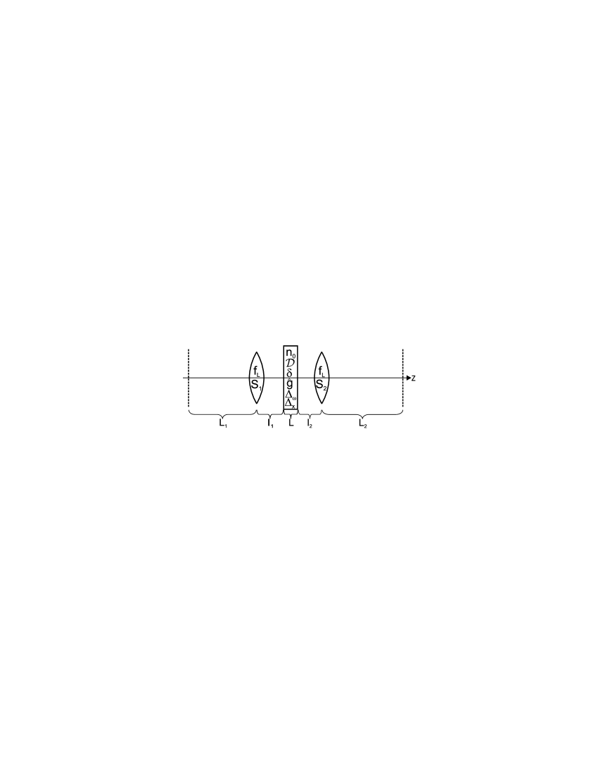
Figure 1: Simplified model of a Kerr-lens mode-locked laser resonator. The end mirrors are represented by dashed lines.

As an example, we choose here the spatiotemporal pulse propagation in a Kerr-lens mode-locked laser resonator. The setup, shown in Fig. 1, consists of a nonlinear Kerr medium and linear resonator arms to its left and right, which contain an element with negative dispersion and a focusing element.jir03 For the resonator arms, we assume a focal length $f_{L}=5\,\mathrm{cm}$ and a group delay dispersion $S_{1}=S_{2}=-75\,\mathrm{fs}^{2}$. For the Kerr medium, the material parameters of Ti:sapphire are used, with $\mathcal{D}=60\,\mathrm{fs}^{2}/\,\mathrm{mm}$, $\delta=k_{0}n_{2I}=0.25\,\mathrm{\mu m}/\,\mathrm{MW}$, $n_{0}=1.76$, $f_{0}=375\,\mathrm{THz}$ and $\mathcal{B}=1/\left(2n_{0}k_{0}\right)=36.2\,\mathrm{nm}$. The lengths in the resonator are given by $L_{1}=80\,\mathrm{cm}$, $L_{2}=110\,\mathrm{cm}$, $l_{1}=5.05\,\mathrm{cm}$, $L=0.25\,\mathrm{cm}$ and $l_{2}=5.2\,\mathrm{cm}$.

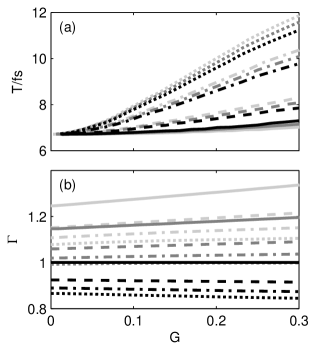
Figure 2: Steady-state pulse solution of the setup shown in Fig. 1 for a fixed intracavity pulse energy of $20\,\mathrm{nJ}$ at the right end mirror. Shown is a) the pulse duration $T$ at right end mirror and b) the stability factor $\Gamma$ as a function of the gain per roundtrip $G$. Results for $\Delta_{\omega}/\left(2\pi\right)=40$, $45$, $56\,\mathrm{THz}$ and $\Delta_{\omega}\rightarrow\infty$ are represented by dotted, dash-dotted, dashed and solid lines, respectively. Transverse gain widths of $\Delta_{x}=10\,\mathrm{\mu m}$, $\Delta_{x}=20\,\mathrm{\mu m}$ and $\Delta_{x}\rightarrow\infty$ are marked by light gray, dark gray and black colors.

In Ref. 4, the Gaussian solutions for the setup in Fig. 1 are obtained taking into account only the energy-conserving effects, i.e., neglecting gain and loss. Here, a Gaussian gain profile in the Kerr medium is added, characterized by the parameters $\hat{g}$, $\Delta_{\omega}$ and $\Delta_{x}=\Delta_{y}$, see Eq. (20). The output coupling is taken into account by normalizing the intracavity pulse energy at the right end mirror to $E=20\,\mathrm{nJ}$. In the following, we examine the dependence of the solution on the gain parameters. Fig. 2 shows the Gaussian pulse duration $T$ at the right end mirror and the stability factor $\Gamma$ as a function of the roundtrip gain $G=\Delta E/E$ for different values of $\Delta_{x}$ and $\Delta_{\omega}$. $\Gamma$ is defined as the ratio between the gain per roundtrip in pulsed and cw operation, $\Gamma=G/G_{\mathrm{cw}}$, where $G_{\mathrm{cw}}$ is the roundtrip gain for the Gaussian steady-state beam solution of the linear resonator. The stability factor serves as an indicator for the suppression of the cw lasing in pulsed operation, a value of $\Gamma>1$ indicating stable pulsed operation.jir03

Fig. 2(a) shows the pulse duration $T$ at the right end mirror. The pulse duration increases for strong spectral gain filtering, i.e., for a strong roundtrip gain $G$ in combination with small gain bandwidth $\Delta_{\omega}$. Also a small transverse gain width $\Delta_{x}$ leads for a fixed value of $G$ to increased spectral filtering, mainly because of the increased peak gain $\hat{g}$. Thus, minimum pulse durations can be obtained in a setup with a small gain and weak outcoupling at the end mirrors. Fig. 2(b) shows the stability parameter $\Gamma$. Due to the high peak power, the pulsed solution experiences self-focusing and thus transverse contraction in the Kerr medium, leading to an increased transverse overlap with the gain. On the other hand, the cw solution is not affected by spectral gain filtering. Thus, $\Gamma$ reaches maximum values for a small transverse gain width $\Delta_{x}$ and a broad gain bandwidth $\Delta_{\omega}$.

The results for vanishing gain, $G\rightarrow 0$, coincide with the ones obtained in Ref. 4, taking into account only the energy-conserving effects. For a small gain of a few percent, the energy-conserving dynamics is still a good approximation, as can be seen from Fig. 2. However, the equations of motion with gain have the distinct advantage that the system is attracted by its stable solutions, while for the energy-conserving equations, additional boundary conditions have to be introduced to find the steady-state solutions.jir03

As pointed out in Ref. 4, higher-order dispersive effects, which are not included here, can considerably affect the pulse shape. In addition, the Gaussian approximation fails for excessive self-focusing and self-phase modulation, as well as strong nonparabolic gain aperturing and filtering. Under extreme conditions, the nonlinear Schrödinger equation itself, as given in Eq. (1), loses its validity.

V CONCLUSION

In conclusion, we have studied the spatial, temporal and spatiotemporal optical propagation in Kerr media with transverse and spectral gain filtering by applying the variational principle. Based on the Kantorovitch method, we derived the Gaussian equations of motion for parabolic and general gain profiles. By reformulating the variational equations as differential equations for the $q$ parameters, we could extract $ABCD$ matrices for the Kerr effect and a general transverse and spectral gain profile. As an example, we studied the steady-state spatiotemporal Gaussian pulse dynamics in a Kerr-lens mode-locked laser resonator.

The equations of motion can be solved efficiently with a standard differential equation solver and allow for a quick simulation of the Gaussian optical propagation through gain media with Kerr nonlinearity. By iterative solution of these equations, the steady-state pulse or beam shape in a laser resonator can be obtained. Further effects, like a parabolic refractive index profile as generated by thermal lensing in a laser rod, can easily be considered by additional $ABCD$ matrices. Gain saturation can be taken into account by complementing the equations of motion with suitable gain saturation equations.

APPENDIX A: DERIVATION OF THE VARIATIONAL EQUATIONS

In this appendix, we derive from Eq. (1) the equations of motion for the spatiotemporal Gaussian pulse parameters, using the Kantorovitch method.cer98 The conservative Lagrangian is given by jir02

$$\mathcal{L} =\frac{\mathrm{i}}{2}\left(U^{\ast}\frac{\partial U}{\partial z}-U\frac{\partial U^{\ast}}{\partial z}\right)+\mathcal{D}\left|\frac{\partial U}{\partial t_{\mathrm{r}}}\right|^{2}-\mathcal{B}\left|\frac{\partial U}{\partial x}\right|^{2}-\mathcal{B}\left|\frac{\partial U}{\partial y}\right|^{2}$$

$$+\frac{\delta}{2}\left|U\right|^{4},$$ (A1)

while the non-conservative process is described by the expression $Q$, given in Eq. (2) and Eq. (11), respectively. For the envelope $U$, we insert the test function Eq. (3). The Euler-Lagrange equations for the real parameter functions $f=A,\phi,T,w_{x},w_{y},b,a_{x},a_{y}$ are then given by cer98

$$\frac{\partial\left\langle\mathcal{L}\right\rangle}{\partial f}-\frac{\mathrm{d}}{\mathrm{d}z}\frac{\partial\left\langle\mathcal{L}\right\rangle}{\partial f^{\prime}}=R_{f},$$ (A2)

with the reduced Lagrangian

$$\left\langle\mathcal{L}\right\rangle=\int_{-\infty}^{\infty}\int_{-\infty}^{\infty}\int_{-\infty}^{\infty}\mathcal{L}\mathrm{d}t_{\mathrm{r}}\mathrm{d}x\mathrm{d}y$$ (A3)

and the non-conservative term

$$R_{f}=2\Re\left\{\int_{-\infty}^{\infty}\int_{-\infty}^{\infty}\int_{-\infty}^{\infty}Q\frac{\partial U^{\ast}}{\partial f}\mathrm{d}t_{\mathrm{r}}\mathrm{d}x\mathrm{d}y\right\}.$$ (A4)

Using the definition of the Fourier transform in Eq. (12) and Parseval’s theorem, we can with $\mathcal{F}_{t}\left\{Q\right\}=\mathrm{i}g\tilde{U}$ express Eq. (A4) as

$$R_{f}=\frac{1}{\pi}\Re\left\{\mathrm{i}\int_{-\infty}^{\infty}\int_{-\infty}^{\infty}\int_{-\infty}^{\infty}g\tilde{U}\frac{\partial\tilde{U}^{\ast}}{\partial f}\mathrm{d}\omega\mathrm{d}x\mathrm{d}y\right\}.$$ (A5)

Since $g$ is real, we have $R_{A}=R_{w_{x}}=R_{w_{y}}=0$. Furthermore, for a parabolic gain profile with the gain term Eq. (2), we obtain

$$R_{\phi}=E\left[2g_{0}-g_{x}w_{x}^{2}-g_{y}w_{y}^{2}-g_{\omega}\Omega^{2}\right],$$ (A6)

$$R_{T}=4g_{\omega}EbT^{-1},$$ (A7)

$$R_{b}=\frac{1}{2}ET^{2}\left[2g_{0}-g_{x}w_{x}^{2}-g_{y}w_{y}^{2}+g_{\omega}\left(T^{-2}-12T^{2}b^{2}\right)\right],$$ (A8)

$$R_{a_{x}}=\frac{1}{2}Ew_{x}^{2}\left[2g_{0}-3g_{x}w_{x}^{2}-g_{y}w_{y}^{2}-g_{\omega}\Omega^{2}\right],$$ (A9)

and a corresponding expression for $R_{a_{y}}$, where the pulse energy is given by

$$E=\pi^{3/2}A^{2}Tw_{x}w_{y}.$$ (A10)

From Eqs. (A6) - (A9), we can extract equations for $g_{\omega}$, $g_{x}$, $g_{y}$ and $g_{0}$,

$$g_{\omega}=R_{T}T/\left(4Eb\right),$$ (A11)

$$g_{x}=\left(R_{\phi}w_{x}^{2}/2-R_{a_{x}}\right)/\left(Ew_{x}^{4}\right),$$ (A12)

$$g_{y}=\left(R_{\phi}w_{y}^{2}/2-R_{a_{y}}\right)/\left(Ew_{y}^{4}\right),$$ (A13)

$$g_{0}=\left(R_{\phi}/E+g_{x}w_{x}^{2}+g_{y}w_{y}^{2}+g_{\omega}\Omega^{2}\right)/2.$$ (A14)

This enables us to express any gain profile formally through effective parabolic gain parameters, which depend on both the gain function and the pulse parameters. Inserting Eq. (A5) into Eqs. (A11) – (A14), we arrive at Eq. (13).

Setting $f=A$ in Eq. (A2) yields

$$\begin{array}[c]{c}-2\phi^{\prime}-\left(b^{\prime}T^{2}+a_{x}^{\prime}w_{x}^{2}+a_{y}^{\prime}w_{y}^{2}\right)+\mathcal{D}\left(\frac{1}{T^{2}}+4b^{2}T^{2}\right)\\ -\mathcal{B}\left(\frac{1}{w_{x}^{2}}+4a_{x}^{2}w_{x}^{2}\right)-\mathcal{B}\left(\frac{1}{w_{y}^{2}}+4a_{y}^{2}w_{y}^{2}\right)+\delta\frac{A^{2}}{\sqrt{2}}=0,\end{array}$$ (A15)

and for $f=\phi$, we get

$$E^{\prime}=E\left[2g_{0}-g_{x}w_{x}^{2}-g_{y}w_{y}^{2}-g_{\omega}\left(\frac{1}{T^{2}}+4b^{2}T^{2}\right)\right].$$ (A16)

The Euler-Lagrange equations for the pulse duration and the beam widths are given by

$$\begin{array}[c]{c}-\phi^{\prime}+\frac{1}{2}\Big{[}-b^{\prime}T^{2}-3a_{x}^{\prime}w_{x}^{2}-a_{y}^{\prime}w_{y}^{2}+\mathcal{D}\left(\frac{1}{T^{2}}+4b^{2}T^{2}\right)\\ -\mathcal{B}\left(-\frac{1}{w_{x}^{2}}+12a_{x}^{2}w_{x}^{2}\right)-\mathcal{B}\left(\frac{1}{w_{y}^{2}}+4a_{y}^{2}w_{y}^{2}\right)\Big{]}+\frac{\delta}{4\sqrt{2}}A^{2}=0,\end{array}$$ (A17)

$$\begin{array}[c]{c}-\phi^{\prime}+\frac{1}{2}\Big{[}-b^{\prime}T^{2}-a_{x}^{\prime}w_{x}^{2}-3a_{y}^{\prime}w_{y}^{2}+\mathcal{D}\left(\frac{1}{T^{2}}+4b^{2}T^{2}\right)\\ -\mathcal{B}\left(\frac{1}{w_{x}^{2}}+4a_{x}^{2}w_{x}^{2}\right)-\mathcal{B}\left(-\frac{1}{w_{y}^{2}}+12a_{y}^{2}w_{y}^{2}\right)\Big{]}+\frac{\delta}{4\sqrt{2}}A^{2}=0,\end{array}$$ (A18)

$$\begin{array}[c]{c}-\phi^{\prime}+\frac{1}{2}\Big{[}-3b^{\prime}T^{2}-a_{x}^{\prime}w_{x}^{2}-a_{y}^{\prime}w_{y}^{2}+\mathcal{D}\left(-\frac{1}{T^{2}}+12b^{2}T^{2}\right)\\ -\mathcal{B}\left(\frac{1}{w_{x}^{2}}+4a_{x}^{2}w_{x}^{2}\right)-\mathcal{B}\left(\frac{1}{w_{y}^{2}}+4a_{y}^{2}w_{y}^{2}\right)\Big{]}+\frac{\delta}{4\sqrt{2}}A^{2}=4g_{\omega}b,\end{array}$$ (A19)

and for the chirp parameters, we obtain

$$\frac{1}{2}E^{\prime}+E\frac{w_{x}^{\prime}}{w_{x}}-4\mathcal{B}Ea_{x}$$

$$=E\left[g_{0}-\frac{3g_{x}}{2}w_{x}^{2}-\frac{g_{y}}{2}w_{y}^{2}-2g_{\omega}\left(\frac{1}{4T^{2}}+b^{2}T^{2}\right)\right],$$ (A20)

$$\frac{1}{2}E^{\prime}+E\frac{w_{y}^{\prime}}{w_{y}}-4\mathcal{B}Ea_{y}$$

$$=E\left[g_{0}-\frac{g_{x}}{2}w_{x}^{2}-\frac{3g_{y}}{2}w_{y}^{2}-2g_{\omega}\left(\frac{1}{4T^{2}}+b^{2}T^{2}\right)\right],$$ (A21)

$$\frac{1}{2}E^{\prime}+E\frac{T^{\prime}}{T}+4\mathcal{D}Eb$$

$$=E\left[g_{0}-\frac{g_{x}}{2}w_{x}^{2}-\frac{g_{y}}{2}w_{y}^{2}+2g_{\omega}\left(\frac{1}{4T^{2}}-3T^{2}b^{2}\right)\right].$$ (A22)

Inserting Eq. (A16) into Eqs. (A20) – (A22) results in Eqs. (5a) and (5b). Multiplying Eqs. (A17), (A18) and (A19) by $2$ and subtracting Eq. (A15) from each equation yields Eqs. (6a) and (6b). Eq. (7) can be obtained from Eq. (A16) by inserting Eqs. (A10), (5a) and (5b). Multiplying Eq. (A15) by a factor of $2\frac{1}{2}$ and subtracting Eqs. (A17), (A18) and (A19) yields Eq. (8).

APPENDIX B: DERIVATION OF THE EQUATIONS FOR THE q PARAMETERS

The spatiotemporal dynamics is described by coupled equations of motion for $q_{x}$, $q_{y}$, $q_{t}$ and $\hat{U}$. Differentiation of Eq. (27) with respect to $z$ yields with Eqs. (5a) and (6a) the differential equation for $q_{p}$,

$$q_{p}^{\prime}=-\left(\frac{2\mathrm{i}g_{p}}{k_{0}}-\frac{2c_{a}\delta}{k_{0}w_{p}^{2}}\left|\hat{U}\right|^{2}\right)q_{p}^{2}+\frac{1}{n_{0}},$$ (B1)

with $p=x,y$ and $w_{p}=\left(k_{0}\Im\left\{q_{p}^{-1}\right\}\right)^{-1/2}$. The differential equation for $q_{t}$ is obtained by differentiating Eq. (28) with respect to $z$ and inserting Eqs. (5b) and (6b):

$$q_{t}^{\prime}=-\frac{2c_{a}\delta}{\omega_{0}T^{2}}\left|\hat{U}\right|^{2}q_{t}^{2}+2\mathcal{D}\omega_{0}+2\mathrm{i}g_{\omega}\omega_{0},$$ (B2)

with $T=\left(-\omega_{0}\Im\left\{q_{t}^{-1}\right\}\right)^{-1/2}$. Differentiating Eq. (4) with respect to $z$ and inserting Eqs. (7) and (8) yields with Eqs. (27) and (28) the equation of motion for the complex amplitude,

$$\frac{\hat{U}^{\prime}}{\hat{U}}=\frac{A^{\prime}}{A}+i\phi^{\prime}=-\frac{\mathcal{B}k_{0}}{q_{x}}-\frac{\mathcal{B}k_{0}}{q_{y}}-\frac{\mathcal{D}\omega_{0}}{q_{t}}-\mathrm{i}\frac{\omega_{0}g_{\omega}}{q_{t}}+g_{0}+\mathrm{i}c_{\phi}\allowbreak\delta\left|\hat{U}\right|^{2}.$$ (B3)

The purely spatial beam propagation, Eq. (29), is described by Eqs. (B1) and (B3) with $\mathcal{D}=g_{\omega}=0$, and the temporal pulse propagation, Eq. (30), is described by Eqs. (B2) and (B3) with $\mathcal{B}=0$. The nonlinearity coefficients are given in Table 1.

In the $q$ parameter formalism, discrete optical elements are represented by $2\times 2$ matrices

$$M_{s}=\left(\begin{array}[c]{cc}A_{s}&B_{s}\\ C_{s}&D_{s}\end{array}\right).$$ (B4)

For the spatiotemporal pulse propagation, each optical element is characterized by three matrices, i.e., $s=x,y,t$. The transformation law for the propagation through an optical element extending from position $z_{1}$ to $z_{2}$,

$$q_{s}\left(z_{2}\right)=\frac{A_{s}q_{s}\left(z_{1}\right)+B_{s}}{C_{s}q_{s}\left(z_{1}\right)+D_{s}},$$ (B5)

is valid for both the spatial and temporal $q$ parameters.sie86 ; dij90 The amplitude at position $z_{2}$ is given by

$$\hat{U}\left(z_{2}\right) =\tau\hat{U}\left(z_{1}\right)\left[A_{x}+B_{x}/q_{x}\left(z_{1}\right)\right]^{-1/2}$$

$$\times\left[A_{y}+B_{y}/q_{y}\left(z_{1}\right)\right]^{-1/2}\left[A_{t}+B_{t}/q_{t}\left(z_{1}\right)\right]^{-1/2}$$ (B6)

for a spatiotemporal Gaussian pulse,

$$\hat{U}\left(z_{2}\right) =\tau\hat{U}\left(z_{1}\right)\left[A_{x}+B_{x}/q_{x}\left(z_{1}\right)\right]^{-1/2}$$

$$\times\left[A_{y}+B_{y}/q_{y}\left(z_{1}\right)\right]^{-1/2}$$ (B7)

for a spatial beam, and

$$\hat{U}\left(z_{2}\right)=\tau\hat{U}\left(z_{1}\right)\left[A_{t}+B_{t}/q_{t}\left(z_{1}\right)\right]^{-1/2}$$ (B8)

for a purely temporal pulse, with the on-axis transmission $\tau=\exp\left(\int\alpha\mathrm{d}z\right)$, where $\alpha$ is the complex on-axis transmission coefficient. The propagation equations Eqs. (B1)–(B3) can be obtained by dividing the Kerr medium into small sections of length $\delta z$, and representing each section by $ABCD$ matrices of the form Eq. (33). From Eqs. (B5) and (B6), we obtain

$$q_{s}\left(z+\delta z\right)=\frac{q_{s}\left(z\right)+B_{s}^{\prime}\delta z}{q_{s}C_{s}^{\prime}\delta z+1}\approx-q_{s}^{2}\left(z\right)C_{s}^{\prime}\delta z+q_{s}\left(z\right)+B_{s}^{\prime}\delta z$$ (B9)

and

$$\hat{U}\left(z+\delta z\right) =\hat{U}\left(z\right)\exp\left(\alpha\delta z\right)\left(1+B_{x}^{\prime}\delta z/q_{x}\right)^{-1/2}$$

$$\times\left(1+B_{y}^{\prime}\delta z/q_{y}\right)^{-1/2}\left(1+B_{t}^{\prime}\delta z/q_{t}\right)^{-1/2}$$

$$\approx\hat{U}\left(z\right)\left(1-\frac{B_{x}^{\prime}\delta z}{2q_{x}}-\frac{B_{y}^{\prime}\delta z}{2q_{y}}-\frac{B_{t}^{\prime}\delta z}{2q_{t}}+\alpha\delta z\right).$$ (B10)

In the limit $\delta z\rightarrow 0$, this results in Eqs. (31) and (32). Comparison with Eqs. (B1), (B2), and (B3) yields the elements Eq. (34) and the $\alpha$ given in Eq. (35). The equations for the purely spatial or temporal dynamics can be derived in an analogous manner.

References

• (1) M. Manousakis, S. Droulias, P. Papagiannis, and K. Hizanidis, “Propagation of chirped solitary pulses in optical transmission lines: perturbed variational approach,” Opt. Commun. 213, 293–299 (2002).
• (2) I. P. Christov and V. D. Stoev, “Kerr-lens mode-locked laser model: role of space-time effects,” J. Opt. Soc. Am. B 15, 1960–1966 (1998).
• (3) V. P. Kalosha, M. Müller, J. Herrmann, and S. Gatz, “Spatiotemporal model of femtosecond pulse generation in Kerr-lens mode-locked solid-state lasers,” J. Opt. Soc. Am. B 15, 535–550 (1998).
• (4) C. Jirauschek, F. X. Kärtner, and U. Morgner, “Spatiotemporal Gaussian pulse dynamics in Kerr-lens mode-locked lasers,” J. Opt. Soc. Am. B 20, 1356–1368 (2003).
• (5) D. Anderson and M. Bonnedal, “Variational approach to nonlinear self-focusing of Gaussian laser beams,” Phys. Fluids 22, 105–109 (1979).
• (6) D. Anderson, M. Bonnedal, and M. Lisak, “Self-trapped cylindrical laser beams,” Phys. Fluids 22, 1838–1840 (1979).
• (7) D. Anderson, “Variational approach to nonlinear pulse propagation in optical fibers,” Phys. Rev. A 27, 3135–3145 (1983).
• (8) M. Desaix, D. Anderson, and M. Lisak, “Variational approach to collapse of optical pulses,” J. Opt. Soc. Am. B 8, 2082–2086 (1991).
• (9) C. Jirauschek, U. Morgner, and F. X. Kärtner, “Variational analysis of spatio-temporal pulse dynamics in dispersive Kerr media,” J. Opt. Soc. Am. B 19, 1716–1721 (2002).
• (10) D. J. Kaup and B. A. Malomed, “The variational principle for nonlinear waves in dissipative systems,” Physica D 87, 155–159 (1995).
• (11) F. Riewe, “Nonconservative Lagrangian and Hamiltonian mechanics,” Phys. Rev. E 53, 1890–1899 (1996).
• (12) S. C. Cerda, S. B. Cavalcanti, and J. M. Hickmann, “A variational approach of nonlinear dissipative pulse propagation,” Eur. Phys. J. D  1, 313–316 (1998).
• (13) D. Anderson, F. Cattani, and M. Lisak, “On the Pereira-Stenflo solitons,” Physica Scripta T82, 32–35 (1999).
• (14) N. Aközbek, C. M. Bowden, A. Talebpour, and S. L. Chin, “Femtosecond pulse propagation in air: Variational analysis,” Phys. Rev. E 61, 4540–4549 (2000).
• (15) A. E. Siegman, Lasers (University Science Books, Mill Valley, California, 1986).
• (16) S. P. Dijaili, A. Dienes, and J. S. Smith, “ABCD matrices for dispersive pulse propagation,” IEEE J. Quantum Electron. 26, 1158–1164 (1990).
• (17) Y. Chen and H. A. Haus, “Dispersion-managed solitons in the net positive dispersion regime,” J. Opt. Soc. Am. B 16, 24–30 (1999).
• (18) Y. Chen, F. X. Kärtner, U. Morgner, S. H. Cho, H. A. Haus, E. P. Ippen, and J. G. Fujimoto, “Dispersion-managed mode locking,” J. Opt. Soc. Am. B 16, 1999–2004 (1999).
• (19) A. Penzkofer, M. Wittmann, M. Lorenz, E. Siegert, and S. Macnamara, “Kerr lens effects in a folded-cavity four-mirror linear resonator,” Opt. Quantum Electron. 28, 423–442 (1996).
• (20) V. Magni, G. Cerullo, and S. De Silvestri, “ABCD matrix analysis of propagation of gaussian beams through Kerr media,” Opt. Commun. 96, 348–355 (1993).
• (21) M. A. Larotonda and A. A. Hnilo, “Short laser pulse parameters in a nonlinear medium: different approximations of the ray-pulse matrix,” Opt. Commun. 183, 207–213 (2000).
• (22) A. G. Kostenbauder, “Ray-Pulse Matrices: A Rational Treatment for Dispersive Optical Systems,” IEEE J. Quantum Electron. 26, 1148–1157 (1990).
• (23) J. L. A. Chilla and O. E. Martínez, “Spatial-temporal analysis of the self-mode-locked Ti: sapphire laser,” J. Opt. Soc. Am. B 10, 638–643 (1993).
• (24) M. Nakazawa, H. Kubota, A. Sahara, and K. Tamura, “Time-domain ABCD matrix formalism for laser mode-locking and optical pulse transmission,” IEEE J. Quantum Electron. 34, 1075–1081 (1998).
• (25) B. H. Kolner and M. Nazarathy, “Temporal imaging with a time lens,” Opt. Lett. 14, 630–632 (1989).
• (26) E. J. Grace, G. H. C. New, and P. M. W. French, “Simple ABCD matrix treatment for transversely varying saturable gain,” Opt. Lett. 26, 1776–1778 (2001).