Double-component convection due to different boundary conditions with broken reflection symmetry for a component

Abstract

Onset of two- (2D) and three-dimensional (3D) double-component convection due to different boundary conditions is studied in a diversely oriented infinite slot with broken symmetry between the slot conditions for a component. The main focus is on the two compensating background gradients. Different component conditions at one slot boundary (the distinction boundary) are considered with such a joint component condition at the other (the similarity boundary) as can be both of the flux ($\eta=\chi=0$) and of the fixed-value ($\eta=\chi=1$) type. Also examined are such component conditions at the second boundary (the inverse boundary) as differ from each other inversely to the distinction boundary ($\eta=0$ and $\chi=1$). In the horizontal slot with inviscid fluid and oscillatory primary instability for $\eta=\chi$, the most unstable wavelength being infinite at $\eta=\chi=0$ is rendered finite by flux-component (solute) diffusion at the similarity boundary when $\eta=\chi=1$. In the viscous fluid, however, such a diffusion of both components enhances the instability efficiency compared to $\eta=\chi=0$. With all above types of the broken symmetry, small-amplitude convection in viscous fluid remains of an oscillatory nature for any slot orientation other than the inversely-stratified horizontal one. For $\eta=0$ and $\chi=1$, such a universality also involves various abrupt changes in the marginal-stability curves. These come from respectively identified mechanisms of switching between dissimilar oscillatory patterns. In inviscid fluid, such changes emerge with the zero instability threshold. Some of these abrupt changes give rise to new mechanisms for three-dimensionality of the instability. Such a mechanism arises in viscous fluid for $\eta=\chi=0$ as well. It comes with multiplicity and isolated existence of as well as hysteresis between solutions of the linear stability equations. Both the hysteresis region and the other above abrupt 3D changes are described in terms of analogy between the effect of $G=k_{y}/k$, the ratio of the 2D and 3D wave numbers, and that of a 2D ratio between two gravity components. Other revealed 3D effects are attributable to new manifestations of their general mechanism identified by Tsitverblit [Ann. Phys. 322 (2007) 1727]. Apart from dissipation, this mechanism also arises from solute diffusion at the similarity boundary for $\eta=\chi=1$ and from differential gradient diffusion at either boundary for $\eta=0$ and $\chi=1$. It also incorporates change of the nature of instability from steady to oscillatory. In the context of the steady linear instability, differential gradient diffusion is shown to be more effective at the stress-free slot boundary than at the no-slip one. Although the mechanism of finite-amplitude steady convection revealed by Tsitverblit [Phys. Lett. A 329 (2004) 445] is most effective herein for $\eta=\chi=1$, its manifestation remains well-pronounced for $\eta=\chi<0.5$ as well. Relevance of this mechanism to abrupt climate change is thus discussed.

1 Introduction

This work addresses manifestations of a broken symmetry in double-component, buoyancy-driven convection resulting from the boundary conditions for one component being different from those for the other. Such convection has recently been identified as a fundamental class of pattern-forming hydrodynamic instabilities. The objective of this study is to establish the understanding of these instabilities for problems where a major element of previously assumed reflection symmetry is absent: the distinction between the components coming from one boundary of the fluid domain is not reflected at the other.

The paradigm of double-component convection in pure fluid first arose in the context of conventional double-diffusive convection. This is a class of phenomena resulting from the effects of unequal diffusion coefficients of two density-affecting components [1, 2, 3]. Among numerous natural science and technology applications of this subject emphasized in its initial reviews [4], particular attention has subsequently been focused on small-scale oceanography [5], ordinary evolution of stars [6], geology [7], geodynamo [8], and crystal growth [9]. Recently, relevance of double-component convection has also been highlighted for the dynamics of proto-neutron stars during core-collapse supernova explosions [10], as well as for colloidal suspensions [11], and soap films [12].

Since the boundary conditions for one component are generically expected to be different from those for the other, the effects of such different component conditions are relevant to all the above areas of application of conventional double-diffusive convection. However, these effects also apply to an eddy-diffusion description of large-scale environmental and turbulent processes, where disparity between the component diffusivities may be practically negligible. Such processes range from Langmuir circulations [13, 14] to the global ocean thermohaline circulation [15, 16, 17, 18, 19, 20, 21] and associated climate change [22, 23, 24]. In addition, convective flows are commonly used in fundamental studies of transition to turbulence [25] and nonlinear pattern formation [26].

One major subclass of double-component instabilities arising from the effects of different boundary conditions comprises phenomena whose nature is conceptually analogous to the classical double-diffusion [1, 2, 3]. Differential diffusion caused by unequal component gradients forming in perturbed state due to the different boundary conditions (differential gradient diffusion) triggers convection analogously to the effects of disparate diffusivities. Generalizing the idea in [27], such analogy has been introduced in [28, 29, 30, 31] and scrutinized in [32].

In particular, the nature of an oscillatory instability highlighted in [27] and analyzed in [32] is analogous to that in the diffusive regime of the classical double-diffusion [1, 2]. The viscous problem with the stratification inverse to that in [27] also gives rise to a mechanism of steady convection [28, 29] that is conceptually analogous to the finger instability in conventional double-diffusive convection [1]. This mechanism generates Langmuir circulations in the presence of a stable background density stratification [13, 14]. For the component conditions being different only at one boundary and the other boundary being infinitely distant, the stratification considered in [28, 29] has been more recently treated in [33].

For two horizontal component gradients arising in a laterally heated stably stratified slot, the effect of different boundary conditions [30] is also analogous to the classical double-diffusion [34]. As in conventional double-diffusive convection [35], in addition, steady finite-amplitude instability is triggered from the state of rest by different sidewall boundary conditions for two compensating horizontal gradients of the components [31]. Arising without the linear steady instability of the conduction state [36], however, such a finite-amplitude manifestation of convection in [31] also exposes an oscillatory linear instability whose nature is underlain by differential gradient diffusion [32].

Effects of different boundary conditions also extend beyond the instabilities being due to differential gradient diffusion. As reported in [37], finite-amplitude steady convection arises well before onset of the respective linear instability in the viscous version of the problem in [27]. It is then generated by the feedback coming from nonlinear Rayleigh—Benard convection, despite the stabilizing role of differential gradient diffusion. Potential relevance of such a mechanism to abruptly changing global environmental phenomena [15, 16, 20, 21, 22, 23, 24] makes its examination under more realistic conditions particularly important.

In the above studies of slot double-component convection due to different boundary conditions, the condition for either component at one slot boundary has been identical to the respective condition at the other. The considered problems have thus been reflectionally symmetric across the slot. Being an important initial simplification, the reflection symmetry is however unlikely to be maintained in real-world applications of the effects of different boundary conditions. This is also particularly relevant if the component-dependent forces other than the buoyancy forces are considered, as suggested in [32, 37].

Manifestation of physical laws in the absence of certain symmetries underlying them could make both the laws themselves and their broken symmetries hardly recognizable. This has been repeatedly illustrated in elementary particle physics and cosmological theories of unification of fundamental forces [38]. Another illustration is the irreversibility in statistical mechanics [39] and its generalized (symmetric) interpretation [40]. In geophysics, the global ocean thermohaline circulation also involves asymmetries [17, 18, 19, 41]. Clarification of the nature of such asymmetries is viewed as critical for understanding past and predicting future major changes of the Earth climate [22].

For classic hydrodynamic instabilities, one can refer to the structure of multiple steady flows in the Taylor experiment [42], where translation invariance is broken by end walls. Complex as it becomes when the cylinder aspect ratio is increased [43], this structure is not expected to transform into that in the translationally invariant problem even when the aspect ratio tends to infinity [44]. In addition, if oscillatory instability arises in a flow that is both reflectionally and translationally symmetric, the corresponding Hopf bifurcation would give rise to two respectively symmetric oscillatory branches [45]. Elimination of one of the symmetries from such a system could thus have a major effect on the structure and nature of its nonequilibrium flows.

The general objective of the present work has been to provide a comprehensive insight into the effects of different boundary conditions in a slot where the previously assumed boundary conditions symmetry is broken. In a class of such problems, the component conditions are different only at one slot boundary (hereafter, the distinction boundary). These problems are addressed for such a joint component condition at the other (hereafter, the similarity boundary) as can range from the flux to the fixed-value type. Being referred to as the inverse boundary, this other boundary is also considered with such different component conditions as are prescribed oppositely to the distinction boundary.

Among consequences of the broken symmetry is a universality of oscillatory manifestation of the effects of different boundary conditions in viscous fluid. For all above types of the boundary conditions, the steady linear instability analogous to that in [28, 29] transforms into an oscillatory one for any slot deviation from the horizontal orientation. Three-dimensionality and, eventually, an isolated nonlinearity, hysteresis, and other abrupt changes in such oscillatory-linear-instability curves are underlain by the respective horizontal-slot steady instabilities. Other new three-dimensional effects come from abruptly emerging zero thresholds of the inviscid oscillatory instability. Most pronouncedly manifested herein for the fixed-value similarity boundary, the mechanism of finite-amplitude steady convection [37] is also relevant when the component condition at this boundary is closer to the flux than to the fixed-value type.

2 The problem formulation and solution procedures

2.1 The problem and governing equations

A general case of the considered problem is illustrated in Fig. 1, where $\theta$ ($>0$ in Fig. 1) is the angle between the direction opposite to the gravity and that of the across-slot coordinate axis in an infinite slot with pure fluid. The component gradients in Fig. 1 are represented by the Rayleigh numbers $Ra=g\alpha\Delta\overline{T}d^{3}/\kappa\nu$ and $Ra^{s}=-g\beta(\partial\overline{s}/\partial\overline{x})d^{4}/\kappa\nu\equiv\mu Ra$. Here, $\overline{x}$ is the (dimensional) across-slot coordinate, $d$ is the width of the slot, $\Delta\overline{T}$ is the (dimensional) conduction-state difference between the values of temperature (the component with the fixed-value condition at the distinction boundary) at the boundaries with smaller and larger across-slot coordinates, $\partial\overline{s}/\partial\overline{x}$ is the (dimensional) derivative of solute concentration, the component with the flux condition, at the distinction boundary, $\alpha$ is the coefficient of thermal expansion, $\beta$ is the coefficient of the density variation due to the variation of solute concentration, $g$ is the gravitational acceleration, $\nu$ is the kinematic viscosity, and $\kappa=\kappa_{T}=\kappa_{S}$ is the diffusivity of both components. The bar means that the respective variable is dimensional. Unless explicitly stated otherwise, $Ra>0$ and $Ra^{s}>0$ as well as $\mu=1$ (i.e., the compensating background gradients) are assumed.

As in [28, 29, 30, 31, 32, 37], the component diffusivities are set equal to eliminate the classical double-diffusive effects. Such an approach has also been adopted in most studies of conventional double-diffusive convection, where the components with unequal diffusivities were not distinguished from each other in terms of their boundary conditions. In principle, equal diffusivities can also be experimentally modeled with two solutes [46]. The Prandtl number, which would then be significantly different from the present $Pr=6.7$, is not expected to have a qualitative effect on the main results and physical interpretations discussed herein. Equal diffusivities could be interpreted as eddy transport coefficients as well, as in [13, 14, 19]. $Pr=6.7$ is then also within the range of realistic values for all diffusion coefficients to be of the eddy type.

For facilitating comparison of the results for an inclined or vertical slot with those for a horizontal slot, this study is focused on the exactly compensating background gradients ($\mu=1$). This eliminates the along-slot motion arising when the slot orientation differs from horizontal. In particular, transformation of the oscillatory instabilities at $\theta\in[0,\pi)$ into the respective steady instabilities at $\theta=\pi$ can thus be analyzed in the framework of the effects of different boundary conditions alone. Such compensating gradients have also been adopted in many studies of conventional double-diffusive convection [35, 47].

The equations describing the two-dimensional (2D) problem in Fig. 1 can be written as follows:

$$\frac{\partial\zeta}{\partial\tau}+\frac{\partial\psi}{\partial x}\frac{\partial\zeta}{\partial y}-\frac{\partial\psi}{\partial y}\frac{\partial\zeta}{\partial x}=\frac{1}{Pr}(\frac{\partial t}{\partial x}-\frac{\partial s}{\partial x})\sin\theta-$$

$$\frac{1}{Pr}(\frac{\partial t}{\partial y}-\frac{\partial s}{\partial y})\cos\theta+\frac{\partial^{2}\zeta}{\partial x^{2}}+\frac{\partial^{2}\zeta}{\partial y^{2}},$$ (1)

$$\zeta=\frac{\partial^{2}\psi}{\partial x^{2}}+\frac{\partial^{2}\psi}{\partial y^{2}},$$ (2)

$$\frac{\partial\xi_{i}}{\partial\tau}+\frac{\partial\psi}{\partial x}\frac{\partial\xi_{i}}{\partial y}-\frac{\partial\psi}{\partial y}\frac{\partial\xi_{i}}{\partial x}=\frac{1}{Pr}(\frac{\partial^{2}\xi_{i}}{\partial x^{2}}+\frac{\partial^{2}\xi_{i}}{\partial y^{2}}),\hskip 28.45274pti=1,2.$$ (3)

Here $\xi_{1}$ and $\xi_{2}$ stand for $t$ and $s$, the across-slot, $u$, and along-slot, $v$, velocities are

$$u=-\frac{\partial\psi}{\partial y},\;\;\;\;\;\;\;v=\frac{\partial\psi}{\partial x},$$

vorticity

$$\zeta=\frac{\partial v}{\partial x}-\frac{\partial u}{\partial y},$$

$Pr=\nu/\kappa$ is the Prandtl number, $\tau$ is the time, $x\in(-1/2,1/2)$, $y\in(-\lambda/2,\lambda/2)$, and $\lambda=\overline{\lambda}/d$ is the specified along-slot period.

Eqs. (1)—(3) are considered along with wall boundary conditions for $\zeta$ and $\psi$

$$\zeta=\gamma_{\pm}\frac{\partial^{2}\psi}{\partial x^{2}},\;\;\;\;\;\psi=0\;\;\;\;\;(x=\pm 1/2,\,-\lambda/2<y<\lambda/2),$$ (4)

where $\gamma_{\pm}=1$ and $\gamma_{\pm}=0$ stand for the no-slip and stress-free boundaries, respectively, as well as with wall boundary conditions for $t$ and $s$

$$t=\frac{Ra}{2}\;\;\;\;\;\;\;\;\;\;\;\;\;\;\;\;\;\;\;\;\;\;\;\;\;\;\;\;\;\;\;(x=-1/2,\;-\lambda/2<y<\lambda/2),$$ (5)

$$\frac{\partial s}{\partial x}=-\mu Ra=-Ra^{s}\;\;\;\;\;(x=-1/2,\;\;-\lambda/2<y<\lambda/2,\;\;y\neq 0),$$

$$(1-\chi_{0})(s-\frac{Ra^{s}}{2})+\chi_{0}(\frac{\partial s}{\partial x}+Ra^{s})=0\;\;\;\;\;\;\;(x=-1/2,\;\;y=0),$$ (6)

$$(1-\eta)(\frac{\partial t}{\partial x}+Ra)+\eta(t+\frac{Ra}{2})=0\;\;\;\;(x=1/2,\;\;-\lambda/2<y<\lambda/2),$$ (7)

$$(1-\chi)(\frac{\partial s}{\partial x}+Ra^{s})+\chi(s+\frac{Ra^{s}}{2})=0\;\;(x=1/2,\;-\lambda/2<y<\lambda/2,\;y\neq 0),$$

$$(1-\chi_{1})(\frac{\partial s}{\partial x}+\frac{Ra^{s}}{2})+\chi_{1}(s+\frac{Ra^{s}}{2})=0\;\;\;\;\;\;(x=1/2,\;\;y=0)$$ (8)

and periodic boundary conditions in the along-slot direction

$$\xi(x,\lambda/2)=\xi(x,-\lambda/2),\;\;\;\;\;\;\frac{\partial\xi(x,\lambda/2)}{\partial y}=\frac{\partial\xi(x,-\lambda/2)}{\partial y}$$

$$(-1/2<x<1/2).$$ (9)

Here $\xi$ stands for $\zeta$, $\psi$, $t$, and $s$, $\chi_{0}=0$ for $\chi<1$ or in all simulations of the linear stability for $\theta=0$ and $\chi_{0}=1$ otherwise, $\chi_{1}=1$ for $\theta=\pi/2$ and $\chi_{1}=\chi$ for $\theta=0$. In the present study, $Pr=6.7$ as well as either $\eta=\chi=0$ or $\eta=\chi=1$ or $\eta=0$ and $\chi=1$ unless $\eta=\chi\in(0,1)$ is specified for $\theta=0$.

In (6) and (8), specification of the middle values of $s$ identifies the solute scale and the solution phase for $\eta=\chi<1$ at $\theta=0$, symmetrically fixes the solute scale in the temporal simulations for $\eta=\chi=0$ at $\theta=\pi/2$, and fixes the solution phase in such simulations for $\eta=\chi=1$ at $\theta=0$. The phase of a nontrivial steady solution for $\theta=0$ when $\chi=1$ and either $\eta=1$ or $\eta=0$ was selected by continuation in $\chi$ and $\eta$ from the progenitor of such a solution at $\eta=1$ and $\chi=0$ in [32, 37], where the phase and the solute scale were fixed at the periodic condition boundaries. The latter approach becomes inconsistent with the natural solute scale specification in the nontrivial steady solutions for $\chi=1$. It also leads to early spurious oscillatory instabilities of the background state for $\eta=\chi=0$ at $\theta=0$. It was not thus employed in the reported results.

In boundary conditions (4)—(9), switching the distinction and the other boundary designations in Fig. 1 is equivalent to transformation

$$(x,y,\theta,Ra,Ra^{s})^{T}\mapsto(-x,-y,\theta+\pi,-Ra,-Ra^{s})^{T}.$$ (10)

Since Eqs. (1)—(3) are invariant under (10), one can consider only such slot orientation to the gravity as is depicted in Fig. 1.

Discretized by central finite differences, the steady version of Eqs. (1)—(3) and boundary conditions (4)—(9) was treated with the Euler—Newton and Keller arclength [48] continuation algorithms to trace out bifurcating branches [30]. These algorithms were based on the Harwell MA32 Fortran routine. The along-slot period $\lambda=2$ was prescribed. The grid with $33$ nodes in the across-slot direction was used in the computations [$nx\times\lambda(nx+1)$ with $nx=33$], as in [28, 29, 30, 31, 32, 37]. As already indicated, temporal behavior of the linearized version of Eqs. (1)—(3) and boundary conditions (4)—(9) was also examined near the onset of oscillatory instability of the conduction state. Such an examination was conducted with the implicit method and time step $\delta\tau=0.05$.

2.2 Linear stability calculations

With the state of rest being the background flow for $\mu=1$, the Fourier mode of a three-dimensional (3D) marginally unstable oscillatory perturbation with angular frequency $\omega$ and a wave number $k=(k_{y}^{2}+k_{z}^{2})^{1/2}$ having $y$ and $z$ components $k_{y}$ and $k_{z}$, respectively, can be written as

$$[u^{\prime}(x),t^{\prime}(x),s^{\prime}(x)]^{T}e^{i(\omega\tau\pm k_{y}y+k_{z}z)}+cc.$$ (11)

(The $z$-axis is orthogonal to the $x$–$y$ plane in Fig. 1 and is directed towards the reader.) Here $[u^{\prime}(x),t^{\prime}(x),s^{\prime}(x)]^{T}$ is the Fourier-mode part depending on the across-slot coordinate alone, the prime near a flow variable denotes such part in the perturbation of the variable. Expression (11) has been introduced into the linearized 3D governing equations that were nondimensionalized consistently with (2D) Eqs. (1)—(3) and rewritten in terms of across-slot velocity $u$, temperature $t$, and solute concentration $s$. This leads to:

$$(\frac{d^{2}}{dx^{2}}-k^{2})(\frac{d^{2}}{dx^{2}}-k^{2}-i\omega)\tilde{u}=$$

$$\mp Ra[iGk\frac{d}{dx}(\tilde{t}-\tilde{s})\sin\theta\pm k^{2}(\tilde{t}-\tilde{s})\cos\theta],$$ (12)

$$(\frac{d^{2}}{dx^{2}}-k^{2}-i\omega Pr)\tilde{\xi}_{i}=\tilde{u},\hskip 28.45274pti=1,2,$$ (13)

where $G\equiv k_{y}/k$, $\tilde{u}=-u^{\prime}Pr$, $\tilde{\xi}_{1}\equiv\tilde{t}=t^{\prime}/Ra$, and $\tilde{\xi}_{2}\equiv\tilde{s}=s^{\prime}/Ra^{s}$ ($Ra^{s}=Ra$).

The variable $\tilde{u}$ is subject to boundary conditions

$$\tilde{u}=(1-\gamma_{\pm})\frac{d^{2}\tilde{u}}{dx^{2}}+\gamma_{\pm}\frac{d\tilde{u}}{dx}=0\;\;\;\;\;\;\;\;(x=\pm 1/2),$$ (14)

where $\gamma_{+}=0,1$ and $\gamma_{-}=0,1$. Unless the values of $\gamma_{\pm}$ are explicitly given, the boundaries are assumed to be either both stress-free ($\gamma_{\pm}=0$) or both no-slip ($\gamma_{\pm}=1$). Such boundary conditions for $\tilde{u}$ are used along with

$$\tilde{t}=\frac{d\tilde{s}}{dx}=0\;\;\;\;(x=-1/2)$$ (15)

and

$$(1-\eta)\frac{d\tilde{t}}{dx}+\eta\tilde{t}=(1-\chi)\frac{d\tilde{s}}{dx}+\chi\tilde{s}=0\;\;\;\;(x=1/2),$$ (16)

where either $\eta=\chi=0$ or $\eta=\chi=1$ or $\eta=0$ and $\chi=1$.

Let $[\tilde{u}(x),\tilde{t}(x),\tilde{s}(x)]^{T}$ be a solution of the $e^{i(\omega\tau+k_{y}y+k_{z}z)}$-version of Eqs. (12) and (13) and boundary conditions (14)—(16) at some $Ra_{c}$ and $\omega_{c}$ for a value of $\theta$ and the orientation of $x$ and $y$ axes as in Fig. 1. If $(x,y,\theta)^{T}$ is transformed into $(-x,-y,\theta+\pi)^{T}$ in boundary conditions (14)—(16) (i.e., if the distinction and the other boundary designations in Fig. 1 are switched), $[\tilde{u}(x),\tilde{t}(x),\tilde{s}(x)]^{T}$ would then be a solution of the $e^{i(\omega\tau-k_{y}y+k_{z}z)}$-version of Eqs. (12) and (13) at $-Ra_{c}$ and the same $\omega_{c}$. This symmetry is related to invariance (10) of Eqs. (1)—(3). It allows to consider only one orientation of the slot boundaries to the gravity, provided that both signs of $k_{y}$ in (11) are taken into account.

For examination of the linear stability of the conduction state in inviscid fluid,

$$i\omega(\frac{d^{2}}{dx^{2}}-k^{2})\tilde{u}=Ra[\pm iGk\frac{d}{dx}(\tilde{t}-\tilde{s})\sin\theta+k^{2}(\tilde{t}-\tilde{s})\cos\theta]$$ (17)

was used along with

$$(\frac{d^{2}}{dx^{2}}-k^{2}-i\omega)\tilde{\xi}_{i}=\tilde{u},\hskip 28.45274pti=1,2,$$ (18)

where the Rayleigh numbers are defined as $Ra=g\alpha\Delta\overline{T}d^{3}/\kappa^{2}$ and $Ra^{s}=-g\beta(\partial\overline{s}/\partial\overline{x})d^{4}/\kappa^{2}=Ra$. Here $\omega$ is nondimensionalized with $\kappa/d^{2}$ as opposed to $\nu/d^{2}$ in Eqs. (12) and (13). The definitions of $Ra$, $Ra^{s}$, and $\omega$ for inviscid fluid are then different from the respective definitions for viscous fluid. Such definitions are thus used below according to the type of fluid in question.

The boundary conditions for inviscid fluid are

$$\tilde{u}=0\;\;\;\;(x=\pm 1/2)$$ (19)

along with (15) and (16).

For $\eta=0$ and $\chi=1$, Eqs. (12) and (13) along with boundary conditions (14)—(16) for $\gamma_{-}=\gamma_{+}$ as well as Eqs. (17) and (18) and boundary conditions (15), (16), and (19) are invariant under transformation

$$[\tilde{u}(x),\tilde{t}(x),\tilde{s}(x),\theta]^{T}\mapsto[\tilde{u}(-x),\tilde{s}(-x),\tilde{t}(-x),\pi-\theta]^{T}.$$ (20)

For $\eta=0$ and $\chi=1$, therefore, $\theta\in[0,\pi/2]$ and $\theta\in[\pi/2,\pi]$ are equivalent in the context of (20). For $Ra\neq Ra^{s}$ at $\theta=0$ and $\theta=\pi$ as well as for $\gamma_{-}\neq\gamma_{+}$ in viscous fluid, such an equivalence also implies additional transformations. These are specified when the respective results are discussed below.

The inviscid problem in a horizontal slot was also examined for the $Ra$ and $Ra^{s}$ being independent of each other. In particular,

$$i\omega(\frac{d^{2}}{dx^{2}}-k^{2})\tilde{u}=k^{2}(Ra\tilde{t}-Ra^{s}\tilde{s})\cos\theta$$ (21)

was considered along with Eqs. (18) and boundary conditions (15), (16), and (19). This was done at given values of $Ra^{s}$ and $\theta=0$ for any of the pairs of $\eta$ and $\chi$ specified above. As already indicated, such a problem for $\eta=0$ and $\chi=1$ is equivalent to that with the fixed values of $Ra$ at $\theta=\pi$.

For fixed $k_{y}$ and $k_{z}$, $Ra_{c}$ and $\omega_{c}$ are found by searching in the $Ra$–$\omega$ domain for the smallest $Ra$ at which the complex matrix resulting from the application of boundary conditions (14)—(16) to the general solution of Eqs. (12) and (13) is singular. The same procedure is applied to the general solution either of Eqs. (17) and (18) or of Eqs. (18) and (21) for $\theta=0$ with boundary conditions (15), (16), and (19). NAG Fortran routines were employed for this purpose.

Once $Ra_{c}(k_{y}^{0})$ and $\omega_{c}(k_{y}^{0})$ have been found for a given $k_{y}^{0}$ and fixed $k_{z}$, the corresponding values of these parameters, $Ra_{c}(k_{y})$ and $\omega_{c}(k_{y})$, at a nearby $k_{y}$ are computed by the Euler—Newton continuation method. The latter is applied to the solution of equation

$$F[Ra(k_{y}),\omega(k_{y}),k_{y},k_{z}]=0,$$ (22)

where $F[Ra(k_{y}),\omega(k_{y}),k_{y},k_{z}]$ stands for the (complex) determinant of the matrix resulting from the application of boundary conditions (14)—(16) or (15), (16), and (19) to the general solution of the respective set of differential equations. Due to the use of standard Fortran routines, the Jacobian of $\{Re[F(Ra,\omega,k_{y},k_{z})],Im[F(Ra,\omega,k_{y},k_{z})]\}^{T}$ (with respect to $Ra$ and $\omega$) and $\partial{F(Ra,\omega,k_{y},k_{z})}/\partial{k_{y}}$ were computed with numerical differentiation. When 3D effects were anticipated, they were studied by repeating the procedure just described for different $k_{z}\geq 0$.

Since the linear instability to steady disturbances in viscous fluid was found to arise only in a horizontal slot, the corresponding problem is discussed in the 2D framework alone. For the compensating background gradients, in particular, $\omega=0$ and $k_{y}=k$ are set in Eqs. (12) and (13) to obtain

$$(\frac{d^{2}}{dx^{2}}-k^{2})^{2}\tilde{u}=-Ra[ik\frac{d}{dx}(\tilde{t}-\tilde{s})\sin\theta+k^{2}(\tilde{t}-\tilde{s})\cos\theta],$$ (23)

$$(\frac{d^{2}}{dx^{2}}-k^{2})\tilde{\xi}_{i}=\tilde{u},\hskip 28.45274pti=1,2.$$ (24)

At $\theta=\pi$, the marginal-stability boundaries described by Eqs. (23) and (24) and boundary conditions (14)—(16) were found for any of the above pairs of $\eta$ and $\chi$. For $\eta=0$ and $\chi=1$, they were found at $\theta=0$ as well, in view of (20). For $\theta=0$ and $\theta=\pi$, steady linear instability was also examined for the $Ra$ and $Ra^{s}$ being independent of each other:

$$(\frac{d^{2}}{dx^{2}}-k^{2})^{2}\tilde{u}=-k^{2}(Ra\tilde{t}-Ra^{s}\tilde{s})\cos\theta$$ (25)

and Eqs. (24) were used either at $\theta=\pi$ for any of the pairs of $\eta$ and $\chi$ specified above or at $\theta=0$ for $\eta=0$ and $\chi=1$ alone.

The general solution either of Eqs. (23) and (24) or of Eqs. (24) and (25) is obtained analytically. Boundary conditions (14)—(16) are then applied to such a general solution. In the former case, the smallest $Ra$, $Ra_{c}(k)$, at which the resulting matrix becomes singular is searched for at different $k$ (and found only for $\theta=\pi$, besides $\theta=0$ when $\eta=0$ and $\chi=1$). In the latter case, such a search yields either the smallest $Ra^{s}$, $Ra^{s}_{c}(k)$, for a fixed $Ra$ when $\theta=\pi$ or the smallest $Ra$, $Ra_{c}(k)$, for a fixed $Ra^{s}$ when $\theta=0$ at $\eta=0$ and $\chi=1$.

3 Inviscid fluid

3.1 $\theta=0$

3.1.1 $\eta=\chi=0$

When $\theta=0$, the anticipated linear instability for $\eta=\chi$ is oscillatory [27, 32]. The corresponding inviscid linear stability problem is generally described by Eqs. (18) and (21) and boundary conditions (15), (16), and (19). For flux component conditions at the similarity boundary, the marginal-stability curves, $Ra_{c}(k)$ and $\omega_{c}(k)$, are illustrated in Fig. 2(a). The qualitative similarities between them and such curves in the symmetric ($\eta=1$, $\chi=0$) case [Fig. 2(a) in [32]] are the result of the same basic physics of the instability. This physics and its implications in Fig. 2(a) are summarized just below. As explained in [32], one can consider only a standing-wave perturbation [45].

In the end of a rotation cycle of a perturbation cell, a potential energy of component perturbation stratifications is generated. Due to differential gradient diffusion at the distinction boundary, it is utilized by the cell in the beginning of the cycle of rotation in the opposite sense. The maximal amount of such energy depends on the instability horizontal scale. This scale determines the time available for the two components of a fluid element to diffuse. $Ra_{c}(k)$ thus decreases with the increase of the horizontal wavelength and becomes minimal for a given $Ra^{s}$ as $k\rightarrow 0$ [Fig. 2(a)].

For efficient utilization of the potential energy, the frequency with which the marginally unstable cells change their sense of rotation also has to resonantly match the time for vertical diffusion naturally specified by the instability wavelength. As a consequence, $\omega_{c}(k)\rightarrow 0$ as $k\rightarrow 0$ and $\omega_{c}(k)$ grows with the increase of $k$ from $0$ [Fig. 2(a)].

As the wave number is further increased, however, the wavelength time for the manifestation of differential diffusion eventually becomes insufficient for the cell oscillation amplitude to grow. To afford more time for such diffusion, $\omega_{c}(k)$ thus decreases when certain values of $k$ are exceeded [Fig. 2(a)]. This leads to an inconsistency between the diffusion time afforded by the oscillation frequency and that specified by the instability wavelength. Due to efficiency of the instability mechanism being then reduced, the instability fails to develop above a critical value of the wave number. With the increase of $Ra^{s}$ and resulting growth of $Ra_{c}$, the enhanced gradient disparity in the perturbed state intensifies the energy transfer to the perturbation cells. The minimal unstable wavelength thus decreases as $Ra^{s}$ grows [Fig. 2(a)].

Compared to $\eta=1$ and $\chi=0$, however, differential gradient diffusion arises at $\eta=\chi=0$ only from one boundary, the distinction boundary. More time is thus required for such process to be effective as that at $\eta=1$ and $\chi=0$. For this reason, $\omega_{c}(k)$ are smaller at $\eta=\chi=0$ [Fig. 2(a)] than at $\eta=1$ and $\chi=0$ [Fig. 2(a) in [32]] for all $k>0$. The restriction of differential gradient diffusion for $\eta=\chi=0$ to a vicinity of the single boundary also explains why the respective intervals of unstable $k$ terminate at slightly smaller wave numbers compared to $\eta=1$ and $\chi=0$. For the same reason, $Ra_{c}(k)$ are higher at $\eta=\chi=0$ than at $\eta=1$ and $\chi=0$ for all $k$ outside a vicinity of $k=0$.

When the instability horizontal scale is large enough, however, differential gradient diffusion becomes as effective for development of the instability at one boundary as at both. Additional temperature diffusion due to the fixed-value condition at the second boundary for $\eta=1$ and $\chi=0$ then becomes a stabilizing factor compared to $\eta=\chi=0$. It reduces the ability of unstable temperature stratification to generate the potential energy of solute perturbation stratification. In the vicinity of zero wave number, therefore, $Ra_{c}(k)$ are smaller for $\eta=\chi=0$ than for $\eta=1$ and $\chi=0$. For the $Ra^{s}$ in the present Fig. 2(a) and in Fig. 2(a) of [32], this takes place when $k\leq 0.2$ for $Ra^{s}=5000$, $k\leq 0.1$ for $Ra^{s}=10000$ and $Ra^{s}=20000$, and $k\leq 0.06$ for $Ra^{s}=50000$.

As for $\eta=1$ and $\chi=0$, the fact that the most unstable wave number for $\eta=\chi=0$ is zero makes the determination of exact values of $Ra_{c}(0)$ and group velocity $\omega^{c}_{k}(0)\equiv\partial{\omega_{c}(0)}/\partial{k}$ relevant. Using the same long-wavelength expansion as employed for $\eta=1$ and $\chi=0$ in [32], one obtains

$$\omega_{k}^{c}(0)\equiv\frac{\partial\omega_{c}(0)}{\partial k}=\omega_{0}=\sqrt{Ra^{s}/12}$$ (26)

and then

$$Ra_{c}(0)=(2Ra^{s}+5040)/156.$$ (27)

These expressions differ from the respective expressions for $\eta=1$ and $\chi=0$ [32] only by the denominator in Eq. (27). The numerical data underlying the marginal-stability curves in the present Fig. 2(a) accurately coincide with Eqs. (26) and (27). For the two compensating gradients, $Ra_{c}(0)=Ra^{s}$,

$$Ra_{c}(0)=2520/77,\;\;\;\omega_{k}^{c}(0)=\omega_{0}=\sqrt{210/77}.$$ (28)

3.1.2 $\eta=\chi=1$

For fixed-value component conditions at the similarity boundary, the marginal-stability curves are illustrated in Fig. 2(b). They are qualitatively different from such curves both for the symmetric case [Fig. 2(a) in [32]] and for the flux similarity boundary [Fig. 2(a) herein] by the relative stability of the vicinity of zero wave number. For any $Ra^{s}$, $Ra_{c}(k)$ increases abruptly when $k$ decreases below a certain value, for which $Ra_{c}(k)$ is minimal. An immediate vicinity of $k=0$ is also stable for any $Ra$.

The abrupt increase of $Ra_{c}(k)$ with decreasing $k$ is associated with solute diffusion at the similarity boundary. Such diffusion diminishes the role played by the potential energy of solute perturbation stratification in the instability mechanism. When the instability wavelength is relatively short, however, the enhancement of differential gradient diffusion with growth of the wavelength still lowers the $Ra_{c}(k)$.

Below a certain $k$, however, neutralization of the solute perturbation scale forming at the small $Ra_{c}(k)$ by its diffusion at the similarity boundary becomes more important than the effect of differential gradient diffusion. $Ra_{c}(k)$ then grows with the wavelength, to generate a higher solute perturbation amplitude at the same $Ra^{s}$. Arising from a fixed $Ra^{s}$, however, the solute perturbation is merely eliminated by its diffusion at the similarity boundary for any $Ra$ when the wave number reaches an immediate vicinity of $k=0$. The instability of such small $k$ thus fails to develop [Fig. 2(b)].

3.1.3 $\eta=0$ and $\chi=1$

For Eqs. (18) and (21), the present results would also be applicable to $\theta=\pi$ when transformation (20) is accompanied by $Ra_{c}\mapsto Ra_{c}^{s}$ and $Ra^{s}\mapsto Ra$. To avoid confusion, however, they are discussed only in terms of $\theta=0$.

With the inversely different component conditions at the boundaries, a horizontal slot combines elements of both steady and oscillatory instability mechanisms. For $\theta=0$, in particular, the component stratifications near the distinction boundary give rise to a mechanism of oscillatory instability of the type discussed above.

Near the inverse boundary for $\theta=0$, however, the component stratifications correspond to a mechanism of steady instability of the type reported in [28, 29]. Also arising from differential gradient diffusion, the mechanism of such an instability leads to amplitude growth of only such perturbation cells as do not change their sense of rotation. This mechanism is expected to affect the oscillatory instability coming from the distinction boundary.

The perturbation cells whose sense of rotation changes periodically in time would however be located closer to the distinction boundary. Generated by such cells, the disparity between component perturbation gradients near this boundary is expected to exceed the opposite one near the inverse boundary. For small and intermediate wavelengths of the oscillatory perturbation, therefore, the time available for differential gradient diffusion would prevent such a (relatively small-gradient-disparity) process near the inverse boundary from being effective. Largely specified by the distinction boundary, $Ra_{c}(k)$ in Fig. 2(c) thus decrease with $k$ for such wavelengths.

Above a critical wavelength, however, the time available for differential diffusion becomes sufficient for such a process near the inverse boundary to noticeably damp the oscillatory perturbation. The potential energy of component perturbation stratification generated by differential gradient diffusion at the distinction boundary is appreciably reduced by such a process at the inverse boundary. For this reason, $Ra_{c}(k)$ increases with $k$ decreasing below a certain value [Fig. 2(c)].

When the wavelength becomes long enough, the combined effects of differential gradient diffusion near the distinction and inverse boundaries result in larger $Ra_{c}(k)$ corresponding to the smaller $Ra^{s}$ [Fig. 2(c)]. $Ra^{s}$ is not only a measure of stability near the distinction boundary. Via the inverse boundary, it also controls the steady opposition to growth of the oscillatory perturbation. In particular, this opposition is the stronger the more time is afforded for differential gradient diffusion with the growing wavelength. As the relative disparity between the diffusion times [represented by the respective $1/\omega_{c}(k)$, Fig. 2(c)] for different $Ra^{s}$ also increases with the wavelength, such effect of the inverse boundary becomes more important than the effect of the distinction boundary. Larger $Ra^{s}$ are thus destabilized by the smaller $Ra_{c}(k)$.

In the immediate vicinity of zero wave number, the (large) time available for differential gradient diffusion makes the effect of such a process near the inverse boundary comparable with that near the distinction boundary. This takes place despite the smaller gradient disparity formed near the former boundary. As a consequence, the oscillatory instability fails to develop [Fig. 2(c)].

3.2 $\theta\in[0,\pi/2]$

3.2.1 General

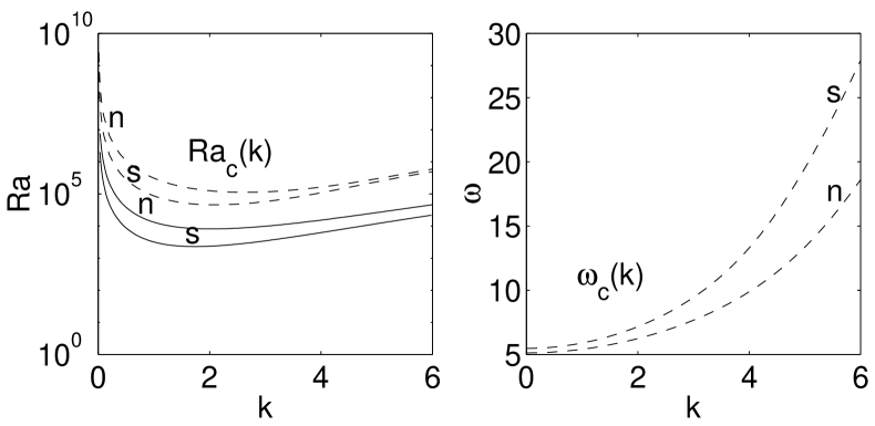
Figure 7: $\theta=0$. Viscous fluid; $\eta=0$, $\chi=1$; $\mu=1$, $Pr=6.7$, $Le=1$. In light of transformation (20), these results apply to $\theta=\pi$ as well. Curves of the marginal linear stability to 2D steady (the solid lines) and oscillatory (the dashed lines) disturbances, $Ra_{c}(k)$ and $\omega_{c}(k)$, for stress-free ($\bf{s}$) and no-slip ($\bf{n}$) slot boundary conditions. Notations $\bf{s}$ and $\bf{n}$ refer to the respective closest curves below them. (The analogue of the standing-wave oscillatory instabilities described in this figure is not reported for the inclined slot with viscous fluid considered herein below. It is then preceded by two types of 2D traveling-wave instability, one of which is related to the steady instabilities described in this figure.)

Oscillatory linear instability in a vertical slot with viscous fluid is discussed in Sec. 4.1.2 below. The broken boundary conditions symmetry then results in only one traveling wave. Such a disturbance arises from differential gradient diffusion, whether due to the distinction boundary alone or to both the distinction and the inverse boundaries. The direction of propagation of such a traveling wave matches the sign of the background contribution to the density (Fig. 1) at a sidewall with different boundary conditions from a (component) variable whose flux is prescribed there by (6)—(8). [This also applies both to the single traveling wave for $\eta=0$ and $\chi=1$ and to either of the symmetrically counter-propagating waves for $\eta=1$ and $\chi=0$ (Fig. 7 of [32]).] For the configuration in Fig. 1 ($\theta=\pi/2$), such a traveling wave has $+k_{y}$ in (11).

Growth of the disturbance with $-k_{y}$ in (11) is inconsistent with the effect of differential gradient diffusion combined with the along-slot gravity component. 2D instability to the standing-wave disturbance at $\theta=0$ cannot thus transform into the respective instability to the $e^{i(\omega\tau-k_{y}y)}$-mode traveling wave when $\theta$ is increased from $0$. As a consequence, instability to the latter traveling wave was found to vanish precipitously when $\theta$ increases from $0$ for all types of the boundary conditions.

The vanishing 2D instability is then replaced by the respective instability to 3D perturbations, since the latter perturbations are less sensitive to the above asymmetry introduced by the along-slot gravity component. (In particular, the along-slot gravity does not affect a perturbation with $k_{y}=0$ and $k_{z}\neq 0$.) Largely driven by the across-slot gravity, such a 3D instability also has to vanish as $\theta$ increases further. In view of these considerations, it is only the $e^{i(\omega\tau+k_{y}y+k_{z}z)}$-mode instability that is discussed herein below both for inviscid and for viscous fluid.

For any type of the boundary conditions, the inviscid $e^{i(\omega\tau+k_{y}y+k_{z}z)}$-mode instability with certain $k_{z}\geq 0$ possesses intervals of $k_{y}$ for which $Ra_{c}(k_{y})=\omega_{c}(k_{y})=0$ at some $\theta\in(0,\pi/2]$, as discussed below. Such a zero $\omega_{c}$, however, does not necessarily mean that the instability is steady. In particular, steady instabilities with finite $Ra_{c}$ are absent in viscous fluid for $\theta\in(0,\pi)$ and the boundary conditions considered herein. The zero-$\omega_{c}$ instability arising say at $\theta=\pi/2$ from the inviscid equations for oscillatory marginally unstable perturbation then has no immediate connection with the instability of a steady origin. It seems thus reasonable to expect that the perturbation developing at any small $Ra(k_{y})>0$ for some $\theta\in(0,\pi/2]$ and $k_{z}\geq 0$ would generally have a small $\omega(k_{y})>0$ as well. This is what is implied below, although such an effect of along-slot gravity is referred to as direct.

3.2.2 $\eta=\chi=0$

At $\theta=\pi/2$, the (2D) $e^{i(\omega\tau+k_{y}y)}$-mode instability would generally have to be manifested in the form of traveling cells whose sense of rotation is constant in time. In inviscid fluid, such a manifestation also has to take place at any $Ra>0$. In the absence of dissipation, even an infinitesimal horizontal density difference resulting from differential gradient diffusion could drive the perturbation. Eq. (17) then implies that such instability with $Ra_{c}(k_{y})=0$ also has to have $\omega_{c}(k_{y})=0$. For $\theta\in(0,\pi/2)$, however, the effect of across-slot gravity opposes amplitude growth of the perturbation cells whose sense of rotation does not change (Sec. 3.1.1).

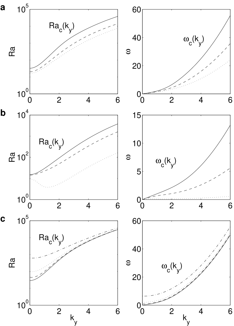
Figure 3: Inviscid fluid; $\eta=\chi=0$. Curves of the marginal linear stability to 3D ($k_{z}\geq 0$) oscillatory disturbances for different $k_{z}$, $Ra_{c}(k_{y})$ and $\omega_{c}(k_{y})$; $\mu=1$, $Le=1$. (a) $k_{z}=0$, the solid lines: $\theta=0$, the dashed lines: $\theta=\pi/8$, the dotted lines: $\theta=\pi/4$; (b) $k_{z}=0$, the solid lines: $\theta=3\pi/8$, the dashed lines: $\theta=0.9\pi/2$, the doted lines: $\theta=0.99\pi/2$; (c) $\theta=0.05\pi/2$, the solid lines: $k_{z}=0$, the dashed lines: $k_{z}=0.5$, the dotted lines: $k_{z}=1$, the dash-dot lines: $k_{z}=2$.

The combination of the effects of across-slot and along-slot gravity thus results in a decrease of $\omega_{c}(k_{y})$ with $\theta$ increasing from $0$ to $\pi/2$ [Fig. 3(a) and (b)]. This allows part of the rotation energy of a perturbation cell to come from the energy directly contributed by the along-slot gravity component in the current cycle of rotation. In the end of a cell rotation cycle, the whole rotation energy is transformed into the potential energy of perturbation stratification due to the across-slot gravity component. This potential energy is released in the next rotation cycle. As $\theta$ grows from $0$, the $Ra_{c}(k_{y})$ thus also decrease.

At the longest 2D wavelengths for $\eta=\chi=0$, the across-slot gravity component acts most effectively in opposing the direct contribution of the along-slot component to the rotation-energy increase. On the other hand, the shortest scales are least effective in accommodating the contribution of the along-slot gravity. It is thus a set of intermediate 2D wavelengths that becomes most unstable when $\theta=\pi/2$ is approached [Fig. 3(b)]. Decreasing for all $k_{y}$ as $\theta\rightarrow\pi/2$, such $Ra_{c}(k_{y})$ and $\omega_{c}(k_{y})$ also become identically zero at $\theta=\pi/2$.

Upon introduction of the long-wavelength expansion used above [32] into Eqs. (17) and (18) with $k=k_{y}$, the $k_{y}^{1}$ order of the $e^{i(\omega\tau+k_{y}y)}$-version of these equations and boundary conditions (15), (16), and (19) ($\eta=\chi=0$) yields

$$Ra_{c}(0)=24\omega_{0}^{2}/(2\cos\theta+\omega_{0}\sin\theta),$$ (29)

which is consistent with Eq. (26) for $\theta=0$. The values of $Ra_{c}(0)$ and $\omega^{c}_{k}(0)=\omega_{0}$ estimated from the numerical data underlying the (2D) marginal-stability curves in Fig. 3(a) and (b) [as well as from such data for $k_{y}<0$ (for which $\omega_{0}<0$ as well) not reported herein] were found to be fairly consistent with Eq. (29).

3.2.3 $\eta=\chi=1$

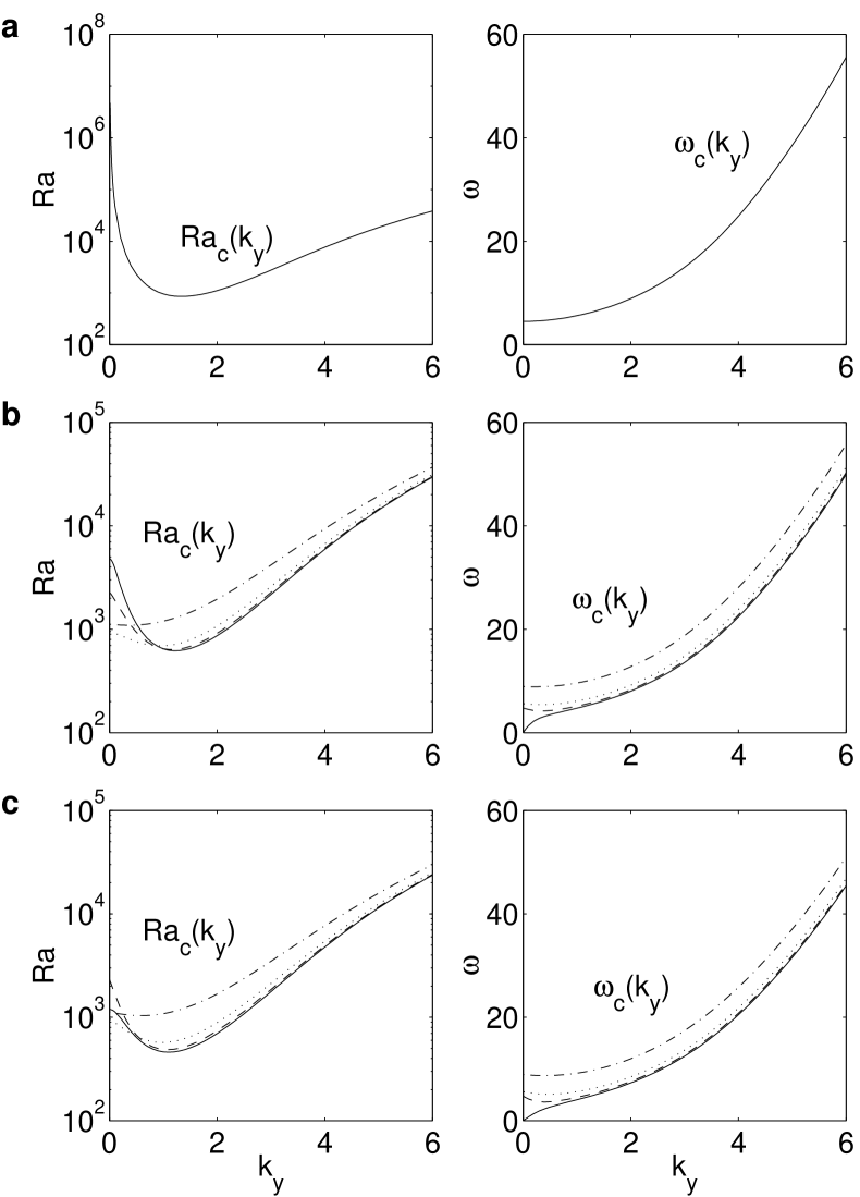
Figure 4: Inviscid fluid; $\eta=\chi=1$. Curves of the marginal linear stability to 3D ($k_{z}\geq 0$) oscillatory disturbances for different $k_{z}$, $Ra_{c}(k_{y})$ and $\omega_{c}(k_{y})$; $\mu=1$, $Le=1$. For (a)—(e), the solid lines: $k_{z}=0$, the dashed lines: $k_{z}=0.5$, the dotted lines: $k_{z}=1$, the dash-dot lines: $k_{z}=2$. (a) $\theta=0$; (b) $\theta=0.05\pi/2$; (c) $\theta=0.1\pi/2$; (d) $\theta=0.15\pi/2$; (e) $\theta=\pi/8$; (f) $k_{z}=0$, the solid lines: $\theta=\pi/4$, the dashed lines: $\theta=3\pi/8$, the dotted lines: $\theta=0.9\pi/2$, the dash-dot lines: $\theta=0.99\pi/2$.

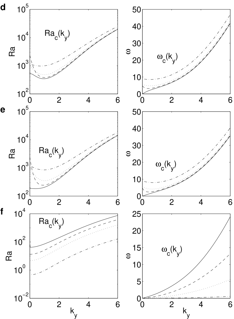
Figure 4: Inviscid fluid; $\eta=\chi=1$. Curves of the marginal linear stability to 3D ($k_{z}\geq 0$) oscillatory disturbances for different $k_{z}$, $Ra_{c}(k_{y})$ and $\omega_{c}(k_{y})$; $\mu=1$, $Le=1$. For (a)—(e), the solid lines: $k_{z}=0$, the dashed lines: $k_{z}=0.5$, the dotted lines: $k_{z}=1$, the dash-dot lines: $k_{z}=2$. (a) $\theta=0$; (b) $\theta=0.05\pi/2$; (c) $\theta=0.1\pi/2$; (d) $\theta=0.15\pi/2$; (e) $\theta=\pi/8$; (f) $k_{z}=0$, the solid lines: $\theta=\pi/4$, the dashed lines: $\theta=3\pi/8$, the dotted lines: $\theta=0.9\pi/2$, the dash-dot lines: $\theta=0.99\pi/2$.

At $\theta=\pi/2$ for $\eta=\chi=1$, the inviscid $e^{i(\omega\tau+k_{y}y)}$-mode instability also has to arise at any $Ra(k_{y})>0$, and thus $\omega_{c}(k_{y})=0$ for such instability as well. When only the across-slot gravity component is present ($\theta=0$), the vicinity of zero wave number is most stable to the disturbances that change their sense of rotation periodically in time [Fig. 4(a)]. It is therefore this region of $k_{y}$ that least opposes the direct contribution of along-slot gravity to the cell rotation energy. As $\theta$ increases from $0$, 2D $Ra_{c}(k_{y})$ thus decreases most significantly near $k_{y}=0$ [Fig. 4(a)—(e)]. Closer to $\theta=\pi/2$, however, the $Ra_{c}(k_{y})$ decreases noticeably and tends to $0$ as $\theta\rightarrow\pi/2$ for all $k_{y}$ [Fig. 4(f)].

As discussed in [32], three-dimensionality of most unstable disturbances could be a consequence of two general mathematical conditions. One of them (condition I) is dependence of $Ra_{c}$ only on wave number modulus $k$, as in

$$Ra_{c}(k_{y},k_{z})=Ra_{c}[(k^{2}_{y}+k^{2}_{z})^{1/2},0],$$ (30)

at a single value of some parameter ($\theta=0$ in this case) in whose vicinity $Ra_{c}$ depends on both components of $\vec{k}$. The other condition (condition II) is the existence of an interval where $Ra_{c}(k)$ is growing with decreasing $k$ at this value of the parameter. Three-dimensionality of the instability in a vicinity of the above parameter value then follows from the assumption that these conditions would largely apply at nearby values of such a parameter as well.

As discussed in Sec. 3.1.2 above, condition II holds at $\theta=0$ [Fig. 4(a)] near $k=0$ due to solute diffusion at the similarity boundary. This process is therefore responsible for the three-dimensionality of instability in Fig. 4(b) and (c). With the $Ra_{c}(k_{y})_{|\theta=\pi/2}=0$, the fast decrease of 2D $Ra_{c}(k_{y})$ near $k_{y}=0$ with $\theta$ growing from $0$ prevents such 3D disturbances from being dominant for the larger $\theta$. That no 3D most unstable disturbances are found in Fig. 3(c) is thus a consequence both of condition II being then not met for $\theta=0$ [Fig. 3(a)] and of the absence of another mechanism for 3D instability.

3.2.4 2D disturbances for $\eta=0$ and $\chi=1$

General.

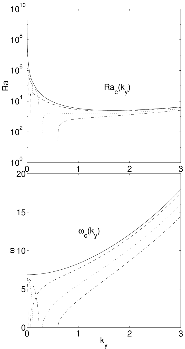
Figure 5: Inviscid fluid; $\eta=0$, $\chi=1$. Curves of the marginal linear stability to 2D ($k_{z}=0$) oscillatory disturbances, $Ra_{c}(k_{y})$ and $\omega_{c}(k_{y})$; $\mu=1$, $Le=1$. The nearly vertical curves of $Ra_{c}(k_{y})$ are expected to go to $Ra_{c}(k_{y})=0$. The solid lines: $\theta=(1\mp 1)\pi/2$, the dashed lines: $\theta=(1\mp 0.99)\pi/2$, the dotted lines: $\theta=(1\mp 0.95)\pi/2$, the dash-dot lines: $\theta=(1\mp 0.9)\pi/2$. The two values of $\theta$ are relevant in light of transformation (20).

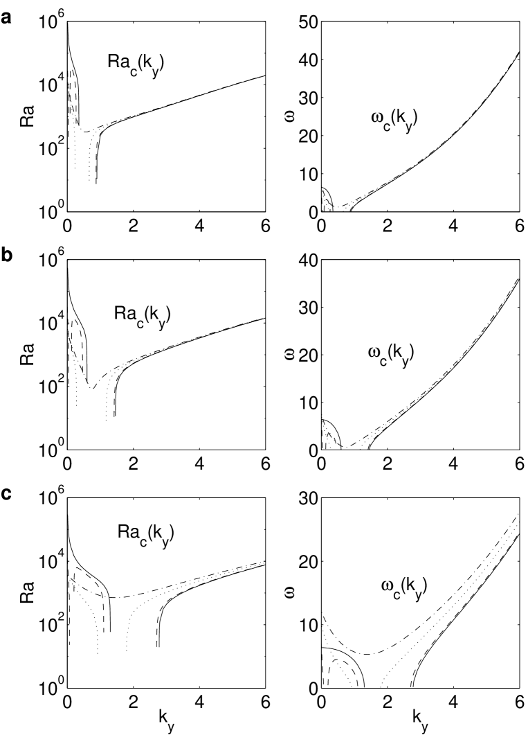
Figure 6: Inviscid fluid; $\eta=0$, $\chi=1$. Curves of the marginal linear stability to 3D ($k_{z}\geq 0$) oscillatory disturbances for different $k_{z}$, $Ra_{c}(k_{y})$ and $\omega_{c}(k_{y})$; $\mu=1$, $Le=1$. The nearly vertical curves of $Ra_{c}(k_{y})$ are expected to go to $Ra_{c}(k_{y})=0$. (a) $\theta=(1\mp 0.85)\pi/2$; (b) $\theta=(1\mp 0.75)\pi/2$; (c) $\theta=(1\mp 0.5)\pi/2$; (d) $\theta=(1\mp 0.25)\pi/2$; (e) $\theta=(1\mp 0.1)\pi/2$; (f) $\theta=\pi/2$. The two values of $\theta$ in (a)—(e) are relevant in light of transformation (20). The solid lines: $k_{z}=0$; the dashed lines: (a) $k_{z}=0.15$, (b) $k_{z}=0.25$, (c) $k_{z}=0.5$, (d) $k_{z}=1.3$, (e) $k_{z}=1.9$, (f) $k_{z}=1$; the dotted lines: (a) $k_{z}=0.4$, (b) $k_{z}=0.6$, (c) $k_{z}=1.5$, (d) $k_{z}=2.2$, (e) $k_{z}=3$, (f) $k_{z}=1.5$; the dash-dot lines: (a) $k_{z}=0.5$, (b) $k_{z}=0.77$, (c) $k_{z}=2$, (d) $k_{z}=2.8$, (e) $k_{z}=4.2$, (f) $k_{z}=2$. Additional data are provided in Table 1.

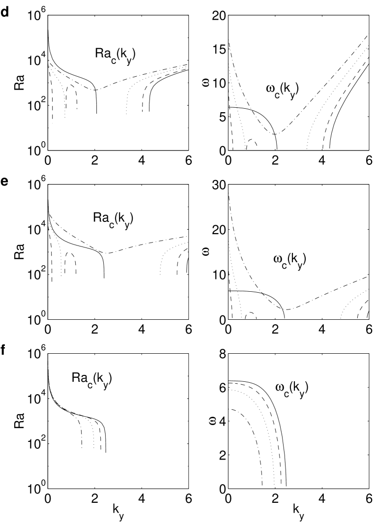
Figure 6: Inviscid fluid; $\eta=0$, $\chi=1$. Curves of the marginal linear stability to 3D ($k_{z}\geq 0$) oscillatory disturbances for different $k_{z}$, $Ra_{c}(k_{y})$ and $\omega_{c}(k_{y})$; $\mu=1$, $Le=1$. The nearly vertical curves of $Ra_{c}(k_{y})$ are expected to go to $Ra_{c}(k_{y})=0$. (a) $\theta=(1\mp 0.85)\pi/2$; (b) $\theta=(1\mp 0.75)\pi/2$; (c) $\theta=(1\mp 0.5)\pi/2$; (d) $\theta=(1\mp 0.25)\pi/2$; (e) $\theta=(1\mp 0.1)\pi/2$; (f) $\theta=\pi/2$. The two values of $\theta$ in (a)—(e) are relevant in light of transformation (20). The solid lines: $k_{z}=0$; the dashed lines: (a) $k_{z}=0.15$, (b) $k_{z}=0.25$, (c) $k_{z}=0.5$, (d) $k_{z}=1.3$, (e) $k_{z}=1.9$, (f) $k_{z}=1$; the dotted lines: (a) $k_{z}=0.4$, (b) $k_{z}=0.6$, (c) $k_{z}=1.5$, (d) $k_{z}=2.2$, (e) $k_{z}=3$, (f) $k_{z}=1.5$; the dash-dot lines: (a) $k_{z}=0.5$, (b) $k_{z}=0.77$, (c) $k_{z}=2$, (d) $k_{z}=2.8$, (e) $k_{z}=4.2$, (f) $k_{z}=2$. Additional data are provided in Table 1.

Transformation (20) makes the results of this Sec. 3.2.4 also applicable to $\theta\in[\pi/2,\pi]$. Assuming (20), they are however discussed below only in terms of $\theta\in[0,\pi/2]$. As seen from Fig. 5, any small increase of $\theta$ from $0$ leads to abrupt changes in the 2D marginal-stability curve for $\eta=0$ and $\chi=1$. These changes are associated with emergence of an interval of $k_{y}$ for which $Ra_{c}(k_{y})=\omega_{c}(k_{y})=0$. Such interval is born with its width and the lower limit tending to zero as $\theta\rightarrow 0$. Both these parameters of the interval then become finite when $\theta$ increases from $0$. They also continue to grow with $\theta$ increasing further (see the solid lines in Fig. 6).

In viscous fluid, steady instability for $\theta=0$ arises at finite viscous $Ra_{c}(k)$ (Fig. 7). (It precedes the respective instability to standing wave.) The inviscid steady $Ra_{c}(k)$ are then zero for all $k>0$ [Eq. (23) for $\theta=0$]. As discussed below (Sec. 4.1.3), however, such 2D steady viscous instability transforms into an oscillatory instability to traveling wave when $\theta$ is increased from $0$. As $\theta>0$, therefore, the argument just used does not apply. For $\theta>0$, the inviscid 2D instability with $Ra_{c}(k_{y})=\omega_{c}(k_{y})=0$ still ought to arise from the type of perturbation that is dominant at $\theta=\pi/2$, where the largest zero-threshold interval forms [Fig. 6(f)]. Generally, this has to be a traveling wave (whose speed turns infinitesimal with $\omega_{c}=0$). Such a perturbation is also the first to become unstable in viscous fluid for $\theta\in(0,\pi/2]$. Its manifestation would be most convenient to analyze in the presence of along-slot gravity alone.

Effect of the along-slot gravity.

In the presence of along-slot gravity alone [Fig. 6(f) for $k_{z}=0$], $Ra_{c}(k_{y})=\omega_{c}(k_{y})=0$ for $k_{y}>k_{y}^{2l}(0)\approx 2.4677$ (Table 1 for $\theta=\pi/2$ and $k_{z}=0$). Just below this value of $k_{y}$, however, both $Ra_{c}(k_{y})$ and $\omega_{c}(k_{y})$ abruptly increase to finite magnitudes. Additional calculations for $k_{y}>6$ and $\theta=\pi/2$ also suggest that the upper limit of the interval with zero $Ra_{c}(k_{y})$ and $\omega_{c}(k_{y})$ is at infinity.

As discussed below for viscous fluid (Sec. 4.1.2), differential gradient diffusion for $\eta=0$ and $\chi=1$ acts in concert at the vertical-slot boundaries. It gives rise to horizontal density differences that favor growth of the $e^{i(\omega\tau+k_{y}y)}$-mode traveling wave. In particular, the density perturbation generated around a clockwise-(counterclockwise-)rotating cell is largely specified by negative (positive) solute perturbation at the distinction boundary and temperature perturbation at the inverse boundary. This intensifies such downwards-propagating small-amplitude convective cells with a steady sense of rotation.

In the absence of dissipation, the horizontal density differences just described would give rise to the instability even when they are infinitesimal. Such an inviscid vertical-slot instability can thus arise for any $Ra>0$ no matter how much the effect of differential gradient diffusion diminishes with decreasing the wavelength. This is seen in Fig. 6(f) ($k_{z}=0$) for $k_{y}>k_{y}^{2l}(0)\approx 2.4677$.

For $\eta=0$ and $\chi=1$, however, either component forms a diffusion gradient at one of the boundaries. Such a diffusion is also the more effective the longer the wavelength is. When the wavelength exceeds a critical magnitude, therefore, the perturbation of either component could be neutralized by its diffusion at one of the boundaries. The infinitesimal horizontal density differences arising just above $Ra_{c}(k_{y})=\omega_{c}(k_{y})=0$ are thus eliminated by the component diffusion. Both $Ra_{c}(k_{y})$ and $\omega_{c}(k_{y})$ must then increase from zero as $k_{y}$ decreases below the critical value [$k_{y}=k_{y}^{2l}(0)\approx 2.4677$]. This increase is precipitous since such growing $\omega_{c}(k_{y})$ also lowers the efficiency of differential gradient diffusion, due to inconsistency between the $\omega_{c}(k_{y})$ and the increasing wavelength.

Combined effects of the along-slot and across-slot gravity.

The oscillatory instability for $\theta=0$ arises only at finite $Ra_{c}(k_{y})$ (Fig. 5). It is characterized by a standing wave, i.e. by convective cells whose sense of rotation changes periodically in time. Development of such a perturbation is inconsistent with that of a traveling wave arising due to the along-slot gravity, for such traveling-wave convective cells do not change their sense of rotation. For $\theta\in(0,\pi/2)$, the latter perturbation is also favored and opposed by the effects of across-slot gravity at the inverse and distinction boundaries, respectively, particularly when it is manifested with $Ra_{c}(k_{y})=\omega_{c}(k_{y})=0$. The steadily rotating cells would thus have to be localized near the inverse boundary to the extent $\theta$ is close to $0$.

Due to the expansion of the (steadily rotating) convective cells towards the distinction boundary with $\theta$ growing from $0$ to $\pi/2$, however, an opposition at this boundary to the steady sense of cell rotation is generally relevant for any $\theta<\pi/2$. Its relative role in rotation of a convective cell depends on the instability wavelength. As such wavelength decreases, in particular, the effect of across-slot gravity at the distinction boundary (opposing the steady sense of cell rotation) becomes relatively more pronounced with respect to that at the inverse boundary (favoring the steadily rotating cells). In addition, the shorter the wavelength the smaller the relative portion of streamline particles with across-slot density differences compared to that with such along-slot differences. The decreasing (increasing) wavelength thus also enhances (reduces) the effect of across-slot gravity with respect to that of along-slot gravity.

The minimal wavelength above which the zero-threshold steadily rotating cells are dominant then depends on $\theta$. Increasing from $0$ with $\theta$ decreasing from $\pi/2$ [Fig. 6 for $k_{z}=0$], it tends to infinity as $\theta\rightarrow 0$ (Fig. 5). Just above such a critical $k_{y}$[$\equiv k_{y}^{2u}(0)$ (Table 1 for $k_{z}=0$)] for $\theta\in(0,\pi/2)$, the steadily rotating perturbation cells fail to grow at infinitesimal $Ra$. The $Ra_{c}(k_{y})$ and $\omega_{c}(k_{y})$ thus increase from $0$.

As such $Ra_{c}(k_{y})$ and $\omega_{c}(k_{y})$ grow from $0$, however, the effect of across-slot gravity becomes increasingly more relevant. The efficiency of differential gradient diffusion for the steadily rotating perturbation cells then decreases. The $Ra_{c}(k_{y})$ and $\omega_{c}(k_{y})$ thus grow precipitously to such $k_{y}$. Relatively localized near the inverse boundary (to the extent $\theta$ is close to $0$), the steadily rotating convective cells then also transform into such perturbation cells as are relatively localized near the distinction boundary and change their sense of rotation with an adequate frequency. Control over the instability disturbances is thus largely transferred to the across-slot gravity component, whose action still remains affected by the direct contribution from the along-slot component.

When $\theta=\pi/2$ and $k_{y}<k_{y}^{2l}(0)_{|\theta=\pi/2}\approx 2.4677$, an infinitesimally small $Ra(k_{y})$ is neutralized by diffusion and thus fails to generate the instability. This takes place when such a diffusion process is equally active at both boundaries, as is expected at $\theta=\pi/2$. The closer $\theta$ is to $0$, however, the more localized the steadily rotating perturbation cells are near the inverse boundary. Compared to $\theta=\pi/2$, the overall effect of diffusion for such cells when $\theta\in(0,\pi/2)$ thus becomes asymmetrically divided between the components. Temperature diffusion at the distinction boundary is then less active than solute diffusion at the inverse boundary. For this reason, $k_{y}^{2l}(0)$ [below which the $Ra_{c}(k_{y})$ abruptly increases from $0$] also decreases with $\theta\in(0,\pi/2)$, from $k_{y}^{2l}(0)_{|\theta=\pi/2}\approx 2.4677$ to $0$ as $\theta\rightarrow 0$ (Fig. 5 and Fig. 6 for $k_{z}=0$).

3.2.5 3D disturbances for $\eta=0$ and $\chi=1$

General.

Although transformation (20) makes the results of this Sec. 3.2.5 also applicable to $\theta\in[\pi/2,\pi]$, except for Sec. 3.2.5, they are discussed below only in terms of $\theta\in[0,\pi/2]$. For any $\theta\in(0,\pi/2)$ in Table 1 and Fig. 6, the 3D lower and upper limits of the above zero-threshold interval of $k_{y}$, $k_{y}^{2l}(k_{z})$ and $k_{y}^{2u}(k_{z})$, decrease from $k_{y}^{2l0}\equiv k_{y}^{2l}(0)$ and $k_{y}^{2u0}\equiv k_{y}^{2u}(0)$, respectively, with $k_{z}$ increasing from $0$. They also continue to decrease with $k_{z}$ increasing further. For $\theta=\pi/2$, this formally applies only to $k_{y}^{2l}(k_{z})$, since $k_{y}^{2u}(k_{z})$ is then at infinity for any finite $k_{z}\geq 0$. In addition, another zero-threshold area arises from the vicinity of $k_{y}=0$ when $k_{z}>0$ [see the dashed lines in Fig. 6(a)—(e)]. However, the lower and upper limits of the latter area, $k_{y}^{3l}(k_{z})$ and $k_{y}^{3u}(k_{z})$, respectively, increase with growing $k_{z}$ (Table 1, $\theta\neq\pi/2$).

At a certain $k_{z}>0$, the interval of finite $Ra_{c}(k_{y})$ and $\omega_{c}(k_{y})$ between $k_{y}^{3u}(k_{z})$ and $k_{y}^{2l}(k_{z})$ thus vanishes, due to these parameters of $k_{y}$ merging with each other. A single continuous interval of zero $Ra_{c}(k_{y})$ and $\omega_{c}(k_{y})$ is then formed [the dotted lines in Fig. 6(a)—(e)]. Eventually, such a continuous interval also vanishes when $k_{y}^{3l}(k_{z})$ and $k_{y}^{2u}(k_{z})$ merge at a still larger $k_{z}$, leaving only nonzero $Ra_{c}$ and $\omega_{c}$ [the dash-dot lines in Fig. 6(a)—(e)]. Quantitative details of the behavior just described are reported in Table 1.

When 3D perturbations in Fig. 6 are dominant, their behavior cannot be explained only in the framework of the scenario emphasized in Sec. 3.2.3 above. Other mechanisms causing such a three-dimensionality would thus also have to exist. These mechanisms are associated with the nature of the 2D interval with $Ra_{c}(k_{y})=\omega_{c}(k_{y})=0$ discussed in Sec. 3.2.4 above.

$k_{y}^{2l}(k_{z})$ and $k_{y}^{2u}(k_{z})$.

For a given $\theta\in(0,\pi/2)$ and $k_{z}=0$, the 2D $Ra_{c}(k_{y})$ and $\omega_{c}(k_{y})$ increase from zero either when $k_{y}$ decreases below $k_{y}^{2l0}$ or when it increases above $k_{y}^{2u0}$. This takes place because for the respective wavelength intervals ($\lambda_{y}>2\pi/k_{y}^{2l0}$ and $\lambda_{y}<2\pi/k_{y}^{2u0}$) at the fixed $\theta\in(0,\pi/2)$, the perturbation cells with a steady sense of rotation cannot be destabilized by the effects of differential gradient diffusion at infinitesimal $Ra$ (see Sec. 3.2.4 above). Depending on the relative roles of the along-slot and across-slot gravity components, $k_{y}^{2l0}$ and $k_{y}^{2u0}$ are also the closer to $0$ the closer $\theta$ is to $0$.

Independent of the orientation of the axis of rotation of a convective cell, the effect of across-slot gravity does not change when $k_{z}$ increases from $0$. In this context, one could therefore refer to $k_{y}^{2l0}$ and $k_{y}^{2u0}$ as the respective critical values of $k$. With $k_{z}$ growing from $0$, however, the (relevant) projection of along-slot gravity on the axis orthogonal to the axis of cell rotation decreases.

Indeed, Eqs. (17) and (18) for $\vec{k}=(k_{y},k_{z})$ are identical to these equations for $\vec{k}=(k_{y},0)$ with that $\sin\theta$ in the latter is replaced by $(k_{y}/k)\sin\theta$ in the former. The relative role of along-slot gravity is thus diminished with respect to that in the 2D problem for $\vec{k}=(k_{y},0)$. This is similar to decreasing $\theta$ below the considered value. With increasing $k_{z}$, therefore, the actual values of $k_{y}^{2l}(k_{z})$ and $k_{y}^{2u}(k_{z})$ must be smaller than $q_{y}^{2l}(k_{z})\equiv[(k_{y}^{2l0})^{2}-k_{z}^{2}]^{1/2}$ and $q_{y}^{2u}(k_{z})\equiv[(k_{y}^{2u0})^{2}-k_{z}^{2}]^{1/2}$, respectively, as in Table 1 for any $\theta\neq\pi/2$.

For $\theta=\pi/2$, the relative role of the along-slot gravity component with respect to that of the (absent) across-slot component would remain infinite for any finite $k_{z}$. This has to lead to $k_{y}^{2l}(k_{z})=q_{y}^{2l}(k_{z})$, as is seen from Table 1 ($\theta=\pi/2$). In addition, the infinite value of $k_{y}^{2u0}$ is retained both by ${q_{y}^{2u}(k_{z})}_{|k_{z}>0}$ and by ${k_{y}^{2u}(k_{z})}_{|k_{z}>0}$ [Fig. 6(f) and Table 1 ($\theta=\pi/2$)].

For $\theta=\pi/2$, $k_{y}^{2l}(k_{z})$ and $k_{y}^{2u}(k_{z})$ should thus be exactly specified by $k_{y}^{2l0}$ and $k_{y}^{2u0}$($=\infty$). These latter have to serve as the critical values of $k$. Indeed, Eqs. (17) and (18) for $\theta=\pi/2$ suggest that

$$Ra_{c}(k_{y},k_{z})k_{y}/k=Ra_{c}(k,0).$$ (31)

This means that ${Ra_{c}(k_{y},k_{z})}_{|\theta=\pi/2}=0\Longleftrightarrow{Ra_{c}(k,0)}_{|\theta=\pi/2}=0$ for

$${k_{y}^{2l0}}_{|\theta=\pi/2}\leq(k_{y}^{2}+k_{z}^{2})^{1/2}\leq{k_{y}^{2u0}}_{|\theta=\pi/2}=\infty,$$ (32)

which is a condition for $k$[$=(k_{y}^{2}+k_{z}^{2})^{1/2}$] alone.

For $\theta=\pi/2$, 3D disturbances are thus most unstable at least for $k_{y}$ between ${q_{y}^{2l}(k_{z})}_{|\theta=\pi/2}$ ($<{k_{y}^{2l0}}_{|\theta=\pi/2}$) and ${k_{y}^{2l0}}_{|\theta=\pi/2}$. This could cause such a three-dimensionality for small $\pi/2-\theta$ as well. For any $\theta\in(0,\pi/2)$, however, $k_{y}^{2l}(k_{z})<q_{y}^{2l}(k_{z})$ (because $G=k_{y}/k<1$), as discussed above. The latter inequality is also an independent cause for dominance of 3D disturbances at $\theta\in(0,\pi/2)$. Additional causes of perturbation three-dimensionality for $\theta\in(0,\pi/2)$ are associated with another zero-threshold area in the $k_{y}$–$k_{z}$ plane. This area is described in Table 1 by $k_{y}^{3l}(k_{z})$ and $k_{y}^{3u}(k_{z})$.

General on $k_{y}^{3l}(k_{z})$ and $k_{y}^{3u}(k_{z})$.

The nature of the area with $Ra_{c}(k_{y},k_{z})=\omega_{c}(k_{y},k_{z})=0$ whose boundaries are described in Table 1 by $k_{y}^{3l}(k_{z})$ and $k_{y}^{3u}(k_{z})$ is fundamentally three-dimensional. First note that Eq. (30) is satisfied by $Ra_{c}(k_{y},k_{z})_{|\theta\in(0,\pi/2)}$ for $k_{y}=0$: ${Ra_{c}(0,k_{z})}_{|\theta\in(0,\pi/2)}={Ra_{c}(0,k)}_{|\theta\in(0,\pi/2)}={Ra_{c}(k,0)}_{|\theta=0}/\cos\theta$. In a vicinity of $k=0$ [Fig. 5], therefore, ${Ra_{c}(0,k)}_{|\theta\in(0,\pi/2)}$ decreases with increasing $k$. Conditions I and II discussed in Sec. 3.2.3 are then met. A region of small $k_{z}$ is thus expected to be dominated by 3D most unstable disturbances with small $G=k_{y}/k>0$. This observation, however, does not unravel the behavior of $k_{y}^{3l}(k_{z})$ and $k_{y}^{3u}(k_{z})$.

Eqs. (17) and (18) for $k_{y}>0$ also suggest that ${k_{y}^{3l}(k_{z})}_{|\theta=\theta_{3}}$ and ${k_{y}^{3u}(k_{z})}_{|\theta=\theta_{3}}$ specify such limits of the interval of $k$ over which $Ra_{c}(k,0)=\omega_{c}(k,0)=0$ for $\theta=\theta_{3}$ as are equal to the respective limits of two 2D intervals of $k_{y}$ over which $Ra_{c}(k_{y},0)=\omega_{c}(k_{y},0)=0$ for two smaller values of $\theta$. These are such respective $\theta=\theta_{2}$($<\theta_{3}$) as $\tan\theta_{2}=[k_{3y}(k_{z})/k_{3}(k_{z})]\tan\theta_{3}$, where $k_{3y}(k_{z})\equiv{k_{y}^{3l}(k_{z})}_{|\theta=\theta_{3}}$, ${k_{y}^{3u}(k_{z})}_{|\theta=\theta_{3}}$ and $k_{3}(k_{z})\equiv[{k^{2}_{3y}(k_{z})}+k_{z}^{2}]^{1/2}$. For any fixed $\theta\in(0,\pi/2)$, the increase of $G=k_{y}/k$ and $k_{z}$ from $0$ could thus give rise to a 3D area with $Ra_{c}(k_{y},k_{z})=\omega_{c}(k_{y},k_{z})=0$ analogously to the emergence of the 2D interval between $k_{y}^{2l0}$ and $k_{y}^{2u0}$ near $k_{y}=0$ when $\theta$ increases from $0$ (Fig. 5).

Three-dimensionality of the perturbation allows the relative effects of the two gravity components to be varied independently of $\theta$, and in particular to mimick the vicinity of $\theta=0$ at any $\theta\in(0,\pi/2)$. As parameters of $k_{y}$ between which $Ra_{c}(k_{y},k_{z})=\omega_{c}(k_{y},k_{z})=0$, $k_{y}^{3l}(k_{z})$ and $k_{y}^{3u}(k_{z})$ thus not only depend on the relation between the gravity components. They also specify this relation.

$k_{y}^{3l}(k_{z})$ and $k_{y}^{3u}(k_{z})$ for $k_{z}\rightarrow 0$.

For a fixed $\theta\in(0,\pi/2)$, the effects of across-slot and along-slot gravity are represented in Figs. 5 and 6(f), respectively. In view of Eq. (30), the dependence on $k_{y}$ for $k_{z}=0$ in Fig. 5 ($\theta=0$) also represents the dependence on $k$ for $k_{z}>0$. The dependence on $k_{z}>0$ in Fig. 6(f) is then given by Eq. (31). When $k\rightarrow 0$, $Re[d\tilde{u}(k,0)/dx]\asymp\omega_{c}(k,0)\asymp 1$ both at $\theta=0$ and at $\theta=\pi/2$ [as implied by the scaled continuity and Figs. 5 and 6(f)]. From Eqs. (17) and (18), the general solution for $\tilde{u}(x)$ then suggests that ${Ra_{c}(k,0)}_{|\theta=0}\asymp(1/k^{2})$ and ${Ra_{c}(k,0)}_{|\theta=\pi/2}\asymp(1/k)$ as $k\rightarrow 0$. Defining $R_{\theta_{1}}^{\theta_{2}}(k)\equiv{Ra_{c}(k,0)}_{|\theta=\theta_{2}}/{Ra_{c}(k,0)}_{|\theta=\theta_{1}}$, therefore, ${R_{0}^{\pi/2}(k)}_{|k\rightarrow 0}\asymp k$($\rightarrow 0$).

For $(k_{z}/k_{y})<\infty$ [$k_{z}=O(k_{y})$] when $k\rightarrow 0$, therefore, Eq. (31) implies that the effect of along-slot gravity dominates that of across-slot gravity. For a finite $\theta\in(0,\pi/2)$, this would be inconsistent with the existence of an infinitesimal area in the $k_{y}$–$k_{z}$ plane (for infinitesimal $k$) where $Ra_{c}(k_{y},k_{z})=\omega_{c}(k_{y},k_{z})=0$. Such an area could arise only when $\varepsilon\equiv(k_{y}/k_{z})\rightarrow 0$ [i.e., $k_{y}=o(k_{z})$] as well.

When $\varepsilon\rightarrow 0$ along with $k\rightarrow 0$ and $R_{c}(k)\equiv R_{0}^{\pi/2}(k)/k$, the necessary balance between the effects of the two gravity components [analogous to their 2D balance given by $0<(k_{y}/\tan\theta)<\infty$ as $k_{y}$($=k_{y}^{2u0}$) $\rightarrow 0$ and $\theta\rightarrow 0$],

$$0<\lim_{\stackrel{{\scriptstyle\scriptstyle{\varepsilon\rightarrow 0}}}{{\scriptstyle{k\rightarrow 0}}}}{[(k^{2}/k_{y})R_{0}^{\pi/2}(k)/k]}=\lim_{\stackrel{{\scriptstyle\scriptstyle{\varepsilon\rightarrow 0}}}{{\scriptstyle{k\rightarrow 0}}}}[R_{c}(k)(k^{2}/k_{y})]<\infty,$$ (33)

implies that $0<(k^{2}/k_{y})<\infty$ for $k\rightarrow 0$ and $\varepsilon\rightarrow 0$. In particular, numerical computations show that $R_{c}(k)$ is maximal at $k\rightarrow 0$ and that

$$\lim_{k\rightarrow 0}R_{c}(k)\approx 1.055.$$ (34)

Using the l’Hospital rule, one could then obtain, in particular,

$$(k^{2}/k_{y})\sim(k_{z}^{2}/k_{y})\sim k/\varepsilon\sim k_{z}/\varepsilon\sim 2k/(\frac{dk_{y}}{dk})\sim 2k_{z}/(\frac{dk_{y}}{dk_{z}})\sim$$

$$\frac{dk}{d\varepsilon}\sim\frac{dk_{z}}{d\varepsilon}\sim[\frac{d(k^{2})}{d(\varepsilon^{2})}]^{1/2}\sim[\frac{d(k_{z}^{2})}{d(\varepsilon^{2})}]^{1/2}\sim\frac{dk_{y}}{d(\varepsilon^{2})}\sim 1/[\frac{dk_{y}}{d(k^{2})}]\sim$$

$$1/[\frac{dk_{y}}{d(k_{z}^{2})}]\sim 2/(\frac{d^{2}k_{y}}{dk^{2}})\sim 2/(\frac{d^{2}k_{y}}{dk_{z}^{2}})\;\;\;\;(k\rightarrow 0,\;\;\varepsilon\rightarrow 0),$$ (35)

where $\sim$ denotes the asymptotic equivalence. With such necessary conditions, the relation between the effects of the two gravity components is similar to that in the 2D problem when $\theta\rightarrow 0$. For any finite $\theta\in(0,\pi/2)$, such infinitesimal $k_{y}^{3l}(k_{z})$[$=o(k_{z})$] and $k_{y}^{3u}(k_{z})$[$=o(k_{z})$] as maintain (35) could thus arise, $Ra_{c}(k_{y},k_{z})=\omega_{c}(k_{y},k_{z})=0$ for $k_{y}(k_{z})\in[k_{y}^{3l}(k_{z}),k_{y}^{3u}(k_{z})]$.

$k_{y}^{3l}(k_{z})$ and $k_{y}^{3u}(k_{z})$ for finite $k_{z}$.

Equivalence relations (35) imply that for $k_{y}=k_{3y}(k_{z})$[$\equiv k_{y}^{3l}(k_{z})$,$k_{y}^{3u}(k_{z})$], $dk_{y}/dk_{z}\rightarrow 0$ as $k_{z}\rightarrow 0$ and $\varepsilon\rightarrow 0$. $k_{3y}(k_{z})$ then has a local minimum in this limit, since $d^{2}k_{y}/dk_{z}^{2}>0$ as $k_{z}\rightarrow 0$ and $\varepsilon\rightarrow 0$ for such a $k_{y}(k_{z})$. One could thus expect that the respective $dk_{y}/dk_{z}$ be positive within a small (positive) vicinity of $k_{z}=0$. It is generally shown below that when $k_{y}=k_{3y}(k_{z})$, $dk_{y}/dk_{z}>0$ for any $k_{z}$($>0$).

As discussed in Sec. 3.2.4, $k_{y}^{2l0}$ and $k_{y}^{2u0}$ grow with increasing (decreasing) $\theta\in(0,\pi/2)$ [$\theta\in(\pi/2,\pi)$], when the along-slot gravity is enhanced with respect to the across-slot gravity. Eq. (17) also suggests that the variation of $G(k,k_{z})=(k^{2}-k_{z}^{2})^{1/2}/k$ causes qualitatively the same effect on the relation between the gravity components as that of $|\tan\theta|$. $k_{3}(k_{z})${$\equiv[k^{2}_{3y}(k_{z})+k_{z}^{2}]^{1/2}$} thus has to grow with $G$: $dG(k,k_{z})/dk>0$ for $k=k_{3}(k_{z})$. This yields

$$\frac{dk_{z}}{dk_{3}}<\frac{k_{z}}{k_{3}}\Longleftrightarrow\frac{dk_{3}}{dk_{z}}>\frac{k_{3}}{k_{z}}.$$ (36)

Since $\varepsilon\rightarrow 0$ as $k_{z}\rightarrow 0$ for $k_{y}=k_{3y}(k_{z})$, one could expect that $G(k_{3},k_{z})=k_{3y}/k_{3}$ [$\sim k_{y}/k_{z}=\varepsilon$ for infinitesimal $k_{z}$ and $k_{y}=k_{3y}(k_{z})=o(k_{z})$] would increase with $k_{z}$ within a small vicinity of $k_{z}=0$. Such a behavior is found to hold for any finite $k_{z}$($>0$) as well: (36) also implies that $dG(k,k_{z})/dk_{z}>0$ for $k=k_{3}(k_{z})$. With $G=k_{y}/(k_{y}^{2}+k_{z}^{2})^{1/2}$ and $k_{y}=k_{3y}(k_{z})$, however,

$$\frac{dG}{dk_{z}}=\frac{k_{z}^{2}}{k^{3}}(\frac{dk_{y}}{dk_{z}}-\varepsilon)>0.$$ (37)

This means that $dk_{3y}(k_{z})/dk_{z}>k_{3y}(k_{z})/k_{z}>0$.

$k_{y}^{3l}(k_{z})$ and $k_{y}^{3u}(k_{z})$ thus have to only increase with growing $k_{z}$. Such a behavior is consistent with the data in Table 1. Due to $k_{y}^{2l}(k_{z})$ and $k_{y}^{2u}(k_{z})$ decreasing with growing $k_{z}$, it also explains both the merging of $k_{y}^{3u}(k_{z})$ with $k_{y}^{2l}(k_{z})$ and that of $k_{y}^{3l}(k_{z})$ with $k_{y}^{2u}(k_{z})$.

Another aspect of the data in Table 1 is that for a fixed $k_{z}$, $k_{y}^{3l}(k_{z})$ and $k_{y}^{3u}(k_{z})$ are the closer to $0$ the closer $\theta$ is to $\pi/2$. This is associated with their ratio between the gravity components, their $G(k_{y},k_{z})\tan\theta$, being a function of $k$ alone, as suggested by Eq. (17). Such a function thus has to be proportional to $1/k$. For $k_{z}$($>0$) being fixed and $k_{y}=k_{3y}(k_{z},\theta)$, therefore, $d[k_{y}(k_{z},\theta)\tan\theta]/d\theta=0$ implies $\partial k_{y}(k_{z},\theta)/\partial\theta<0$ [$\partial k_{y}(k_{z},\theta)/\partial\theta>0$] for $\theta\in(0,\pi/2)$ [$\theta\in(\pi/2,\pi)$]:

$$\frac{\partial k_{y}(k_{z},\theta)}{\partial\theta}=-\frac{2}{\sin(2\theta)}k_{y}(k_{z},\theta).$$ (38)

Since $k_{y}^{2l}(k_{z})$ and $k_{y}^{2u}(k_{z})$ increase with $\theta$ approaching $\pi/2$, the ultimate vanishing of all areas with $Ra_{c}(k_{y},k_{z})=\omega_{c}(k_{y},k_{z})=0$, when $k_{y}^{3l}(k_{z})$ and $k_{y}^{2u}(k_{z})$ merge, takes place at the larger $k_{z}$ the closer $\theta$ is to $\pi/2$ (Table 1). For $\theta=\pi/2$, the absence of across-slot gravity makes the relation between the gravity components independent of $G$. Eq. (31) thus prohibits the existence of $k_{y}^{3l}(k_{z})\neq 0$ and $k_{y}^{3u}(k_{z})\neq 0$ for any $k_{z}$.

4 Viscous fluid

4.1 Small-amplitude oscillatory convection

4.1.1 $\theta=0$

Diffusion for $\eta=\chi$.

Despite dissipation, different component conditions at one boundary give rise to oscillatory instability at $\theta=0$ both for $\eta=\chi=0$ and for $\eta=\chi=1$. For the no-slip boundaries, this is illustrated in Fig. 8. As could be expected, $Ra_{c}(k)$ and $\omega_{c}(k)$ are higher for both values of $\eta=\chi$ [Fig. 8(a)] than for $\eta=1$ and $\chi=0$ [Fig. 5(a) in [32]]. Fig. 8(b) also exhibits decaying oscillations of $\delta Ra_{c}(k)\equiv{Ra_{c}(k)}_{|\eta=\chi=0}-{Ra_{c}(k)}_{|\eta=\chi=1}$ and $\delta\omega_{c}(k)\equiv{\omega_{c}(k)}_{|\eta=\chi=0}-{\omega_{c}(k)}_{|\eta=\chi=1}$.

The behavior of $\delta Ra_{c}(k)$ and $\delta\omega_{c}(k)$ in Fig. 8(b) arises from a more effective role of the distinction boundary for $\eta=\chi=1$. Compared to $\eta=\chi=0$, diffusion at the similarity boundary reduces the component perturbation scales for $\eta=\chi=1$ by the same fraction (that increases with the wavelength). Specified by the background scales, the gradient disparity at the distinction boundary then grows with respect to such a reduced component scale. The relative amplitude of convective motion thus also grows, generating a relatively larger gradient disparity for the next rotation cycle. With such more efficient mechanism, the small-$k$ instability for $\eta=\chi=1$ precedes that for $\eta=\chi=0$.

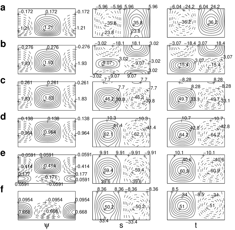
Figure 9: $\theta=0$. Viscous fluid and no-slip slot boundaries; $\eta=\chi=0$. Perturbation temporal behavior throughout a half of the oscillation period $\tau_{p}\approx 18\delta\tau$ ($\delta\tau=0.05$) just beyond the onset of 2D oscillatory instability. It was obtained from the numerical simulation of evolution of the linearized Eqs. (1)—(3) in response to the initial disturbance proportional to the background state after initial time $\tau_{i}\approx 340000$ has passed; $\lambda=2$, $\mu=1$, $Ra=87340$, $Pr=6.7$, $Le=1$. With this $\tau_{i}$, all perturbation modes other than the unstable mode ($\tau_{p}\approx 18\delta\tau$) are practically negligible. $\psi$: perturbation streamlines; $s$: isolines of solute concentration perturbation; $t$: perturbation isotherms. The actual relative values of the streamfunction perturbation are equal to $10^{-3}$ times the respective values in the figure. The solid and dashed streamlines designate the clockwise and counterclockwise rotation and are equally spaced within the positive and negative streamfunction intervals, respectively. The solid and dash-dot isolines of the component perturbations are equally spaced within the positive and negative component perturbation intervals, respectively. (a) $\tau=\tau_{i}+\delta\tau$; (b) $\tau=\tau_{i}+3\delta\tau$; (c) $\tau=\tau_{i}+5\delta\tau$; (d) $\tau=\tau_{i}+7\delta\tau$; (e) $\tau=\tau_{i}+8\delta\tau$; (f) $\tau=\tau_{i}+9\delta\tau$.

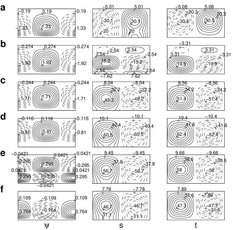
Figure 10: $\theta=0$. Viscous fluid and no-slip slot boundaries; $\eta=\chi=1$. Perturbation temporal behavior throughout a half of the oscillation period $\tau_{p}\approx 18\delta\tau$ ($\delta\tau=0.05$) just beyond the onset of 2D oscillatory instability. It was obtained from the numerical simulation of evolution of the linearized Eqs. (1)—(3) in response to the initial disturbance proportional to the background state after initial time $\tau_{i}\approx 120000$ has passed; $\lambda=2$, $\mu=1$, $Ra=85040$, $Pr=6.7$, $Le=1$. With this $\tau_{i}$, all perturbation modes other than the unstable mode ($\tau_{p}\approx 18\delta\tau$) are practically negligible. $\psi$: perturbation streamlines; $s$: isolines of solute concentration perturbation; $t$: perturbation isotherms. The actual relative values of the streamfunction perturbation are equal to $10^{-3}$ times the respective values in the figure. The solid and dashed streamlines designate the clockwise and counterclockwise rotation and are equally spaced within the positive and negative streamfunction intervals, respectively. The solid and dash-dot isolines of the component perturbations are equally spaced within the positive and negative component perturbation intervals, respectively. (a) $\tau=\tau_{i}+\delta\tau$; (b) $\tau=\tau_{i}+3\delta\tau$; (c) $\tau=\tau_{i}+5\delta\tau$; (d) $\tau=\tau_{i}+7\delta\tau$; (e) $\tau=\tau_{i}+8\delta\tau$; (f) $\tau=\tau_{i}+9\delta\tau$.

Figs. 9(a),(f) and 10(a),(f) illustrate the stage of potential energy release via differential gradient diffusion. The ratio of the streamfunction perturbation scale to that of either component for $\eta=\chi=1$ [Fig. 10(a) and (f)] exceeds this ratio for $\eta=\chi=0$ [Fig. 9(a) and (f)]. Thus relatively more intensive at $\eta=\chi=1$, such a convective motion gives rise to new component perturbation stratifications [Figs. 9(b)—(d) and 10(b)—(d)]. The latter arise from the respective background gradients with the ones for $\eta=\chi=1$ being smaller.

Via the higher gradient of temperature diffusion at the distinction boundary, the perturbation stratification thus formed opposes the current sense of cell rotation [Figs. 9(c),(d) and 10(c),(d)]. Due to the higher efficiency of such differential diffusion, this opposition is more pronounced for the fixed-value similarity boundary than for the flux one. With respect to the perturbation scale of either component, in particular, the streamfunction scale for $\eta=\chi=1$ [Fig. 10(c),(d)] becomes smaller than that for $\eta=\chi=0$ [Fig. 9(c),(d)]. The relatively unequal potential energies of perturbation stratification so generated are then utilized by the reversely rotating cells [Figs. 9(e),(f) and 10(e),(f)].

Diffusion and dissipation for $\eta=\chi$.

A consequence of differential gradient diffusion being more efficient for $\eta=\chi=1$ than for $\eta=\chi=0$ is thus a relatively larger variation of the respective velocity scale. For about the same variation time at a fixed wavelength, this implies steeper spatial velocity gradients for $\eta=\chi=1$ and thus the respectively greater dissipation.

Of two dissipation mechanisms affecting the instability [32], one is merely associated with damping all motions. Its overall effect is the greater the shorter the instability wavelength is. The other mechanism causes an efficiency reduction for the instability feedback. Such feedback links the component perturbation potential energy generated when a cell rotates in one sense and the intensity of rotation of such a cell in the opposite sense. The effect of this mechanism depends on the along-slot part of dissipation of a convective cell. It is the increasing role of the latter dissipation mechanism that causes $Ra_{c}(k)$ to rise infinitely with $k$ decreasing to $0$ for both $\eta=\chi$. The higher efficiency of differential gradient diffusion for $\eta=\chi=1$ thus becomes relevant for such $k$.

When the wavelength increases, the growing destabilizing contribution of diffusion at the similarity boundary is increasingly opposed by the respective enhancement of only the second of the two above dissipation mechanisms. Both these counter effects are commensurately augmented by the growing wavelength. The enhancement of overall dissipation for $\eta=\chi=1$ (with respect to $\eta=\chi=0$) would thus have to remain of a limited relative significance compared to the respectively higher efficiency of differential gradient diffusion.

For sufficiently long waves, therefore, it is the efficiency of differential gradient diffusion that specifies at which value of $\eta=\chi$ the instability sets in first: $\delta Ra_{c}(k)>0$ [Fig. 8(b)]. For a fixed wavelength, in addition, the optimal frequency with which the convective cells change their sense of rotation has to be largely specified by the background gradient of the stably stratified component. For $\mu=1$, therefore, $\delta\omega_{c}(k)>0$ for such $k$.

When the instability wavelength decreases, the effect of the first dissipation mechanism is enhanced, due to the across-slot motion being augmented. The role of the overall dissipation disparity between $\eta=\chi=1$ and $\eta=\chi=0$ then grows with respect to the (diminishing) effect of diffusion at the similarity boundary. $|\delta Ra_{c}(k)|$ and $|\delta\omega_{c}(k)|$ thus decay with increasing $k$ [Fig. 8(b)].

However, the dissipation enhancement for $\eta=\chi=1$ eventually dominates the respectively higher efficiency of differential diffusion underlying it. $\delta Ra_{c}(k)$ thus becomes negative [Fig. 8(b)], and then so does $\delta\omega_{c}(k)$. The overall efficiency of the combined effects of diffusion and dissipation then becomes higher for $\eta=\chi=0$. An additional dissipation arising above the $k$ where $\delta Ra_{c}(k)=0$ would therefore be greater for $\eta=\chi=0$ than for $\eta=\chi=1$. When the relative role of the disparity between such additional dissipations is augmented sufficiently with $k$ increasing further, the sign of $\delta Ra_{c}(k)$ changes again.

The oscillatory nature of decay of $\delta Ra_{c}(k)$ and $\delta\omega_{c}(k)$ in Fig. 8(b) is thus associated with the additional dissipation arising above a critical value of $k$ where $\delta Ra_{c}(k)=0$ acting against the increase of $|\delta Ra_{c}(k)|$. The value of $\eta=\chi$ at which the overall efficiency of diffusion and dissipation becomes higher above such a critical $k$ is also characterized by more dissipation.

The values of $k$ where $\delta\omega_{c}(k)=0$ in Fig. 8(b) slightly exceed the respective $k$ where $\delta Ra_{c}(k)=0$. A comparatively more time for diffusion and dissipation is thus provided for the value of $\eta=\chi$ that has just [when $\delta Ra_{c}(k)=0$] become a less efficient combination of these processes. Over a short interval of $k$, this outweighs the mismatch between the signs of $\delta\omega_{c}(k)$ and $\delta Ra_{c}(k)$.

Unreported herein, the values of $k$ at which $\delta Ra_{c}(k)$ and $\delta\omega_{c}(k)$ change sign for stress-free boundary conditions were found to be respectively smaller than those for the no-slip conditions. This could be associated with the higher no-slip $Ra_{c}(k)$ being more important for delaying the effects of dissipation than the decrease of (along-slot) dissipation due to the stress-free boundaries.

$\eta=0$ and $\chi=1$.

Oscillatory instability for $\eta=0$ and $\chi=1$ at $\theta=0$ ($\theta=\pi$) arises where the fluid is already unstable to steady disturbances (Fig. 7). It is however instructive to comment on its $Ra_{c}(k)$ and $\omega_{c}(k)$ compared to those for $\eta=\chi$. For $\eta=0$ and $\chi=1$, the oscillatory perturbation has to be localized near the distinction (inverse) boundary. With respect to $\eta=\chi$, this implies a higher efficiency of differential gradient diffusion at this boundary. The relative portion of moving fluid particles with the generated horizontal density differences is larger for $\eta=0$ and $\chi=1$ than for $\eta=\chi$.

For $\eta=0$ and $\chi=1$, however, differential gradient diffusion at the inverse (distinction) boundary opposes amplitude growth of a convective cell whose sense of rotation changes periodically. This opposition is dominant for relatively long wavelengths, whereas the higher efficiency of oscillatory across-slot motions is more important for the short waves. In viscous fluid, such a higher efficiency at the large $k$ for $\eta=0$ and $\chi=1$ is also expected to generate a relatively higher dissipation. This would however be offset by the across-slot cell path being shorter for $\eta=0$ and $\chi=1$ than for $\eta=\chi$. The effects of dissipation thus have to be relatively little important in the present context.

As $k$ exceeds a certain value, $Ra_{c}(k)$ for $\eta=0$ and $\chi=1$ thus changes from being larger to being smaller than that at either of $\eta=\chi$. For inviscid fluid and for viscous fluid with no-slip and stress-free boundary conditions, such a value is between $4.9$ and $5.3$. For $\omega_{c}(k)$, such a value is between $5.6$ and $5.8$. [The data for most such cases are depicted in Figs. 3(a) and 4(a), partly in Fig. 5, as well as in Figs. 7 and 8(a).] The larger critical values of $k$ for $\omega_{c}(k)$ further relatively diminish the effect of differential gradient diffusion at the inverse (distinction) boundary. Until then, this effect remains more important than the match between $\omega_{c}(k)$ and the respective stable solute stratification.

4.1.2 $\theta\in[0,\pi/2]$

General.

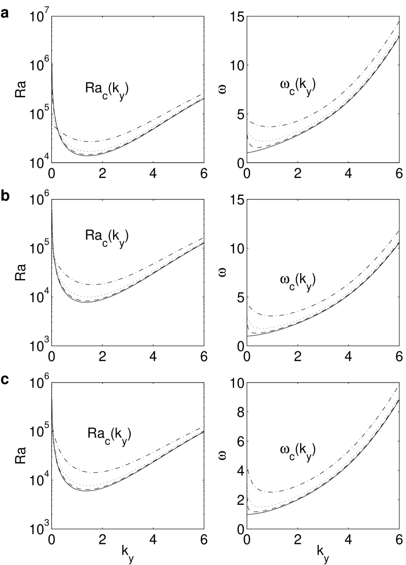
Figure 11: Viscous fluid and no-slip slot boundaries; $\eta=\chi=0$. Curves of the marginal linear stability to 3D ($k_{z}\geq 0$) oscillatory disturbances for different $k_{z}$, $Ra_{c}(k_{y})$ and $\omega_{c}(k_{y})$; $\mu=1$, $Pr=6.7$, $Le=1$. The solid lines: $k_{z}=0$, the dashed lines: $k_{z}=0.5$, the dotted lines: $k_{z}=1$, the dash-dot lines: $k_{z}=2$. (a) $\theta=0.25\pi/2$; (b) $\theta=0.5\pi/2$; (c) $\theta=0.75\pi/2$.

The marginal-stability curves in Fig. 8(a) meet conditions I and II emphasized in Sec. 3.2.3 above. Here condition II holds due to the second dissipation mechanism (Sec. 4.1.1) for both $\eta=\chi$ and also due to solute diffusion at the similarity boundary for $\eta=\chi=1$. 3D disturbances are thus the first to arise near $k_{y}=0$ for small $\theta>0$ [Figs. 11(a) and 12(a)]. Their dominance intervals of $k_{y}$ are shorter than those for $\eta=1$ and $\chi=0$ [32]. This results from a less favorable combination of the effects of two gravity components. The 2D instability for $\eta=1$ and $\chi=0$ sets in at $\theta=0$ before and at $\theta=\pi/2$ after those for $\eta=\chi$. In particular, the pattern of two counter-traveling waves for $\eta=1$ and $\chi=0$ at $\theta=\pi/2$ (Fig. 7 in [32]) generates more dissipation than such a single-wave pattern for $\eta=\chi$ considered below.

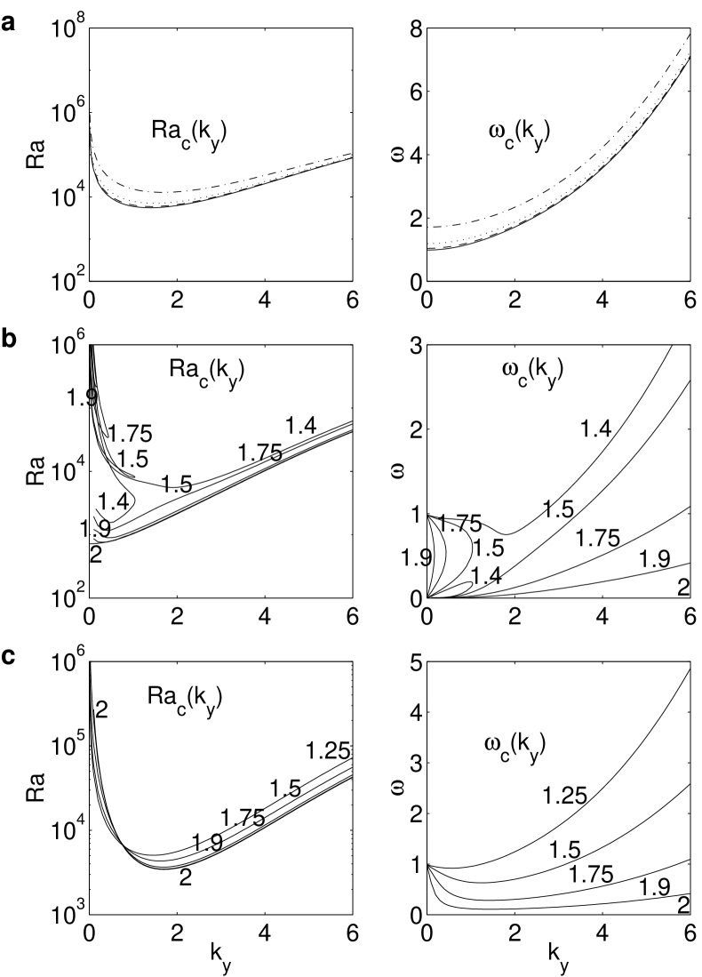
Figure 13: Viscous fluid and no-slip slot boundaries. Curves of the marginal linear stability to 3D ($k_{z}\geq 0$) oscillatory disturbances for different $k_{z}$, $Ra_{c}(k_{y})$ and $\omega_{c}(k_{y})$; $\mu=1$, $Pr=6.7$, $Le=1$. The solid lines: $k_{z}=0$, the dashed lines: $k_{z}=0.5$, the dotted lines: $k_{z}=1$, the dash-dot lines: $k_{z}=2$. (a) $\theta=\pi/2$, $\eta=\chi=0$ and $\eta=\chi=1$; (b) $\eta=\chi=0$; (c) $\eta=\chi=1$. In (b) and (c), $\theta=\vartheta\pi/2$, where the values of $\vartheta$ are given in these figures next to their respective closest curves the numbers do not intersect and for $\vartheta=2$, the instability is steady: $\omega_{c}(k_{y})=0$. For the lowest $\omega_{c}(k_{y})>0$ in (b) and for $\vartheta=2$ in (c), the data near $k_{y}=0$ (where such stable data were numerically difficult to obtain) are not presented. For such data, ${Ra_{c}(k_{y})}_{|k_{y}\rightarrow 0}\rightarrow\infty$ are assumed.

As for $\eta=1$ and $\chi=0$, however, the intervals of $k_{y}$ with 3D most unstable disturbances vanish for $\eta=\chi$ only when $\theta=\pi/2$ (Figs. 11 and 12). With $Re[d\tilde{u}(k)/dx]_{|\theta=0}\asymp{\omega_{c}(k)}_{|\theta=0}\asymp 1$ and $Re[d\tilde{u}(k,0)/dx]_{|\theta=\pi/2}\asymp{\omega_{c}(k,0)}_{|\theta=\pi/2}\asymp 1$ as $k\rightarrow 0$ [Figs. 8(a) and 13(a)], the general solution for $\tilde{u}(x)$ from Eqs. (12) and (13) suggests that (Sec. 3.2.5) $[R_{0}^{\pi/2}(k)/G]_{|k\rightarrow 0}\asymp(k/G)_{|k\rightarrow 0}>0\Longleftrightarrow G_{|k\rightarrow 0}=O(k)$($\rightarrow 0$). Arising from the across-slot gravity alone, the three-dimensionality is thus retained by a sufficiently small $G=k_{y}/k$ so long as $\theta<\pi/2$. It could also be viewed as coming from conditions I and II at $G=0$. As $k_{y}\rightarrow 0$ for a fixed $k_{z}>0$, in particular, the $Ra_{c}(k_{y},k_{z})\cos\theta$ and $\omega_{c}(k_{y},k_{z})$ tend to the respective 2D $Ra_{c}(k_{z})$ and $\omega_{c}(k_{z})$ at $\theta=0$ [Figs. 8(a), 11, and 12].

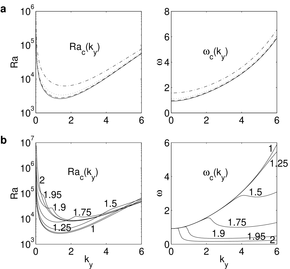
Figure 14: Viscous fluid and no-slip slot boundaries; $\eta=0$, $\chi=1$. Curves of the marginal linear stability to 3D ($k_{z}\geq 0$) oscillatory disturbances for different $k_{z}$, $Ra_{c}(k_{y})$ and $\omega_{c}(k_{y})$; $\mu=1$, $Pr=6.7$, $Le=1$. The solid lines: $k_{z}=0$, the dashed lines: $k_{z}=0.5$, the dotted lines: $k_{z}=1$, the dash-dot lines: $k_{z}=2$. (a) $\theta=\pi/2$; (b) $\theta=\vartheta\pi/2$ and $\theta=(2-\vartheta)\pi/2$, where the values of $\vartheta$ are given in the figure next to their respective closest curves the numbers do not intersect and for $\vartheta=2$, the instability is steady: $\omega_{c}(k_{y})=0$. The two values of $\theta$ in (b) are applicable in light of transformation (20). For $\vartheta=2$ in (b), the data near $k_{y}=0$ (where such stable data were numerically difficult to obtain) are not presented.

In view of transformation (20), $Ra_{c}(k_{y},k_{z})$ and $\omega_{c}(k_{y},k_{z})$ for $\eta=0$ and $\chi=1$ when $\theta\in[0,\pi/2)$ are addressed when $\theta\in(\pi/2,\pi]$ is considered in Sec. 4.1.3 below. Since Eq. (31) also applies to viscous fluid, the 2D disturbances must be most unstable at $\theta=\pi/2$ for any $\eta$ and $\chi$. This is seen from Figs. 13(a) and 14(a). The former figure is independent of $\eta=\chi$. The respective instability mechanisms for $\eta=\chi$ thus have to be such as are essentially due only to the distinction boundary. By virtue of Eq. (31), this could be discussed in the 2D framework alone. The mechanisms of 2D instability at $\theta=\pi/2$ for $\eta=\chi$ are thus considered below along with such a mechanism for $\eta=0$ and $\chi=1$.

2D instability mechanisms for $\theta=\pi/2$.

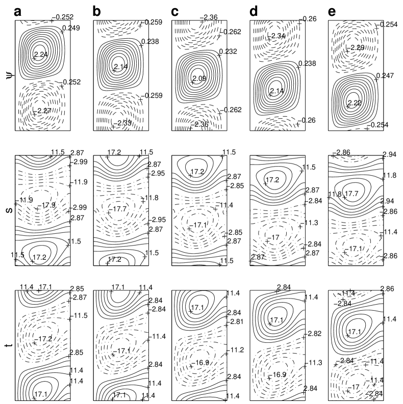
Figure 15: $\theta=\pi/2$. Viscous fluid and no-slip slot boundaries; $\eta=\chi=0$. Perturbation temporal behavior throughout nearly a half of the oscillation period $\tau_{p}\approx 46\delta\tau$ ($\delta\tau=0.05$) just beyond the onset of 2D oscillatory instability. It was obtained from the numerical simulation of evolution of the linearized Eqs. (1)—(3) in response to the initial disturbance proportional to the background state after initial time $\tau_{i}\approx 12000$ has passed; $\lambda=2$, $\mu=1$, $Ra=11292$, $Pr=6.7$, $Le=1$. With this $\tau_{i}$, all perturbation modes other than the unstable mode ($\tau_{p}\approx 46\delta\tau$) are practically negligible. $\psi$: perturbation streamlines; $s$: isolines of solute concentration perturbation; $t$: perturbation isotherms. The actual relative values of the streamfunction perturbation are equal to $10^{-3}$ times the respective values in the figure. The solid and dashed streamlines designate the clockwise and counterclockwise rotation and are equally spaced within the positive and negative streamfunction intervals, respectively. The solid and dash-dot isolines of the component perturbations are equally spaced within the positive and negative component perturbation intervals, respectively. Small asymmetries between the positive and negative phases are due to the distortion introduced by the solute scale-fixing conditions. The instability onset $Ra$ in the data underlying this figure is different from that for Fig. 16 only because the scale-fixing conditions make the numerical formulation used for these data slightly different from that used for the data in Fig. 16. (a) $\tau=\tau_{i}+\delta\tau$; (b) $\tau=\tau_{i}+6\delta\tau$; (c) $\tau=\tau_{i}+11\delta\tau$; (d) $\tau=\tau_{i}+16\delta\tau$; (e) $\tau=\tau_{i}+21\delta\tau$.

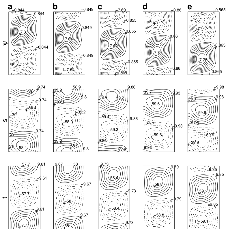
Figure 16: $\theta=\pi/2$. Viscous fluid and no-slip slot boundaries; $\eta=\chi=1$. Perturbation temporal behavior throughout nearly a half of the oscillation period $\tau_{p}\approx 46\delta\tau$ ($\delta\tau=0.05$) just beyond the onset of 2D oscillatory instability. It was obtained from the numerical simulation of evolution of the linearized Eqs. (1)—(3) in response to the initial disturbance proportional to the background state after initial time $\tau_{i}\approx 1200$ has passed; $\lambda=2$, $\mu=1$, $Ra=11226$, $Pr=6.7$, $Le=1$. With this $\tau_{i}$, all perturbation modes other than the unstable mode ($\tau_{p}\approx 46\delta\tau$) are practically negligible. $\psi$: perturbation streamlines; $s$: isolines of solute concentration perturbation; $t$: perturbation isotherms. The actual relative values of the streamfunction perturbation are equal to $10^{-3}$ times the respective values in the figure. The solid and dashed streamlines designate the clockwise and counterclockwise rotation and are equally spaced within the positive and negative streamfunction intervals, respectively. The solid and dash-dot isolines of the component perturbations are equally spaced within the positive and negative component perturbation intervals, respectively. The instability onset $Ra$ in the data underlying this figure is different from that for Fig. 15 only because a slightly different numerical formulation is used. (a) $\tau=\tau_{i}+\delta\tau$; (b) $\tau=\tau_{i}+6\delta\tau$; (c) $\tau=\tau_{i}+11\delta\tau$; (d) $\tau=\tau_{i}+16\delta\tau$; (e) $\tau=\tau_{i}+21\delta\tau$.

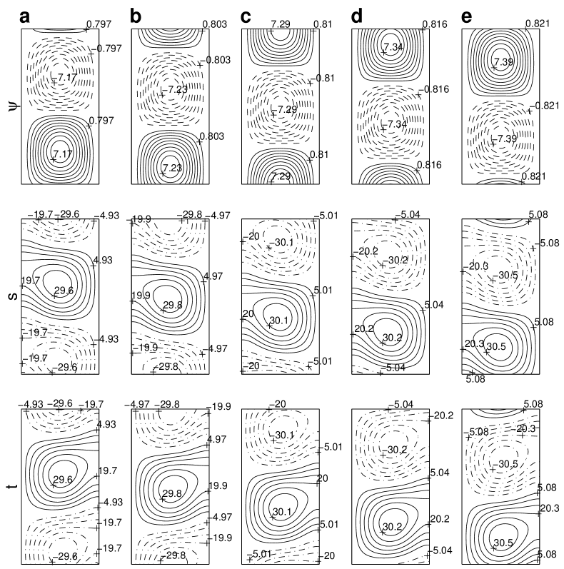
Figure 17: $\theta=\pi/2$. Viscous fluid and no-slip slot boundaries; $\eta=0$, $\chi=1$. Perturbation temporal behavior throughout nearly a half of the oscillation period $\tau_{p}\approx 51\delta\tau$ ($\delta\tau=0.05$) just beyond the onset of 2D oscillatory instability. It was obtained from the numerical simulation of evolution of the linearized Eqs. (1)—(3) in response to the initial disturbance proportional to the background state after initial time $\tau_{i}\approx 1100$ has passed; $\lambda=2$, $\mu=1$, $Ra=5586$, $Pr=6.7$, $Le=1$. With this $\tau_{i}$, all perturbation modes other than the unstable mode ($\tau_{p}\approx 51\delta\tau$) are practically negligible. $\psi$: perturbation streamlines; $s$: isolines of solute concentration perturbation; $t$: perturbation isotherms. The actual relative values of the streamfunction perturbation are equal to $10^{-3}$ times the respective values in the figure. The solid and dashed streamlines designate the clockwise and counterclockwise rotation and are equally spaced within the positive and negative streamfunction intervals, respectively. The solid and dash-dot isolines of the component perturbations are equally spaced within the positive and negative component perturbation intervals, respectively. (a) $\tau=\tau_{i}+2\delta\tau$; (b) $\tau=\tau_{i}+7\delta\tau$; (c) $\tau=\tau_{i}+13\delta\tau$; (d) $\tau=\tau_{i}+18\delta\tau$; (e) $\tau=\tau_{i}+23\delta\tau$.

The patterns illustrated in Figs. 15, 16, and 17 are traveling waves propagating in the gravity direction. Their nature can be clarified if one assumes that in the marginally unstable state, the speeds of their propagation adequately match the respective convective velocities oriented downwards. In the reference frame moving with such a pattern, the component perturbations are then transported vertically only upwards. This is the direction where the convective velocities are augmented by the moving reference frame.

The slot area behind such a propagating clockwise-(counterclockwise-)rotating cell is supplied with the temperature and solute perturbations from the region near the left (right) sidewall. The background component values are relatively high (low) there. Occupied by a counterclockwise-(clockwise-)rotating cell, such an area is thus largely characterized by the positive (negative) component perturbations (Figs. 15, 16, and 17).

Due to differential gradient diffusion, the density near the distinction boundary to the left is specified mainly by the solute perturbation there. At the similarity boundary to the right, however, the temperature and solute isolines behave identically to each other for either $\eta=\chi$ (Figs. 15 and 16). The density excess there thus has to be zero. (Due to the fixed solute sidewall values at $y=0$, this holds only approximately in Fig. 15.) For $\eta=0$ and $\chi=1$ (Fig. 17), differential gradient diffusion at the inverse boundary to the right results in the density there being specified mainly by the respective temperature perturbation.

A propagating convective cell that rotates counterclockwise (clockwise) is thus characterized by positive (negative) horizontal density differences between the streamline regions at the left and right sidewalls. This is what drives convective motion for such a cell. For $\eta=\chi$ (Figs. 15 and 16), such differences arise mainly from the positive (negative) solute perturbation at the left sidewall and zero density perturbation at the right boundary. For $\eta=0$ and $\chi=1$ (Fig. 17), they are mainly due to the positive (negative) solute and temperature perturbations at the left and right sidewalls, respectively.

Such a downwards-propagating counterclockwise-(clockwise-)rotating convective cell also has its component perturbations near the left (right) sidewall practically steady. The convective-cell velocities there are largely offset by the speed of propagation. There is thus a steady horizontal density difference that maintains the downwards propagation of such a flow pattern. For $\eta=\chi$ (Figs. 15 and 16), this difference is specified by the positive left-sidewall solute perturbation and zero right-sidewall density perturbation for a counterclockwise-rotating cell. For $\eta=0$ and $\chi=1$ (Fig. 17), the steady density difference comes from the cells rotating in both senses. It is due to the positive (negative) left-(right-) and zero right-(left-)sidewall solute (temperature) perturbation for a counterclockwise-(clockwise-)rotating cell.

Marginal-stability curves.

For any pair of $\eta$ and $\chi$ just considered at $\theta=\pi/2$, the propagating 2D convective pattern gives rise to such a distribution of the component perturbations as favors its convective motion and maintains its direction of propagation. This is implemented due to differential gradient diffusion. Such a process takes place at the distinction sidewall alone for $\eta=\chi$ and at both vertical boundaries for $\eta=0$ and $\chi=1$.

For any $\eta$ and $\chi$, the instability mechanism at $\theta=\pi/2$ is underlain by horizontal density differences accompanying the flow pattern. The independence of 2D $Ra_{c}(k_{y})$ and $\omega_{c}(k_{y})$ in Fig. 13(a) of the value of $\eta=\chi$ is therefore just a manifestation of the component disparity at the distinction boundary being unaffected by the orientation of component isolines at the similarity sidewall. Eq. (31) then suggests that such independence is retained for $k_{z}>0$ as well. Since the increase of $k_{z}$ for a fixed $k_{y}$ decreases the overall wavelength, $\omega_{c}(k_{y})$ in Figs. 13(a) and 14(a) also increases with $k_{z}$.

Convective cells driven by such across-slot density differences between their vertically moving particles make their along-slot dissipation a part of the instability feedback. Analogously to the second dissipation mechanism for standing-wave perturbation at $\theta=0$, discussed in Sec. 4.1.1 above, this causes an infinite growth of 2D $Ra_{c}(k_{y})$ with $k_{y}$ decreasing to $0$ at $\theta=\pi/2$. At $\theta=0$, such a growth for $\eta=\chi=1$ is also caused by solute diffusion at the similarity boundary. For $\eta=\chi$, the 2D marginal-stability curves at $\theta=0$ [Fig. 8(a)] are thus smoothly transformed into those at $\theta=\pi/2$ [Figs. 11,12, and 13(a)]. For $\eta=0$ and $\chi=1$ at $\theta=\pi/2$, the increase of 2D $Ra_{c}(k_{y})$ near $k_{y}=0$ is also due to neutralization of either component by diffusion. Such a marginal-stability curve for $\theta$ decreasing from $\pi/2$ to $0$ is discussed in Sec. 4.1.3 below.

Inversely affecting the component perturbations at the vertical sidewalls, differential gradient diffusion for $\eta=0$ and $\chi=1$ still leads to the respective horizontal density differences augmenting each other by their superposition. The instability for these $\eta$ and $\chi$ [Fig. 14(a)] thus sets in substantially before that for $\eta=\chi$ [Fig. 13(a)]. Such combination of the effects of differential diffusion at the boundaries also results in the convection pattern (Fig. 17) without a slope between its across-slot motion and the horizontal axis.

Such horizontality of across-slot motion, however, makes the overall cell path shorter for $\eta=0$ and $\chi=1$ than for $\eta=\chi$. With respect to the relative streamfunction amplitudes, therefore, the maximal horizontal density differences in Fig. 17 exceed those in Figs. 15 and 16. The intensity of convection in the marginally unstable state has to be matched by the speed of pattern propagation and thus by the associated $\omega_{c}(k_{y})$. This explains why $\omega_{c}(k_{y})$ are respectively smaller for $\eta=0$ and $\chi=1$ [Fig. 14(a)], where convective motion is relatively weaker, than for $\eta=\chi$ [Fig. 13(a)]. Also consistent with this argument is that the difference between such $\omega_{c}(k_{y})$ grows with $k_{y}$.

4.1.3 $\theta\in[\pi/2,\pi]$

General on 2D disturbances.

For $\theta=\pi$, the across-slot gravity is manifested as a steady instability [28, 29]. For the values of $\eta$ and $\chi$ considered in this study, such an instability is discussed in Sec. 4.2.2 below. Also characterized by steadily rotating convective cells, the 2D traveling waves arising at $\theta=\pi/2$ thus have to transform into the respective steady disturbances when $\theta$ increases above $\pi/2$. The speed of flow-pattern propagation, $\omega_{c}(k_{y})/k_{y}$, then has to decrease to $0$ for all $k_{y}$. For the reflectionally symmetric pattern of two counter-propagating waves arising at $\theta=\pi/2$ when $\eta=1$ and $\chi=0$ [32], such a decrease begins with certain $k_{y}$ at $\theta\approx 1.5\pi/2$.

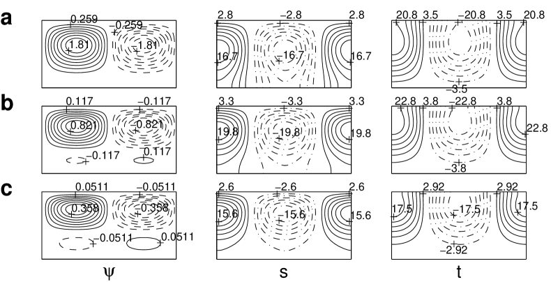
Figure 18: $\theta=0$. Viscous fluid and no-slip slot boundaries; $\eta=0$, $\chi=1$. [In light of transformation (20), these results also apply to $\theta=\pi$ if $Ra_{c}\mapsto Ra_{c}^{s}$, $Ra^{s}\mapsto Ra$, and thus $\mu\mapsto 1/\mu$.] 2D singular eigenvectors corresponding to the wavelength $\lambda=2$ at the onset of small-amplitude steady convection; $Le=1$. $\psi$: perturbation streamlines; $s$: isolines of solute concentration perturbation; $t$: perturbation isotherms. The variables are nondimensionalized as in Eqs. (1)—(3). The actual relative values of the streamfunction perturbation are equal to $10^{-3}$ times the respective values in the figure. The solid and dashed streamlines designate the clockwise and counterclockwise rotation and are equally spaced within the positive and negative streamfunction intervals, respectively. The solid and dash-dot isolines of the component perturbations are equally spaced within the positive and negative component perturbation intervals, respectively. (a) $\mu=1$, $Ra_{c}=9787$; (b) $\mu=1.3$, $Ra_{c}=25478$; (c) $\mu=1.5$, $Ra_{c}=46908$.

For the present values of $\eta$ and $\chi$, however, the mechanisms described in Sec. 4.1.2 above have to retain a flow-pattern propagation for any $\theta\in[\pi/2,\pi)$. The decrease of $\omega_{c}(k_{y})$ to $0$ for any $k_{y}$($>0$) can thus take place only when $\theta=\pi$, as in Fig. 13(b) and (c) and in Fig. 14(b). The phases of nonzero component perturbations in Figs. 15, 16, and 17 also nearly coincide with the streamfunction phases of the opposite sign. This is due to the traveling nature of such convective patterns (Sec. 4.1.2). When $\omega_{c}(k_{y})$ turns $0$ with $\theta$ reaching $\pi$, however, these relative phases have to become shifted by a quarter of the wavelength with respect to each other, as in Fig. 2 of [29] and in Fig. 18(a).

2D disturbances for $\eta=\chi$.

For $\theta=\pi/2$, the along-slot part of dissipation reduces efficiency of the instability feedback. This does not apply to $\theta=\pi$, where only the first of the two dissipation mechanisms accentuated in Sec. 4.1.1 above is relevant. In the framework of this first mechanism, however, the across-slot part of dissipation for $\eta=\chi$ is also larger at $\theta=\pi/2$ than at $\theta=\pi$. This is due to the slope of such an across-slot cell motion at $\theta=\pi/2$ (Figs. 15 and 16). For $\eta=\chi=0$, 2D $Ra_{c}(k_{y})$ is thus higher at $\theta\in[\pi/2,\pi)$ than at $\theta=\pi$ for any $k_{y}$ [Fig. 13(a) and (b)]. The difference between such $Ra_{c}(k_{y})$ also has to be infinite at any $\theta\in[\pi/2,\pi)$ as $k_{y}$[$=o(\pi-\theta)$]$\rightarrow 0$ for any ${\omega_{c}(k_{y})}_{|k_{y}\rightarrow 0}$ in Fig. 13(b), due to the effect of along-slot dissipation. Compared to ${\omega_{c}(k_{y})}_{|k_{y}\rightarrow 0}\rightarrow 0$, however, such effect is moderated when ${\omega_{c}(k_{y})}_{|k_{y}\rightarrow 0}\asymp 1$.

As $\theta$ exceeds $\pi/2$, in particular, two joined marginal-stability branches with ${\omega_{c}(k_{y})}_{|k_{y}\rightarrow 0}\rightarrow 0$ (due to the across-slot gravity) also isolatedly arise from $k_{y}=0$ [Fig. 13(b), $\theta=1.4\pi/2$]. Their higher $Ra_{c}(k_{y})$ has the slightly higher $\omega_{c}(k_{y})$. Both their $Ra_{c}(k_{y})$ are smaller and larger than that of the main branch [whose ${\omega_{c}(k_{y})}_{|k_{y}\rightarrow 0}\asymp 1$, due to the along-slot gravity] at some $k_{y}>0$ and at $k_{y}\rightarrow 0$, respectively. [${Ra_{c}(k_{y})}_{|k_{y}\rightarrow 0}\rightarrow\infty$ is assumed for the smallest $\omega_{c}(k_{y})$ as well.] Growing with $\theta$, the higher- and lower-$\omega_{c}$ branches with ${\omega_{c}(k_{y})}_{|k_{y}\rightarrow 0}\rightarrow 0$ meet the main branch at a finite $k_{y}$ and unfold with its smaller- and larger-$k_{y}$ intervals, respectively [Fig. 13(b), $\theta\geq 1.5\pi/2$]. The branch with ${\omega_{c}(k_{y})}_{|k_{y}\rightarrow 0}\asymp 1$ then exists only below such a finite $k_{y}$ as decreases to $0$ with $\pi-\theta$.

For $\eta=\chi=1$, solute diffusion at the similarity boundary increases 2D $Ra_{c}(k_{y})$ infinitely as $k_{y}$ decreases to $0$ at $\theta=\pi$ [Fig. 13(c)] (Sec. 4.2.2 below). At $\theta=\pi/2$, such $Ra_{c}(k_{y})$ is still independent of $\eta=\chi$ [Fig. 13(a)]. Its infinite increase for $k_{y}\rightarrow 0$ is then due only to the above role of along-slot dissipation. When $k_{y}$ decreases, however, the relative portion of streamline particles whose horizontal density differences drive a convective cell grows at $\theta=\pi/2$ compared to $\theta=\pi$. This efficiency factor eventually dominates the discrepancy between the growing stabilizing effect of along-slot dissipation and that of solute diffusion at the similarity boundary. The 2D $Ra_{c}(k_{y})$ near $k_{y}=0$ thus becomes smaller at $\theta=\pi/2$ [Fig. 13(a)] than at $\theta=\pi$ [Fig. 13(c)]. With $\theta$ increasing from $\pi/2$, therefore, the $Ra_{c}(k_{y})$ grows for such very small $k_{y}$ and decreases elsewhere to transform into its values at $\theta=\pi$.

2D disturbances for $\eta=0$ and $\chi=1$.

For $\eta=0$ and $\chi=1$, the across-slot gravity when $\theta=\pi$ ($\theta=0$) favors and opposes growth of steadily rotating convective cells at the distinction (inverse) and inverse (distinction) boundaries, respectively. Its effect is manifested in terms of respective along-slot density differences arising between the streamline particles moving across the slot close to these boundaries. For $\theta\in(\pi/2,\pi)$ [$\theta\in(0,\pi/2)$], it is combined with the effect of along-slot gravity. The latter effect is manifested (Fig. 17) via across-slot density differences between the streamline particles moving along the boundaries. As 2D $k_{y}\rightarrow 0$, then, $Ra_{c}(k_{y})_{|\theta=\pi/2}<Ra_{c}(k_{y})_{|\theta=\pi,0}$ [Fig. 14(b)].

Since the instability for $\theta=\pi/2$ is also due to differential gradient diffusion at both sidewalls, 2D $Ra_{c}(k_{y})$ for such $\theta$ is smaller than that of steady instability for $\theta=\pi$ ($\theta=0$) so long as the wavelength is large enough for the effect of diffusion to be dominant [Fig. 14(b)]. At $\theta=\pi$ ($\theta=0$), however, the steadily rotating convective cells are localized near the distinction (inverse) boundary [Fig. 18(a)]. The across-slot part of their dissipation thus decreases compared to $\theta=\pi/2$. With increasing $k_{y}$, the relative role of the streamline particles with along-slot density differences is also enhanced with respect to that with across-slot density differences. For sufficiently large $k_{y}$ ($k_{y}\geq 5.3$), therefore, the $Ra_{c}(k_{y})$ for $\theta=\pi$ ($\theta=0$) is smaller than that for $\theta=\pi/2$ [Fig. 14(b)].

As $\theta$ changes from $\pi/2$ to $\pi$ ($0$), the lost contribution of along-slot gravity to the intensity of the steadily rotating cells is replaced by the mutually opposing effects of across-slot gravity at the distinction and inverse boundaries. This weakens such convective motion. To maintain the remaining effect of along-slot gravity, the speed of propagation of the flow pattern has to match the relative intensity of convection. $\omega_{c}(k_{y})$ then decreases. This shifts the relative phases of component and flow perturbations with respect to each other. The portion of streamline particles with favorable across-slot density differences thus decreases, and the relative effect of along-slot gravity weakens further. The role of this feedback depends on the wavelength and $\theta$.

If the wavelength is too short for retaining a sufficiently long slot interval where the across-slot density differences matter, an efficient utilization of the along-slot gravity becomes impossible. As a consequence, the perturbation of such a wavelength occupying the whole width of the slot cannot persist. It then gives way to a convective pattern driven mainly by the across-slot gravity. Localized near the distinction (inverse) boundary, such a pattern has differently behaving $Ra_{c}(k_{y})$. These just exceed the $Ra_{c}(k_{y})$ at $\theta=\pi$ ($\theta=0$) for the relatively large $k_{y}$ in Fig. 14(b). Mainly underlain by the (steady) effect of across-slot gravity, such a pattern is also characterized by $\omega_{c}(k_{y})$ [the large-$k_{y}$ $\omega_{c}(k_{y})$ in Fig. 14(b)] that are substantially smaller than those at $\theta=\pi/2$.

For sufficiently large $|\theta-\pi/2|$, comparatively abrupt changes in $\partial Ra_{c}/\partial k_{y}$ and $\partial\omega_{c}/\partial k_{y}$ are distinguishable in Fig. 14(b). Such changes are a manifestation of the transition from the (relatively long-wavelength) convective pattern largely driven by the along-slot gravity to the localized (relatively short-wavelength) pattern mainly driven by the across-slot gravity. The longer the wavelength is (the larger is the ratio between the portions of streamline particles with across-slot and along-slot density differences) the more capable its convective pattern is of accommodating the effects of across-slot gravity without destroying the mechanism by means of which the along-slot gravity drives such convection. The abrupt changes thus arise at the smaller $k_{y}$ the more $|\theta-\pi/2|$ exceeds $0$. Their $k_{y}$ in Fig. 14(b) also tends to zero with $\theta$ approaching $\pi$ ($0$).

3D disturbances for $\eta=\chi=1$.

For $\eta=\chi=1$, solute diffusion at the similarity boundary at $\theta=\pi$ results in the $Ra_{c}(k)$ for steady instability rising to infinity with $k$ decreasing to $0$ [Fig. 13(c)], as also discussed in Sec. 4.2.2 below. Conditions I and II (Sec. 3.2.3) for three-dimensionality of the instability at small $\pi-\theta>0$ are thus met. That the instability at $\theta<\pi$ is oscillatory is consistent with the corresponding mechanism for its three-dimensionality. Such oscillatory instability with small $\omega_{c}>0$ is a perturbation of the steady instability ($\omega_{c}=0$) at $\theta=\pi$ that preserves the effects of conditions I and II.

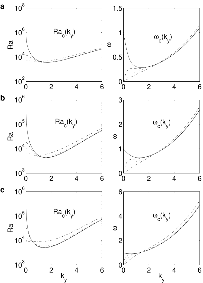
Figure 19: Viscous fluid and no-slip slot boundaries; $\eta=\chi=1$. Curves of the marginal linear stability to 3D ($k_{z}\geq 0$) oscillatory disturbances for different $k_{z}$, $Ra_{c}(k_{y})$ and $\omega_{c}(k_{y})$; $\mu=1$, $Pr=6.7$, $Le=1$. The solid lines: $k_{z}=0$, the dashed lines: $k_{z}=0.5$, the dotted lines: $k_{z}=1$, the dash-dot lines: $k_{z}=2$. (a) $\theta=1.75\pi/2$; (b) $\theta=1.5\pi/2$; (c) $\theta=1.25\pi/2$.

3D oscillatory disturbances ($k_{z}>0$) are thus most unstable near $k_{y}=0$ for small $\pi-\theta>0$ [Fig. 19(a)]. A sufficiently small $G=k_{y}/k$ in Eqs. (12) and (13) also makes the 3D effect of across-slot gravity dominant in the respectively small vicinity of $k_{y}=0$ so long as $\theta\neq\pi/2$ [Fig. 19(b),(c)]. Indeed, with $Re[d\tilde{u}(k,0)/dx]_{|\theta=\pi-o(k)}\asymp{\omega_{c}(k,0)}_{|\theta=\pi-o(k)}\asymp 1$ and $Re[d\tilde{u}(k,0)/dx]_{|\theta=\pi/2}\asymp{\omega_{c}(k,0)}_{|\theta=\pi/2}\asymp 1$ as $k\rightarrow 0$ [Fig. 13(a) and (c)], $G_{|k\rightarrow 0}=O(k)$($\rightarrow 0$) $\Longleftrightarrow[R_{\pi-o(k)}^{\pi/2}(k)/G]_{|k\rightarrow 0}\asymp[k/G]_{|k\rightarrow 0}>0$. The three-dimensionality for any $\theta\in(\pi/2,\pi)$ could be viewed as coming from conditions I and II at $G=0$ as well. As $k_{y}\rightarrow 0$ for a fixed $k_{z}>0$, in particular, the $Ra_{c}(k_{y},k_{z})|\cos\theta|$ tends to the 2D $Ra_{c}(k_{z})$ at $\theta=\pi$ [Figs. 13(c) and 19] with the ${\omega_{c}(k_{y},k_{z})}_{|k_{y}\rightarrow 0}\rightarrow 0$ (Fig. 19). This effect vanishes only when $\theta=\pi/2$, where Eq. (31) applies.

3D disturbances for $\eta=\chi=0$.

For $\eta=\chi=0$, a vicinity of $k_{y}=0$ in Fig. 20 is still dominated by 3D disturbances, despite condition II being not met at $\theta=\pi$ [Fig. 13(b)]. The role of 3D disturbances with small $k_{y}$ in Fig. 20 is also enhanced when $\theta$ decreases from $\pi$. Growing with $\pi-\theta$, the effect of along-slot dissipation on the feedback efficiency increasingly heightens the 2D $Ra_{c}(k_{y})$ in the vicinity of $k_{y}=0$. The three-dimensionality then comes from a much more unstable behavior of such $Ra_{c}(k_{y})$ at $\theta=\pi$, since the latter behavior could be mimicked by $Ra_{c}(k_{y},k_{z})_{|\theta\in(\pi/2,\pi)}$ for small $G=k_{y}/k$.

For any $k_{z}>0$, there have to exist such $k_{y}$ as make $G$ so small that the along-slot gravity in Eqs. (12) and (13) be negligible. The axes of cell rotation are then nearly parallel to the along-slot gravity. For these $k_{y}$, $\omega_{c}(k_{y},k_{z})$ and $Ra_{c}(k_{y},k_{z})|\cos\theta|$ at $\theta\in(\pi/2,\pi)$ are respectively approximated by $0$ and 2D ${Ra_{c}(k)}_{|\theta=\pi}$. In Fig. 13(b), 2D ${Ra_{c}(k)}_{|\theta=\pi}$ reaches its minimum, $720$, as $k\rightarrow 0$ [32, 49] (Sec. 4.2.2 below). For such $G$ and small enough $k_{z}$, the $Ra_{c}(k_{y},k_{z})\approx Ra_{c}(0,k_{z})\approx Ra_{c}(k_{z},0)\approx 720/|\cos\theta|$. It is thus smaller than the smallest 2D ${Ra_{c}(k_{y})}_{|k_{y}\rightarrow 0}$($\rightarrow\infty$) at $\theta\in(\pi/2,\pi)$ [Fig. 20(a),(b), Sec. 4.1.3].

The more $\theta$ initially decreases from $\pi$ the greater the smallest 2D $Ra_{c}(k_{y})$ near $k_{y}=0$ diverges from such $Ra_{c}(k_{y})_{|\theta=\pi}/|\cos\theta|$ [Fig. 13(b), $\theta\geq 1.5\pi/2$]. However, the neutralization of along-slot gravity by small $G_{|k_{z}>0}$ also makes the 3D analogue of the 2D branch with $\omega_{c}(k_{y})_{|k_{y}\rightarrow 0}\asymp 1$ to additionally connect to that of the higher-$\omega_{c}$ 2D branch with $\omega_{c}(k_{y})_{|k_{y}\rightarrow 0}\rightarrow 0$ [Fig. 20(a) and (b)]. For $k_{z}>0$, closed contours of finite $(Ra_{c},k_{y})$ and $(\omega_{c},k_{y})$ thus form at these $\theta$. Growing with $\pi-\theta$, such contours collide with the respective smaller 3D $Ra_{c}(k_{y})$ and $\omega_{c}(k_{y})$ around $\theta\approx 1.4\pi/2$ (at the smaller $\pi-\theta$ the smaller $k_{z}$ is, starting from the reorganization of the 2D branches). Via such a 3D collision, a structure with two connected limit points unfolds [Fig. 20(c)]. Its hysteresis reconciles the small- and large-$G$ small-$k_{z}$ branches of disparate 3D nature.

For small $k_{z}$, in particular, $Ra_{c}(k_{y},k_{z})$ and $\omega_{c}(k_{y},k_{z})$ are approximated by the $Ra_{c}(k_{y},0)$ and $\omega_{c}(k_{y},0)$ at the same $\theta$. Such are the upper branches in Fig. 20(c). They fail to exist only for such small $G$ (i.e., $k_{y}$ at a fixed $k_{z}$) as make the 3D effect of along-slot gravity relatively negligible. Largely triggering convection by the across-slot gravity alone, the small-$G$ nearly-steady lower branches in Fig. 20(c) fail to exist when the increase of $G$ (i.e., of $k_{y}$ at a fixed $k_{z}$) transforms the convective pattern so that it ought to be driven by the along-slot gravity as well. Some quantitative details are given in Table 2.

With $k$ decreasing along the upper branch, the 2D effect of along-slot gravity grows with respect to that of across-slot gravity, according to the relative roles of the across-slot and along-slot density differences. Neutralization of such along-slot gravity in (3D) Eqs. (12) and (13) would thus require $G$ to decrease with $k$ at the upper limit point. With $dG/dk>0$ at this limit point, $dk_{y}/dk_{z}>k_{y}/k_{z}$, analogously to (37) following from (36).

Along the (lower) branch largely specified by $k$ alone, however, $\partial G/\partial k>0\Longleftrightarrow dG/dk>0$. Arising due to the across-slot gravity alone, the lower branch thus reaches its upper bound when $G$ becomes so large that the latter inequality fails. At this bound then $dG/dk\leq 0$, as discussed in Sec. 4.1.2 of [32] for $|\tan\theta|$ and the exactly steady 2D analogue of such a branch at $\eta=1$ and $\chi=0$. For the lower limit point, therefore, $dG/dk_{z}\leq 0$ and $dk_{y}/dk_{z}\leq k_{y}/k_{z}$. This restriction leads to vanishing of the hysteresis region with increasing $k_{z}$ [Fig. 20(c) and Table 2]. Such a region also vanishes as $\theta$ approaches $\pi/2$. For $k_{z}$($>0$) being fixed, in particular, Eq. (38) at both limit points implies $\partial k_{y}(k_{z},\theta)/\partial\theta>0$ for the relevant $\theta>\pi/2$ (Table 2). For $\eta=1$ and $\chi=0$ (Fig. 10 in [32]), the exactly steady analogue of the current small-$G$ branch also shrinks to $k=0$ as $\theta$ reaches $\pi/2$.

3D disturbances for $\eta=0$ and $\chi=1$.

As discussed in Sec. 4.1.3 above, the relatively abrupt changes in 2D $\partial Ra_{c}/\partial k_{y}$ and $\partial\omega_{c}/\partial k_{y}$ for $\eta=0$ and $\chi=1$ are due to a switching between the primary roles of the two gravity components in the nature of the perturbation. They are thus specified by $\theta$ alone. With $k$ substituting for $k_{y}$, the 3D effect of along-slot gravity decreases with respect to that of across-slot gravity, due to the emergence of $G$($<1$) in Eqs. (12) and (13). The 3D boundary at which the nature of perturbation changes, $k_{y}^{\theta}(k_{z})$, thus deviates downwards from $q_{y}^{\theta}(k_{z})\equiv[{k_{y}^{\theta}(0)}^{2}-k_{z}^{2}]^{1/2}$. This is seen from Fig. 21(a) and (b) and from Table 3. When the change in 2D $\partial Ra_{c}/\partial k_{y}$ is steep enough [Fig. 21(a)], such a deviation leads to a short interval of $k_{y}$ with 3D most unstable disturbances separated from $k_{y}=0$.

Conditions I and II are met for the steady marginal-stability curve at $\theta=\pi$ ($\theta=0$) [Figs. 7 and 14(b)]. Here condition II holds due to the opposition provided by the effect of component conditions at the inverse (distinction) boundary to a steady cell rotation. For small $\pi-\theta$ ($\theta$) [Fig. 21(a)], 3D slow-propagating cells arising from the steady disturbances [localized at the distinction (inverse) boundary] are thus most unstable near $k_{y}=0$.

With $Re[d\tilde{u}(k,0)/dx]_{|\theta=\pi-o(k)}\asymp Re[d\tilde{u}(k,0)/dx]_{|\theta=o(k)}\asymp{\omega_{c}(k,0)}_{|\theta=\pi-o(k)}={\omega_{c}(k,0)}_{|\theta=o(k)}\asymp 1$ and $Re[d\tilde{u}(k,0)/dx]_{|\theta=\pi/2}\asymp{\omega_{c}(k,0)}_{|\theta=\pi/2}\asymp 1$ as $k\rightarrow 0$ [Fig. 14(b)], $G_{|k\rightarrow 0}=O(k)$($\rightarrow 0$) $\Longleftrightarrow[R_{\pi-o(k)}^{\pi/2}(k)/G]_{|k\rightarrow 0}=[R_{0+o(k)}^{\pi/2}(k)/G]_{|k\rightarrow 0}\asymp[k/G]_{|k\rightarrow 0}>0$. Such a three-dimensionality then also exists so long as $\theta\neq\pi/2$ [Fig. 21(b) and (c)], since the across-slot gravity is made dominant by a sufficiently small $G$ at any $\theta\in(\pi/2,\pi)$ [$\theta\in(0,\pi/2)$]. This three-dimensionality could be viewed as coming from conditions I and II at $G=0$ as well. As $k_{y}\rightarrow 0$ for a fixed $k_{z}>0$, in particular, the $Ra_{c}(k_{y},k_{z})|\cos\theta|$ tends to the 2D $Ra_{c}(k_{z})$ at $\theta=\pi$ ($\theta=0$) with the ${\omega_{c}(k_{y},k_{z})}_{|k_{y}\rightarrow 0}\rightarrow 0$ [Figs. 7, 14(b), and 21].

Associated in Table 3 with $k_{y}^{G}(k_{z})$, the relatively abrupt changes in $\partial Ra_{c}/\partial k_{y}$ and $\partial\omega_{c}/\partial k_{y}$ arising from $k_{y}=0$ are thus also due to a transition between the perturbation suited mainly for the across-slot gravity and that for the along-slot gravity. Such a transition is however essentially of a 3D nature.

With increasing $k$, the 2D effect of along-slot gravity decreases with respect to that of across-slot gravity. At $k_{y}^{G}(k_{z})$ for a fixed $\theta\in(\pi/2,\pi)$ [$\theta\in(0,\pi/2)$], the latter gravity component still gives way to the former in driving the perturbation. To neutralize the 2D across-slot gravity in Eqs. (12) and (13), $G$ must then grow with such $k$: $dG/dk>0$ for $k=[{k_{y}^{G}(k_{z})}^{2}+k_{z}^{2}]^{1/2}$. As (37) follows from (36), therefore, $dk_{y}^{G}/dk_{z}>k_{y}^{G}/k_{z}>0$ (Fig. 21 and Table 3). With $Re[d\tilde{u}(k,0)/dx]_{|\theta=\pi-o(k)}\asymp Re[d\tilde{u}(k,0)/dx]_{|\theta=o(k)}\asymp 1$ and $Re[d\tilde{u}(k,0)/dx]_{|\theta=\pi/2}\asymp 1$ as $k\rightarrow 0$ [$k_{z}\rightarrow 0$, $k_{y}(k_{z})=k_{y}^{G}(k_{z})=o(k_{z})$], $[R_{\pi-o(k)}^{\pi/2}(k)k/k_{y}]_{|k\rightarrow 0}=[R_{0+o(k)}^{\pi/2}(k)k/k_{y}]_{|k\rightarrow 0}\asymp 1$ implies $(k^{2}/k_{y})_{|k\rightarrow 0}\asymp 1$ for $k_{y}(k_{z})=k_{y}^{G}(k_{z})$ [$=o(k_{z})$]. Relations (35) then apply to $k_{y}^{G}(k_{z})$.

For large enough $|\theta-\pi/2|$ [Fig. 21(a) and (b)], $k_{y}^{\theta}(0)$ is distinguishable within the considered range of $k_{y}$. Since $k_{y}^{\theta}(k_{z})$ decreases with increasing $k_{z}$, the above increase of the respective $k_{y}^{G}(k_{z})$ with $k_{z}$ eventually leads to vanishing of the interval of $k_{y}$ where the instability is mainly due to the along-slot gravity. This takes place when $k_{y}^{G}(k_{z})$ and $k_{y}^{\theta}(k_{z})$ merge. When $\theta$ is so close to $\pi/2$ that such $k_{y}^{\theta}(k_{z})$ are not found [Fig. 21(c)], the increases of $Ra_{c}(0,k_{z})=Ra_{c}(k_{z})_{|\theta=0,\pi}/|\cos\theta|$ and of $k_{y}^{G}(k_{z})$ itself with large enough $k_{z}$ make the changes in $\partial Ra_{c}/\partial k_{y}$ and $\partial\omega_{c}/\partial k_{y}$ at $k_{y}^{G}(k_{z})$ indistinguishable. The slow-propagating cells localized near the distinction (inverse) boundary then smoothly transform into the traveling cells occupying the whole slot width.

As discussed above, $k_{y}^{\theta}(k_{z})$ increases when $|\theta-\pi/2|$ decreases for a given $k_{z}$. For $k_{z}$($>0$) being fixed, however, Eq. (38) implies $\partial k_{y}^{G}(k_{z},\theta)/\partial\theta>0$ [$\partial k_{y}^{G}(k_{z},\theta)/\partial\theta<0$] for $\theta\in(\pi/2,\pi)$ [$\theta\in(0,\pi/2)$]. The ultimate vanishing of the relatively abrupt changes in $\partial Ra_{c}/\partial k_{y}$ and $\partial\omega_{c}/\partial k_{y}$ thus has to take place at the larger $k_{z}$ the closer $\theta$ is to $\pi/2$, as in Fig. 21 and Table 3.

4.2 Linear steady instability for $\theta=\pi$

4.2.1 Background

Computed from Eqs. (24) and (25) and boundary conditions (14), (15), and (16), steady marginal-stability curves for $\theta=\pi$ and prescribed $Ra$ are illustrated in Figs. 22, 23, and 24. Their most unstable wave numbers, $k_{c}$, and the respective $Ra_{c}^{s}(k_{c})$ are provided in Table 4. Although Fig. 24 and its data in Table 4 are also relevant to $\theta=0$ (as mentioned in the captions of Fig. 24 and Table 4), they are discussed in Sec. 4.2.2 below only in terms of $\theta=\pi$. The shape of the presented curves is specified by the combined effects of across-slot diffusion and the first dissipation mechanism (Sec. 4.1.1).

For $Ra=0$, such diffusion is stabilizing. Since it is absent for $\chi=0$, the most unstable wave number is zero, where the minimal effect of the first dissipation mechanism is achieved. Derivable via the long-wavelength expansion [49, 50], the respective $Ra_{c}^{s}(0)$ (Fig. 22 and Table 4) depends on the velocity conditions at the slot boundaries.

For $\chi=1$, the stabilizing effect of diffusion for $Ra=0$ renders the most unstable wavelength finite. Compared to the stress-free boundary condition, the enhancement of along-slot dissipation at a no-slip boundary reduces the across-slot portion of actively moving streamline particles with an along-slot density difference. Like diffusion, the effect of such disparity in along-slot dissipation is also augmented with the wavelength. Besides raising $Ra_{c}^{s}(k)$ for all $k$, therefore, the no-slip effect increases $k_{c}$ as well (Figs. 23 and 24 in Table 4 for $Ra=0$) [49, 50]. The smaller across-slot portion of streamline particles driving convection then constitutes a larger part of the overall streamline.

When introduced only at one boundary for $Ra=0$, the no-slip effect is more pronounced in combination with the flux solute condition, where the solute perturbation isolines are orthogonal to the boundary [Figs. 23(b) and 24(b), and Table 4]. This takes place because for the stress-free condition, the actively moving streamline particles with along-slot density differences exist infinitesimally close to the boundary at which there is no diffusion. The (zero-$Ra$) $k_{c}$ in Table 4 ($\chi=1$) for $\gamma_{-}=1$ and $\gamma_{+}=0$ ($\gamma_{-}=0$ and $\gamma_{+}=1$) is thus closer to its value for $\gamma_{\pm}=1$ ($\gamma_{\pm}=0$) than to that for $\gamma_{\pm}=0$ ($\gamma_{\pm}=1$) [49, 50].

4.2.2 $Ra>0$

$\eta=\chi=0$.

When $Ra$ increases from $0$, the effect of diffusion becomes destabilizing. Being due to differential gradient diffusion at the distinction boundary, the instability mechanism is then similar to that described in [28, 29]. For $\eta=\chi=0$, its effect is maximized at the infinite wavelength, where any stable fixed-value stratification is fully neutralized by diffusion. Also minimizing the role of the first dissipation mechanism, such wavelength thus remains most unstable for any $Ra$ [49]. For $k\rightarrow 0$, the instability parameters in Fig. 22 (Table 4) are identical to those for $\eta=1$ and $\chi=0$ [28, 29, 32, 49, 51].

When $k$ increases from $0$, however, quantitative differences from the respective $Ra_{c}^{s}(k)$ for $\eta=1$ and $\chi=0$ arise, due to differential gradient diffusion taking place only at one boundary. In Fig. 22(b), such differential diffusion at the distinction boundary is also more effective in combination with the respective stress-free single boundary condition ($\gamma_{-}=0$ and $\gamma_{+}=1$) than with the no-slip one ($\gamma_{-}=1$ and $\gamma_{+}=0$). As discussed above, the (nondiffusive) flux component perturbation is affected by the disparity between the no-slip and stress-free velocity conditions more than the (diffusive) fixed-value one.

$\eta=\chi=1$.

When coupled with the distinction boundary, the single stress-free condition is more destabilizing than in its combination with the similarity boundary for $\eta=\chi=1$ as well. In particular, this explains the relative location of the solid and dashed lines in Fig. 23(b). With growing $Ra$, in addition, the $Ra_{c}^{s}(k_{c})$ in Table 4 for $\gamma_{-}=0$ and $\gamma_{+}=1$ becomes even much closer to such a value for $\gamma_{\pm}=0$ than to that for $\gamma_{-}=1$ and $\gamma_{+}=0$. Likewise, such a $Ra_{c}^{s}(k_{c})$ for $\gamma_{-}=1$ and $\gamma_{+}=0$ becomes much closer to its respective value for $\gamma_{\pm}=1$ than to that for $\gamma_{-}=0$ and $\gamma_{+}=1$.

That the effect of diffusion turns destabilizing when $Ra$ increases from $0$ is also manifested for $\eta=\chi=1$ in decreasing $k_{c}$ (Fig. 23 and Table 4). Due to solute neutralization by its diffusion at the similarity boundary, however, $k_{c}$ cannot decrease to zero. It is the balance between the overall differential effect of both boundaries on component perturbations and the effect of the similarity boundary on solute perturbation that specifies the value of $k_{c}$.

As the overall effect of differential diffusion is augmented with growing $Ra$, however, the ratio of $Ra_{c}^{s}(k)$ to $Ra$ decreases for any $k$. This relatively enhances the effect of the similarity boundary on solute perturbation in the above balance specifying $k_{c}$, at which $Ra_{c}^{s}(k)/Ra$ is the smallest for a fixed $Ra$. When the latter effect turns dominant above certain $Ra$, $k_{c}$ begins to increase. As in Table 4, such an oscillatory behavior of $k_{c}$ has to be most pronounced for $\gamma_{\pm}=0$, where diffusion is not restricted by dissipation at the boundaries. It has to be least pronounced for $\gamma_{\pm}=1$, where $k_{c}=0.86$ for $Ra=200000$.

$\eta=0$ and $\chi=1$.

For $\eta=0$ and $\chi=1$ (Fig. 24), the increase of $Ra$ from $0$ introduces differential gradient diffusion that favors both a steady perturbation at the distinction boundary and a standing-wave perturbation at the inverse boundary. Such a diffusion process at the latter boundary thus opposes a steady rotation of the convective cells. As suggested by Fig. 7, however, the steady linear instability for $\gamma_{-}=\gamma_{+}$ is expected to precede the oscillatory one. (As indicated in the captions of Figs. 7, 18, and 24, the results for $\theta=0$ and for $\theta=\pi$ are relevant to each other.) Whereas both dissipation mechanisms accentuated in Sec. 4.1.1 above damp the oscillatory (standing-wave) perturbation, only the first one of them damps the steady perturbation.

Let the velocity conditions be either the same at both boundaries ($\gamma_{-}=\gamma_{+}$) or such as the single stress-free condition is at the distinction boundary ($\gamma_{-}=0$ and $\gamma_{+}=1$). Localization of steady convective cells near the distinction boundary is thus favored even when $Ra$ is small. (For $\theta=0$, such a localization at the inverse boundary is seen in Fig. 18.) The destabilizing effect of the distinction boundary then dominates the stabilizing effect of the inverse boundary. Thus $k_{c}$ only decreases with $Ra$ increasing from $0$ for such $\gamma_{\pm}$ (Table 4).

When the single stress-free condition is at the inverse boundary ($\gamma_{-}=1$ and $\gamma_{+}=0$), however, the effect of differential gradient diffusion at the distinction boundary may not be dominant. At small $Ra$, in particular, the onset of steady convection is dominated by the disparity between the velocity boundary conditions. Indeed, the overall effect of diffusion on steady convection at $Ra=1000$ remains stabilizing: ${Ra_{c}^{s}(k_{c})}_{|Ra=1000}=1949>Ra+{Ra_{c}^{s}(k_{c})}_{|Ra=0}=1000+817$ (Table 4).

For $\gamma_{-}=1$ and $\gamma_{+}=0$, $k_{c}$ thus first grows with $Ra$ increasing from $0$ (to at least $1000$, as in Table 4). Only when the stable fixed-value stratification becomes large enough, the overall effect of differential gradient diffusion on steady convective cells becomes destabilizing. With the cells localized near the distinction boundary, in particular, $k_{c}$ decreases as $Ra$ increases to $5000$ and above (Table 4). For all pairs of $\gamma_{\pm}$, however, its decrease to $0$ is still prevented by the stabilizing effect of the inverse boundary. At the infinite wavelength, such effect becomes commensurate with the destabilizing role of the distinction boundary.

Compared to the no-slip boundary condition, the stress-free condition enhances differential gradient diffusion at its boundary, as discussed above. Such an enhancement is also more relevant at the boundary where the convective cells are driven. In particular, the dashed lines are above the respective solid lines in Fig. 24(b). For growing $Ra$, in addition, $Ra_{c}^{s}(k_{c})$ for $\gamma_{-}=0$ and $\gamma_{+}=1$ remains closer to such a value for $\gamma_{\pm}=0$ than to that for $\gamma_{-}=1$ and $\gamma_{+}=0$. The $Ra_{c}^{s}(k_{c})$ for $\gamma_{-}=1$ and $\gamma_{+}=0$ also remains closer to such a value for $\gamma_{\pm}=1$ than to that for $\gamma_{-}=0$ and $\gamma_{+}=1$ (Table 4 for Fig. 24).

4.3 Finite-amplitude steady convection for $\theta=0$

4.3.1 $\eta=\chi=1$

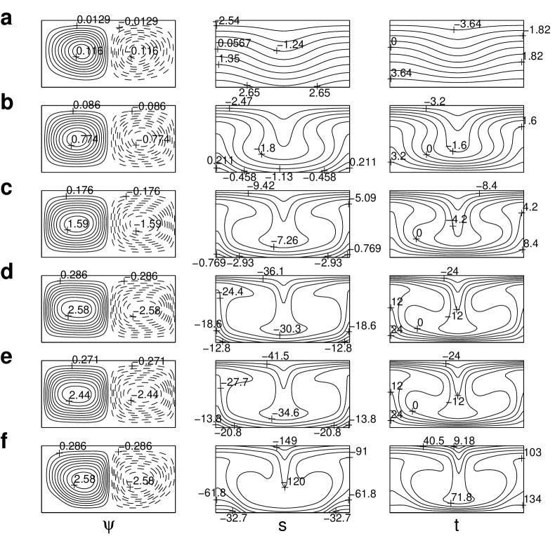
Figure 26: $\theta=0$. Viscous fluid and no-slip slot boundaries; $Pr=6.7$, $Le=1$, $\lambda=2$. 2D convective steady flows. $\psi$: streamlines; $s$: isolines of solute concentration; $t$: isotherms. The solid and dashed streamlines represent the clockwise and counterclockwise rotation and are equally spaced within the positive and negative streamfunction intervals, respectively. The actual values of $s$ and $t$ are equal to $10^{3}$ times the respective values in the figure. (a)—(e): $\eta=\chi=1$. (a) $\mu=0.7$, $Ra=9107$, branch $A1$; (b) $\mu=0.7$, $Ra=8000$, branch $A2$; (c) $\mu=1$, $Ra=24000$, branch $A2$; (d) $\mu=1.3$, $Ra=60000$, branch $A2$; (e) $\mu=1.5$, $Ra=60000$, branch $A2$; (f) $\eta=\chi\approx 0.41$, $\mu=1$, $Ra=300000$, branch $A2$.

For the component conditions being different only at one boundary and $\theta=0$, the most pronounced manifestation of the finite-amplitude steady instability mechanism reported for $\eta=1$ and $\chi=0$ in [37] takes place when $\eta=\chi=1$. Its bifurcation diagram is illustrated in Fig. 25. When the relative role of stable solute stratification increases with $\mu$, the linear steady instability is delayed for two reasons. One of them is merely the stabilizing solute contribution to the overall background stratification. The other reason is of a double-component nature. It is the opposition provided by differential gradient diffusion to a steady rotation of convective cells. Such finite-amplitude convection is however relatively little affected by the growing solute stratification, due to the nature of its mechanism. This nature is illustrated in Fig. 26.

As the convection amplitude increases [Fig. 26(a),(b)], a growing number of solute isolines near the distinction boundary are found to be ”outside” the flow domain. This effect is particularly pronounced in the regions of across-slot motion towards this boundary. The background solute scale is thus reduced in the convective state. Due to the fixed-value temperature conditions at both boundaries, however, the isotherms only increase their density in the direction of across-slot motion near either boundary. The background temperature scale thus remains intact even when convection is well-developed [Fig. 26(b)—(e)].

Substantially reducing the across-slot solute scale, the finite-amplitude perturbation thus generates such unstable density gradients in the regions of across-slot motion [Fig. 26(a)—(e)] as exceed the linear single-component threshold [$Ra_{c}(\pi)\approx 1707$ [52]]. This takes place well before onset of the double-component linear instability (Fig. 25). Horizontal density differences between the respective streamline points are then formed and give rise to (positive) convective feedback. Coming from finite-amplitude Rayleigh—Benard convection, this feedback maintains the disparity between component gradients.

Such finite-amplitude convection also arises when the overall background stratification is neutral or stable. For the present formulation, the linear steady instability is then absent [Fig. 26(c)—(e)]. With limit point $L$ in Fig. 25 moving to higher $Ra$ for growing $\mu$, the flow amplitude and the disparity between component scales at the same $Ra$ ($=60000$) still decrease [Fig. 26(d),(e)].

Continuation of such a finite-amplitude steady flow for $\mu=1$ in $\theta$ to $\theta>0$ fails even when the step in $\theta$ is close to zero. Such a failure of the continuation procedure is also experienced when an attempt to continue a supercritical finite-amplitude steady solution for $\mu=1$ and $\theta=\pi$ to $\theta<\pi$ is made. The latter failure has to be due to the anticipated transformation of the steady finite-amplitude solutions into traveling-wave ones, as discussed for the respective small-amplitude flows say in Sec. 4.1.3 above. Purely finite-amplitude transformations of a traveling wave into a steady flow have been reported in binary-fluid convection [53] and in conventional double-diffusive convection [54]. The continuation failure at $\theta=0$ could thus also be due to a transformation of the steady finite-amplitude flow into a traveling-wave one.

4.3.2 Comparison with $\eta=1$ and $\chi=0$ and $\eta=\chi<1$

Differential gradient diffusion at both boundaries delays the linear steady instability for $\theta=0$ more effectively than this process at the distinction boundary alone. In the finite-amplitude manifestation of steady convection, the enhancement of differential diffusion on account of the second boundary also plays a stabilizing role. Solute stratification is however substantially reduced in such a convective steady state. Being partly due to differential gradient diffusion, its (stabilizing) effect on finite-amplitude steady convection is then much smaller than that on the respective small-amplitude one. When $\mu<1$, the hysteresis thus has to be more pronounced for $\eta=1$ and $\chi=0$ than for $\eta=\chi=1$.

In particular, the interval of hysteresis is larger for $\mu=0.6$ in Fig. 2 of [37] than for $\mu=0.7$ in the present Fig. 25 (see also Table 5). Limit point $L$ for $\eta=\chi=1$ still precedes that for $\eta=1$ and $\chi=0$ at the same $\mu$. Compared to $\eta=\chi=1$, the stabilizing effect of differential gradient diffusion on finite-amplitude steady convection is enhanced for $\eta=1$ and $\chi=0$ more than the efficiency of such finite-amplitude instability. [Indeed, the convection amplitude in Fig. 26(c) is slightly higher than that in Fig. 4(c) of [37].] For this reason, limit point $L$ for $\eta=\chi=1$ continues to precede that for $\eta=1$ and $\chi=0$ at least when $\mu\in[1,1.5]$, where the linear steady instability sets in at infinite $Ra$ in both these cases. In particular, this is seen from Fig. 2 (including the caption) in [37] and the present Fig. 25 for $\mu=1$ and $\mu=1.5$.

[Regarding the solute scale and phase specification, the present numerical formulation for $\eta=\chi=1$ (Sec. 2.1) is not identical to that in [37]. Using the same steady solution phase and no other restrictions, however, it is most consistent with the formulation in [37]. The above relative location of limit point $L$ for $\eta=\chi=1$, with respect to that for $\eta=1$ and $\chi=0$, was also found to take place when the solute concentration values are fixed at the middle points of the slot boundaries in both cases.]

The finite-amplitude mechanism discussed in Sec. 4.3.1 above is underlain by the flux condition decreasing in the perturbed state the across-slot scale of a component on which it is imposed at a boundary. The across-slot perturbation scales of both components then have to be substantially smaller for $\eta=\chi=0$ than for $\eta=\chi=1$. The resulting smaller disparity between such scales is thus generally less likely to trigger finite-amplitude steady convection before the onset of small-amplitude one. This explains why, for $\gamma_{\pm}=1$, the hysteresis practically vanishes when $\eta=\chi$ approaches $0$ at least for $\mu\leq 0.9$.

When $\eta=\chi<1$ is sufficiently above $0$, however, the hysteresis region persists. In particular, it is indisputably present at least for $\eta=\chi\approx 0.41$ (Table 5, $\gamma_{\pm}=1$). Such a finite-amplitude steady flow is illustrated in Fig. 26(f). As discussed in Sec. 4.2.2 above, differential gradient diffusion is also more effective at a stress-free slot boundary than at a no-slip one. Disparity between the small- and finite-amplitude manifestations of such a process is an important factor for the bifurcation subcriticality. The stress-free boundary conditions thus ought to have a quantitative effect on the hysteresis region.

For $\mu\leq 1$ (Table 5), in particular, the subcriticality for $\eta=\chi\approx 0.41$ is more pronounced for $\gamma_{\pm}=0$ than for $\gamma_{\pm}=1$. (The potentially interesting cases $\gamma_{-}\neq\gamma_{+}$ are outside the scope of this work.) Trial computations with $\gamma_{\pm}=0$ at $\mu\in[0.7,0.9]$ also suggested that such a hysteresis then survives for $\eta=\chi=0$ as well. However, the latter finding could not be ascertained because of a numerically transcritical manifestation of the hysteresis at $\eta=\chi=0$. This ought to be due to an unfolding of the bifurcation diagram by the scale-fixing condition, to which the formulation for $\eta=\chi=0$ is particularly sensitive.

4.3.3 Environmental implications

Let $Ra$ in Fig. 25 be fixed on branch $A2$ above limit point $L$. This implies a value of $\mu$ where bifurcation point $B$ is subcritical. For such a flow, let $\mu$ (and $Ra^{s}$) be varied from a negative value to the (positive) value just defined and above. Fig. 25 then suggests the existence of hysteresis in $\mu$ as well. One could thus also expect such a hysteresis to arise when $Ra$ and $Ra^{s}$ are independent of each other. In particular, it ought to take place when $Ra^{s}$ is varied sufficiently for $Ra$ being fixed on the higher-amplitude branch of the respective limit point.

Viewed as a possible explanation of abrupt climate changes [22, 23], such a behavior has been reported in numerous model studies of the global ocean thermohaline circulation and climate [20, 21, 23, 24]. In these studies, the fresh-water flux into a North Atlantic ocean region of deep sinking (deep-water formation) is a parameter controlling the salt stratification there.

[Hysteresis was also found for salinity- and temperature-driven regimes of a box model considered in [15]. The boundary condition for a component is then specified by the component conductivity at the boundary. Such hysteresis is viewed as a simplified illustration of multiplicity of the regimes of global ocean thermohaline circulation and climate [16, 20, 21, 22, 23, 24]. The boxes in [15] can however represent the upper and lower ocean layers. The mechanisms of the salinity- and temperature-driven regimes [15] are then conceptually analogous to the hydrodynamic mechanisms of double-component convection in [28, 29] (Secs. 4.2.2 and 4.2.2 above) and in [37] (Secs. 4.3.1 and 4.3.2 above), respectively.

In the framework of such analogy, in particular, the difference between box values of either component corresponds to the component gradient in the respective convective state and the rate of hydraulic flow to the convection amplitude. The external mechanical mixing is also represented by the (equal) component eddy diffusivities. (If one disregards the physical dissimilarity between component boundary conductivities and their fluid diffusivities, such an analogy could also be respectively extended to the small- [1] and finite-amplitude [2] steady instabilities in conventional double-diffusive convection.)]

A basic constituent of the global ocean thermohaline circulation is comprised by the so-called Atlantic Meridional Overturning Circulation (AMOC). Operation of AMOC implies the existence of a North Atlantic region of deep sinking [17, 20, 22, 23]. Such a region also gives rise to penetration of horizontal sea-surface density differences into the ocean depth, without which AMOC could not be effectively driven by buoyancy [20, 55, 56, 57]. In the context of [55] discussed in [20, 56, 57], therefore, the nature of an AMOC driven by buoyancy could only be such as suggests no source of the AMOC hysteresis other than the sinking region. The convection hysteresis, if any, in this region thus has to be a local factor imposing the solution structure and the parameters of hysteresis on the entire AMOC (and the respective climate regimes [22, 23, 24]).

Allowing for transformation (10), however, a hysteresis between steady regimes in the convection region is certain if there is a hydrodynamic formulation where the temperature condition at a relevant boundary other than the sea-surface boundary is far enough from the flux type, as discussed above. Such a formulation could arise for the flow domain just above the bottom topography. Hysteresis in convection then ought to exist regardless of its parameters near $\eta=\chi=0$ for the stress-free boundaries if the eddy diffusivity (defined without convection) within the topographic bottom layer is not too small compared to that within the upper flow domain itself. This involves the issue of vertical variation of such an eddy diffusivity. With many uncertainties, its discussions [20, 56, 58] still seem to suggest that the lower boundary condition has to be within the range of existence of a significant hysteresis.

5 Summary and concluding remarks

5.1 General

This work provides a comprehensive insight into the manifestation of double-component convection due to different boundary conditions in a diversely oriented infinite slot when the reflection symmetry between the slot conditions for a component is broken. In a class of the addressed problems, different component conditions at one slot boundary (the distinction boundary) are considered primarily with flux and with fixed-value conditions for both components at the other (the similarity boundary). Another class of the problems is such as the component conditions at the second boundary (the inverse boundary) differ from each other inversely to the distinction boundary. For elimination of other physical effects, the primary focus is on the compensating background gradients and equal component diffusivities. Mainly treating small-amplitude convection, this study also examines finite-amplitude steady instability.

Being imposed only at one slot boundary, different component conditions still give rise to double-component convection for any slot orientation to the gravity. They also do so being inversely prescribed at the boundaries, although either component then has one fixed-value and one flux boundary condition. In either of these problem classes, however, the manifestation of small- and finite-amplitude convection is substantially disparate from that with the reflectionally symmetric boundary conditions for a component.

One aspect of such a disparity can be interpreted as coming from dissimilar 2D small-amplitude convection patterns and the ranges of their formation. It is largely a consequence of only one traveling wave being relevant when the slot orientation differs from horizontal. Another cause of the disparity is a more frequent dominance of 3D small-amplitude disturbances, due to both a previously identified three-dimensionality mechanism and new ones. Directly underlying these factors, the broken symmetry also has major implications for finite-amplitude steady instability.

5.2 Inviscid fluid

When the similarity boundary is of the flux type ($\eta=\chi=0$), the behavior of an inviscid oscillatory marginal-stability curve in the horizontal slot for $\theta=0$ is least dissimilar from that under the reflectionally symmetric component boundary conditions ($\eta=1$ and $\chi=0$). In particular, such a linear stability boundary is characterized by the most unstable wave number being zero. For independently prescribed $Ra^{s}$, $Ra_{c}$ and $\partial\omega_{c}/\partial k$ at $k=0$ obtained from the long-wavelength expansion also differ from the symmetric case only by the denominator in the expression for the former parameter. Compared to $\eta=1$ and $\chi=0$, the lack of temperature diffusion at the similarity boundary for $\eta=\chi=0$ stabilizes most wavelengths. However, it also destabilizes such long wavelengths as effectively neutralize the temperature scale by diffusion at the distinction boundary alone.

As at $\eta=1$ and $\chi=0$, the zero wave number at $\eta=\chi=0$ remains most unstable for the compensating background gradients up until the slot orientation becomes nearly vertical. For $\theta>0$, however, the reflection asymmetry of oscillatory perturbation leads to the expression relating 2D $Ra_{c}$ and $\partial\omega_{c}/\partial k_{y}$ at $k_{y}=0$ being entirely dissimilar from that for $\eta=1$ and $\chi=0$. In addition, zero limit of the $Ra_{c}(k_{y})$ and $\omega_{c}(k_{y})$ as $\theta\rightarrow\pi/2$ does not necessarily imply that the oscillatory marginal-stability boundary transforms into a steady one. For any $\theta\in[0,\pi)$, no steady linear instability arises in viscous fluid at finite $Ra_{c}$ for either $\eta=\chi$. The inviscid instability with $Ra_{c}=\omega_{c}=0$ for $\theta\geq\pi/2$ could not thus be underlain by viscous steady instability. This also applies to other such inviscid oscillatory-instability zero thresholds for $\theta\in(0,\pi)$.

Despite the absence of dissipation, the most unstable wave number for the oscillatory instability at $\theta=0$ becomes finite both when $\eta=\chi=1$ and when $\eta=0$ and $\chi=1$. For $\eta=\chi=1$, such a change comes only from solute diffusion at the similarity boundary. For $\eta=0$ and $\chi=1$, it is due to differential gradient diffusion at the inverse boundary [or at the distinction boundary for $\theta=\pi$, allowing for (20)]. When the stable gradient is independently prescribed, either of such dissimilar diffusion processes still also prevents a manifestation of the oscillatory instability in an immediate vicinity of $k=0$.

For $\eta=0$ and $\chi=1$ at $\theta=0$ and $\theta=\pi$, however, the vanishing of oscillatory instability with decreasing $k$ is also preceded by a short interval of $k$ where a higher unstable gradient of one component destabilizes the lower stable stratification of the other. This is attributed to the growing relative disparity between the oscillation frequencies at such different stable stratifications as these frequencies decrease with the increasing wavelength. Differential diffusion at the boundary favoring steady convection is thus enhanced relatively stronger by the lower stable stratification. At small enough $k$, the unstable gradient is then affected more by such stabilizing enhancement than by the effect of the stable stratification at the boundary favoring oscillatory convection.

When $\theta=0$ in inviscid fluid, solute diffusion at the similarity boundary for $\eta=\chi=1$ allows to meet (the second of) two general conditions for three-dimensionality of instability disturbances formulated in [32]. Due to these conditions, herein referred to as conditions I and II, such a three-dimensionality then arises in the vicinity of $k_{y}=0$ for small $\theta>0$. As $\theta$ increases further to $\pi/2$, however, 2D $Ra_{c}(k_{y})$ and $\omega_{c}(k_{y})$ for the compensating background gradients decrease to zero when $\eta=\chi=1$ as well. It is also the vicinity of $k_{y}=0$ that is most sensitive to the direct effect of along-slot gravity, and thus experiences the fastest decrease of 2D $Ra_{c}(k_{y})$ and $\omega_{c}(k_{y})$. Unlike other 3D instability manifestations resulting from conditions I and II, therefore, the present three-dimensionality is not retained above small $\theta>0$.

In contrast to the above problems for $\eta=\chi$, an interval of zero 2D $Ra_{c}(k_{y})$ and $\omega_{c}(k_{y})$ arises for $\eta=0$ and $\chi=1$ under the compensating background gradients already when $\theta$ ($\pi-\theta$) is infinitesimal. [Invariance (20) also makes $\theta\in(0,\pi/2)$ for $\eta=0$ and $\chi=1$ at $\mu=1$ equivalent to $(\pi-\theta)\in(0,\pi/2)$.] Expanding with growing $\theta$ ($\pi-\theta$), this interval becomes infinite as $\theta\rightarrow\pi/2$. As its lower limit also increases with $\theta$ ($\pi-\theta$), however, the $Ra_{c}(k_{y})$ and $\omega_{c}(k_{y})$ below such a limit are left finite for any $\theta\in(0,\pi/2]$ [$\theta\in[\pi/2,\pi)$]. Neutralizing either component by diffusion, such relatively long wavelengths prohibit the 2D instability manifestation at infinitesimal $Ra(k_{y})$.

The upper limit of the interval of zero 2D $Ra_{c}(k_{y})$ and $\omega_{c}(k_{y})$ thus formed for $\eta=0$ and $\chi=1$ when $\theta\in(0,\pi/2]$ [$\theta\in[\pi/2,\pi)$] is interpreted as resulting from a competition between two dissimilar patterns. Arising for the relatively longer wavelengths, one of them has steadily rotating cells driven by both the along-slot gravity and the effect of across-slot gravity at the inverse (distinction) boundary. It is a traveling wave whose speed turns infinitesimal when $Ra_{c}(k_{y})=\omega_{c}(k_{y})=0$. The other pattern is featured by cells whose sense of rotation changes periodically in time. Characterized only by finite $Ra_{c}(k_{y})$ and $\omega_{c}(k_{y})$, it arises from the effect of across-slot gravity at the distinction (inverse) boundary for the relatively shorter wavelengths.

Although conditions I and II are met in inviscid fluid at $\theta=0$ ($\theta=\pi$) for $\eta=0$ and $\chi=1$ as well, 3D instability then arises for $\theta\in(0,\pi/2)$ [$\theta\in(\pi/2,\pi)$] largely from more pronounced effects. Two of these effects are due to the 2D interval with $Ra_{c}(k_{y})=\omega_{c}(k_{y})=0$. One of them is underlain by an invariance [Eq. (31)] of the linear stability equations at $\theta=\pi/2$. With the 2D area of $Ra_{c}(k)=0$, this invariance leads to an interval of $k_{y}$ where 3D disturbances are most unstable for $\theta=\pi/2$. Such an interval thus arises at small $|\pi/2-\theta|$ as well. For any $\theta\in(0,\pi/2)$ [$\theta\in(\pi/2,\pi)$], however, 3D disturbances are also dominant due to their unequal effect on the two gravity components. Relatively reducing the along-slot gravity by $G=k_{y}/k$, this effect shifts the 3D zero-threshold interval of $k_{y}$ below such (2D) interval specified by $\theta$ alone.

3D most unstable disturbances in inviscid fluid for $\eta=0$ and $\chi=1$ also arise from another type of 3D areas with zero $Ra_{c}(k_{y},k_{z})$ and $\omega_{c}(k_{y},k_{z})$. Such a 3D area has no 2D progenitor. Taking place at any $\theta\in(0,\pi/2)$ [$\theta\in(\pi/2,\pi)$], such a perturbation three-dimensionality is still consistent with conditions I and II when they are considered at $G=k_{y}/k=0$. The nature of the zero-threshold area underlying such a 3D instability is interpretable in terms of the analogy between the effect of $G$ in the 3D marginal-stability equations for $k$ and the effect of $|\tan\theta|$ in the 2D equations for $k_{y}$. With this analogy, differential behavior of the boundaries of such an area with respect to $k_{z}$ and $\theta$ is consistent with the respective numerical data. It also matches the asymptotic behavior of the area boundaries for $k_{z}\rightarrow 0$ obtained by an independent approach.

5.3 Viscous fluid

For all the considered combinations of $\eta$ and $\chi$, oscillatory linear instability also arises in viscous fluid. When $\theta=0$, in particular, the marginal-stability curve for either $\eta=\chi$ is characterized by an infinite increase of $Ra_{c}(k)$ with $k$ decreasing to $0$. Both such increases come from reduction of the instability feedback efficiency by along-slot dissipation. First identified for $\eta=1$ and $\chi=0$ in [32], this mechanism of efficiency reduction is herein referred to as the second dissipation mechanism. For $\eta=\chi=1$, however, the long wavelengths are also so stabilized by solute diffusion at the similarity boundary.

The viscous instability at $\theta=0$ for $\eta=\chi=1$ still precedes that for $\eta=\chi=0$ so long as $k$ is not too large: $\delta Ra_{c}(k)>0$ for such $k$. Compared to $\eta=\chi=0$, diffusion of both components at the similarity boundary then leads to efficiency of the instability mechanism for $\eta=\chi=1$ being higher. Such higher efficiency, however, generates steeper velocity gradients and thus more dissipation. Relatively increasing with $k$, this effect of dissipation eventually dominates the effect of diffusion at the similarity boundary. $\delta Ra_{c}(k)$ thus changes its sign. With $k$ increasing further, it also exhibits decaying oscillations. The oscillatory behavior results from an additional dissipation arising above a value of $k$ where $\delta Ra_{c}(k)=0$ acting against the increase of $|\delta Ra_{c}(k)|$. The additional dissipation is greater for such $\eta=\chi$ as has the higher efficiency of the combined effects of diffusion and dissipation at the given $k$.

The second dissipation mechanism is the reason why oscillatory linear instability for $\eta=0$ and $\chi=1$ at $\theta=0$ and $\theta=\pi$ is preceded by the steady one. For sufficiently long wavelengths, such oscillatory instability at $\theta=0$ is preceded by those for $\eta=\chi$ as well. The stabilizing effect of the inverse boundary for $\eta=0$ and $\chi=1$ is then more important than the cell localization near the distinction boundary. As the wave number increases, however, the role of this stabilizing effect diminishes. Compared to $\eta=\chi$, the cell localization for $\eta=0$ and $\chi=1$ also leads to a faster growth of the relative portion of fluid particles with along-slot density differences, and thereby to the faster enhancement of efficiency of the instability mechanism. Above certain $k$, therefore, the oscillatory instability for $\eta=0$ and $\chi=1$ at $\theta=0$ precedes those for $\eta=\chi$.

In viscous fluid, conditions I and II are met at $\theta=0$ for either $\eta=\chi$. In both cases, 3D disturbances are thus most unstable in a vicinity of $k_{y}=0$ when $\theta>0$ is small. For either $\eta=\chi$, however, 3D disturbances with small $k_{y}$ also remain the first to arise so long as $\theta<\pi/2$. This takes place because a sufficiently small $G=k_{y}/k$ renders the effect of across-slot gravity dominant at any $\theta\in(0,\pi/2)$. Compared to the inviscid fluid for $\eta=\chi=1$, this is possible due to the respective viscous 2D effects of along-slot gravity being near $k=0$ sufficiently weak relatively to those of across-slot gravity.

In viscous fluid, the broken symmetry between boundary conditions for a component is manifested most commonly at $\theta=\pi/2$. Oscillatory instability is then characterized by a sequence of 2D counter-rotating convective cells propagating with a nonzero speed in the gravity direction. For any pair of considered $\eta$ and $\chi$, the respective propagating pattern gives rise to such a distribution of the component perturbations as favors its convective motion and maintains the direction of its propagation. This direction is sustained by a nearly steady horizontal density difference generated between the traveling convective pattern and slot boundaries. Such a mechanism of traveling-wave instability is underlain by differential gradient diffusion.

Although differential gradient diffusion for $\eta=0$ and $\chi=1$ acts inversely at the slot boundaries, its sidewall effects at $\theta=\pi/2$ match each other in the framework of the above features of the instability pattern. Such inversely symmetric effects of differential diffusion at $\theta=\pi/2$, however, result in horizontality of across-slot convective motion, in contrast to $\eta=\chi$. The corresponding reduction of the across-slot cell path then leads to a smaller relative convection amplitude of the instability. As a consequence, the marginal-stability frequencies are respectively lower for $\eta=0$ and $\chi=1$ than for $\eta=\chi$.

Horizontal density differences comprise the key quantitative feature of the vertical-slot instability mechanism. Their independence of orientation of the isolines of both components at the similarity boundary is thus the reason why the marginal-stability curves at $\theta=\pi/2$ are independent of $\eta=\chi$. The effect of along-slot dissipation on the efficiency of instability feedback at $\theta=\pi/2$ is also similar to that of the second dissipation mechanism at $\theta=0$. Although the marginal-stability curve for $\eta=\chi=1$ at $\theta=0$ is affected by component diffusion at the similarity boundary as well, this effect does not introduce a qualitative change. Its role also gradually vanishes as $\theta=\pi/2$ is approached. Continuous transformation of either 2D marginal-stability curve for $\eta=\chi$ thus takes place as $\theta$ increases from $0$ to $\pi/2$.

The nature of vertical-slot instability to the single gravity-directed traveling wave suggests a universal consequence of the broken symmetry in viscous fluid. In particular, such a traveling-wave character of the instability is maintained for any considered pair of $\eta$ and $\chi$ up until $\theta$ increases to $\pi$, where the instability becomes steady. Any of these 2D transformation scenarios is also accompanied by a manifestation of 3D oscillatory disturbances. Such a manifestation is underlain by different features of the respective steady instability at $\theta=\pi$. Embodied at $\theta<\pi$ in a small-frequency behavior of the respective 3D oscillatory-instability boundary, these dissimilar features thus make the specific 3D scenario of transformation depend on the values of $\eta$ and $\chi$.

The simplest 3D scenario of the above transformation takes place for $\eta=\chi=1$. It is specified by the nature of 3D disturbances being merely due to conditions I and II at $\theta=\pi$. In this region of $\theta$, however, such conditions imply that the instability is generally of an oscillatory nature with only $\theta=\pi$ being specifically characterized by $\omega_{c}(k)=0$. The small value of $\omega_{c}>0$ is thus a part of the perturbation introduced by the deviation of $\theta$ from $\pi$. An interval of $k_{y}$ where 3D disturbances are dominant is then retained by a properly decreased $G=k_{y}/k$ when $\theta$ is close to $\pi/2$ as well. This is permitted by the appropriate relative behavior of the respective 2D effects of the along-slot and across-slot gravity components near $k=0$.

For $\eta=\chi=0$, condition II is not met at $\theta=\pi$. However, a vicinity of $k_{y}=0$ is then substantially more unstable to 2D disturbances at $\theta=\pi$ than at $\theta\in(\pi/2,\pi)$. Mimicking at small $G=k_{y}/k$ the behavior of the 2D steady marginal-stability boundary at $\theta=\pi$, such a 3D oscillatory-instability curve at $\theta\in(\pi/2,\pi)$ thus gives rise to 3D most unstable disturbances. With growing $\pi-\theta$, the large-$G$ behavior of the small-$k_{z}$ 3D linear-instability curve increasingly diverges from the small-$G$ one. Isolated contours of solutions of the 3D linear-stability equations then also form out of secondary multiple solutions of such 2D equations. The small- and large-$G$ types of 3D behavior are thus reconciled via a hysteresis region between them. Such a region arises from collision of the isolated solution contours with the 3D boundary of primary instability upon the respective reorganization of the 2D marginal-stability solution structure.

Such a strongly nonlinear behavior of solutions of the linear oscillatory-instability equations is an outcome of the broken symmetry and the resulting universality of oscillatory manifestation of the effect of different boundary conditions. For $\eta=\chi=0$ and small $\pi-\theta$, such a universality transforms the solution of the linear steady-instability equations for $\eta=1$ and $\chi=0$ into a small-frequency solution of such equations for oscillatory perturbation. This furnishes conditions for the solution multiplicity of the latter 3D equations. Utilizing the physics of such multiple solutions, behavior of the resulting hysteresis region is interpreted based on the above analogy between the 3D effect of $G=k_{y}/k$ and the 2D effect of $|\tan\theta|$ in the respective linear stability equations. Such interpretation leads to the differential properties of this region with respect to $k_{z}$ and $\theta$ that are consistent with the numerical data.

For $\eta=0$ and $\chi=1$, abrupt marginal-stability changes arise when $\theta\in(\pi/2,\pi)$ [$\theta\in(0,\pi/2)$]. One their class comes from such a 2D change. Its 2D nature is due to an irreconcilableness between the effects of along-slot and across-slot gravity. The failure of the former to accommodate the latter is related to a phase shift between the component and flow perturbations. Such a shift arises from the opposition generated by the across-slot gravity at the inverse (distinction) boundary to steady cell rotation. Above certain $k_{y}$, the convection pattern thus switches from that largely driven by the along-slot gravity to a slower-propagating (like nearly-steady) one driven mainly by the across-slot gravity. The latter pattern is localized at the distinction (inverse) boundary. According to the sensitivity to the phase shift, the respective change in the 2D marginal-stability curve arises at the longer wavelength the larger $|\theta-\pi/2|$ is.

Due to the effect of $G=k_{y}/k$($<1$) in the 3D linear-stability equations, the 3D analogue of an above 2D abrupt change for $\eta=0$ and $\chi=1$ shifts to smaller $k_{y}$ as $k_{z}$ increases from $0$. When such a 2D change is steep enough, as for $|\theta-\pi/2|\geq 3\pi/8$, this shift leads to a small region isolated from $k_{y}=0$ where 3D disturbances are most unstable. Another region of 3D most unstable disturbances arises then near $k_{y}=0$. Being due to conditions I and II at $\theta=\pi$ ($\theta=0$), it is maintained for any $\theta\in(\pi/2,\pi)$ [$\theta\in(0,\pi/2)$] by a sufficiently small $G$. This is allowed by virtue of an appropriate weakness of the 2D effect of along-slot gravity with respect to that of across-slot gravity near $k=0$.

3D marginally unstable disturbances arising when $\theta\in(\pi/2,\pi)$ [$\theta\in(0,\pi/2)$] for $\eta=0$ and $\chi=1$ from $k_{y}=0$ exhibit another class of abrupt changes. Being essentially of a 3D nature, these changes however also imply switching between a pattern driven by the across-slot gravity and that driven by the along-slot gravity. The former is characterized by slow-propagating convection cells localized at the distinction (inverse) boundary while the latter by traveling convection cells occupying the whole slot width. Differential behavior of such a transition with respect to $k_{z}$ and $\theta$ is described with the above analogy between the 3D effect of $G$ and the 2D effect of $|\tan\theta|$ in the respective marginal-stability equations.

Steady linear instability at $\theta=\pi$ arises for any pair of $\eta$ and $\chi$ due to the mechanism of differential gradient diffusion identified in [28, 29]. When the slot boundaries have dissimilar velocity conditions and $\eta=\chi$, such a mechanism triggers the instability for the stress-free condition at the distinction boundary before that for the no-slip one. This takes place because the stress-free condition accommodates the formation of along-slot density differences infinitesimally close to its boundary. Such an effect could have manifestations beyond the instability for which it was exposed. Although differential gradient diffusion for $\eta=0$ and $\chi=1$ at $\theta=\pi$ ($\theta=0$) acts (inversely) at both boundaries, the steady perturbation is driven at the distinction (inverse) boundary. The steady instability for the single stress-free velocity condition at this boundary thus still precedes that for the single no-slip one.

For $\eta=\chi$, the distinction boundary alone could also give rise to finite-amplitude steady instability at $\theta=0$. Compared to $\eta=1$ and $\chi=0$ [37], such an instability is less subcritical for $\mu<1$. Its onset at $\eta=\chi=1$ still precedes that for $\eta=1$ and $\chi=0$, for the second boundary in [37] is also a source of stabilizing differential diffusion. When both such linear steady instabilities set in at infinite $Ra$ with $\mu\geq 1$, the hysteresis for $\eta=\chi=1$ is thus even more prominent. Still well-pronounced at $\eta=\chi\approx 0.41$, it practically vanishes for the no-slip boundaries at $\eta=\chi=0$. The convective scales of both components are then reduced too much for their disparity to give rise to such a subcriticality. The hysteresis at $\eta=\chi<0.41$ could also be more prominent for stress-free slot boundaries. The possibility that abrupt climate change be largely controlled by such a finite-amplitude instability is thus discussed.

5.4 Main conclusions

Some consequences of the broken symmetry are associated with 2D small-amplitude convection. At $\theta=0$, in particular, component diffusion at the similarity boundary for $\eta=\chi=1$ is found to enhance efficiency of the viscous standing-wave instability compared to $\eta=\chi=0$. The key outcome in viscous fluid is however the universally oscillatory manifestation of small-amplitude convection. Such a universality stems from the preference given by the broken symmetry to one of the two counter-traveling waves over the other. At $\eta=0$ and $\chi=1$, it also involves an abrupt change in the 2D marginal-stability curve for an inclined slot, when dissimilar oscillatory patterns are switched. In inviscid fluid, such a change comes with an interval of 2D wave numbers where $Ra_{c}=\omega_{c}=0$. Also arising at $\theta=\pi/2$, such an interval is then a separate cause for three-dimensionality of most unstable disturbances near $\theta=\pi/2$.

The broken symmetry also generally enhances the role of 3D small-amplitude disturbances. Some of them arise from conditions I and II. Such a mechanism is also relevant when the nature of instability changes from steady to oscillatory with the parameter value at which conditions I and II hold being perturbed. Besides the second dissipation mechanism, the 3D effect of condition II arises from solute diffusion at the similarity boundary for $\eta=\chi=1$, both at $\theta=0$ and at $\theta=\pi$, and from differential gradient diffusion at the inverse (distinction) boundary for $\eta=0$ and $\chi=1$ at $\theta=\pi$ ($\theta=0$). For $\theta=0$, the former case is also relevant to inviscid fluid. Unlike the other 3D effects coming from conditions I and II, such 3D inviscid disturbances at $\eta=\chi=1$ are dominant only for small $\theta>0$. This results from the 2D along-slot gravity near $k=0$ being then relatively strong with respect to the across-slot gravity.

3D disturbances also arise from or involve mechanisms other than that specified by conditions I and II. For $\eta=0$ and $\chi=1$, their dominance when $\theta\in(0,\pi/2)$ [$\theta\in(\pi/2,\pi)$] is associated with abrupt changes in the 3D marginal-stability curves both in inviscid and in viscous fluid. In inviscid fluid, in particular, such abrupt changes arise with $Ra_{c}=\omega_{c}=0$. In viscous fluid for $\eta=\chi=0$, such a three-dimensionality stems from the disparity between the 2D behavior of $Ra_{c}$ near $k_{y}=0$ at $\theta=\pi$ and that at $\theta\in(\pi/2,\pi)$. This disparity also leads to multiplicity and isolated existence of as well as hysteresis between solutions of the 3D linear oscillatory-instability equations. The 3D behavior of the inviscid and viscous abrupt marginal-stability changes for $\eta=0$ and $\chi=1$ as well as of the hysteresis region for $\eta=\chi=0$ follows from the analogy between the 3D effect of $G=k_{y}/k$ and the 2D effect of $|\tan\theta|$.

The broken symmetry also has other important implications. In the context of linear steady instability at $\theta=\pi$, it exposes a higher effectiveness of differential gradient diffusion at a stress-free fluid boundary than at a no-slip one. It also has a two-fold effect on the mechanism of finite-amplitude steady instability at $\theta=0$. Eliminating for $\eta=\chi$ one boundary at which gradient disparity could form for $\eta=1$ and $\chi=0$, such a symmetry breaking also reduces the stabilizing effect of differential gradient diffusion on account of this boundary. The convection hysteresis then effectively arises for $\eta=\chi=1$. Although such a hysteresis could practically vanish when the convective scales of both components are reduced at $\eta=\chi=0$, it remains significant when $\eta=\chi$ is closer to $0$ than to $1$. Interpretation of abrupt climate change as being largely underlain by such a finite-amplitude convective instability is thus discussed.

Figure 1: Geometry of the problem. $\delta\rho=\rho-\rho_{0}$ is the variation of the (dimensionless) density, $\rho$, due to the variations $\delta s$ and $\delta t$ of solute concentration $s$ and temperature $t$ with respect to their reference values, at which the density is $\rho_{0}$; $\sigma=gd^{3}/\kappa\nu$. $Pr\equiv\nu/\kappa=6.7$, $Le\equiv\kappa_{T}/\kappa_{S}=1$; $\kappa_{T}$ and $\kappa_{S}$($=\kappa$) are the component diffusivities. The fluid is of the Boussinesq type.

Figure 2: $\theta=0$. Inviscid fluid. Curves of the marginal linear stability to 2D oscillatory disturbances for independently prescribed $Ra^{s}$, $Ra_{c}(k)$ and $\omega_{c}(k)$; $Le=1$. The solid lines: $Ra^{s}=50000$, the dashed lines: $Ra^{s}=20000$, the dotted lines: $Ra^{s}=10000$, the dash-dot lines: $Ra^{s}=5000$. (a) $\eta=\chi=0$; (b) $\eta=\chi=1$; (c) $\eta=0$, $\chi=1$ [in view of transformation (20), these data apply to $\theta=\pi$ as well if $Ra_{c}\mapsto Ra_{c}^{s}$ and $Ra^{s}\mapsto Ra$]: in particular, $Ra_{c}(k)$ for $Ra^{s}=5000$ exceeds that for $Ra^{s}=10000$ when $k\leq 0.56$, $Ra_{c}(k)$ for $Ra^{s}=10000$ exceeds that for $Ra^{s}=20000$ when $k\leq 0.37$, and $Ra_{c}(k)$ for $Ra^{s}=20000$ exceeds that for $Ra^{s}=50000$ when $k\leq 0.25$.

Figure 8: $\theta=0$. Viscous fluid and no-slip slot boundaries; $\mu=1$, $Pr=6.7$, $Le=1$. (a) Curves of the marginal linear stability to 2D oscillatory disturbances, $Ra_{c}(k)$ and $\omega_{c}(k)$; the solid lines: $\eta=\chi=1$, the dashed lines: $\eta=\chi=0$. (b) The dotted lines: $\delta Ra_{c}(k)\equiv{Ra_{c}(k)}_{|\eta=\chi=0}-{Ra_{c}(k)}_{|\eta=\chi=1}$ and $\delta\omega_{c}(k)\equiv{\omega_{c}(k)}_{|\eta=\chi=0}-{\omega_{c}(k)}_{|\eta=\chi=1}$, the solid lines designate the respective zero values.

Figure 12: Viscous fluid and no-slip slot boundaries; $\eta=\chi=1$. Curves of the marginal linear stability to 3D ($k_{z}\geq 0$) oscillatory disturbances for different $k_{z}$, $Ra_{c}(k_{y})$ and $\omega_{c}(k_{y})$; $\mu=1$, $Pr=6.7$, $Le=1$. The solid lines: $k_{z}=0$, the dashed lines: $k_{z}=0.5$, the dotted lines: $k_{z}=1$, the dash-dot lines: $k_{z}=2$. (a) $\theta=0.25\pi/2$; (b) $\theta=0.5\pi/2$; (c) $\theta=0.75\pi/2$.

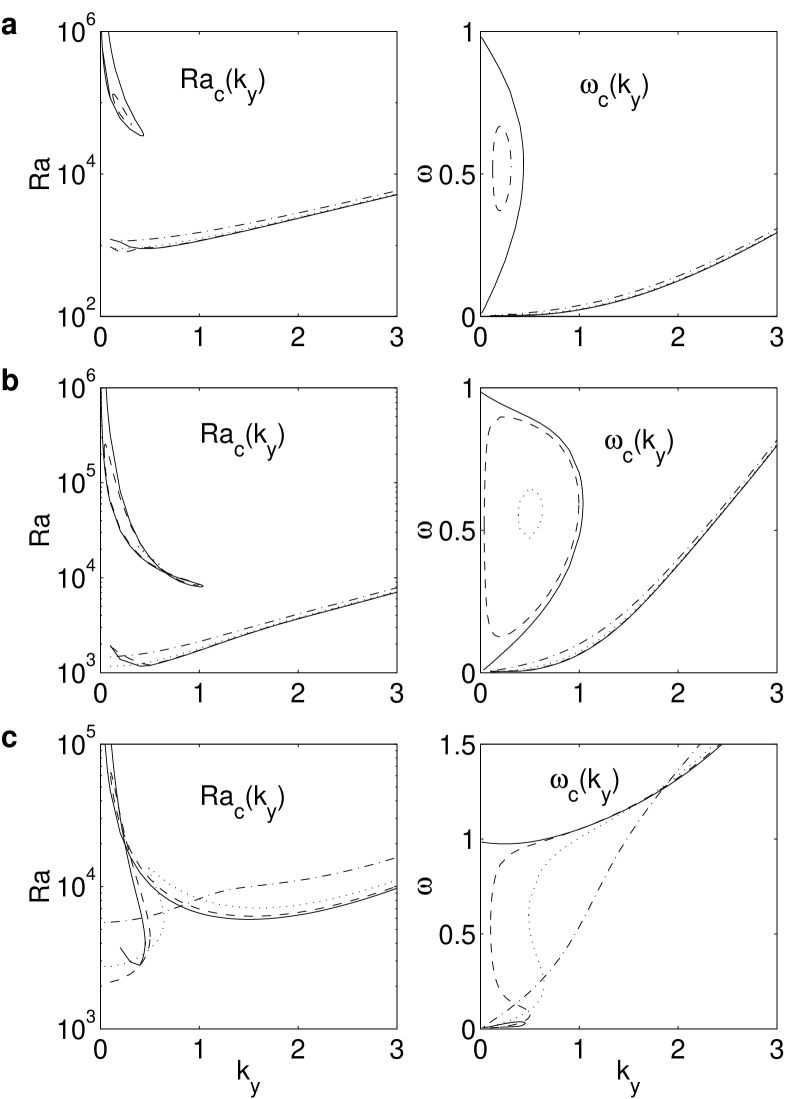
Figure 20: Viscous fluid and no-slip slot boundaries; $\eta=\chi=0$. Curves of the marginal linear stability to 3D ($k_{z}\geq 0$) oscillatory disturbances for different $k_{z}$, $Ra_{c}(k_{y})$ and $\omega_{c}(k_{y})$; $\mu=1$, $Pr=6.7$, $Le=1$. The solid lines: $k_{z}=0$, the dashed lines: $k_{z}=0.2$ in (a) and (b) and $k_{z}=0.5$ in (c), the dotted lines: $k_{z}=0.5$ in (a) and (b) and $k_{z}=1$ in (c), the dash-dot lines: $k_{z}=1$ in (a) and (b) and $k_{z}=2$ in (c). (a) $\theta=1.75\pi/2$; (b) $\theta=1.5\pi/2$; (c) $\theta=1.25\pi/2$. The lowest-$\omega_{c}(k_{y})$ data near $k_{y}=0$ (where such stable data were numerically difficult to obtain) are not presented. Additional quantitative details are given in Table 2.

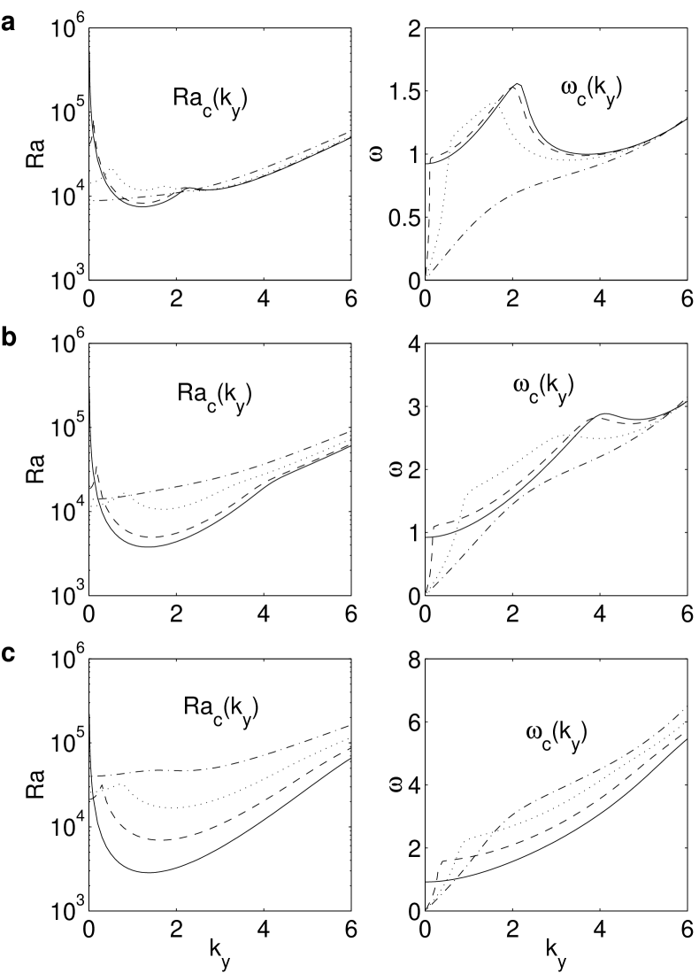
Figure 21: Viscous fluid and no-slip slot boundaries; $\eta=0$, $\chi=1$. Curves of the marginal linear stability to 3D ($k_{z}\geq 0$) oscillatory disturbances for different $k_{z}$, $Ra_{c}(k_{y})$ and $\omega_{c}(k_{y})$; $\mu=1$, $Pr=6.7$, $Le=1$. (a) $\theta=(1\pm 0.75)\pi/2$; (b) $\theta=(1\pm 0.5)\pi/2$; (c) $\theta=(1\pm 0.25)\pi/2$. The two values of $\theta$ are relevant in light of transformation (20). The solid lines: $k_{z}=0$; the dashed lines: (a) $k_{z}=0.5$, (b) $k_{z}=1$, (c) $k_{z}=2$; the dotted lines: (a) $k_{z}=1$, (b) $k_{z}=2$, (c) $k_{z}=3$; the dash-dot lines: (a) $k_{z}=2$, (b) $k_{z}=3$, (c) $k_{z}=4$. Additional quantitative details are given in Table 3.

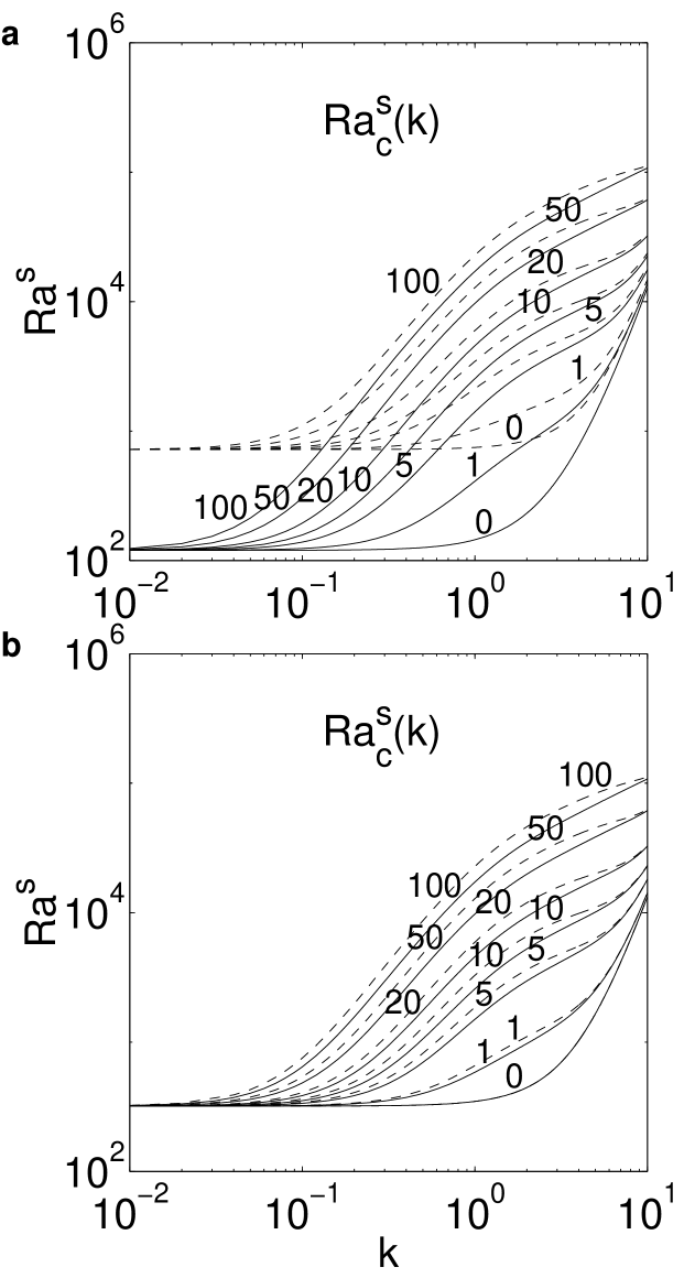
Figure 22: $\theta=\pi$. Viscous fluid; $\eta=\chi=0$. Curves of the marginal linear stability to steady disturbances, $Ra_{c}^{s}(k)$, for different $Ra$; $Le=1$. The numbers multiplied by $10^{3}$ give the values of $Ra$ for which the respective closest lines below them were computed. (a) the solid lines: $\gamma_{\pm}=0$, the dashed lines: $\gamma_{\pm}=1$; (b) the solid lines: $\gamma_{-}=0$ and $\gamma_{+}=1$, the dashed lines: $\gamma_{-}=1$ and $\gamma_{+}=0$. The most unstable wave numbers are described in Table 4.

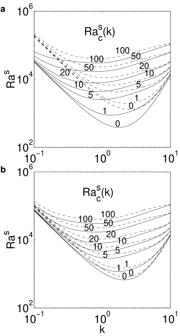
Figure 23: $\theta=\pi$. Viscous fluid; $\eta=\chi=1$. Curves of the marginal linear stability to steady disturbances, $Ra_{c}^{s}(k)$, for different $Ra$; $Le=1$. The numbers multiplied by $10^{3}$ give the values of $Ra$ for which the respective closest lines below them were computed. (a) the solid lines: $\gamma_{\pm}=0$, the dashed lines: $\gamma_{\pm}=1$; (b) the solid lines: $\gamma_{-}=0$ and $\gamma_{+}=1$, the dashed lines: $\gamma_{-}=1$ and $\gamma_{+}=0$. The most unstable wave numbers are described in Table 4.

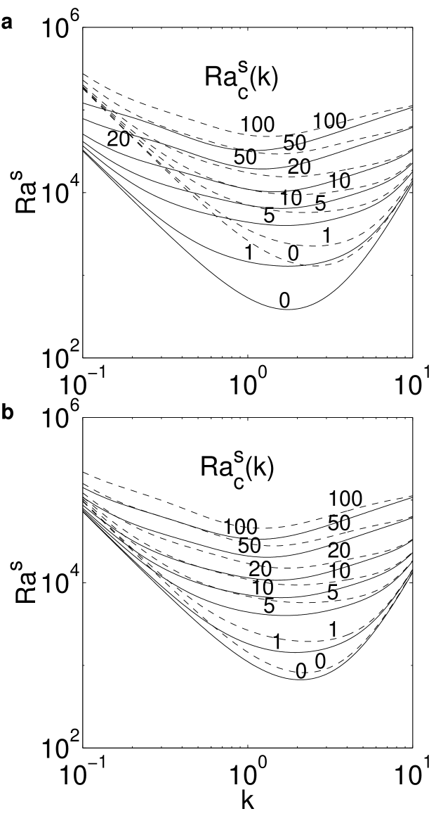
Figure 24: $\theta=\pi$. Viscous fluid; $\eta=0$, $\chi=1$. [These data also apply to $\theta=0$ if transformation (20) along with $Ra\mapsto Ra^{s}$, $Ra_{c}^{s}\mapsto Ra_{c}$, and $\gamma_{\pm}\mapsto\gamma_{\mp}$ are allowed for.] Curves of the marginal linear stability to steady disturbances, $Ra_{c}^{s}(k)$, for different $Ra$; $Le=1$. The numbers multiplied by $10^{3}$ give the values of $Ra$ for which the respective closest lines below them were computed. (a) the solid lines: $\gamma_{\pm}=0$, the dashed lines: $\gamma_{\pm}=1$; (b) the solid lines: $\gamma_{-}=0$ and $\gamma_{+}=1$, the dashed lines: $\gamma_{-}=1$ and $\gamma_{+}=0$. The most unstable wave numbers are described in Table 4.

Figure 25: $\theta=0$. Viscous fluid and no-slip slot boundaries; $\eta=\chi=1$. Schematic structures of the 2D steady flows with minimal along-slot period $\lambda=2$ for $\mu\in[0,1.5]$; $Pr=6.7$, $Le=1$. $\Phi$ is an abstract measure of the steady flows that distinguishes between different solutions, specifies the location of the singularities (limit points and symmetry-breaking bifurcations), and represents the flows arising from a symmetry-breaking bifurcation as a single branch. The background states are depicted by the horizontal lines with arrows (for $\mu=1.5$, this is the coordinate axis). The solid lines stand for the solutions being stable to the disturbances associated with the eigenvalues that give rise to the steady instability of the conduction state. The dashed lines represent the flows being unstable to either steady or both steady and oscillatory disturbances. The dotted lines stand for the solutions being unstable to oscillatory disturbances alone. Secondary bifurcations, if any, are not shown. $B$ is the symmetry-breaking bifurcation standing for the steady linear stability boundary for wave number $k=\pi$ ($\lambda=2$). Its criticality changes at $\mu$ just below $0.3$. $L$ is the limit point. $A1$ and $A2$ are the lower- and higher-amplitude branches associated with the limit point, respectively. H is a Hopf bifurcation. For $\mu=1$, it arises just below $Ra\approx 85040$ (Fig. 10).

Table 1: Inviscid fluid; $\eta=0$, $\chi=1$; $\mu=1$, $Le=1$. $k_{y}^{2l}(k_{z})$, $k_{y}^{2u}(k_{z})$, $k_{y}^{3l}(k_{z})$, and $k_{y}^{3u}(k_{z})$ are approximate values of wave number $k_{y}$ at which $Ra_{c}(k_{y})$ and $\omega_{c}(k_{y})$ are expected to decrease to zero for different $\theta$ and $k_{z}$. $k_{y}^{2l}(k_{z})$ and $k_{y}^{2u}(k_{z})$ originate at $k_{z}=0$, whereas $k_{y}^{3l}(k_{z})$ and $k_{y}^{3u}(k_{z})$ arise only at $k_{z}>0$. For $k_{z}\geq 0$, $q_{y}^{l}(k_{z})\equiv[{k_{y}^{2l}(0)}^{2}-k_{z}^{2}]^{1/2}$ and $q_{y}^{u}(k_{z})\equiv[{k_{y}^{2u}(0)}^{2}-k_{z}^{2}]^{1/2}$ are provided for comparison with $k_{y}^{2l}(k_{z})$ and $k_{y}^{2u}(k_{z})$, respectively. The two values of $\theta$ are relevant due to transformation (20).

$\theta$	$k_{z}$	$k_{y}^{3l}$	$k_{y}^{3u}$	$k_{y}^{2l}$	$k_{y}^{2u}$	$q_{y}^{l}$	$q_{y}^{u}$
	$0.0$	Not found	Not found	$0.3500$	$0.8954$	$0.3500$	$0.8954$
	$0.1$	$0.0109$	$0.0312$	$0.3189$	$0.8844$	$0.3354$	$0.8898$
	$0.15$	$0.0249$	$0.0840$	$0.2660$	$0.8704$	$0.3162$	$0.8827$
$(1\mp 0.85)\pi/2$	$0.2$	$0.0453$	Not found	Not found	$0.8496$		$0.8728$
	$0.3$	$0.1105$	Not found	Not found	$0.7847$		$0.8436$
	$0.4$	$0.2327$	Not found	Not found	$0.6622$		$0.8011$
	$0.5$	Not found	Not found	Not found	Not found
	$0.0$	Not found	Not found	$0.5959$	$1.4562$	$0.5959$	$1.4562$
	$0.1$	$0.0063$	$0.0169$	$0.5789$	$1.4495$	$0.5874$	$1.4528$
	$0.2$	$0.0254$	$0.0753$	$0.5206$	$1.4303$	$0.5613$	$1.4424$
	$0.25$	$0.0401$	$0.1322$	$0.4639$	$1.4154$	$0.5409$	$1.4346$
	$0.3$	$0.0585$	$0.2741$	$0.3221$	$1.3966$	$0.5149$	$1.4250$
$(1\mp 0.75)\pi/2$	$0.4$	$0.1079$	Not found	Not found	$1.3465$		$1.4001$
	$0.5$	$0.1780$	Not found	Not found	$1.2781$		$1.3677$
	$0.6$	$0.2784$	Not found	Not found	$1.1741$		$1.3268$
	$0.75$	$0.6027$	Not found	Not found	$0.8483$		$1.2482$
	$0.76$	$0.6910$	Not found	Not found	$0.7600$		$1.2421$
	$0.77$	Not found	Not found	Not found	Not found
	$0.0$	Not found	Not found	$1.3006$	$2.7783$	$1.3006$	$2.7783$
	$0.5$	$0.0665$	$0.2019$	$1.1006$	$2.7039$	$1.2007$	$2.7329$
	$0.6$	$0.0971$	$0.3266$	$0.9756$	$2.6697$	$1.1539$	$2.7127$
$(1\mp 0.5)\pi/2$	$0.7$	$0.1344$	Not found	Not found	$2.6284$		$2.6887$
	$1.0$	$0.2954$	Not found	Not found	$2.4523$		$2.5921$
	$1.5$	$0.9178$	Not found	Not found	$1.7937$		$2.3386$
	$1.55$	$1.0848$	Not found	Not found	$1.6222$		$2.3057$
	$1.6$	Not found	Not found	Not found	Not found

Table 1: (Continued)

$\theta$	$k_{z}$	$k_{y}^{3l}$	$k_{y}^{3u}$	$k_{y}^{2l}$	$k_{y}^{2u}$	$q_{y}^{l}$	$q_{y}^{u}$
	$0.0$	Not found	Not found	$2.0795$	$4.3196$	$2.0795$	$4.3196$
	$1.0$	$0.1136$	$0.3379$	$1.7081$	$4.1517$	$1.8233$	$4.2023$
	$1.3$	$0.2004$	$0.7769$	$1.2421$	$4.0289$	$1.6231$	$4.1193$
	$1.33$	$0.2108$	$0.9239$	$1.0932$	$4.0140$	$1.5986$	$4.1097$
$(1\mp 0.25)\pi/2$	$1.4$	$0.2365$	Not found	Not found	$3.9787$		$4.0864$
	$1.5$	$0.2767$	Not found	Not found	$3.9236$		$4.0508$
	$2.0$	$0.5583$	Not found	Not found	$3.5556$		$3.8287$
	$2.2$	$0.7264$	Not found	Not found	$3.3475$		$3.7174$
	$2.7$	$1.6070$	Not found	Not found	$2.3569$		$3.3718$
	$2.8$	Not found	Not found	Not found	Not found
	$0.0$	Not found	Not found	$2.3988$	$5.9121$	$2.3988$	$5.9121$
	$1.0$	$0.0429$	$0.1166$	$2.1658$	$5.8015$	$2.1804$	$5.8269$
	$1.5$	$0.1025$	$0.3052$	$1.8162$	$5.6620$	$1.8720$	$5.7186$
	$1.7$	$0.1356$	$0.4432$	$1.5889$	$5.5887$	$1.6924$	$5.6624$
	$1.9$	$0.1752$	$0.7245$	$1.2013$	$5.5035$	$1.4643$	$5.5985$
$(1\mp 0.1)\pi/2$	$1.93$	$0.1818$	$0.8369$	$1.0709$	$5.4891$	$1.4245$	$5.5882$
	$1.95$	$0.1862$	Not found	Not found	$5.4804$		$5.5813$
	$2.0$	$0.1977$	Not found	Not found	$5.4565$		$5.5635$
	$3.0$	$0.5673$	Not found	Not found	$4.7860$		$5.0944$
	$3.5$	$0.9303$	Not found	Not found	$4.2388$		$4.7648$
	$4.1$	$2.0274$	Not found	Not found	$2.9020$		$4.2595$
	$4.2$	Not found	Not found	Not found	Not found
	$0.0$	Not found	Not found	$2.4677$	$\infty$	$2.4677$	$\infty$
	$0.5$	Not found	Not found	$2.4165$	$\infty$	$2.4165$	$\infty$
$\pi/2$	$1.0$	Not found	Not found	$2.2560$	$\infty$	$2.2560$	$\infty$
	$1.5$	Not found	Not found	$1.9595$	$\infty$	$1.9595$	$\infty$
	$2.0$	Not found	Not found	$1.4455$	$\infty$	$1.4455$	$\infty$

Table 2: Viscous fluid and no-slip slot boundaries; $\eta=\chi=0$; $\mu=1$, $Pr=6.7$, $Le=1$. $k_{y}^{u}(k_{z})$ and $k_{y}^{l}(k_{z})$ are approximate locations of the limit points of the upper and lower branches, respectively, of $Ra_{c}(k_{y},k_{z})$ and $\omega_{c}(k_{y},k_{z})$ for different $k_{z}>0$ and such $\theta$ as the limit points are connected to intervals of the primary-instability boundary [Fig. 20(c)]. Sign $\approx$ implies that the accuracy with which the number was obtained is smaller than that of the other numbers, due to very small values of $\omega_{c}$ near such a limit point. For $\theta=(1+0.35)\pi/2$, the limit points vanish just below $k_{z}=1$.

$k_{z}$		$0.1$	$0.2$	$0.3$	$0.5$	$1$	$2$
$\theta=(1+0.35)\pi/2$	$k_{y}^{u}$	$0.0057$	$0.0230$	$0.0531$	$0.1620$	Not found	Not found
	$k_{y}^{l}$	$0.7656$	$0.7768$	$0.7953$	$0.8546$	Not found	Not found
$\theta=(1+0.25)\pi/2$	$k_{y}^{u}$	$0.0038$	$0.0154$	$0.0353$	$0.1031$	$0.4895$	Not found
	$k_{y}^{l}$	$\approx 0.4550$	$\approx 0.4603$	$0.4703$	$0.5023$	$0.6442$	Not found
$\theta=(1+0.15)\pi/2$	$k_{y}^{u}$	$0.0022$	$0.0089$	$0.0203$	$0.0581$	$0.2454$	Not found
	$k_{y}^{l}$	$\approx 0.2469$	$\approx 0.2520$	$0.2572$	$0.2740$	$0.3473$	Not found

Table 3: Viscous fluid and no-slip slot boundaries; $\eta=0$, $\chi=1$; $\mu=1$, $Pr=6.7$, $Le=1$. $k_{y}^{G}(k_{z})$ and $k_{y}^{\theta}(k_{z})$ are approximate values of wave number $k_{y}$ for different $k_{z}$ at a given $\theta$ where relatively abrupt changes in $\partial Ra_{c}/\partial k_{y}$ are distinguishable. (Such respective changes in $\partial\omega_{c}/\partial k_{y}$, in particular in Fig. 21, could be most pronounced at slightly shifted values of $k_{y}$.) $k_{y}^{\theta}(k_{z})$ originate at $k_{z}=0$, whereas $k_{y}^{G}(k_{z})$ arise only at $k_{z}>0$. For $k_{z}\geq 0$, $q_{y}^{\theta}(k_{z})\equiv[{k_{y}^{\theta}(0)}^{2}-k_{z}^{2}]^{1/2}$ are provided for comparison with $k_{y}^{\theta}(k_{z})$. For $\theta=(1\pm 0.5)\pi/2$, $k_{y}^{\theta}(k_{z})$ stands for the values of $k_{y}$ where the respective relatively abrupt change in $\partial\omega_{c}/\partial k_{y}$ takes place at a given $k_{z}$, since such a change in $\partial Ra_{c}/\partial k_{y}$ is then little distinguishable. The two values of $\theta$ are relevant due to transformation (20).

$\theta$	$k_{z}$	$k_{y}^{G}$	$k_{y}^{\theta}$	$q_{y}^{\theta}$
	$0.0$	Not found	$2.3$	$2.3$
$(1\pm 0.75)\pi/2$	$0.5$	$0.107$	$2.2$	$2.24$
	$1.0$	$0.5$	$1.7$	$2.07$
	$2.0$	Not found	Not found	$1.14$
	$0.0$	Not found	$4.15$	$4.15$
	$0.5$	$0.04$	$4.10$	$4.12$
$(1\pm 0.5)\pi/2$	$1.0$	$0.175$	$3.90$	$4.03$
	$2.0$	$0.8$	$3.20$	$3.64$
	$3.0$	Not found	Not found	$2.87$
	$0.0$	Not found	Not found
	$0.5$	$0.0175$	Not found
	$1.0$	$0.07$	Not found
$(1\pm 0.25)\pi/2$	$2.0$	$0.3$	Not found
	$3.0$	$0.7$	Not found
	$4.0$	$1.6$	Not found
	$5.0$	Not found	Not found

Table 4: $\theta=\pi$. Viscous fluid; $Le=1$. Approximate values of the most unstable wave number, $k_{c}$, and of the respective $Ra_{c}^{s}(k_{c})$ for the linear steady instability at the values of $Ra$ and $\gamma_{\pm}$ used for Figs. 22, 23, and 24. For $\eta=0$ and $\chi=1$, these data also apply to $\theta=0$ if transformation (20) along with $Ra\mapsto Ra^{s}$, $Ra_{c}^{s}\mapsto Ra_{c}$, and $\gamma_{\pm}\mapsto\gamma_{\mp}$ are allowed for.

$Ra$			$0$	$1000$	$5000$	$10000$	$20000$	$50000$	$100000$
	$\gamma_{\pm}=0$	$k_{c}$	$0$	$0$	$0$	$0$	$0$	$0$	$0$
$\eta=\chi=0$		$Ra_{c}^{s}(k_{c})$	$120$	$120$	$120$	$120$	$120$	$120$	$120$
[Fig. 22(a)]	$\gamma_{\pm}=1$	$k_{c}$	$0$	$0$	$0$	$0$	$0$	$0$	$0$
		$Ra_{c}^{s}(k_{c})$	$720$	$720$	$720$	$720$	$720$	$720$	$720$
	$\gamma_{-}=0$,	$k_{c}$	$0$	$0$	$0$	$0$	$0$	$0$	$0$
$\eta=\chi=0$	$\gamma_{+}=1$	$Ra_{c}^{s}(k_{c})$	$320$	$320$	$320$	$320$	$320$	$320$	$320$
[Fig. 22(b)]	$\gamma_{-}=1$,	$k_{c}$	$0$	$0$	$0$	$0$	$0$	$0$	$0$
	$\gamma_{+}=0$	$Ra_{c}^{s}(k_{c})$	$320$	$320$	$320$	$320$	$320$	$320$	$320$
	$\gamma_{\pm}=0$	$k_{c}$	$1.76$	$1.36$	$0.97$	$0.85$	$0.77$	$0.79$	$0.85$
$\eta=\chi=1$		$Ra_{c}^{s}(k_{c})$	$385$	$882$	$2539$	$4392$	$7825$	$17007$	$30186$
[Fig. 23(a)]	$\gamma_{\pm}=1$	$k_{c}$	$2.55$	$2.21$	$1.54$	$1.28$	$1.09$	$0.91$	$0.85$
		$Ra_{c}^{s}(k_{c})$	$1296$	$1980$	$4284$	$6744$	$11167$	$22973$	$40590$
	$\gamma_{-}=0$,	$k_{c}$	$2.09$	$1.71$	$1.22$	$1.04$	$0.91$	$0.82$	$0.83$
$\eta=\chi=1$	$\gamma_{+}=1$	$Ra_{c}^{s}(k_{c})$	$669$	$1183$	$2870$	$4704$	$8048$	$17024$	$30241$
[Fig. 23(b)]	$\gamma_{-}=1$,	$k_{c}$	$2.21$	$1.84$	$1.27$	$1.07$	$0.93$	$0.83$	$0.84$
	$\gamma_{+}=0$	$Ra_{c}^{s}(k_{c})$	$817$	$1482$	$3717$	$6159$	$10630$	$22706$	$40574$
	$\gamma_{\pm}=0$	$k_{c}$	$1.76$	$1.75$	$1.69$	$1.59$	$1.44$	$1.22$	$1.07$
$\eta=0$, $\chi=1$		$Ra_{c}^{s}(k_{c})$	$385$	$1289$	$4003$	$6437$	$10246$	$19327$	$32200$
[Fig. 24(a)]	$\gamma_{\pm}=1$	$k_{c}$	$2.55$	$2.51$	$2.20$	$1.96$	$1.76$	$1.51$	$1.32$
		$Ra_{c}^{s}(k_{c})$	$1296$	$2255$	$5745$	$9445$	$15500$	$29334$	$47784$
	$\gamma_{-}=0$,	$k_{c}$	$2.09$	$1.94$	$1.68$	$1.59$	$1.49$	$1.31$	$1.16$
$\eta=0$, $\chi=1$	$\gamma_{+}=1$	$Ra_{c}^{s}(k_{c})$	$669$	$1431$	$4008$	$6584$	$10718$	$20322$	$33526$
[Fig. 24(b)]	$\gamma_{-}=1$,	$k_{c}$	$2.21$	$2.35$	$2.20$	$1.96$	$1.72$	$1.43$	$1.23$
	$\gamma_{+}=0$	$Ra_{c}^{s}(k_{c})$	$817$	$1949$	$5733$	$9372$	$15004$	$27897$	$45606$

Table 5: $\theta=0$. Viscous fluid; $\lambda=2$, $Pr=6.7$, $Le=1$. Obtained from the numerical steady solutions of Eqs. (1)—(3), approximate values of $Ra$ characterizing limit point $L$ and symmetry-breaking bifurcation point $B$ (Fig. 25) for $\eta=\chi=1$ at $\gamma_{\pm}=1$ and such singularities for some $\eta=\chi<1$ at $\gamma_{\pm}=1$ and $\gamma_{\pm}=0$ in the range of $\mu\leq 1$.

$\mu$		$0.3$	$0.4$	$0.5$	$0.6$	$0.7$	$1$
$\eta=\chi=1$	$L$	$2726$	$3261$	$3872$	$4581$	$5417$	$9071$
$\gamma_{\pm}=1$	$B$	$2733$	$3419$	$4547$	$6694$	$11834$	$\infty$
$\eta=\chi\approx 0.64$	$L$	Not found	Not found	$3682$	$4855$	$6563$	$25107$
$\gamma_{\pm}=1$	$B$	$2299$	$2844$	$3716$	$5300$	$8800$	$\infty$
$\eta=\chi\approx 0.41$	$L$	Not found	Not found	Not found	$4983$	$7713$	$269057$
$\gamma_{\pm}=1$	$B$	$2194$	$2708$	$3524$	$4992$	$8184$	$\infty$
$\eta=\chi\approx 0.41$	$L$	Not found	Not found	$1616\div 1617$	$2274$	$3343$	$96701$
$\gamma_{\pm}=0$	$B$	$980$	$1223$	$1616\div 1617$	$2342$	$3938$	$\infty$

References

• [1] M.Β E.Β Stern, Tellus 12 (1960) 172–175.
• [2] G.Β Veronis, J. Mar. Res. 23 (1965) 1–17;
G.Β Veronis, J. Fluid Mech. 34 (1968) 315–336;
R.Β L.Β Sani, AIChE (Am. Inst. Chem. Eng.) J. 11 (1965) 971–980.
• [3] M.Β E.Β Stern, Deep-Sea Res. 14 (1967) 747–753.
• [4] J.Β S.Β Turner, Annu. Rev. Fluid Mech. 6 (1974) 37–54;
J.Β S.Β Turner, Annu. Rev. Fluid Mech. 17 (1985) 11–44.
• [5] R.Β W.Β Schmitt, Annu. Rev. Fluid Mech. 26 (1994) 255–285;
see also special issues of Prog. Oceanogr. 56 (2003) 381–570.
• [6] E.Β A.Β Spiegel, Annu. Rev. Astron. Astrophys. 10 (1972) 261–304;
D.Β W.Β Hughes, M.Β R.Β E.Β Proctor, Annu. Rev. Fluid Mech. 20 (1988) 187–223;
V.Β M.Β Canuto, Astrophys. J. 524 (1999) 311–340.
• [7] H.Β E.Β Huppert, R.Β S.Β J.Β Sparks, Annu. Rev. Earth Planet. Sci. 12 (1984) 11–37.
• [8] S.Β I.Β Braginsky, P.Β H.Β Roberts, Geophys. Astrophys. Fluid Dyn. 79 (1995) 1–97;
P.Β H.Β Roberts, G.Β A.Β Glatzmaier, Rev. Mod. Phys. 72 (2000) 1081–1123;
F.Β H.Β Busse, Geophys. Res. Lett. 29 (2002) 1105.
• [9] S.Β R.Β Coriell, R.Β F.Β Sekerka, PCH, PhysicoChem. Hydrodyn. 2 (1981) 281–293;
C.Β W.Β Lan, Chem. Eng. Sci. 59 (2004) 1437–1457.
• [10] H.Β A.Β Bethe, Rev. Mod. Phys. 62 (1990) 801–866;
A.Β Mezzacappa, Annu. Rev. Nucl. Part. Sci. 55 (2005) 467–515;
K.Β Kotake, K.Β Sato, K.Β Takahashi, Rep. Prog. Phys. 69 (2006) 971–1143;
A.Β Burrows, L.Β Dessart, C.Β D.Β Ott, E.Β Livne, Phys. Rep. 442 (2007) 23–37;
H.-Th.Β Janka, K.Β Langanke, A.Β Marek, G.Β Martinez-Pinedo, B.Β MΓΌller, Phys. Rep. 442 (2007) 38–74.
• [11] D.Β M.Β Mueth, J.Β C.Β Crocker, S.Β E.Β Esipov, D.Β G.Β Grier, Phys. Rev. Lett. 77 (1996) 578–581.
• [12] B.Β Martin, X.Β L.Β Wu, Phys. Rev. Lett. 80 (1998) 1892–1895.
• [13] S.Β Leibovich, J. Fluid Mech. 82 (1977) 561–581.
• [14] S.Β Leibovich, Annu. Rev. Fluid Mech. 15 (1983) 391–427;
S.Β A. Thorpe, Annu. Rev. Fluid Mech. 36 (2004) 55–79.
• [15] H.Β Stommel, Tellus 13 (1961) 224–230.
• [16] J.Β A.Β Whitehead, Annu. Rev. Fluid Mech. 27 (1995) 89–113;
J.Β A.Β Whitehead, J. Phys. Oceanogr. 39 (2009) 1231–1243.
• [17] C.Β Rooth, Prog. Oceanogr. 11 (1982) 131–149.
• [18] G.Β Walin, Palaeogeogr. Palaeoclimatol. Palaeoecol. 50 (1985) 323–332.
• [19] C.Β Quon, M.Β Ghil, J. Fluid Mech. 245 (1992) 449–483;
H.Β A.Β Dijkstra, M.Β J.Β Molemaker, J. Fluid Mech. 331 (1997) 169–198.
• [20] T.Β Kuhlbrodt, A.Β Griesel, M.Β Montoya, A.Β Levermann, M.Β Hofmann, S.Β Rahmstorf, Rev. Geophys. 45 (2007) RG2001.
• [21] M.Β Hofmann, S.Β Rahmstorf, Proc. Nat. Acad. Sci. USA 106 (2009) 20584–20589.
• [22] W.Β S.Β Broecker, D.Β M.Β Peteet, D.Β Rind, Nature 315 (1985) 21–26;
W.Β S.Β Broecker, G.Β H.Β Denton, Geochim. Cosmochim. Acta 53 (1989) 2465–2501;
W.Β S.Β Broecker, Oceanography 4 (1991) 79–89;
W.Β S.Β Broecker, Science 278 (1997) 1582–1588;
D.Β J.Β R.Β Thornalley, S.Β Barker, W.Β S.Β Broecker, H.Β Elderfield, I.Β N.Β McCave, Science 331 (2011) 202–205.
• [23] R.Β B.Β Alley, Annu. Rev. Earth Planet. Sci. 35 (2007) 241–272.
• [24] S.Β Manabe, R.Β J.Β Stouffer, J. Clim. 1 (1988) 841–866;
S.Β Manabe, R.Β J.Β Stouffer, Nature 378 (1995) 165–167;
S.Β Rahmstorf, Nature 419 (2002) 207–214;
P.Β U.Β Clark, N.Β G.Β Pisias, T.Β F.Β Stocker, A.Β J.Β Weaver, Nature 415 (2002) 863–869;
E.Β Bard, Phys. Today 55(12) (2002) 32–38.
• [25] R.Β P.Β Behringer, Rev. Mod. Phys. 57 (1985) 657–687.
• [26] M.Β C.Β Cross, P.Β C.Β Hohenberg, Rev. Mod. Phys. 65 (1993) 851–1112;
E.Β Bodenschatz, W.Β Pesch, G.Β Ahlers, Annu. Rev. Fluid Mech. 32 (2000) 709–778;
E.Β Knobloch, Nonlinearity 21 (2008) T45–T60.
• [27] P.Β Welander, Tellus, Ser. A 41 (1989) 66–72.
• [28] N.Β Tsitverblit, in: S. Meacham (Ed.), Double-Diffusive Processes, Woods Hole Oceanographic Institution, Technical Report No. WHOI-97-10, 1997, pp. 145–159.
• [29] N.Β Tsitverblit, Phys. Fluids 9 (1997) 2458–2460.
• [30] N.Β Tsitverblit, Phys. Fluids 11 (1999) 2516–2538.
• [31] N.Β Tsitverblit, Phys. Rev. E 62 (2000) R7591–R7594.
• [32] N.Β Tsitverblit, Ann. Phys. 322 (2007) 1727–1770.
• [33] L.Β K.Β Ingel, J. Exp. Theor. Phys. 102 (2006) 188–193;
L.Β K.Β Ingel, Dokl. Earth Sci. 408 (2006) 555–558.
• [34] S.Β A.Β Thorpe, P.Β K.Β Hutt, R.Β Soulsby, J. Fluid Mech. 38 (1969) 375–400;
J.Β E.Β Hart, J. Fluid Mech. 49 (1971) 279–288;
J.Β E.Β Hart, J. Fluid Mech. 59 (1973) 47–64;
S.Β Thangam, A.Β Zebib, C.Β F.Β Chen, J. Fluid Mech. 112 (1981) 151–160;
Y.Β Young, R.Β Rosner, Phys. Rev. E 57 (1998) 5554–5563;
O.Β S.Β Kerr, K.Β Y.Β Tang, J. Fluid Mech. 392 (1999) 213–232.
• [35] S.Β Xin, P.Β Le QuΓ©rΓ©, L.Β S.Β Tuckerman, Phys. Fluids 10 (1998) 850–858; see also the references therein.
• [36] S.Β Rosenblat, S.Β H.Β Davis, SIAM (Soc. Ind. Appl. Math.) J. Appl. Math. 37 (1979) 1–19.
• [37] N.Β Tsitverblit, Phys. Lett. A 329 (2004) 445–450.
• [38] H.Β R.Β Quinn, Phys. Today 56(2) (2003) 30–35;
F.Β Wilczek, Nature 433 (2005) 239–247.
• [39] J.Β L.Β Lebowitz, Phys. Today 46(9) (1993) 32–38;
J.Β L.Β Lebowitz, Physica A 194 (1993) 1–27;
J.Β L.Β Lebowitz, Rev. Mod. Phys. 71 (1999) S346–S357.
• [40] A.Β D.Β Sakharov, Sov. Phys. JETP 52 (1980) 349–351;
R.Β Peierls, Phys. Today 47(11) (1994) 115–115.
• [41] A.Β J.Β Weaver, C.Β M.Β Bitz, A.Β F.Β Fanning, M.Β M.Β Holland, Annu. Rev. Earth Planet. Sci. 27 (1999) 231–285.
• [42] G.Β I.Β Taylor, Phil. Trans. R. Soc. Ser. A 223 (1923) 289–343.
• [43] T.Β Mullin, J. Fluid Mech. 121 (1982) 207–218.
• [44] T.Β B.Β Benjamin, T.Β Mullin, J. Fluid Mech. 121 (1982) 219–230.
• [45] M.Β Golubitsky, I.Β Stewart, Arch. Ration. Mech. Anal. 87 (1985) 107–165;
J.Β D.Β Crawford, E.Β Knobloch, Annu. Rev. Fluid Mech. 23 (1991) 341–387.
• [46] A.Β A.Β Predtechensky, W.Β D.Β McCormick, J.Β B.Β Swift, Z.Β Noszticzius, H.Β L.Β Swinney, Phys. Rev. Lett. 72 (1994) 218–221;
A.Β A.Β Predtechensky, W.Β D.Β McCormick, J.Β B.Β Swift, A.Β G.Β Rossberg, H.Β L.Β Swinney, Phys. Fluids 6 (1994) 3923–3935.
• [47] A.Β Bergeon, K.Β Ghorayeb, A.Β Mojtabi, Phys. Fluids 11 (1999) 549–559;
G.Β Bardan, A.Β Bergeon, E.Β Knobloch, A.Β Mojtabi, Physica D 138 (2000) 91–113;
A.Β Bergeon, E.Β Knobloch, Phys. Fluids 14 (2002) 3233–3250;
A.Β Bergeon, E.Β Knobloch, Phys. Fluids 20 (2008) 034102;
A.Β Bergeon, E.Β Knobloch, Physica D 237 (2008) 1139–1150.
• [48] H.Β B.Β Keller, in: P.Β H.Β Rabinowitz (Ed.), Applications of Bifurcation Theory, Academic, New York, 1977, pp. 359–384.
• [49] D.Β A.Β Nield, J. Fluid Mech. 29 (1967) 545–558.
• [50] E.Β M.Β Sparrow, R.Β J.Β Goldstein, V.Β K.Β Jonsson, J. Fluid Mech. 18 (1964) 513–528;
D.Β T.Β J.Β Hurle, E.Β Jakeman, E.Β R.Β Pike, Proc. R. Soc. Ser. A 296 (1967) 469–475.
• [51] S.Β Leibovich, S.Β K.Β Lele, I.Β M.Β Moroz, J. Fluid Mech. 198 (1989) 471–511.
• [52] Lord Rayleigh, Phil. Mag. 32 (1916) 529–546;
W.Β H.Β Reid, D.Β L.Β Harris, Phys. Fluids 1 (1958) 102–110.
• [53] W.Β Barten, M.Β LΓΌcke, M.Β Kamps, R.Β Schmitz, Phys. Rev. E 51 (1995) 5636–5661.
• [54] A.Β E.Β Deane, E.Β Knobloch, J.Β Toomre, Phys. Rev. A 36 (1987) 2862–2869.
• [55] J.Β W.Β SandstrΓΆm, Ann. Hydrogr. Mar. Meteorol. 36 (1908) 6–23;
J.Β W.Β SandstrΓΆm, GΓΆteb. Kungl. Vetensk. Vitterh. Hand. 27 (1916) 1–48;
H.Β Jeffreys, Q. J. R. Meteorol. Soc. 51 (1925) 347–356.
• [56] C.Β Wunsch, R.Β Ferrari, Annu. Rev. Fluid Mech. 36 (2004) 281–314.
• [57] G.Β O.Β Hughes, R.Β W.Β Griffiths, Annu. Rev. Fluid Mech. 40 (2008) 185–208.
• [58] W.Β H.Β Munk, Deep-See Res. 13 (1966) 707–730;
W.Β Munk, C.Β Wunsch, Deep-Sea Res. 45 (1998) 1977–2010;
C.Β Garrett, L.Β St.Β Laurent, J. Oceanogr. 58 (2002) 11–24;
C.Β Garrett, E. Kunze, Annu. Rev. Fluid Mech. 39 (2007) 57–87.
Refer to caption