Abstract

In this paper, the problem of the minimal description of the structure of a vector function $f(x)$ over an $N$-dimensional interval is studied. Methods adaptively subdividing the original interval in smaller subintervals and evaluating $f(x)$ at only one point within each subinterval are considered. Two partition strategies traditionally used for solving this problem are analyzed. A new partition strategy based on an efficient technique developed for diagonal algorithms is proposed and studied.

Key Words: Partitioning, minimal description, one-point-based algorithms, global optimization.

1 Introduction and Analysis of Traditional Partition
Strategies

The problem of the minimal description of the behavior of a vector function

$$f(x)=(f_{1}(x),f_{2}(x),...,f_{r}(x)),\hskip 14.22636ptr\geq 1,$$ (1)

over a hyperinterval $D\subset\mathbb{R}^{N}$ can be stated in various ways under different assumptions regarding $f(x)$. The term ‘minimal description’ means that we want to obtain a knowledge about $f(x)$ by evaluating it in a minimal number of trial points $x\in D$. The problem has a number of important applications in numerous fields of mathematics such as optimization, number theory, numerical integration, geometric partitioning, and structural description (see Ref. 1 for discussion and references). Usually, in real-life applications, the operation of evaluating $f(x)$ requires much time and to obtain an acceptable solution of the minimal description problem it is necessary to execute a high number of such evaluations.

Numerous iterative processes proposed in literature (see Refs. 1–19, etc.) for solving this problem can be distinguished in dependence on the way they combine the following four features: (i) the strategy used for partition of the region $D$; (ii) the way to choose an element (or elements) for the next partition; (iii) the number of points $f(x)$ should be evaluated at the new subregions obtained after partition; (iv) the location of these points within each of the new subregions.

Let us determine the place of our study with respect to the features (i)–(iv). First, one-point-based, diagonal, simplicial, etc. algorithms (see, for example, Refs. 1–19) can be distinguished relatively to the feature (i) and (iii). one-point-based algorithms subsequently subdivide the region $D$ in smaller hyperintervals and evaluate $f(x)$ at one point within each sub-interval (the terms ‘cell’ and ‘box’ will be also used). Diagonal methods do the same but evaluate $f(x)$ at two vertices of each box. Simplicial algorithms partition the region in simplexes and evaluate the objective vector function at all their vertices. The current state-of-art in the field (see Refs. 2, 7, 11, 15) does not allow us to say which of the approaches is worse or better for a given class of functions.

This paper deals with popular one-point-based algorithms that have been extensively studied theoretically (mainly from the feature (ii) point of view (see Refs. 6, 8, 11, 12, 14, 15, etc.)). They have also been successfully applied to solve numerous real-life problems. For example, interval analysis methods use mainly this strategy in their work (see, for instance, Refs. 7, 10, 11). Another important example of their usage comes from the DIRECT optimization method introduced in Ref. 12 that also has been employed in a number of industrial applications (see Refs. 5, 17, 18 ).

Peculiarity of this paper consists of the following: it does not discusses the feature (ii). In contrast, its goal is to show (as it has been already done for the diagonal methods in Ref. 1) that partition strategies themselves, independently of the feature (ii), can influence significantly the number of function evaluations made by an algorithm. Thus, we concentrate our attention on the features (i) and (iv) in the framework of one-point-based algorithms.

Let us analyze two partition strategies traditionally used in the one-point-based algorithms. In the first of them, the region $D$ is subdivided in a number of sub-intervals and $f(x)$ is evaluated at an internal (very often central) point of each of the new sub-boxes. Then a new sub-cell of $D$ is chosen for partitioning and the process is repeated. This simple and widely used strategy has the following drawback. If $f(x)$ has been evaluated at a point $x^{i}$ within an interval $D(i)$ only the interval $D(i)$ uses the information obtained from evaluation of $f(x^{i})$.

The second traditional partition strategy overcomes this difficulty. An internal point (indicated in Fig. 1a by the number $1$) is chosen within the region $D$ that is subdivided in $2^{N}$ sub-boxes by the hyperplanes orthogonal to coordinate axes and passing through this point. In this strategy, the information obtained at every point is used by $2^{N}$ intervals. Unfortunately, such a huge number of sub-boxes creates problems during managing the description information when the dimension of the problem, $N$, increases. This strategy has also the second problem illustrated in Fig. 1b.

Suppose that the interval shown by grey color in Fig. 1a has been chosen for the next subdivision. It can be seen from Fig. 1b that the partition executed within this interval at the point $2$ creates redundancy in the following sense. The one-point-based algorithms use only one point for description of $f(x)$ over each interval $D(i)$. In spite of this, the interval shown by grey color has two points where $f(x)$ has been evaluated. One of them is redundant. In general, usage of this partition strategy leads to the following result describing the level of the obtained redundancy.

Proposition 1.1 Every partition made by using the second strategy leads to creation of one or two sub-cells having $f(x)$ evaluated at two vertices.

Proof: Let us consider the situation where one interval having $f(x)$ evaluated at two vertices is generated. This happens when an interval having $f(x)$ evaluated at one of its vertices (see Fig. 1a) is subdivided. Two intervals having redundant points are generated when an interval with $f(x)$ evaluated at two of its vertices (see the interval shown in grey in Fig. 1b) is subdivided.  

The analysis given above shows that a desirable partition strategy should not generate too many sub-cells during every partition and should be able to avoid redundant evaluations of the vector function $f(x)$ giving in the same moment to several intervals a possibility to use the information obtained from every single evaluation of $f(x)$.

2 Strategy

In this paper, a new partition strategy that can be used by one-point-based algorithms is proposed. It is based on an efficient partition strategy introduced recently in Ref. 1 for solving the minimal description problem in the framework of diagonal algorithms (see Ref. 15). These methods evaluate the vector function $f(x)$ at two vertices $a(i)$ and $b(i)$ of each sub-box $D(i)$ where

$$D(i)=[a(i),b(i)]=\{x:a(i)\leq x\leq b(i)\}.$$

A high practical efficiency of the new strategy applied for solving global optimization problems has been shown in Ref. 13.

In order to proceed, let us describe this partition strategy developed for diagonal algorithms. A cell $D(t)=[a(t),b(t)]$ chosen for subdivision among $L(k)$ cells existing during an iteration $k$ is split into three equal sub-intervals by two hyperplanes orthogonal to the longest edge parallel to the $i$th coordinate axis and passing through the points

$$u=(a_{1}(t),a_{2}(t),\ldots,a_{i-1}(t),a_{i}(t)+2(b_{i}(t)-a_{i}(t))/3,a_{i+1}(t),\ldots,a_{N}(t)),$$ (2)

$$v=(b_{1}(t),b_{2}(t),\ldots,b_{i-1}(t),b_{i}(t)+2(a_{i}(t)-b_{i}(t))/3,b_{i+1}(t),\ldots,b_{N}(t)).$$ (3)

The cell $D(t)$ is substituted by the new cells $D(t(k)),D(L(k)+1),$ and $D(L(k)+2)$ determined by their vertices

$$\hskip 28.45274pt\begin{array}[]{llr}a(t(k))=a(L(k)+2)=u,&b(t(k))=b(L(k)+1)=v,&\hskip 56.9055pt(4a)\\ a(L(k)+1)=a(t(k)),&b(L(k)+1)=v,&\hskip 56.9055pt(4b)\\ a(L(k)+2)=u,&b(L(k)+2)=b(t(k)).&\hskip 56.9055pt(4c)\end{array}$$

The function $f(x)$ is (eventually) evaluated at the points $u$ and $v$.

It has been shown in Ref. 1 that this strategy generates regular trial meshes in such a way that every cell has exactly two vertices where the function $f(x)$ is evaluated. The introduced regularization allows to establish links between sub-cells generated during different iterations eliminating in this way possibility of the redundant trials generation and storage of the related information.

While using this strategy it becomes possible (see Ref. 1) to reestablish information about vicinity of the cells generated during different iterations and, as the result, to eliminate redundant storage of the points $a(j),b(j)$ and results of evaluations of the function $f(x)$ at these points. Particularly, it is shown that every vertex where $f(x)$ is evaluated can belong to different (up to $2^{N}$) cells. When we split an interval $D(t)$, we calculate the coordinates of the vertices corresponding to the three new sub-cells. Particularly, we are interested in the vertices $u$ and $v$, the only two vertices for the three cells from (4) where the function $f(x)$ should be evaluated.

Instead of an immediate evaluation of the values $f(u)$ and $f(v)$, we verify the existence of these in the data base because $f(u)$ and/or $f(v)$ could have been already evaluated during previous iterations. It is important to mention that two numerations (one for the boxes and another for the vertices where the function $f(x)$ has been evaluated) have been developed theoretically in Ref. 1 and successfully applied practically in Ref. 13. These numerations allow us to calculate the addresses of $u$ and $v$ in the data base of the vertices from the number of the box $D(t)$ providing so a direct fast access to the values $f(u)$ and $f(v)$.

If both of them have been already evaluated, we simply read these values from the data base. If only one of them has been evaluated, we read this value and create a new element in the data base for the absent (say $u$) point, evaluate $f(u)$ and record it in the element created. In the last case – both values are absent – these operations are executed for both points.

Thus, the description information is evaluated at every vertex only once and then we simply read it up to $2^{N}$ times instead of evaluating $f(x)$ and saving the result of this evaluation and coordinates of the $2^{N}$ trial points $2^{N}$ times.

Surprisingly, this strategy developed for the diagonal methods can be successfully applied for the one-point-based algorithms too. Instead of evaluating $f(x)$ at two vertices, $u$ and $v$, it is proposed to do this initially for the vertex $a$ of the region $D$ and then at the vertex $u$ during every splitting (the point $v$ is used just for partitioning goals). Then, the operation of the verification whether the function $f(x)$ has been already evaluated at this point is made by using the fast procedure developed in Ref. 1.

In order to illustrate the new strategy, let us consider an example presented in Fig. 2. The first evaluation of the function $f(x)$ is executed at the vertex $a$ (see Fig. 2a). The second evaluation is made at the point $2$ being the point $u$ from (2). It can be seen from this figure that we have three sub-cells having exactly one vertex where $f(x)$ has been evaluated. Suppose that the interval shown in grey in Fig. 2a has been chosen for the next splitting (see Fig. 2b). The only evaluation made at the point $3$ gives us three new intervals. It seems that the interval chosen for the next partitioning (and shown again in grey) has a redundant point, i.e., the point $3$. In reality, this point is not a redundant one but is kept in the data base and can be used in the future. Fig. 2c shows that the fourth point coincides with the point $3$, thus, no evaluations are made, the description information is read from the data base and we obtain three new smaller intervals gratis. Finally, Fig. 2d illustrates situation after eleven iterations. It can be seen from this figure that $21$ intervals have been generated and the function has been evaluated at seven points only.

3 Conclusions

In this paper, the problem of the minimal description of a function $f(x)$ over a hyperinterval $D$ has been considered in the framework of the one-point-based algorithms. An analysis of the traditional partitioning strategies used by these methods has been made. It has been shown that the meshes of the trial points generated by these strategies can generate redundant points and intervals. Such a redundancy may lead to a significant increase of information to be stored in the computer memory and to the slowing down the description procedure.

A new partition strategy has been introduced to overcome these difficulties. It generates regular trial meshes successfully responding to the requirements of the minimal description. During every partitioning it generates three intervals independently on the problem dimension. Since every point where the function has been evaluated can belong up to $2^{N}$ intervals and it is possible to establish links between sub-cells generated during different iterations, the function is evaluated at every trial point only once and then the result of this evaluation is simply read from the data base many times. As a rule, this fact very often allows to obtain new partitions without any evaluation of the function.

References

1. Sergeyev, Ya. D., An Efficient Strategy for Adaptive Partition of N-Dimensional Intervals in the Framework of Diagonal Algorithms, Journal of Optimization Theory and Applications, Vol. 107, pp. 145–168, 2000.

2. Agarwal, P. K., Geometric Partitioning and Its Applications, DIMACS Series in Discrete Mathematics and Theoretical Computer Science, Edited by J. E. Goodman, R. Pollack, and J. O’Rourke, Vol. 6, pp. 1–37, 1991.

3. Baritompa, W. P., and Viitanen, S., PMB-Parallel Multidimensional Bisection, Report 101, Department of Mathematics and Statistics, University of Canterbury, Christchurch, New Zealand, 1993.

4. Breiman, L., and Cutler, A., A Deterministic Algorithm for Global Optimization, Mathematical Programming, Vol. 58, pp. 179–199, 1993.

5. Cox, S. E., Haftka, R. T., Baker, C., Grossman, B., Mason, W. H., and Watson, L. T., A Comparison of Global Optimization Methods for the Design of a High-Speed Civil Transport, Journal of Global Optimization, Vol. 21, pp. 415–433, 2001.

6. Csendes, T. and Ratz, D., Subdivision Direction Selection in Interval Methods for Global Optimization, SIAM Journal of Numerical Analysis, Vol. 34, pp. 922–938, 1997.

7. Floudas, C., and Pardalos, P. M., State of the Art in Global Optimization: Computational Methods and Applications, Kluwer Academic Publishers, Dordrecht, the Netherlands, 1995.

8. Galperin, E. A., The Cubic Algorithm, Journal of Mathematical Analysis and Applications, Vol. 112, pp. 635–640, 1985.

9. Gergel, V.P., A Global Optimization Algorithm for Multivariate Functions with Lipschitzian First Derivatives, Journal of Global Optimization, Vol. 10, pp. 257-281, 1997.

10. Hansen, E. R., Global Optimization Using Interval Analysis, Marcel Dekker, New York, NY, 1992.

11. Horst, R., and Pardalos, P. M., Handbook of Global Optimization, Kluwer Academic Publishers, Dordrecht, the Netherlands, 1995.

12. Jones, D. R., Perttunen, C. D., and Stuckman, B. E., Lipschitzian Optimization without the Lipschitz Constant, Journal of Optimization Theory and Applications, Vol. 79, pp. 157–181, 1993.

13. Kvasov, D. E., and Sergeyev, Ya. D., Multidimensional Global Optimization Algorithm Based on Adaptive Diagonal Curves, Computational Mathematics and Mathematical Physics, Vol. 43, pp. 40–56, 2003.

14. Meewella, C. C., and Mayne, D. Q., Efficient Domain Partitioning Algorithms for Global Optimization of Rational and Lipschitz Continuous Functions, Journal of Optimization Theory and Applications, Vol. 61, pp. 247–270, 1989.

15. Pintér, J. D., Global Optimization in Action, Kluwer Academic Publishers, Dordrecht, the Netherlands, 1996.

16. Strongin, R. G., and Sergeyev, Ya. D., Global Optimization with Non-Convex Constraints: Sequential and Parallel Algorithms, Kluwer Academic Publishers, Dordrecht, the Netherlands, 2000.

17. Verstak, A., He, J., Watson, L. T, Ramakrishnan, N., Shaffer, C. A., Rappaport, T. S., Anderson, C. R., Bae, K., Jiang, J., and Tranter, W. H., S4W: Globally Optimized Design of Wireless Communication Systems, Proceedings of the Next Generation Software Workshop: 16th International Parallel and Distributed Processing Symposium, IEEE Computer Society Press, Fort Lauderdale, Florida, pp. 173–180, 2002.

18. Watson, L. T., and Baker, C. A., A Fully-Distributed Parallel Global Search Algorithm, Engineering Computations, Vol. 18, pp. 155–169, 2001.

19. Wood, G. R., The Bisection Method in Higher Dimensions, Mathematical Programming, Vol. 55, pp. 319–337, 1992.

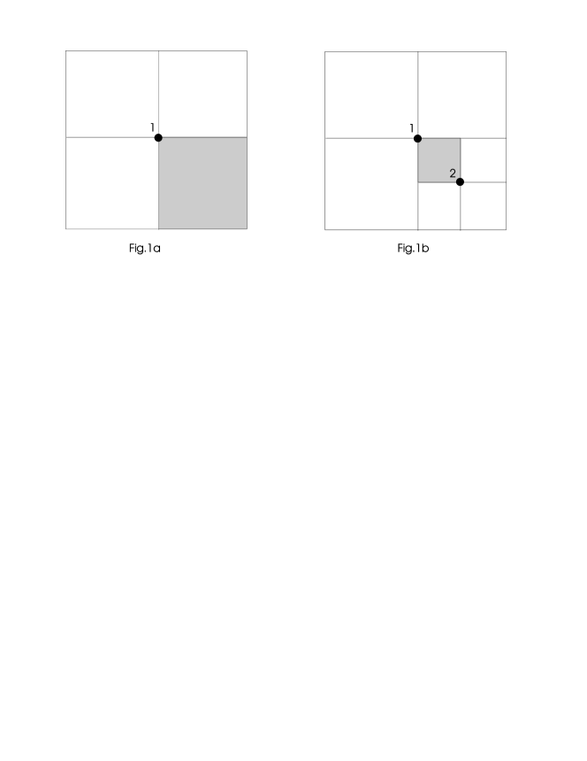
Figure 1:

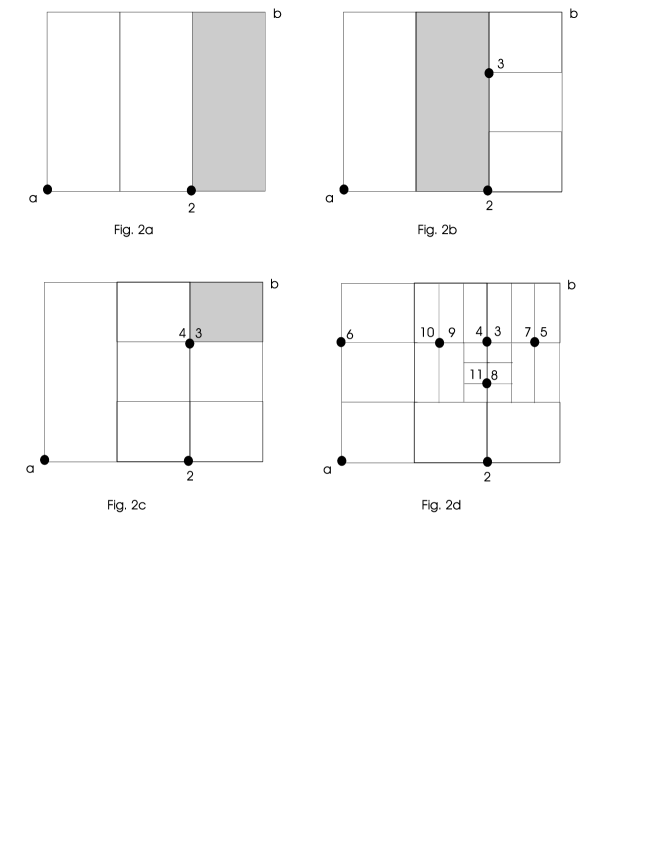
Figure 2: