Poles, the only true resonant-state signals, are extracted from a worldwide collection of partial wave amplitudes using only one, well controlled pole-extraction method

Abstract

Each and every energy dependent partial–wave analysis is parameterizing the pole positions in a procedure defined by the way how the continuous energy dependence is implemented. These pole positions are, henceforth, inherently model dependent. To reduce this model dependence, we use only one, coupled–channel, unitary, fully analytic method based on the isobar approximation to extract the pole positions from the each available member of the worldwide collection of partial wave amplitudes which are understood as nothing more but a good energy dependent representation of genuine experimental numbers assembled in a form of partial–wave data. In that way, the model dependence related to the different assumptions on the analytic form of the partial–wave amplitudes is avoided, and the true confidence limit for the existence of a particular resonant state, at least in one model, is established. The way how the method works, and first results are demonstrated for the S₁₁ partial wave.

I Introduction

When resonances are associated with the eigenstates of the complete Hamiltonian for which there are only asymptotically outgoing waves, their identification with scattering theory poles is unquestionable. This statement is in details elucidated in ref. Dal70 . Consequently, in order to get the full information about physical systems and resonant states under observation, we must be entirely focused onto analyzing and interpreting the scattering matrix singularities of the Mandelstam analytic function Man58 obtained from experiments. While the value of the scattering amplitude on the positive energy cut defines the physical amplitude in the s or u channel depending whether we approach the physical axes from above or below, the simple poles which are situated on the physical axes in a subthreshold region are related to the bound states. As it is believed that there is no fundamental difference between a bound state and a resonance, other than the matter of stability, when simple poles of the coupled channel amplitude occur on unphysical sheets in the complex energy plane, they are to be associated with resonant states Mar70 .

The fact that we are trying to extract the value of a quantity lying in the complex energy plane while performing experiments only on the physical axes, is the essence of all problems, and origin of many misunderstandings occurring in the literature. Namely, each pole is not only squatting in an experimentally inapproachable domain, but is simultaneously governing each and every process between all allowed few body channels. However, we usually measure observables only in one channel at a time. If the single-channel observables are measured, we obtain the single-channel scattering amplitude, and we only get the pole positions in one channel. Nevertheless, due to the Mandelstam hypothesis, these poles are affecting all channels, so we have to treat them all and not just the measured one. Consequently, the underlying theory which is to be used to find the scattering matrix amplitude must be a coupled-channel one, and of course analytic and unitary. And this is not the end. Once we have found the coupled-channel scattering matrix amplitude, we have to find and quantify all its poles. Unfortunately, this is not a simple task, so each partial wave analyses, even in a multi-channel case, has its own way of parameterizing this inaccessible quantity. The result is that the model dependencies are introduced.

This brings us to various ways how the complex energy plane poles are up to the present moment parameterized in the literature. First attempts are done with single-channel partial wave amplitudes, and the oldest and most frequently met way is the concept of Breit-Wigner parameters.

The initial attempts to use the Breit-Wigner function with constant parameters to represent the scattering matrix amplitudes on the physical axes immediately revealed the fact that this function is too simple. More terms were needed. One had to introduce the energy dependent background, and one had to do it in a unitary way. Unfortunately, for quite some time it has been known, but not commonly accepted, that a unitary addition of background terms influences the peak position of the scattering matrix absolute value on the real axes in spite of the fact that the pole position is not changed. Peak position is an interplay of Breit-Wigner parameters and background terms. And the peak position is the quantity which is usually extracted from experiments. Consequently, when Breit-Wigner parameters defined in such a manner are chosen to represent the pole position, they must be background dependent, and the only case when the Breit-Wigner parameters do exactly correspond to the pole position is when we have accidently guessed the correct form of the energy dependent background. If the background is wrong, Breit-Wigner parameters are not the pole parameters, but something else. And that is the reason why Breit-Wigner terms in general are not the pole positions, and are inherently model dependent.

There are basically two ways to account for the background contributions. The first one, to unitary add energy dependent background terms to the constant-parameter Breit-Wigner function, is described afore. The second one is to allow the Breit-Wigner parameters to become energy dependent. That is predominantly done by modeling the Breit-Wigner width Arndt1 ; Manley1 ; Manley2 ; Cutcosky1 ; Bat1 ; TPVrana .

There is a number of ways to introduce energy dependent Breit-Wigner width. In ref. Arndt1 energy dependent width is a part of resonant term of theoretical function which is associated with the T-matrix near the resonance. In refs. Manley1 ; Manley2 energy dependent width is related to the resonant part of the S-matrix. In a method proposed in ref Cutcosky1 and applied in refs. Bat1 ; TPVrana width is deffined from the function consisting of a background term and Breit-Wigner shape term.

One well known method for treating the nearby channel openings is the Flatté formula. The Flatté’s method, introduced in 1976 Fla76 , is recognizing the fact that the partial-wave T-matrix feels the presence of new channel openings, and it is taking it into account effectively. Flatté proposes to modify the traditional Breit-Wigner form by assuming that the width with becomes proportional to the phase space. The amplitude poles are then again represented as the singularities of the modified Breit-Wigner function.

The fact that the Breit-Wigner terms in general are not the pole positions, and are inherently model dependent, was timidly mentioned by several authors (see for instance ref. Pole_vs_BW ). That was first strongly pointed out by Höhler in refs. KH80 ; PDG1998 , where the definition of “local Breit-Wigner fit” and the concept of “searching for the pole position” using speed plot technique were introduced. Höhler clearly distinguished between Breit-Wigner parameters (which should in the absence of a better way be obtained by locally fitting partial wave amplitudes with a Breit-Wigner function plus some background terms) and pole parameters which should be obtained, as he recommended , by the speed plot technique. He has always been pointing out that Breit-Wigner parameters are model dependent, and he continuously objected to compare them directly. His last warning was published not so long ago PDG2000 . However, due to unclear historical reasons, the practice of direct comparing Breit-Wigner parameters coming from different origin continued in Particle Data Group (PDG) compilations. Breit-Wigner parameters, extracted with different background parameterizations are still directly compared PDG2010 , averages are made and error analysis is performed neglecting the fact that they may be in fact completely differently defined parameters. This practice should be abolished.

There is a long history of efforts to avoid the concept of Breit-Wigner parameters, and to look directly for the genuine pole positions.

The first, and most frequently met method, is the speed-plot technique introduced by Höhler KH80 for the single channel scattering amplitudes. It is based on the idea already mentioned in ref. Mar70 that the pole position should be found by expanding the scattering amplitude in the vicinity of the pole, and the speed-plot technique is recommending to retain the first term only. This method is in principle acceptable if we are dealing with isolated poles far away from any nearby thresholds, but my fail otherwise. There is a number of cases where the methods can not be applied at all, and the best example was inability to use it to obtain the well known S₁₁(1535) resonance. The limitations of the method have been discussed by Ceci et al. Ceci08 where it has been shown that speed-plot technique is only the $N$=1 term of a more general but demanding “regularization” method based on finding the N-th derivative of the scattering amplitude, and using it in a local, three-parameter fit to the partial wave data Mainz2010 .

In the early fifties the time delay technique is introduced into scattering theory by several authors Eisenbud1 ; Wigner1 ; Wigner2 ; Bohm , in a way that they obtained expression for the time delay in a collision. Time delay, or in another words the time lapse between asymptotic states, can be directly related with phase shift of the T matrix. For further details on interrelation between speed plot and time delay see ref. Suzuki1 .

The N/D method is a technique in which the dispersion relations are used to construct the amplitudes in the physical region using the knowledge of the left-hand cut singularities. The idea is to represent the partial-wave amplitude as a ratio of two functions. The numerator is represented with a function N(s) which is analytic in the s-plane only on the left-hand cut, and the function D(s) that is analytic on the right-hand cut only. The poles of the scattering amplitude are identified with the zeroes of the D(s), and the problem of extra zeroes is often difficult to be solved. The method has been introduced a long time ago by Chew60 , and since then it has been mostly used in meson physics, typically for cases when the knowledge about the left-hand cut is available Olle99 ; Ani06 .

All enlisted methods are good for the pole search within certain approximations, but yet we have to point out that the proper procedure to look for the scattering matrix poles is the full analytic continuation of scattering matrix amplitudes into the complex energy plane within a given model.

In coupled-channel calculations the importance of the pole-search has recently been fully recognized. Some groups have offered more or less detailed concepts of their analytic continuation procedures Arn04 ; EBAC , while others have reported that the complexity of the analytic continuation of all Feynman amplitudes of their model is beyond their reach Feu98 . Therefore, they had to rely on speed-plot technique entirely. In most cases, the analytic continuation procedure is rather cumbersome.

The VPI/GWU collaboration clearly distinguishes the difference between Breit-Wigner parameters and pole positions, and states that ”Poles and zeros have been found by continuing into the complex energy plane”. Unfortunately, they fail to provide any details of their procedure. The EBAC collaboration also makes an analytic extrapolation of their amplitudes, and has recently presented a more detailed elaboration of their procedures EBAC . Other groups have extracted their pole positions using single-channel techniques such as speed-plot and time delay Che03 ; Che07 ; Feu98 ; Giessen . Recognizing the importance of a direct analytic extrapolation, Dubna-Mainz-Taipei collaboration has recently performed the full analytic continuation, and in ref. Mainz2010 offered the reliable pole positions of their model.

In spite of all these efforts, the question of systematic uncertainties still remains unanswered, because each model has its own, particular analytic form. So we wonder how stable, with respect to the analytic continuation procedure, these pole positions actually are.

In order to get a reliable answer to this questions, we have decided to use only one method to extract pole positions from all published partial waves analyses, and compare the results. And we have chosen the T-matrix Carnagie-Melon-Berkeley (CMB) model. In other words, we take all sets of partial-wave amplitudes, treat them as nothing else but a good, energy dependent representations of all analyzed experimental data, and extract the poles which are required by the CMB method. In this manner, all errors due to different analytic continuations of different models are avoided, and the only remaining error is the precision of CMB method itself. We shall also compare the obtained poles with the poles of each individual publication, and draw certain conclusions about features of individual methods as well.

The general idea of this article is to recommend the possibility how to, in a maximally model independent way, simultaneously find all scattering matrix poles from the world-wide collection of partial wave amplitudes. We present the way of eliminating most systematic errors in analytic extrapolation by using only one, well defined procedure to extract pole positions for published partial wave amplitudes, understanding them as nothing more but a very confident energy dependent representation of all experimental data.

To avoid congesting the reader with unnecessary information, we in this paper in details illustrate how this method works for the S₁₁ partial wave only. We show that N(1535) and N(1650) S₁₁ resonant states are unambiguously seen in all analyzed PWA data, while the performed pole-search procedure strongly suggest the existence of at least one more pole position in the vicinity of 1800 MeV. Therefore, all published PWA are consistent with the new S₁₁(1846) state seen in photo-production channel Che03 ; Yan03 . We demonstrate that the existence of fourth S₁₁ state around 2100 Mev is not excluded by any PWA, and is actually favored for the hadronic Dubna-Mainz-Taipei amplitudes Che03 ; Che07 . We compare the obtained results with the results published in literature, and make a final conclusion on the actual position of partial wave poles.

However, the issue also arises how strongly the recommended pole-extraction procedure (CMB model) depends upon its own the model assumptions. Namely, CMB model has a number of assumptions, and it is very important to know how stable the pole positions are if CMB model choices are strongly modified. We have tested this problem extensively, and for the answer to this question we refer the reader to a parallel publication submitted to this journal Hedim2010 .

II Formalism

The CMB model is isobar, coupled-channel, analytic, and unitary model, where the T matrix in a given channel is assumed to be a sum over the contributions from a number of intermediate particles (resonance and background contributions). The coupling of the channel asymptotic states to these intermediate particles determines the imaginary part of the channel function, and is represented effectively with a separable function. The real part of the channel function is calculated by the dispersion relation technique, thus ensuring analyticity. Besides the known resonance contributions, the background contributions are included via additional terms with poles below the $\pi$N threshold. Due to the clear analytic and separable structure of the model, finding the pole positions in CMB model is trimmed down to the generalization of the dispersion integral for the channel propagator from real axes to the full complex energy plane, and this is a very well defined procedure. In practice, we instead use a very stable, and numerically much faster analytic continuation method based on the Pietarienen expansion Pietarinen in order to extrapolate the real valued channel propagator into the complex energy plane.

II.1 Formulae

Our current partial-wave analysis Bat98 is based on the manifestly unitary, multichannel CMB approach of ref. Cut79 . The most prominent property of this approach is analyticity of partial waves with respect to Mandelstam $s$ variable. In every discussion of partial-wave poles, analyticity plays a crucial role since the poles are situated in a complex plane, away from physical region, and our measuring abilities are restricted to the real energy axis only. To gain any knowledge about the nature of partial-wave singularities would be impossible if partial waves were not analytic. Therefore, the ability to calculate pole positions is not just a benefit of the CMB model’s analyticity but also a necessity for resonance extraction. In this approach, the resonance itself is considered to exist if there is an associated partial-wave pole in the “unphysical” sheet.

We use the multichannel $T$ matrix related to the scattering matrix $S$ as:

$$S_{ab}(s)=\delta_{ab}+2\,i\,T_{ab}(s),$$ (1)

where $\delta_{ab}$ is Kronecker delta symbol. The T-matrix matrix element is in the CMB model given as:

$$T_{ab}^{JL}(s)=\sum_{i,j=1}^{N^{JL}}f_{a}^{JL}(s)\sqrt{\rho_{a}(s)}\gamma_{ai}^{JL}G_{ij}^{JL}(s)\gamma_{jb}^{JL}\sqrt{\rho_{b}(s)}f_{b}^{JL}(s)$$

where $a(b)$ represents the outgoing (incoming) channel. In our analyses we use $a,b=\pi N,\eta N,\pi^{2}N$. The initial and final channel $b(a)$ couple through intermediate particles labeled $i$ and $j$. The factors $\gamma_{ia}$ are energy-independent parameters occurring graphically at the vertex between channel $a$ and intermediate particle $i$ and are determined by fitting procedure. Also occurring at each initial or final vertex is form factor $f_{a}^{JL}(s)$

$$f_{a}^{JL}(s)=\left(\frac{q_{a}}{Q_{1a}+\sqrt{Q_{2a}^{2}+q_{a}^{2}}}\right)^{L},$$ (2)

and phase-space factor $\rho_{a}(s)$

$$\rho_{a}(s)=\frac{q_{a}(s)}{\sqrt{s}},$$ (3)

where $s=W^{2}$ is a Mandelstam variable, and $q_{a}(s)$ is the meson momentum for any of the three channels given as

$$q_{a}(s)=\frac{\sqrt{(s-(m+m_{a})^{2})(s-(m-m_{a})^{2})}}{2\sqrt{s}}.$$ (4)

Furthermore, $L$ is the angular momentum in channel $a$, and $Q_{1a}$, $Q_{2a}$ are constants. The factor $f_{a}^{JL}(s)$ provides appropriate threshold behavior on the right-hand cut, and also produces a left-hand branch cut in the $s$ plane. Parameters $Q_{1a}$ and $Q_{2a}$ are chosen to determine the branch point and strength of the left-hand branch cut. In our analyses they have been taken to be the same, and are fixed to the mass of the channel meson $a$.

$G_{ij}^{JL}$ is a dressed propagator for partial wave $JL$ and particles $i$ and $j$, and may be written in terms of a diagonal bare propagator $G_{ij}^{0JL}$ and a self-energy matrix $\Sigma_{kl}^{JL}$ using Dyson equation

$$G_{ij}^{JL}(s) = G_{ij}^{0JL}(s)+\sum_{k,l=1}^{N^{JL}}G_{ik}^{0JL}(s)\Sigma_{kl}^{JL}(s)G_{ij}^{JL}(s).$$ (5)

The bare propagator

$$G_{ij}^{0JL}(s)=\frac{e_{i}\delta_{ij}}{s_{i}-s}$$ (6)

has a pole at the real value $s_{i}$. The sign $e_{i}=\pm 1$ must be chosen to be positive for poles above the elastic threshold which correspond to resonance.

The nonresonant background is described by a meromorphic function, in most of the cases consisting of two terms of the form (6) with pole positions below $\pi N$ threshold. For that case, the signs of the terms are opposite. The positive sign correspond to the repulsive and the negative sign to the attractive potential. In principle the number of poles can be increased arbitrarily (see the next subsection on background representation), but in reality the number is never larger than three.

$\Sigma_{kl}^{JL}$ is the self-energy term for the particle propagator

$$\Sigma_{kl}^{JL}(s)=\sum_{a}\gamma_{ka}^{JL}\cdot\Phi_{a}^{JL}(s)\cdot\gamma_{la}^{JL}$$ (7)

The $\Phi_{a}^{JL}(s)$ are called “channel propagators”. They are constructed in an approximation that threats each channel as containing only two particles. We require that $T_{ab}^{JL}$ have, in all channels, correct unitarity and analyticity properties consistent with a quasi-two-body approximation.

The imaginary part of $\Phi_{a}^{JL}(s)$ is the effective phase-space factor for channel $a$:

$$\mathrm{Im}\ \Phi_{a}^{JL}(s)=[f_{a}^{JL}(s)]^{2}\rho_{a}(s).$$ (8)

The channel propagator is evaluated on the real axes only

$$\mathrm{Im}\,\Phi(x)=\frac{\left[q(x)\right]^{2L+1}}{\sqrt{x}\,\left\{Q_{1}+\sqrt{Q_{2}^{2}+\left[q(x)\right]^{2}}\right\}^{2L}},\vspace*{0.1cm}$$ (9)

where by $x$ we stress the fact that values are on the real axes. The real part of $\Phi_{a}^{JL}(x)$ is calculated using a subtracted dispersion relation

$$\mathrm{Re}\,\Phi(x)=\frac{x-x_{a}}{\pi}\,\,\mathrm{P}\int_{x_{a}}^{\infty}\frac{\mathrm{Im}\,\Phi(x^{\prime})\,dx^{\prime}}{(x^{\prime}-x)(x^{\prime}-x_{a})}.$$ (10)

where $x_{a}=(m+m_{a})^{2}$. For better understanding, the structure of the channel-intermediate particle form factor is given in Fig. 1.

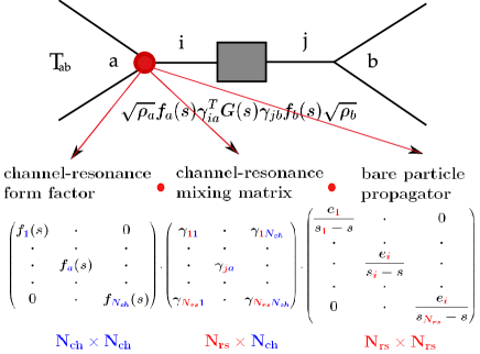
Figure 1: Parameterization of channel-intermediate particle vertex in CMB model.

We give a matrix form of the final T matrix as defined in Eq. (II.1):

$$\hat{T}(s)=\sqrt{Im\hat{\Phi}(s)}\cdot\hat{\gamma}^{\rm T}\cdot\frac{\hat{G}_{0}(s)}{I-\left[\hat{\gamma}\cdot\hat{\Phi}(s)\cdot\hat{\gamma}{\rm{}^{T}}\right]\cdot\hat{G}_{0}(s)}\cdot\hat{\gamma}\cdot\sqrt{Im\hat{\Phi}(s)}$$ (11)

II.2 General idea

In this paper we propose to use a method based on coupled-channel formalism, apply it to all partial wave data and partial wave amplitudes available “on the market”, and simultaneously analyze the underlying analytic structure. We have decided to use only one model to extract pole positions from all published partial waves analyses in order to evade the model assumptions of each approach, and compare the results on the same footing. And we have chosen the T-matrix Carnagie-Melon-Berkeley (CMB) model. In other words, we take all sets of partial-wave amplitudes, accept them as nothing else but good representations of all analyzed experimental data, and extract the poles which are required by the CMB method. In this manner, all errors due to different analytic continuations of different models are avoided, and the only remaining error is the precision of CMB method itself (see ref. Hedim2010 ). Of course, we shall compare the obtained poles with the poles of each individual publication, and draw certain conclusions about features of individual methods as well.

II.3 Data base

We start with a collection of data in which one part is fully available in the literature KH80 ; Arn04 ; GWUWEB , and numeric values for the second part are provided by the authors (private communication refs. Giessen ; Diaz07 ; Dur08 ; Che07 ; Juelich ).

We have analyzed the following PWA amplitudes:

1. Karlsruhe-Helsinki (KH80) KH80 - $\pi$N elastic;
   As the influence of inelastic channels is in KH80 formalism introduced through forward and fixed cms scattering dispersion relations, KH80 does not offer any inelastic channel amplitudes to be fitted. However, as we know that inelastic channels are extremely important in CMB formalism to ensure the stability of solutions (see following chapter and ref. Ceci06 ), we have decided to constrain elastic KH80 amplitudes with $\pi$N $\rightarrow\eta$N WI08 amplitudes which fairly correctly depict the world agreement of the $\eta$N channel amplitudes at lower energies - see Fig. 3.

2. VPI/GWU - $\pi$N elastic and $\pi$N $\rightarrow\eta$N;
   We have used single energy solutions (GWU-SES) GWUWEB , and energy dependent solutions (WI08) Arn04 ; GWUWEB .

3. Giessen Giessen - $\pi$N elastic and $\pi$N $\rightarrow\eta$N

4. EBAC - We have used two sets of PW solutions. Single-channel fit solution ($\pi$N elastic fitted) — EBAC07 Diaz07 , and two channel fit solution ($\pi$N elastic and $\pi$N $\rightarrow\eta$N fitted) — EBAC08 Dur08 with the $\pi$N $\rightarrow\eta$N normalization adjusted in accordance with M. Döring and B. Diaz Duering2009 . with M. Döring and B. Diaz Duering2009

5. Jülich Juelich - $\pi$N elastic and $\pi$N $\rightarrow\eta$N

6. Dubna-Mainz-Taipei (DMT) Che03 ; Che07 - $\pi$N elastic and $\pi$N $\rightarrow\eta$N

II.4 Fitting procedure

We have used three channel CMB formalism with $\pi$N and $\eta$N physical channels, and the third, effective two body channel to account for unitarity. We start with a minimal number of bare poles, and increase their number as long as the quality of the fit, measured by the lowest reduced $\chi^{2}$ value, could not be improved. In addition, a visual resemblance of the fitting curve to the data set in totality was used as a rule of thumb; i.e., we rejected those solutions that had a tendency to accommodate for the rapidly varying data points, regardless of the $\chi^{2}$ value. When the optimal number of poles is reached, we claim that we have found all partial wave pole solutions given by the chosen data set. As our criteria (minimal reduced $\chi^{2}$ value and visual resemblance) are not extremely rigid, we have to differentiate between the two categories of poles: those which are seen with almost complete certainty, and those which are only consistent with the chosen set of data. The poles whose addition significantly improve the reduced $\chi^{2}$ value fall into the first category, those which improve the reduced $\chi^{2}$ value only marginally fall into the second one. It is interesting to note that in the latter case a number of almost equivalent, indistinguishable solutions for the questionable pole may be found.

III Results and Discussion

The intention of this article is to use only one method, Zagreb realization of CMB model, to extract pole positions from a world collection of partial wave data and partial wave amplitudes. As a test case, we do it for the S₁₁ partial wave only. We use three channel model, with two measured channels $\pi$N, $\eta$N, and the third channel $\pi^{2}$N, which effectively represents all other inelastic channels, and “takes care of ” unitarity.

We extract pole positions from all available PWA and make a comprehensive analyses. We analyze the number of poles needed for a given partial wave, we discuss the importance of inelastic channels.

III.1 Methodology

The main feature of CMB multi-resonance, multi-channel model is a good control over determining the number of bare poles, and deducing the importance of number of fitted channels.

Importance of inelastic channels

The elastic $\pi$N scattering channel is the best measured and the most confident channel, so in all cases it is the pillar of the obtained partial wave amplitudes. Most of the information about the energy dependent structure of all solutions is coming from this channel, and it is expected that corrections are coming from other channels. Therefore, it is carrying the heaviest weight for obtaining final results.

At this point we are bound to address one specific point in more details.

In ref. Ceci06 we have discussed the continuum ambiguity problem in coupled-channel formalisms. Namely, once the inelastic channels are opened, it turns out that the differential cross sections themselves are not sufficient to determine the scattering amplitude. Let us illustrate why. If differential cross section $d\sigma/d\Omega$ is given by $|F|^{2}$, then the new function F̃ $=e^{i\Phi}F$ gives exactly the same cross section. It should be remarked that this phase uncertainty has nothing to do with the non-observable phase of wave functions in quantum mechanics. The asymptotic wave functions at large distances from the scattering center may be written as $\Psi(x)\approx e^{i\cdot k\cdot x}+F(\theta)\frac{e^{i\cdot r\cdot}}{r}$, $r\rightarrow\infty$, so the phase of scattering amplitude is the relative phase of the incident and scattered wave. This phase has observable consequences in situations where multiple scattering occurs, and the continuum ambiguity is created. In the elastic region, the unitarity relates real and imaginary parts of each partial wave, and the consequence is a constraint which effectively removes this ”continuum” ambiguity, and leaves potentially only a discreet one. The partial wave must lie on the unitary circle. However, as soon as the inelastic threshold opens, unitarity provides only an inequality: $|1+2\ i\ F_{l}|^{2}\leq 1\Longrightarrow{\rm ImF}_{l}=|F_{l}|^{2}+I_{l}$, where $I_{l}=\frac{1}{4}(1-e^{-\,4\,{\rm Im}\,\delta_{l}})$. Therefore, each partial wave must lie upon or inside its unitary circle, and not on it. A whole family of functions $\Phi$, of limited magnitude but of infinite variety of functional forms which satisfy the required conditions, does exist. However, in spite that they contain a continuum infinity of points, they are limited in extent. Thus, the islands of ambiguity are created.

In ref. Ceci06 we have shown that including inelastic channels into the analysis is a natural way for eliminating continuum ambiguities. We have concluded that, by fitting only elastic channel, some of the resonant states which dominantly couple to inelastic channels might remain unrevealed, and we had to fit as many channels as possible. In the present paper we apply the following strategy: we shall first fit elastic channel only, and show the poles we reveal. Then, we shall repeat the fit by fitting two channel processes, $\pi$N elastic and $\pi$N $\rightarrow\eta$N data when available, and see how the number of poles, and their quantitative values change.

The problem we are facing is the low quality input for the $\eta$N channel, because $\pi$N $\rightarrow\eta$N partial waves are in principle not well known. Anyway, as a final result, we have to accept the solution for which both channels are reasonably well fitted despite the low quality of the $\eta$N channel data.


Determining the optimal number of poles

In CMB formalism the number of poles is a starting parameter. That in practice means that when fitting, we start with a minimal set of poles: one resonant and two for the background. Then we increase the number of resonant poles until the satisfactory fit is achieved, i.e., until the quality of the fit, measured by the reduced $\chi^{2}$ value, could not be improved. In addition, a visual resemblance of the fitting curve to the data set as a whole is used as a rule of thumb: we reject all those solutions which have a tendency to accommodate for the rapidly varying data points regardless of the $\chi^{2}$ value.

In such a way we estimate the number of bare poles needed by our model, what in most cases corresponds to the number of resonant states. Observe that this is not so for dynamic resonances, i.e., for the dressed resonant states which do not have a corresponding bare pole. Therefore, what we compare is not the number of bare poles, but the number of dressed ones. (For a more extensive discussion on dynamic resonant states in Zagreb CMB model see ref. Ceci08 .)

III.2 Fits

We first fit $\pi$N elastic channel only. In accordance with the afore considerations, we first want to determine which resonances are we well determined only by this channel, and later on we want to see how much the inclusion of $\eta$N channel will modify the obtained result.

III.2.1 $\pi$N elastic channel only

We show the result of the fit in Table 1. The quality of the fit is shown in Fig. 2.

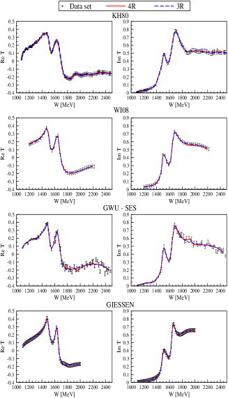
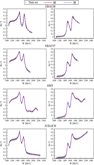
Figure 2: Agreement of 3R and 4R CMB curves with “world input” for single-channel fit.

Table 1: “World collection” of poles for the single-channel fit, three and four resonant case.

	Fitted	Number	Bare poles				Dressed poles
ANALYSES	channel	of	$\mathrm{W_{s_{1}}}$	$\mathrm{W_{s_{2}}}$	$\mathrm{W_{s_{3}}}$	$\mathrm{W_{s_{4}}}$	$\begin{pmatrix}\mathrm{ReW}\\ \mathrm{-2ImW}\end{pmatrix}$	$\begin{pmatrix}\mathrm{ReW}\\ \mathrm{-2ImW}\end{pmatrix}$	$\begin{pmatrix}\mathrm{ReW}\\ \mathrm{-2ImW}\end{pmatrix}$	$\begin{pmatrix}\mathrm{ReW}\\ \mathrm{-2ImW}\end{pmatrix}$	$\chi_{R}^{2}$
		resonances		$\mathrm{MeV}$				$\mathrm{MeV}$
KH80	$\pi N\rightarrow\pi N$	3	1516	1638	1880	-	$\begin{pmatrix}1513\\ 71\end{pmatrix}$	$\begin{pmatrix}1661\\ 148\end{pmatrix}$	$\begin{pmatrix}1903\\ 90\end{pmatrix}$	-	0.209
		4	1488	1656	1713	2266	$\begin{pmatrix}1513\\ 113\end{pmatrix}$	$\begin{pmatrix}1670\\ 194\end{pmatrix}$	$\begin{pmatrix}1833\\ 703\end{pmatrix}$	$\begin{pmatrix}2263\\ 138\end{pmatrix}$	0.206
WI08	$\pi N\rightarrow\pi N$	3	1481	1657	3767	-	$\begin{pmatrix}1492\\ 89\end{pmatrix}$	$\begin{pmatrix}1646\\ 95\end{pmatrix}$	$\begin{pmatrix}2684\\ 822\end{pmatrix}$	-	0.043
		4	1513	1624	1686	2517	$\begin{pmatrix}1495\\ 105\end{pmatrix}$	$\begin{pmatrix}1647\\ 81\end{pmatrix}$	$\begin{pmatrix}1658\\ 255\end{pmatrix}$	$\begin{pmatrix}2396\\ 139\end{pmatrix}$	0.012
GWU-SES	$\pi N\rightarrow\pi N$	3	1514	1645	2919	-	$\begin{pmatrix}1500\\ 106\end{pmatrix}$	$\begin{pmatrix}1646\\ 119\end{pmatrix}$	$\begin{pmatrix}2598\\ 210\end{pmatrix}$	-	2.252
		4	1517	1650	1928	3768	$\begin{pmatrix}1505\\ 97\end{pmatrix}$	$\begin{pmatrix}1651\\ 119\end{pmatrix}$	$\begin{pmatrix}1944\\ 74\end{pmatrix}$	$\begin{pmatrix}2633\\ 345\end{pmatrix}$	2.116
GIESSEN	$\pi N\rightarrow\pi N$	3	1464	1616	1731	-	$\begin{pmatrix}1484\\ 82\end{pmatrix}$	$\begin{pmatrix}1641\\ 65\end{pmatrix}$	$\begin{pmatrix}1861\\ 811\end{pmatrix}$	-	0.062
		4	1474	1635	1718	2674	$\begin{pmatrix}1482\\ 82\end{pmatrix}$	$\begin{pmatrix}1642\\ 65\end{pmatrix}$	$\begin{pmatrix}1851\\ 456\end{pmatrix}$	$\begin{pmatrix}2249\\ 287\end{pmatrix}$	0.061
JUELICH	$\pi N\rightarrow\pi N$	3	1518	1656	2177	-	$\begin{pmatrix}1528\\ 95\end{pmatrix}$	$\begin{pmatrix}1653\\ 110\end{pmatrix}$	$\begin{pmatrix}2335\\ 372\end{pmatrix}$	-	0.046
		4	1511	1636	1719	2241	$\begin{pmatrix}1516\\ 121\end{pmatrix}$	$\begin{pmatrix}1654\\ 118\end{pmatrix}$	$\begin{pmatrix}1665\\ 411\end{pmatrix}$	$\begin{pmatrix}2335\\ 403\end{pmatrix}$	0.018
EBAC07	$\pi N\rightarrow\pi N$	3	1466	1641	2518	-	$\begin{pmatrix}1498\\ 123\end{pmatrix}$	$\begin{pmatrix}1641\\ 89\end{pmatrix}$	$\begin{pmatrix}2215\\ 767\end{pmatrix}$	-	0.028
		4	1483	1643	1702	2237	$\begin{pmatrix}1502\\ 139\end{pmatrix}$	$\begin{pmatrix}1638\\ 81\end{pmatrix}$	$\begin{pmatrix}1700\\ 408\end{pmatrix}$	$\begin{pmatrix}1862\\ 691\end{pmatrix}$	0.012
EBAC08	$\pi N\rightarrow\pi N$	3	1515	1673	1826	-	$\begin{pmatrix}1483\\ 123\end{pmatrix}$	$\begin{pmatrix}1662\\ 80\end{pmatrix}$	$\begin{pmatrix}1873\\ 219\end{pmatrix}$	-	0.029
		4	1512	1667	1980	3784	$\begin{pmatrix}1492\\ 114\end{pmatrix}$	$\begin{pmatrix}1661\\ 81\end{pmatrix}$	$\begin{pmatrix}1804\\ 1113\end{pmatrix}$	$\begin{pmatrix}2189\\ 637\end{pmatrix}$	0.027
DMT	$\pi N\rightarrow\pi N$	3	1495	1643	2047	-	$\begin{pmatrix}1486\\ 81\end{pmatrix}$	$\begin{pmatrix}1640\\ 103\end{pmatrix}$	$\begin{pmatrix}2080\\ 100\end{pmatrix}$	-	0.246
		4	1507	1647	1850	2100	$\begin{pmatrix}1508\\ 139\end{pmatrix}$	$\begin{pmatrix}1643\\ 134\end{pmatrix}$	$\begin{pmatrix}1892\\ 203\end{pmatrix}$	$\begin{pmatrix}2100\\ 212\end{pmatrix}$	0.083
Averages		3					$\begin{pmatrix}1498(16)\\ 96(20)\end{pmatrix}$	$\begin{pmatrix}1649(9)\\ 101(25)\end{pmatrix}$	$\begin{pmatrix}2194(324)\\ 424(324)\end{pmatrix}$	-
		4					$\begin{pmatrix}1502(12)\\ 114(20)\end{pmatrix}$	$\begin{pmatrix}1651(11)\\ 109(42)\end{pmatrix}$	$\begin{pmatrix}1793(108)\\ 453(325)\end{pmatrix}$	$\begin{pmatrix}2253(224)\\ 356(212)\end{pmatrix}$

III.2.2 $\pi$N elastic and $\pi$N $\rightarrow\eta$N data

As we have already mentioned, $\pi$N $\rightarrow\eta$N data are rather old and vague, so the corresponding partial waves are poorly determined. Anyway, each analyzed PWA solution of our “world collection”, with the exception of KH80 does offer some results for that channel, and we have consistently used it in the two channels fit. The only exception, KH80 amplitudes, do not have a corresponding $\eta$N channel. We have been tempted to omit KH80 amplitudes from the coupled-channel analysis, but due to its extremely good analytical constraints, we have decided to keep it in some form. Instead of KH80 $\eta$N channel, we have used the WI08 VPI/GWU solution believing that the S₁₁ $\eta$N channel amplitudes are confidently well known in the energy range s $\leq$ 3 GeV² ($T_{lab}\leq 800$ MeV), and in that range the WI08 VPI/GWU solution is a good numeric representation of a “world collection average”.

We show the result of the fit in Table 2. The quality of the fit is shown in Fig. 3.

Table 2: “World collection” of poles for the two channels fit, three and four resonant case.

ANALYSIS		Number	Bare poles				Dressed poles
(Fitted channels)		of	$\mathrm{W_{s_{1}}}$	$\mathrm{W_{s_{2}}}$	$\mathrm{W_{s_{3}}}$	$\mathrm{W_{s_{4}}}$	$\begin{pmatrix}\mathrm{ReW}\\ \mathrm{-2ImW}\end{pmatrix}$	$\begin{pmatrix}\mathrm{ReW}\\ \mathrm{-2ImW}\end{pmatrix}$	$\begin{pmatrix}\mathrm{ReW}\\ \mathrm{-2ImW}\end{pmatrix}$	$\begin{pmatrix}\mathrm{ReW}\\ \mathrm{-2ImW}\end{pmatrix}$	$\chi_{R}^{2}$
		resonances		$\mathrm{MeV}$				$\mathrm{MeV}$
KH80	WI08	3	1517	1637	1865	-	$\begin{pmatrix}1511\\ 113\end{pmatrix}$	$\begin{pmatrix}1670\\ 163\end{pmatrix}$	$\begin{pmatrix}1923\\ 328\end{pmatrix}$	-	0.391
($\pi N\rightarrow\pi N$)	($\pi N\rightarrow\eta N$)	4	1504	1610	1751	2045	$\begin{pmatrix}1492\\ 122\end{pmatrix}$	$\begin{pmatrix}1650\\ 163\end{pmatrix}$	$\begin{pmatrix}1892\\ 235\end{pmatrix}$	$\begin{pmatrix}1951\\ 555\end{pmatrix}$	0.307
WI08		3	1514	1626	1722	-	$\begin{pmatrix}1499\\ 114\end{pmatrix}$	$\begin{pmatrix}1652\\ 102\end{pmatrix}$	$\begin{pmatrix}1718\\ 449\end{pmatrix}$	-	0.127
($\pi N\rightarrow\pi N$)	($\pi N\rightarrow\eta N$)	4	1513	1630	1701	2611	$\begin{pmatrix}1495\\ 113\end{pmatrix}$	$\begin{pmatrix}1651\\ 87\end{pmatrix}$	$\begin{pmatrix}1697\\ 204\end{pmatrix}$	$\begin{pmatrix}2422\\ 241\end{pmatrix}$	0.031
GWU-SES	WI08	3	1519	1662	3190	-	$\begin{pmatrix}1503\\ 172\end{pmatrix}$	$\begin{pmatrix}1642\\ 127\end{pmatrix}$	$\begin{pmatrix}2618\\ 270\end{pmatrix}$	-	2.451
($\pi N\rightarrow\pi N$)	($\pi N\rightarrow\eta N$)	4	1512	1643	1743	2827	$\begin{pmatrix}1503\\ 97\end{pmatrix}$	$\begin{pmatrix}1659\\ 111\end{pmatrix}$	$\begin{pmatrix}1756\\ 210\end{pmatrix}$	$\begin{pmatrix}2569\\ 173\end{pmatrix}$	2.011
GIESSEN		3	1515	1636	1720	-	$\begin{pmatrix}1472\\ 176\end{pmatrix}$	$\begin{pmatrix}1650\\ 81\end{pmatrix}$	$\begin{pmatrix}1692\\ 191\end{pmatrix}$	-	0.437
($\pi N\rightarrow\pi N$)	($\pi N\rightarrow\eta N$)	4	1509	1632	1728	2202	$\begin{pmatrix}1471\\ 212\end{pmatrix}$	$\begin{pmatrix}1640\\ 73\end{pmatrix}$	$\begin{pmatrix}1738\\ 263\end{pmatrix}$	$\begin{pmatrix}2215\\ 246\end{pmatrix}$	0.351
JUELICH		3	1514	1601	1725	-	$\begin{pmatrix}1521\\ 212\end{pmatrix}$	$\begin{pmatrix}1649\\ 127\end{pmatrix}$	$\begin{pmatrix}1643\\ 644\end{pmatrix}$	-	0.198
($\pi N\rightarrow\pi N$)	($\pi N\rightarrow\eta N$)	4	1513	1566	1663	2048	$\begin{pmatrix}1514\\ 142\end{pmatrix}$	$\begin{pmatrix}1633\\ 141\end{pmatrix}$	$\begin{pmatrix}1645\\ 112\end{pmatrix}$	$\begin{pmatrix}2197\\ 977\end{pmatrix}$	0.074
EBAC08		3	1518	1670	1883	-	$\begin{pmatrix}1526\\ 179\end{pmatrix}$	$\begin{pmatrix}1665\\ 126\end{pmatrix}$	$\begin{pmatrix}1927\\ 347\end{pmatrix}$	-	0.651
($\pi N\rightarrow\pi N$)	($\pi N\rightarrow\eta N$)	4	1495	1618	1693	1888	$\begin{pmatrix}1493\\ 174\end{pmatrix}$	$\begin{pmatrix}1672\\ 87\end{pmatrix}$	$\begin{pmatrix}1696\\ 122\end{pmatrix}$	$\begin{pmatrix}1911\\ 107\end{pmatrix}$	0.216
DMT		3	1516	1657	2169	-	$\begin{pmatrix}1551\\ 160\end{pmatrix}$	$\begin{pmatrix}1638\\ 158\end{pmatrix}$	$\begin{pmatrix}2378\\ 1070\end{pmatrix}$	-	1.186
($\pi N\rightarrow\pi N$)	($\pi N\rightarrow\eta N$)	4	1476	1606	1705	2104	$\begin{pmatrix}1546\\ 151\end{pmatrix}$	$\begin{pmatrix}1640\\ 158\end{pmatrix}$	$\begin{pmatrix}1790\\ 396\end{pmatrix}$	$\begin{pmatrix}2171\\ 445\end{pmatrix}$	1.047
Averages		3					$\begin{pmatrix}1512(25)\\ 161(36)\end{pmatrix}$	$\begin{pmatrix}1652(12)\\ 126(29)\end{pmatrix}$	$\begin{pmatrix}1986(373)\\ 471(301)\end{pmatrix}$	-
		4					$\begin{pmatrix}1502(23)\\ 144(39)\end{pmatrix}$	$\begin{pmatrix}1649(13)\\ 117(37)\end{pmatrix}$	$\begin{pmatrix}1745(80)\\ 220(95)\end{pmatrix}$	$\begin{pmatrix}2191(241)\\ 392(301)\end{pmatrix}$

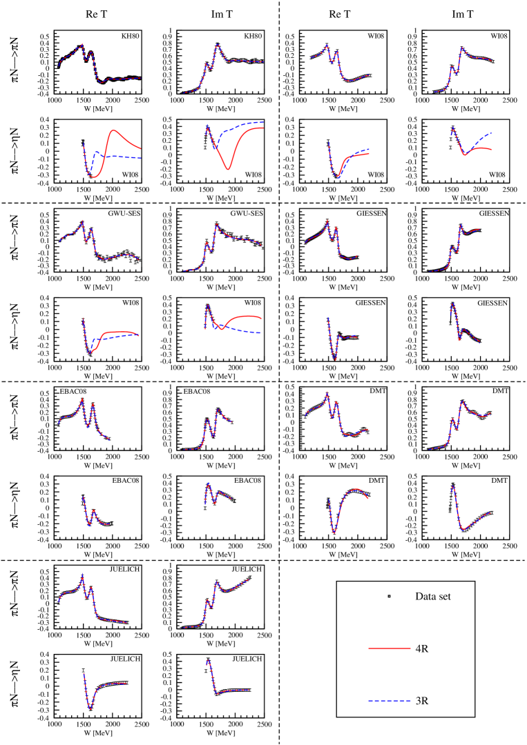
Figure 3: Agreement of 3R and 4R CMB curves with “world input” for two-channel fit.

All obtained pole positions are shown in Fig. 4.

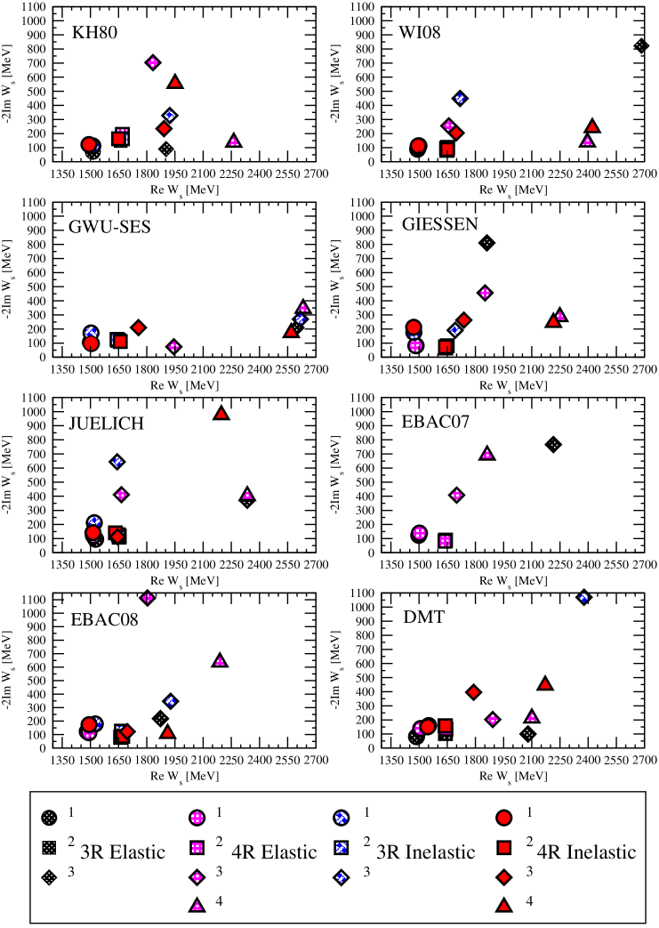
Figure 4: Poles of a “world collection” of PWA.

III.3 Individual comparison

Preliminary considerations

As it has been generally accepted, T-matrix pole positions are the most recommendable singularities to be compared with QCD. However, obtaining them definitely means going into the complex energy plane while having at ones disposal only the physical T-matrix values (values for the real energy). This analytic continuation, however, has to be a model dependent procedure by definition, because there is no a priori rule how to choose the analytic functional form which is to represent a measurable subset out of all possible T-matrix values. Therefore, the reader has to be fully aware that the pole positions we find, and the pole positions given by the original publications have to be different by definition, and the reason is that each investigated “world collection” solution has its own way how to analytically continue the measurable physical T-matrix values. However, comparing the number of needed poles, their distribution and genesis (genuine or dynamic) obtained by our approach with those from original publication is certainly justified. It is also a convenient way to establish whether a certain pole is only a result of a poor knowledge of measured process, or indeed is a genuine singularity needed by the data, but still not yet well established. So, hereafter, we analyze qualitative features of the partial wave singularity structure, and intentionally avoid to compare their numeric values.

III.3.1 KH80

The KH80 amplitudes are essentially single-channel partial wave data with some information about inelastic channels introduced through forward dispersion relations, and analyticity strictly imposed on the level of fitting procedure using Pietarinen expansion Pietarinen . As no assumption on the analytic functional form about partial-wave amplitudes has been done, search for resonance parameters is a separately defined procedure. Breit-Wigner parameters are obtained as a local fit in the resonance region with background contribution unitary added on the level of S matrices, and poles are extracted using single-channel pole position extraction methods (speed plot and Argand diagram). Original publication reported two poles.

In our approach we concur the existence of first two poles, and we find them strongly dominated by the elastic channel.

The third N(2090) pole is in our fit definitely needed. The fourth pole is allowed by our fit in both, single and coupled-channel constellation (improvement of the reduced $\chi_{R}^{2}$), but its quantitative constraint will need more inelastic channels than only $\eta$N. In each configuration numerical values of third and fourth pole are not yet sufficiently well constrained.

III.3.2 GWU-SES and WI08

While the original publication gets the pole positions by analytically continuing energy dependent solution into the complex energy plane, an obvious advantage of our approach is that we can obtain the pole positions independently from both, single energy (GWU-SES) and energy dependent (WI08) VPI/GWU solutions. We have to remember that VPI/GWU pole positions are extracted from the analytic form determined by their Chew-Mandelstam K-matrix approach, which is fitted directly to the data, and not to their single channel solutions. Consequently, the pole positions ”corresponding” to their single energy solutions are by them not yet discussed. In this paper we may use the same formalism for both, single energy and energy dependent solutions, and treat them as an independent input. Hence, we get two sets of solutions.

The general conclusion for both VPI/GWU solutions is the same, and it is very similar to the findings for the KH80 input: we confirm the existence of first two poles, and find them strongly dominated by the elastic channel. The third N(2090) pole is in our fit definitely needed. The fourth pole is allowed by our fit in both, single and two channels constellation (improvement of the reduced $\chi_{R}^{2}$), but its quantitative constraint will need more inelastic channels that $\eta$N.

It is very interesting to compare WI08 with GWU-SES. In spite of the fact that the WI08 solution is seemingly very smooth above the second peak, definitely much smoother than the GWU-SES solution, our model still requires the third and fourth pole almost in a same way for both solutions. The need for a third and fourth pole for the smooth WI08 solution came as a surprise for us. Quantitatively, all pole positions are similar for both solutions: quite well defined for the first two poles, dominantly determined with the elastic channel. Inclusion of inelastic $\eta$N channel data modifies first two pole positions only slightly. However third and fourth pole positions remain strongly influenced.

III.3.3 DMT amplitudes

DMT collaboration has originally looked for the pole positions using the speed plot technique. They have established the existence of three poles, N(1535) , N(1650) and a third pole corresponding to N(2090) - see ref. Che07 . However, triggered by their old research of photo-production channels in which they had established the strong probability for the existence of new S-wave resonant state in the vicinity of 1846 MeV Che03 ; Yan03 , they have recently repeated the analysis and confirmed the existence of this new state at 1880 MeV Mainz2010 .

It is interesting to note that our procedure for DMT amplitudes also indicates the existence of 4 poles. As seen in Fig. 2, our 3-resonant fits do miss some structure in elastic partial waves at higher energies requiring the increase in the number of parameters. Repeated fits with 4 resonances rectify this problem and at the same time show a significant improvement in the reduced $\chi^{2}$. So, our fits concur their latest findings that the DMT S₁₁ solution really contains 4 poles Mainz2010 .

III.3.4 EBAC amplitudes

EBAC has produced three sets of partial wave amplitudes: the first, single channel set where only $\pi$N elastic data have been fitted - EBAC07 - Diaz07 , and two additional sets of amplitudes where data from more than one channel was used to constrain the fit; in this particular case $\pi$N and $\eta$N channels. The unpublished set Saghai2010 in a way supersedes the former 2008 analysis Dur08 where unpleasantly large change of $\pi$N elastic partial waves was needed to accommodate for the second channel. We have analyzed both sets of amplitudes wandering whether a significant change in poles between the two is found. However, as no numeric data for the unpublished set is available to us, we have attempted to ”read off” the data directly from the graph, and that has introduced uncontrollable numeric instabilities. Therefore, we have decided to omit the EBAC10 preliminary data from our analysis until the final results are published.

The EBAC group has in all three analyses used two bare poles, situated relatively high in energy (M $\geq$ 1.8 GeV), and reported two dressed poles corresponding roughly to N(1535) and N(1650). Third and fourth pole have not been found. Just as a preview, we can state that our analysis finds all three solutions very similar. For all three sets we confirm the existence of the first two poles, and they are strongly constrained by the $\pi$N elastic channel alone. However, our fits indicate that significant improvement reduced $\chi^{2}$ is achieved if the third and fourth poles are allowed for. These poles are needed by the fit, but still poorly determined by only two inelastic channels.

III.3.5 Jülich amplitudes

Similarly to many, Jülich group fits their model to VPI/GWU data (to energy dependent WI08 set GWUWEB ), and very much like WI08, obtains a very smooth behavior above 1800 MeV. The only difference with respect to WI08 is a different behavior of high energy tail: while the real part of Jülich amplitudes falls with energy and the imaginary part raises, in case of WI08 amplitudes the result is just opposite. Therefore, a difference between the two should not be found in cross section measurements, but only possibly in some polarization ones. They also report two S₁₁ poles.

Consequently, we expect that our results for pole positions of Jülich amplitudes show a very similar behavior to WI08, and that is fulfilled.

The most prominent feature of our analysis of WI08 amplitudes—that in spite of smooth high energy behavior we need more than two poles to fit the input—is confirmed for Jülich amplitudes as well. It is completely clear that we need at least three poles to satisfactorily reproduce the amplitude shape, and their amplitudes are in our analysis consistent with four S₁₁ poles. Very similar as before, the third and fourth poles are rather undetermined with only two channel constraints. We have discussed the possibility of finding extra poles in Jülich amplitudes with M. Döring in Zagreb last fall Duering2009 , and this possibility has not been entirely ruled out even in analytical continuation Jülich method. They have simply not looked for the pole in that energy range. However, even while this pole might be around 1800 MeV, it must be rather far in the complex energy plane.

III.3.6 Giessen amplitudes

Giessen group also fits GWU-SES data in $\pi$N elastic channel, and gets a reasonable agreement with the input. The main difference with respect to “world collection” amplitudes, again lies in the $\eta$N channel data. Nost results for this channel more or less agree within the N(1535) dominance range, but significantly deviate in the higher energy region.

The Giessen model assumes K-matrix Born approximation where the real part of the Green function is neglected, the analyticity is manifestly violated. Consequently, the comparison of poles obtained in our fit with poles of these amplitudes is more questionable, as the main assumption for the correct analytic continuation—that is the analyticity of the model—is not preserved for both models.

III.4 Primary result: Averages

As the main aim of the paper is to use one method in order to eliminate systematic uncertainties in pole extraction, we summarize our primary results.

III.4.1 $\pi$N elastic channel only

All pole positions and their averages are shown in Figs. 5 and 6.

Three resonant case

As the number of accepted S₁₁ resonances in PDG PDG2010 is three, we first stooped our fit at 3 bare poles.

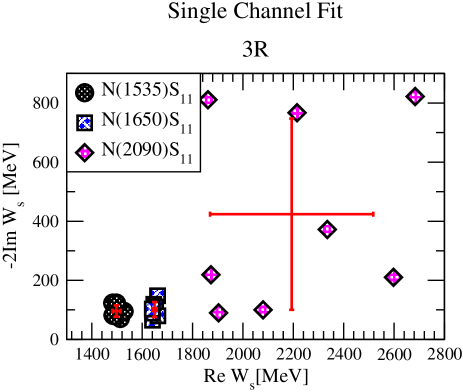
Figure 5: “World collection” of poles for the three resonance single-channel fit.

By inspecting 3R solutions in Table 1 and Fig. 5 we observe:

• First two poles N(1535) and N(1650) are extremely well determined in all PWA.

• We find their average value to be
  
  $\overline{N(1535)\ S_{11}}$   =   $\begin{pmatrix}1498\pm 16\\ 96\pm 20\end{pmatrix}$;
  
  $\overline{N(1650)\ S_{11}}$   =   $\begin{pmatrix}1649\pm 9\\ 101\pm 25\end{pmatrix}$.

• All PWA do need a third pole, but its position is extremely ill-defined; KH80, Giessen and EBAC08 prefer the values between 1700 and 2000 MeV, while the rest have the values above 2000 MeV.

• The resulting average value is poor
  
  $\overline{N(2090)\ S_{11}}$   =   $\begin{pmatrix}2194\pm 324\\ 424\pm 324\end{pmatrix}$.

This separation in two preferred ranges of the third pole among different PWA permits us to speculate whether the fitting rules allow for the existence of the 4-th pole.

Four resonant case

We have repeated the fit with 4-bare poles, and results are collected in Table 1. as 4R solutions. We show the result in Fig. 6.

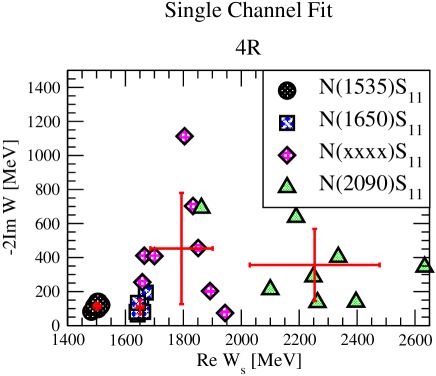
Figure 6: “World collection” of poles for the four resonance single-channel fit.

By inspecting 4R solutions in Table 1 and Fig. 6 we observe:

• We have found that all other PWA if not require, then are at least consistent with the 4 S₁₁ poles, even the EBAC amplitudes which are based on only 2 bare poles input.

• The reduced $\chi^{2}$ is either improved, or at least stays the same for all solutions; that justifies the inclusion of the fourth pole.

• First two poles N(1535) and N(1650) are again very well determined in all PWA

• We find their average value to be
  
  $\overline{N(1535)\ S_{11}}$   =   $\begin{pmatrix}1502\pm 12\\ 114\pm 20\end{pmatrix}$
  
  $\overline{N(1650)\ S_{11}}$   =   $\begin{pmatrix}1651\pm 11\\ 109\pm 42\end{pmatrix}$

• Contrary to our expectations, and in spite of the fact that the reduced $\chi^{2}$ is improved practically everywhere, the scatter in 3rd and 4th pole remain.

• The resulting average value for third and fourth pole is poor
  
  $\overline{N(xxxx)\ S_{11}}$   =   $\begin{pmatrix}1793\pm 108\\ 453\pm 327\end{pmatrix}$
  
  $\overline{N(2090)\ S_{11}}$   =   $\begin{pmatrix}2253\pm 224\\ 356\pm 212\end{pmatrix}$
  
  The existence of the fourth pole is not convincing.

Due to the fact that third and fourth pole poorly couple to the elastic channel that is only used at this instant, we conclude that fitting other channels is inevitable if the improvement on the third and fourth pole parameters is to be achieved.

III.4.2 $\pi$N elastic and $\pi$N $\rightarrow\eta$N data

The poor determination of third and fourth pole for the single channel fit confirms our former findings that inelastic channels are essential for fully constraining all resonant states (scattering matrix poles) - see ref. Ceci06 . The problem with stability of minimization solutions lies in the fact that the $\eta$N channel data are old, scarce, and unreliable (for instance Brown data at higher energies - see discussion in ref. Bat98 ), so $\eta$N channel partial waves are imprecise. Even when being of lower quality, the $\eta$N channel data still represent a valuable constraining condition, because the general trends of $\eta$N channel are to be simultaneously reproduced together with the details of elastic channel, and that is by no means simple. The results of the fit are given in Table 2 and Figs. 7 and 8.

Three resonant case

As the number of accepted S₁₁ resonances in PDG PDG2010 is three, we first stooped our fit at 3 bare poles. We show the result in Fig. 7.

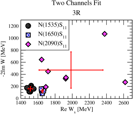
Figure 7: “World collection” of poles for the three resonance, two channels fit.

By inspecting 3R solutions in Table 2 and Fig. 7 we observe:

• First two poles N(1535) and N(1650) are extremely well determined in all PWA.

• We find their average value to be
  
  $\overline{N(1535)\ S_{11}}$   =   $\begin{pmatrix}1512\pm 25\\ 161\pm 36\end{pmatrix}$
  
  $\overline{N(1650)\ S_{11}}$   =   $\begin{pmatrix}1652\pm 12\\ 126\pm 29\end{pmatrix}$.

• If we compare these numbers with the result of single-channel, three resonance fit:
  
  $\overline{N(1535)\ S_{11}}$   =   $\begin{pmatrix}{\it 1498\pm 16}\\ {\it 96\pm 20}\end{pmatrix}$,
  
  $\overline{N(1650)\ S_{11}}$   =   $\begin{pmatrix}{\it 1649\pm 9}\\ {\it 101\pm 25}\end{pmatrix}$,
  
  we see that the difference is within one standard deviation. Real parts of the resonances are almost completely reproduced, while the imaginary parts are slightly shifted downwards.

• All PWA do need a third pole, but it’s position is again extremely ill-defined.

• The resulting average value is poor
  
  $\overline{N(2090)\ S_{11}}$   =   $\begin{pmatrix}1986\pm 373\\ 471\pm 301\end{pmatrix}$.

Four resonant case

We have repeated the fit with 4-bare poles, and results are collected in Table 2. as 4R solutions. We show the result in Fig. 8.

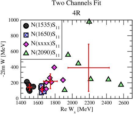
Figure 8: “World collection” of poles for the four resonance, two channels fit.

By inspecting 4R solutions in Table 1 and Fig. 8 we observe:

• We have found that all PWA if not require, then are at least consistent with the 4 S₁₁ poles, even the EBAC amplitudes which are based on only 2 bare poles.

• The reduced $\chi^{2}$ is either improved, or stays the same for all solutions. That justifies the inclusion of the fourth pole.

• First two poles N(1535) and N(1650) are again extremely well determined in all PWA

• We find their average value to be
  
  $\overline{N(1535)\ S_{11}}$   =   $\begin{pmatrix}1502\pm 23\\ 144\pm 39\end{pmatrix}$
  
  $\overline{N(1650)\ S_{11}}$   =   $\begin{pmatrix}1649\pm 13\\ 117\pm 37\end{pmatrix}$.

• The resulting average value for third and fourth pole are:
  
  $\overline{N(xxxx)\ S_{11}}$   =   $\begin{pmatrix}1745\pm 80\\ 220\pm 95\end{pmatrix}$
  
  $\overline{N(2090)\ S_{11}}$   =   $\begin{pmatrix}2191\pm 241\\ 392\pm 301\end{pmatrix}$.

• The scatter in the 3rd pole is significantly reduced, and the indications for its existence are strong.

• The existence of the fourth pole is strongly indicated, but still not quite convincing.

• If we compare these numbers with the result of single-channel, four resonance fit:
  
  $\overline{N(1535)\ S_{11}}$   =   $\begin{pmatrix}{\it 1502\pm 12}\\ {\it 114\pm 20}\end{pmatrix}$,
  
  $\overline{N(1650)\ S_{11}}$   =   $\begin{pmatrix}{\it 1651\pm 11}\\ {\it 109\pm 42}\end{pmatrix}$,
  
  $\overline{N(xxxx)\ S_{11}}$   =   $\begin{pmatrix}{\it 1793\pm 108}\\ {\it 453\pm 325}\end{pmatrix}$,
  
  $\overline{N(2090)\ S_{11}}$   =   $\begin{pmatrix}{\it 2253\pm 224}\\ {\it 356\pm 212}\end{pmatrix}$,

  we conclude:
  the $\eta$N channel data have confirmed the good constraint on N(1535) and N(1650) S₁₁ states, they have improved the confidence limits for the existence of the new N(xxxx) S₁₁ state, but they are definitely insufficient to constrain the fourth S₁₁ pole.
  
  Therefore, other channel partial waves have to be included.

IV Conclusions

We have offered one model, the Zagreb realization of CMB model, for extracting pole positions from a “world collection” of partial-wave amplitudes which we treat as partial wave input data, and extracted the results. Using only one method enables us to make a statistical analysis of partial wave poles in a manner that we avoid the systematic error caused by the different assumptions on the partial wave analytic function form. We have in details explained the idea, and presented the results for the S₁₁ partial wave only.

We have analyzed the single channel fit (only one channel data are used to constrain the fit), and in details investigated what are the consequences of enlarging it to a two-channel one with the $\eta$N channel. We have concluded that even low quality data in the second channel are sufficient to notably constrain the arbitrariness of the poorly determined poles. However, we also concluded that for the third and fourth S-wave poles, $\eta$N channel is not sufficient.

We found that the first two S₁₁ poles are extremely well defined by elastic channel and that the included inelastic $\eta$N channel introduces only small modifications of the elastic channel result.

We have shown that all members of the partial wave “world collection”, in spite of the fact that some of them have assumed only two S-wave resonant states, are consistent with at least three T-matrix poles. We have also demonstrated that there is a strong statistical indications that the fourth pole is present in each of the “world collection” member, despite the fact that no one has seen it up to now. The exception is the latest DMT analyses Mainz2010 where all four poles are detected. The new S₁₁ pole we have found can be identified with the S₁₁(1846) pole seen in photo-production channel by the DMT collaboration Che03 ; Yan03 .

We affirm that the results of the 4-resonant, double channel fit should be treated as a final result, and we offer the world average:

$${\rm N}(1535)\ {\rm S}_{11}=\footnotesize{\begin{pmatrix}1502\pm 23\\ 144\pm 39\end{pmatrix}}$$ (12)

$${\rm N}(1650)\ {\rm S}_{11}=\footnotesize{\begin{pmatrix}1649\pm 13\\ 117\pm 37\end{pmatrix}}$$

$${\rm N}(xxxx)\ {\rm S}_{11}=\footnotesize{\begin{pmatrix}1745\pm 80\\ 220\pm 95\end{pmatrix}}$$

$${\rm N}(2090)\ {\rm S}_{11}=\footnotesize{\begin{pmatrix}2191\pm 241\\ 392\pm 301\end{pmatrix}}$$

References

- (1) R.H. Dalitz and R.G. Moorhouse, Proc. Roy. Soc. Lond. A318 (1970) 279-298.
- (2) S. Mandelstam, Phys. Rev. 112 (1958) 1344.
- (3) A.D. Martin, T.D. Spearman, Elementary particle theory, North-Holland Publishing Company, Amsterdam, 1970.
- (4) R. A. Arndt et all., Phys. Rev. C 74 (2006) 045205.
- (5) D. M. Manley and E. M. Salesky, Phys. Rev D 45 (1992) 4002.
- (6) M. Manley, Phys. Rev. D 51 (1995) 4837.
- (7) R. E. Cutkosky et all., Phys. Rev. D 20 (1979) 2804.
- (8) M. Batinić, et al., Phys. Rev. C 51, 2310 (1995); M. Batinić, et al., Physica Scripta 58, 15, (1998).
- (9) T. P. Vrana, S. A. Dytman, T. -S. H. Lee, Phys. Rep. 328 (2000) 181.
- (10) S.M. Flatté, Phys. Lett. B 63, 224 (1976); S. M. Flatté et al., Phys. Lett. B 38, 232 (1972).
- (11) N. G. Kelkar, M. Nowakowski, K. P. Khemchandani, Sudhir R. Jain, Nucl.Phys. A 730 (2004) 121-140.
- (12) G. Höhler, in Pion-Nucleon Scattering, Landolt-Börnstein, Vol I/9b2 (Springer-Verlag, Berlin, 1983); G. Höhler, A. Schulte, Newsletter, 7 (1992) 407.
- (13) G. Höhler, Against Breit-Wigner parameters – a pole-emic, in C. Caso et al. [Particle Data Group], Eur. Phys. J. C 3, 624 (1998).
- (14) G. Höhler, RESULTS ON (1232) RESONANCE PARAMETERS: A NEW N PARTIAL WAVE ANALYSIS, in NSTAR2001, Proceedings of the Workshop on the Physics of Excited Nucleons, Edts. D. Drechsel, L. Tiator, World Scientific Publishing Co. (2001), Pg.185.
- (15) K. Nakamura et al. (Particle Data Group), J. Phys. G 37, 075021 (2010).
- (16) S, Ceci, J. Stahov, A. Švarc, S. Watson and B. Zauner, Phys. Rev. D 77, 116007 (2008).
- (17) L. Tiator, S.S. Kamalov, S. Ceci, G. Y. Chen, D. Drechsel, A. Švarc and S. N. Yang, Phys. Rev. C 82, 055203 (2010).
- (18) L. Eisenbud, disertation, Princeton, June 1948 (unpublished)
- (19) E. P. Wigner, Phys. Rev. 98, 145 (1955)
- (20) E. P. Wigner, L. Eisenbud Phys. Rev. 72, 29 (1947)
- (21) D. Bohm, Quantum Theory (Prentice-Hall, New York, 1951)
- (22) N. Suszuki, T. Sato, T. -S. H. Lee, Proceedings of the Menu2007 11th International Conference on Meson-nucleon Physics and the structure of the Nucleon, Jüelich 2007, edited by H. Machner, S Krewald, eConf C070910 (2007) 407
- (23) G. F. Chew and S. Mandelstam, Phys. Rev. 119, 467 (1960).
- (24) J. A. Oller and E. Oset,Phys. Rev. D 60, 074023 (1999).
- (25) V.V. Anisovich, International Journal of Modern Physics, A 21, 3615 (2006).
- (26) R. A. Arndt, W.J. Briscoe, I.I. Strakovsky, R.L. Workman, and M.M. Pavan, Phys. Rev. C69, 035213 (2004).
- (27) N. Suzuki, T. Sato and T. -S. H, Lee, Phys. Rev. C 79, 025205 (2009).
- (28) T. Feuster and U. Mosel1, Phys. Rev. C 58, 457 (1998).
- (29) Guan-Yeu Chen, Sabit Kamalov, Shin Nan Yang, Dieter Drechsel, Lothar Tiator, Nuclear Physics A 723, 447 (2003).
- (30) Guan Yeu Chen, S. S. Kamalov, Shin Nan Yang, D. Drechsel and L. Tiator, Phys. Rev. C76, 035206 (2007).
- (31) V. Shklyar, H. Lenske, U. Mosel, Phys. Rev. C 72, 015210 (2005), and private communication.
- (32) S. N. Yang, G.-Y. Chen, S. S. Kamalov, D. Drechsel and L. Tiator, Nucl. Phys. A 721 401c (2003); S. N. Yang, G.-Y. Chen, S. S. Kamalov, D. Drechsel and L. Tiator, Int. Journal of Modern Physics, A 20 1656 (2005).
- (33) H. Osmanović, S. Ceci, A. Švarc, M. Hadžimehmedović and J. Stahov, submitted to Phys. Rev. C.
- (34) M. Batinić, et al., Phys. Rev. C 51, 2310 (1995); M. Batinić, et al., Physica Scripta 58, 15, (1998).
- (35) R. E. Cutkosky et al., Phys. Rev. D 20, 2839 (1979).
- (36) http://gwdac.phys.gwu.edu/analysis/pin_analysis.html.
- (37) B. Juliá-Díaz, T.-S. H. Lee,1 A. Matsuyama, and T. Sato, Phys. Rev. C 76, 065201 (2007).
- (38) J. Durand, B. Juliá-Díaz, T.-S. H. Lee, B. Saghai, and T. Sato, Rev. C 78, 025204 (2008).
- (39) M. Döring, C. Hanhart,, F. Huang, S. Krewald, U.-G. Meissner, Nucl.Phys, A 829, 170 (2009); C. Schütz, J. Haidenbauer, J. Speth and J. W. Durso, Phys. Rev. C 57 1464 (1998); O. Krehl, C. Hanhart, S. Krewald and J. Speth, Phys. Rev. C 62 025207 (2000); A. M. Gasparyan, J. Haidenbauer, C. Hanhart and J. Speth, Phys. Rev. C 68 045207 (2003).
- (40) S. Ceci, A. Švarc, and B. Zauner, Phys. Rev. Lett. 97, 062002 (2006).
- (41) M. Döring, B. Diaz private communications.
- (42) E. Pietarinen, Nuovo Cimento, 12A, 522 (1972).
-
(43)
B. Saghai, et al, EBAC meeting on ”Extraction of nucleon resonances”, May 24 - 26, 2010, JLab, Virginia, USA;
http://ebac-theory.jlab.org/workshop_meeting/m2010/talks/Saghai-ebac-m2010.pdf