Variational approach to complicated similarity solutions of higher-order nonlinear PDEs. II

Abstract.

This paper continues the study began in [11, 12] of the Cauchy problem for $(x,t)\in{\mathbb{R}}^{N}\times{\mathbb{R}}_{+}$ for three higher-order degenerate quasilinear partial differential equations (PDEs), as basic models,

$$\begin{matrix}u_{t}=(-1)^{m+1}\Delta^{m}(|u|^{n}u)+|u|^{n}u,\qquad\,\quad\vskip 3.0pt plus 1.0pt minus 1.0pt\\ u_{tt}=(-1)^{m+1}\Delta^{m}(|u|^{n}u)+|u|^{n}u,\qquad\quad\vskip 3.0pt plus 1.0pt minus 1.0pt\\ u_{t}=(-1)^{m+1}[\Delta^{m}(|u|^{n}u)]_{x_{1}}+(|u|^{n}u)_{x_{1}},\end{matrix}$$

where $n>0$ is a fixed exponent and $\Delta^{m}$ is the $(m\geq 2)$th iteration of the Laplacian. A diverse class of degenerate PDEs from various areas of applications of three types: parabolic, hyperbolic, and nonlinear dispersion, is dealt with. General local, global, and blow-up features of such PDEs are studied on the basis of their blow-up similarity or travelling wave (for the last one) solutions.

In [11, 12], Lusternik–Schnirel’man category theory of variational calculus and fibering methods were applied. The case $m=2$ and $n>0$ was studied in greater detail analytically and numerically. Here, more attention is paid to a combination of a Cartesian approximation and fibering to get new compactly supported similarity patterns. Using numerics, such compactly supported solutions constructed for $m=3$ and for higher orders. The “smother” case of negative $n<0$ is included, with a typical “fast diffusion-absorption” parabolic PDE:

$$u_{t}=(-1)^{m+1}\Delta^{m}(|u|^{n}u)-|u|^{n}u,\quad\mbox{where}\quad n\in(-1,0),$$

which admits finite-time extinction rather than blow-up. Finally, a homotopy approach is developed for some kind of classification of various patterns obtained by variational and other methods. Using a variety of analytic, variational, qualitative, and numerical methods allows to justify that the above PDEs admit an infinite countable set of countable families of compactly supported blow-up (extinction) or travelling wave solutions.

1. Introduction: higher-order blow-up and compacton models

A general physical and PDE motivation of the present research can be found in [11, 12], together with basic history and related key references, so we just briefly comment on where quasilinear elliptic problems under consideration are coming from.

1.1. (I) Combustion-type models with blow-up

Our first model is a quasilinear degenerate $2m$th-order parabolic equation of the reaction-diffusion (combustion) type:

(1.1) $$u_{t}=(-1)^{m+1}\Delta^{m}(|u|^{n}u)+|u|^{n}u\quad\mbox{in}\quad{\mathbb{R}}^{N}\times{\mathbb{R}}_{+},$$

where $n>0$ is a fixed exponent, $m\geq 2$ is integer, and $\Delta$ denotes the Laplace operator in ${\mathbb{R}}^{N}$. Physical, mathematical, and blow-up history of (1.1) for the standard classic case $m=1$ and $m\geq 2$ is explained in [11, 12, § 1]. Consider regional blow-up solutions of (1.1)

(1.2) $$u_{\rm S}(x,t)=(T-t)^{-\frac{1}{n}}f(x)\quad\mbox{in}\quad{\mathbb{R}}^{N}\times(0,T)$$

in separable variables, where $T>0$ is the blow-up time. Then the similarity blow-up profile $f=f(x)$ solves a quasilinear elliptic equation of the form

(1.3) $$(-1)^{m+1}\Delta^{m}(|f|^{n}f)+|f|^{n}f=\frac{1}{n}\,f\quad\mbox{in}\quad{\mathbb{R}}^{N}.$$

This reduces to the following semilinear equation with a non-Lipschitz nonlinearity:

$$F=|f|^{n}f\quad\Longrightarrow\quad\mbox{$(-1)^{m+1}\Delta^{m}F+F-\frac{1}{n}\,\big{|}F\big{|}^{-\frac{n}{n+1}}F=0\quad\mbox{in}\,\,\,{\mathbb{R}}^{N}.$}$$

Scaling out the multiplier $\frac{1}{n}$ in the nonlinear term yields

(1.4) $$F\mapsto n^{-\frac{n+1}{n}}F\quad\Longrightarrow\quad\framebox{$(-1)^{m+1}\Delta^{m}F+F-\big{|}F\big{|}^{-\frac{n}{n+1}}F=0\quad\mbox{in}\,\,\,{\mathbb{R}}^{N}.$}$$

For $N=1$, this is a simpler ordinary differential equation (an ODE):

(1.5) $$F\mapsto n^{-\frac{n+1}{n}}F\quad\Longrightarrow\quad\framebox{$(-1)^{m+1}F^{(2m)}+F-\big{|}F\big{|}^{-\frac{n}{n+1}}F=0\quad\mbox{in}\,\,\,{\mathbb{R}}.$}$$

According to (1.2), the elliptic problems (1.4) and the ODE (1.5) for $N=1$ are responsible for the possible “geometrical shapes” of regional blow-up described by the higher-order combustion model (1.1).

Remark: relation to ODEs from extended KPP theory. There exists vast mathematical literature, starting essentially from the 1980s, devoted to the fourth-order ODEs (looking rather analogously to that in (1.5) for $m=2$)

(1.6) $$F^{(4)}=\beta F^{\prime\prime}+F-F^{3}\quad\mbox{in}\quad{\mathbb{R}},$$

where $\beta>0$ is a parameter. This ODE also admits a complicated set of solutions with various classes of patterns and even with chaotic features. We refer to Peletier–Troy’s book [26] for the most diverse account, as well as to papers [18, 34], where a detailed and advanced solution description for (1.6) is obtained by combination of variational and homotopy theory. Regardless their rather similar forms, the ODEs (1.5) belong to a completely different class of equations with non-coercive operators, unlike in (1.6). Therefore, direct homotopy approaches and several others, that used to be rather effective for (1.6), fail in principle for (1.5). In this sense, (1.5) is similar to the cubic ODE to be studied in Section 6:

(1.7) $$\framebox{$F^{(4)}=-F+F^{3}\quad\mbox{in}\quad{\mathbb{R}},$}$$

of course, excluding complicated oscillatory behaviour at finite interfaces, which are obviously nonexistent for analytic nonlinearities. However, we claim that the sets of solutions of (1.5), with $m=2$, and of (1.7) are equivalent, though, not having a rigorous proof, we will devote some efforts to a homotopy approach connecting solutions of such smooth (analytic) and non-smooth ODEs. Thus, though going to develop homotopy approaches for classifying solutions of (1.5) (Section 4), our main tool to describe countable families of solutions $\{F_{l}\}$ is a combination of Lusternik–Schnirel’man category-genus theory [21] and the fibering method [27, 28].

Thus, we show that ODEs (1.5), as well as the PDE (1.4), admit infinitely many countable families of compactly supported solutions, and the whole solution set exhibits certain chaotic properties. Our analysis will be based on a combination of analytic (variational and others), numerical, and some more formal techniques. Explaining existence, multiplicity, and asymptotics for the nonlinear problems involved, we state and leave several open difficult mathematical problems. Meantime, let us characterize other models involved.

1.2. (II) Regional blow-up in quasilinear hyperbolic equations

Consider next the $2m$th-order hyperbolic counterpart of (1.1),

(1.8) $$u_{tt}=(-1)^{m+1}\Delta^{m}(|u|^{n}u)+|u|^{n}u\quad\mbox{in}\quad{\mathbb{R}}^{N}\times{\mathbb{R}}_{+}.$$

The blow-up solutions take a similar form with a different exponent $-\frac{2}{n}$ instead of $-\frac{1}{n}$:

(1.9) $$u_{\rm S}(x,t)=(T-t)^{-\frac{2}{n}}f(x),$$

where $F=|f|^{n}f$, after scaling, solves the same elliptic equation (1.4).

1.3. (III) Nonlinear dispersion equations and compactons

Such rather unusual PDEs in $N$-dimensions (the origin is integrable PDEs and other areas) take the form

(1.10) $$u_{t}=(-1)^{m+1}[\Delta^{m}(|u|^{n}u)]_{x_{1}}+(|u|^{n}u)_{x_{1}}\quad\mbox{in}\quad{\mathbb{R}}^{N}\times{\mathbb{R}}_{+},$$

where the right-hand side is the derivative $D_{x_{1}}$ of that in the parabolic counterpart (1.1). Then the elliptic problem (1.4) occurs when studying travelling wave (TW) solutions of (1.10). Note that, as being PDEs with nonlinear dispersion mechanism, (1.10) and other NDEs listed below admit shock waves and other discontinuous solutions. Here, we study smooth solutions and do not touch difficult entropy-like approaches for such shock and rarefaction waves and refer to [15, § 4.2] and [14] for an account to such phenomena.

Thus, for the PDE (1.10), looking for a TW compacton (i.e., a solution having all the time compact support; see key references in [11, § 1]) moving in the $x_{1}$-direction only,

(1.11) $$u_{\rm c}(x,t)=f(y_{1},x_{2},...,x_{N}),\,\,\,y_{1}=x_{1}-\lambda t,\quad\mbox{where}\quad\lambda=-\frac{1}{n},$$

we obtain on integration in $y_{1}$ the elliptic problem (1.4). Analogously, for the higher-order evolution extension of nonlinear dispersion PDEs,

$$D_{t}^{k}u=D^{k}_{x_{1}}\bigl{[}(-1)^{m+1}\Delta^{m}(|u|^{n}u)+|u|^{n}u\bigr{]}\quad\mbox{in}\quad{\mathbb{R}}^{N}\times{\mathbb{R}}_{+}\quad(k\geq 2),$$

to get the same PDE (1.4), the compacton (1.11) demands the following wave speed:

$$(-\lambda)^{k}=\frac{1}{n}.$$

1.4. (IV) PDEs with “fast diffusion” operators: parabolic, Schrödinger, hyperbolic, and nonlinear dispersion models

This is about negative exponents:

(1.12) $$n\in(-1,0),$$

which generate other types of elliptic equations of interest. To connect such problems with typical models of diffusion-absorption type, consider the following parabolic PDE:

(1.13) $$u_{t}=(-1)^{m+1}\Delta^{m}(|u|^{n}u)-|u|^{n}u\quad\mbox{in}\quad{\mathbb{R}}^{N}\times{\mathbb{R}}_{+}\quad(-1<n<0),$$

with the strong non-Lipschitz at $u=0$ absorption term. It is well known that such PDEs describe finite-time extinction phenomenon instead of blow-up. See [16, Ch. 4,5] for $m=1$ and [8, 32] for $m\geq 2$ for necessary references and history of strong absorption phenomena. Therefore, the similarity solution takes an analogous to (1.2) form with the positive exponent $-\frac{1}{n}>0$, so that $u(x,T^{-})\equiv 0$, while $f$ solves a similar elliptic equation (cf. (1.3))

(1.14) $$(-1)^{m+1}\Delta^{m}(|f|^{n}f)-|f|^{n}f=\frac{1}{n}\,f\quad\mbox{in}\,\,\,{\mathbb{R}}^{N}.$$

By the scaling as in (1.4) (recall that $n<0$), we eventually obtain the semilinear elliptic problem with a sufficiently smooth nonlinearity:

(1.15) $$\framebox{$(-1)^{m+1}\Delta^{m}F-F+\big{|}F\big{|}^{\alpha}F=0\quad\mbox{in}\,\,\,{\mathbb{R}}^{N},\quad\mbox{where}\quad\alpha=-\frac{n}{n+1}>0.$}$$

The nonlinearity is now $C^{1}$ at $F=0$, so the solutions are classic. For instance, for $m=2$ and $n=-\frac{2}{3}$, we obtain equation with a cubic analytic nonlinearity:

(1.16) $$\Delta^{2}F=-F+F^{3}\quad\mbox{in}\quad{\mathbb{R}}^{N}.$$

For $N=1$, this is the ODE (1.7). Indeed, these equations do not admit solutions with finite interfaces and exhibit exponentially decaying oscillatory behaviour at infinity. We show that the total set of such “effectively” spatially localized patterns well matches those ones for $n>0$ always having finite interfaces.

As a connection to another classic PDE area and applications, let us note that, for $m=1$, we obtain the classic second-order case of the ground state equation [6]

(1.17) $$\Delta F-F+F^{3}=0\quad\mbox{in}\quad{\mathbb{R}}^{N}.$$

This elliptic problem is key in blow-up analysis of the critical nonlinear Schrödinger equation (NLSE)

$${\rm i}\,u_{t}=-\Delta u-|u|^{p-1}u,\quad p=p_{0}=1+\frac{4}{N},\,\,N=2,\quad\mbox{and}\quad u(x,t)={\mathrm{e}}^{{\rm i}\,t}F(x);$$

see Merle–Raphael [22]–[24] as a guide. The solution $F$ of (1.17) is strictly positive (with exponential decay at infinity) and is unique up to translations, while the ground state $F_{0}$ for (1.16) is oscillatory at infinity, to say nothing about a huge variety of other, Lusternik–Schnirel’man or not, solutions. Thus, (1.16) is the ground state equation for the fourth-order NLSE

$${\rm i}\,u_{t}=\Delta^{2}u-|u|^{p-1}u\quad\mbox{in}\quad{\mathbb{R}}^{N}\times{\mathbb{R}}_{+},\quad\mbox{where}\quad p=p_{0}=1+\frac{8}{N}\,\,\,(N=4).$$

Analogous similarity analysis is performed for the corresponding “fast diffusion” hyperbolic equation (the extinction patterns are given by (1.9))

(1.18) $$u_{tt}=(-1)^{m+1}\Delta^{m}(|u|^{n}u)-|u|^{n}u\quad\mbox{in}\quad{\mathbb{R}}^{N}\times{\mathbb{R}}_{+}\quad(-1<n<0),$$

and for the nonlinear “fast dispersion” PDE

(1.19) $$u_{t}=(-1)^{m+1}[\Delta^{m}(|u|^{n}u)]_{x_{1}}-(|u|^{n}u)_{x_{1}}\quad\mbox{in}\quad{\mathbb{R}}^{N}\times{\mathbb{R}}_{+}\quad(-1<n<0),$$

where the moving TW profiles are as in (1.11).

1.5. Main goals and connections with previous results

It turns out that such profiles $F$ solving (1.4) have rather complicated local and global structure. The study of equations (1.4) and (1.5) was began in [11], where the following goals were posed:

(i) Problem “Blow-up”: proving finite-time blow-up in the parabolic (and hyperbolic) PDEs under consideration [11, § 2];

(ii) Problem “Existence and Multiplicity”: existence and multiplicity for elliptic PDEs (1.4) and the ODEs (1.5) for $m\geq 2$ [11, § 3];

(iii) Problem “Oscillations”: the generic structure of oscillatory solutions of (1.5) near interfaces for arbitrary $m\geq 2$ [11, § 4]; and

(iv) Problem “Numerics”: numerical study of all families of $F(x)$ for $m=2$ [11, § 5].

The non-Lipschitz problem (1.1) possesses so complicated set of admissible compactly supported solutions (note that Lusternik–Schnirel’man category theory detects only a single countable subset), that using effective MatLab (or other similar or advanced) numerical techniques for classifying the critical points becomes an unavoidable tool of any analytic-numerical approach, which cannot be dispensed with at all. We recall that in [11, § 3] the identification of Lusternik–Schnirel’man sequence of critical values was confirmed numerically only (and for $m=2$ essentially).

Therefore, in the present paper, in Section 3, we begin by continuing achieving the goal (iv) for the sixth-order case $m=3$:

(iv^′) Problem “Numerics”: numerical study of all families of $F(x)$ for $m\geq 3$ (Section 3).

In addition, we also aim new targets:

(ii^′) Problem “Existence and Multiplicity”: using variational Lusternik–Schnirel’man approach and fibering with an auxiliary Cartesian approximation of critical points (Section 2);

(v) Problem “Fast diffusion”: $n\in(-1,0)$, where smoother elliptic problems (1.15) occur (extinction in Sections 5 and existence-multiplicity in Section 6).

Finally, for both the non-smooth (1.4) and smooth (1.15) problems, we pose:

(vi) Problem “Sturm Index”: classification of various patterns according to their spatial shape for both (1.4) and (1.15) (Sections 4, 6, and 7). [For $m=1$, this is governed by classic Sturm’s First Theorem on zero sets.]

Thus, we are introducing three classes, (I), (II), (III), of nonlinear higher-order PDEs in ${\mathbb{R}}^{N}\times{\mathbb{R}}_{+}$ including similar fast diffusion ones (IV). These are representatives of PDEs of three different types. However, it will be shown that these exhibit quite analogous evolution features (if necessary, up to replacing blow-up by moving travelling waves or extinction behaviour), and coinciding complicated countable sets of evolution patterns. This reveals an exiting feature of a certain unified principle of singularity formation phenomena in general nonlinear PDE theory, which we would like to believe in, but which is very difficult to justify more rigorously.

1.6. On extensions to essentially quasilinear equations

The three-fold unity of PDE classes (I)–(III) is available for other types of nonlinearities. In Section 8, we briefly discuss the following classes of equations with fourth-order $p$-Laplacian operators (here $n=p-2>0$):

(1.20) $$\begin{matrix}{\bf(I)}\quad u_{t}=-\Delta(|\Delta u|^{n}\Delta u)+|u|^{n}u\quad(\mbox{parabolic}),\,\,\vskip 3.0pt plus 1.0pt minus 1.0pt\vskip 3.0pt plus 1.0pt minus 1.0pt\\ {\bf(II)}\quad u_{tt}=-\Delta(|\Delta u|^{n}\Delta u)+|u|^{n}u\quad(\mbox{hyperbolic}),\vskip 3.0pt plus 1.0pt minus 1.0pt\vskip 3.0pt plus 1.0pt minus 1.0pt\\ {\bf(III)}\quad u_{t}=-\big{[}\Delta(|\Delta u|^{n}\Delta u)\big{]}_{x_{1}}+(|u|^{n}u)_{x_{1}}\quad(\mbox{NDE}).\end{matrix}$$

It turns out that these equations admit similar blow-up or compacton (for the NDE (III)) solutions that are governed by variational elliptic problems with similar countable variety of oscillatory compactly supported solutions. As a first step, an approach to blow-up of solutions of the parabolic equation (1.20) for $N=1$ and some other related results on similarity solutions can be found in [9].

Thus, these cases are more difficult and are essentially quasilinear, since the resulting elliptic problems cannot be reduced to semilinear equations such as (1.5).

1.7. Towards non-variational problems: branching

Principally more difficult problems occur under a slight change of the lower-order nonlinearity in (1.20):

(1.21) $$|u|^{n}u\mapsto|u|^{p}u,\quad\mbox{with}\quad p>n.$$

This leads to non-variational elliptic problems, to be also briefly discussed in Section 8 using the idea of branching of proper solutions at $p=n$ from the similarity profiles studied above. Proving existence of countable sets of solutions for such non-potential operators reveals a number of open problems of a higher level of complexity.

2. Other families of patterns: Cartesian approximation and fibering

Application of the Lusternik–Schnirel’man category theory to constructing a countable family of solutions of (1.5) is explained in [11, § 3]. This allowed us to detect the so-called basic family of patterns $\{F_{l}\}$, which has been shown for $N=1$ in a number of figures in [11, § 4]. For convenience, we restate the Lusternik–Schnirel’man/fibering result in [11, § 3.2]:

Proposition 2.1.

The elliptic problem $(\ref{S2NN})$ has at least a countable set of different solutions denoted by $\{F_{l},\,l\geq 0\}$, each one $F_{l}$ obtained as a critical point of the functional

(2.1) $${E}(F)=-{\displaystyle\frac{1}{2}\int_{B_{R}}|\tilde{D}^{m}F|^{2}+\frac{1}{2}\int_{B_{R}}F^{2}-\frac{1}{\beta}\,\int_{B_{R}}|F|^{\beta},\quad\beta=\frac{n+2}{n+1}\in(1,2)},\,\,\,n>0,$$

in $W^{2,m}_{0}(B_{R})$ in a ball $B_{R}$ with a sufficiently large radius $R=R(l)>0$.

2.1. Basic computations

We next develop approaches for obtaining other patterns, which are not detected in Proposition 2.1 by Lusternik–Schnirel’man and classical fibering techniques.

In order to construct other families of solutions (see Section 3 for illustrations of those for $m=3$), we need an auxiliary approximation of patterns. Namely, we first perform the Cartesian decomposition

(2.2) $$F=h+w,$$

where $h\in W^{2,m}_{0}(B_{R})$ is a smooth “step-like function” that takes the equilibrium values $\pm 1$ and 0 on some disjoint subsets of $B_{R}$ (with a smooth connections in between). Sufficiently close to the boundary points, we always have $h(y)=0$. For instance, in one dimension for getting the patterns in Figure 1, we take $h(y)$ as a smooth approximation of the step function, which takes values $\pm 1$ and 0 on the intervals of oscillations of the solution about these equilibria.

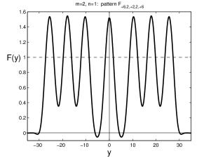
(a) $\sigma=\{+6,2,+2,2,+6\}$

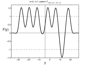
(b) $\sigma=\{+6,2,+4,1,-2,1+2\}$

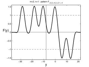
(c) $\sigma=\{+2,2,+4,2,+2,1,-4\}$

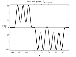
(d) $\sigma=\{+6,3,-4,2,-6\}$

Figure 1. Various patterns for $m=2$ and $n=1$.

In other words, we are going to perform the radial fibering not about the origin but about the non-trivial point $h$, which plays the role of an initial approximation of the pattern that we are interested in. Obviously, the choice of such $h$’s is of principal importance, which thus should be done very carefully.

Substituting (2.2) into the functional yields the new one,

(2.3) $$\begin{matrix}\hat{E}(w)=E(h+w)=-\displaystyle\frac{1}{2}\int_{B_{R}}|\tilde{D}^{m}h|^{2}+\frac{1}{2}\displaystyle\int_{B_{R}}h^{2}+L_{0}(h)w\qquad\quad\vskip 3.0pt plus 1.0pt minus 1.0pt\vskip 3.0pt plus 1.0pt minus 1.0pt\\ -H_{0}(w)-\displaystyle{\frac{1}{\beta}\,\int_{B_{R}}|h+w|^{\beta}},\qquad\quad\end{matrix}$$

where by $L_{0}$ we denote the linear functional

$$L_{0}(h)w=-\displaystyle\int_{B_{R}}\tilde{D}^{m}h\cdot\tilde{D}^{m}w+\displaystyle\int_{B_{R}}hw.$$

We next apply the fibering approach by setting, as usual,

(2.4) $$w=r(v)v,\quad v\in{\mathcal{H}}_{0},\quad\mbox{whence}$$

(2.5) $$\begin{matrix}\hat{H}(r,v)=E(h+r(v)v)=-\displaystyle\frac{1}{2}\int_{B_{R}}|\tilde{D}^{m}h|^{2}+\frac{1}{2}\displaystyle\int_{B_{R}}h^{2}+r\,L_{0}v\qquad\quad\vskip 3.0pt plus 1.0pt minus 1.0pt\vskip 3.0pt plus 1.0pt minus 1.0pt\\ +\,\displaystyle{\frac{1}{2}\,r^{2}-\frac{1}{\beta}\,}\displaystyle\int_{B_{R}}|h+rv|^{\beta}.\qquad\quad\end{matrix}$$

In order to find the absolute minimum point, we need to solve the scalar equation $\hat{H}^{\prime}_{r}=0$,

(2.6) $$\hat{H}_{r}(r,v)\equiv r-\displaystyle\int_{B_{R}}|h+rv|^{\beta-2}(h+rv)v+L_{0}(h)v=0.$$

For $h=0$, this coincides with the standard equation derived in [11, § 3], and has three roots, $r_{0}(v)=0$ and

(2.7) $$r_{\pm}=r_{\pm}(v),$$

which are positive and negative respectively. For $h\not=0$, these roots exist and are slightly deformed for sufficiently small $h$. For large $h$, one of the roots $r_{\pm}(v)$ may disappear, and at this instance the resulting functional (q.v. below) may loose its smoothness. To distinguish the roots, we observe that

(2.8) $$\begin{matrix}r_{-}(v)<0\,\,\,\mbox{always exists and smooth if\, $J(h,v)\equiv-\displaystyle\int_{B_{R}}|h|^{\beta-2}hv+L_{0}(h)v>0$},\quad\vskip 3.0pt plus 1.0pt minus 1.0pt\vskip 3.0pt plus 1.0pt minus 1.0pt\\ r_{+}(v)>0\,\,\,\mbox{always exists and smooth if \, $J(h,v)\equiv-\displaystyle\int_{B_{R}}|h|^{\beta-2}hv+L_{0}(h)v<0$}.\quad\end{matrix}$$

Thus, calculating the extremum point $r_{\pm}(v)$ (when exists) from (2.6) and substituting into (2.5) yields the new functional

(2.9) $$\tilde{H}(v)=\hat{H}(r_{\pm}(v),v)\quad\mbox{on}\quad{\mathcal{H}}_{0},\quad\mbox{being even, since}\quad r_{\pm}(-v)=-r_{\pm}(v).$$

Therefore, if (2.9) is smooth on an appropriate branch $r_{\pm}$, this gives a set of critical point $\{v_{k}\}$, as above. Moreover, in a neighbourhood of any critical points $v_{k}$ satisfying (2.8), i.e., $J(h,v_{k})>0$ or $<0$, the corresponding branches $r_{\pm}(v)$ are smooth for $v\approx v_{k}$ (and hence along a minimizing sequence $\{v_{k}^{j}\}\to v_{k}$), so that (2.9) is sufficiently regular. Even in the delicate case, when $J(h,v_{k})=0$ and $r=0$ is an inflection point of $\hat{H}_{r}(r,v_{k})$, i.e.,

$$\hat{H}_{rr}(r,v_{k})=0,$$

one can choose a smooth, existing, and “stable” branch $r=r_{0}(v)$ for $v\approx v_{k}$ along a suitable minimizing sequence.

This provides us with a finite number of critical points associated with the category of ${\mathcal{H}}_{0}$. As we have seen, all these critical points of (2.3) such as

$$-{\rm sign}\,\{L_{0}(h)w\}={\rm sign}\,\{L_{0}(h)v\}=\pm 1\quad(\mbox{or}\,\,\,0)$$

can be obtained on the branch $r_{\pm}(v)$ (or $r_{0}(v)$).

Actually, using this mixture (2.2) of the Cartesian and spherical fibering decomposition of the functional space, we are interested, mainly, in the first critical point, which is defined via the absolute infimum of the functional (2.9) (roughly speaking, in the case of genus 1). With a choice of a sufficiently “large” approximating function $h$, this first pattern will be different from other basic patterns constructed above for $h=0$. Indeed, this first pattern is characterized by the condition of the “minimal deviation” from $h(y)$, while, e.g., $F_{0}$ corresponds to the minimal deviation from $h=0$, so that these cannot coincide if $h$ is large enough and has a proper shape concentrating about equilibria $\pm 1$ and 0.

Figure 2 illustrates such a statement and shows a typical Cartesian approximation $h$, which is necessary to detect the patterns $F_{+4,-4,+2,-2,+2}$. Obviously, then the absolute extremum of $\tilde{H}(v)$ cannot be attained at already known critical point $F_{0}$ given by the dashed line, which is characterized by a much larger deviation from the fixed $h$ that is given by a boldface line (it should be slightly smoothed at corner points).

\psfrag{F(y)}{$F(y)$}\psfrag{F0(y)}{$F_{0}(y)$}\psfrag{h(y)}{$h(y)$}\psfrag{F44222(y)}{$F_{+4,-4,+2,-2,+2}(y)$}\psfrag{F+4}{$F_{+4}$}\psfrag{v(x,t-)}{$v(x,T^{-})$}\psfrag{final-time profile}{final-time profile}\psfrag{tapp1}{$t\approx 1^{-}$}\psfrag{x}{$x$}\psfrag{0<t1<t2<t3<t4}{$0<t_{1}<t_{2}<t_{3}<t_{4}$}\psfrag{y}{$y$}\includegraphics[scale={0.5}]{F422h.eps}

Figure 2. For getting $F_{+4,-4,+2,-2,+2}$, the Cartesian approximation $h$ in (2.2) should be chosen properly.

Therefore, the main result in [11, § 3], such as Proposition 2.1, remains true for any sufficiently regular initial approximation $h$. Of course, some of the critical points $F_{l}(y;h)$ with $l\gg 1$ may coincide with already known basic patterns $F_{l}$, but, in fact, we are interested in the first critical value and point, which thus give $F$ that has the minimal deviation from $h$, and must be different from $F_{l}$’s. Obviously, for approximations $h$ that are far away from 0, the first pattern $F(y;h)$ obtained by using the sets ${\mathcal{H}}_{0}$ of arbitrary category, $\rho\geq 1$, cannot coincide with the first basic patterns $F_{l}(y)$, which are sufficiently small and have a specific and different geometric structure.

The actual and most general rigorous “optimal” choice and characterization of such suitable approximations $h$ (possibly a sequence of such $\{h_{k}\}$) remains an open problem, though we have got a convincing experience in understanding of such patterns, in particular, using numerical experiments and some analytic estimates; see related comments below.

2.2. Some asymptotic analysis

It is easy to show that, asymptotically, for sufficiently “spatially wide” patterns, the Cartesian-spherical fibering (2.2), (2.4) provides us with families of patterns that are different from basic ones $\{F_{l}\}$.

For instance, in Figure 3 we compare the patterns

$$F_{+2k}\,\,(\mbox{the dashed line})\quad\mbox{and}\quad F_{+2,2,+2,2,...,+2,2,+2}\quad\mbox{for large $k=10$, i.e.,}$$

$$\begin{matrix}F_{+20},\quad\mbox{where}\quad\framebox{$c_{F}=2.9398...$}\,,\vskip 3.0pt plus 1.0pt minus 1.0pt\\ \mbox{and}\quad F_{+2,2,+2,2,+2,2,+2,2,+2,2,+2,2,+2,2,+2},\quad\mbox{where}\quad\framebox{$c_{F}=2.7197...$}\,.\end{matrix}$$

Here $c_{F}$ stand for the corresponding critical values of the functional obtained after fibering [11, 12, § 3]

(2.10) $$c_{F}\equiv\tilde{H}(v)=\frac{\displaystyle\int_{B_{R}}|F|^{\beta}}{\left(-\displaystyle\int_{B_{R}}|\tilde{D}^{m}F|^{2}+\displaystyle\int_{B_{R}}F^{2}\right)^{\beta/2}}\quad\bigl{(}\beta=\frac{n+2}{n+1}\bigr{)}.$$

Thus, these two patterns are clearly recognized by their different critical values $c_{F}$ indicated. For $F_{+20}$, the corresponding functions $h(x)\approx 1$ on $(-40,40)$ is shown by the boldface line. It is seen that the global minimum of the functional (2.9) for such $h$ cannot be attained on any profile from the basic family $\{F_{l}\}$, because the total deviation becomes huge in comparison with the almost periodic deviation achieved via $F_{+20}$. In this case, the minimum is attained on the profile $F_{+2k}$ having a completely different geometry.

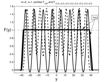
Figure 3. Two patterns, $F_{+20}$ (dashed line) obtained by Cartesian-spherical fibering and $F_{+2,2,+2,2,+2,2,+2,2,+2,2,+2,2,+2,2,+2}$ corresponding to $h=0$; $m=2$, $n=1$.

For $k\gg 1$, these observations can be fixed in a standard asymptotically rigorous manner, which we are not going to do here.

2.3. The origin of countable sequences of solutions: a formal double fibering

Taking into account both changes (2.2) and (2.4), we arrive at the functional

(2.11) $$\hat{E}(h,r,v)\equiv E(h+r(v)v).$$

The relative critical point of (2.11) are given by the system

(2.12) $$\left\{\begin{matrix}\hat{E}_{h}^{\prime}(h,r,v)=0,\\ \hat{E}_{r}^{\prime}(h,r,v)=0,\\ \hat{E}_{v}^{\prime}(h,r,v)=0.\end{matrix}\right.$$

Of course, the first equation is just equivalent to the original one, since

$$\hat{E}_{h}^{\prime}=E^{\prime},$$

so that (2.12) is a formal system comprising the spherical fibering in the $\{r,v\}$-variables, and the original equation. Let us see what kind of conclusions can be derived from this.

The second equation is scalar and gives us necessary smooth branches (under certain hypotheses as above)

(2.13) $$r=r_{*}(h,v)\quad(r_{*}(h,-v)=-r_{*}(h,v)).$$

Then we arrive at the system

(2.14) $$\left\{\begin{matrix}E_{h}^{\prime}(h+r_{*}(h,v)v)=0,\\ E_{v}^{\prime}(h+r_{*}(h,v)v)=0.\end{matrix}\right.$$

The first equation is difficult to handle (possibly more difficult than the original one). However, assume that this can be solved. In view of (2.13), gives an even dependence,

(2.15) $$h=h_{*}(v)\quad(h_{*}(-v)=h_{*}(v)).$$

Finally, we arrive at the even weakly continuous functional for $v$,

(2.16) $$E_{*}(v)\equiv E(h_{*}(v)+r(h_{*}(v),v)v)\quad\mbox{in}\quad{\mathcal{H}}_{0}.$$

This has a countable set of critical point $\{v_{k}\}$, which by fibering method [28], generate critical point of the original functional (2.11).

Therefore, eventually, as $R\to\infty$, we obtain a countable set of necessary critical points

$$(h_{k},w_{k})=((h_{*}(v_{k}),r_{*}(v_{k})v_{k}),\quad k=0,1,2,...\,.$$

The corresponding $F$-patterns are denoted by

$$\{\tilde{F}_{l}\}.$$

The actual general structure of such special solutions remains unclear and needs extra analysis. Currently, we know a little about this and present a few comments only. Using an analogy with the basic Lusternik–Schnirel’man patterns $\{F_{l}\}$ obtained in [11, § 3] for $h=0$, it may be expected that each $\tilde{F}$ is composed from $l\geq 1$ copies of the “elementary” profile $F_{+4}$, i.e.,

$$\tilde{F}_{l}\sim\{F_{+4},-F_{+4},...,(-1)^{l+1}F_{+4}\},$$

with the obvious choice of the corresponding Cartesian approximation $h_{l}(y)$ that is concentrated about equilibria at $\pm 1$ and 0 in between. It is more likely that $\{\tilde{F}_{l}\}$ includes other profiles of the $\{\pm F_{+4},...,\pm F_{+4}\}$-gluing (see [11, § 4] for definitions), or, in particular, can be composed from completely “non-oscillatory” profiles, i.e.,

$$\tilde{F}_{l}=F_{+2l}.$$

3. Problem “Numerics”: patterns in higher-order cases, $m\geq 3$

The main features of the pattern classification by their structure and computed critical values for $m=2$ [11] can be extended to arbitrary $m\geq 3$ in the ODEs (1.5), so we perform this in less detail.

In Figure 4, for the purpose of comparison, we show the first basic pattern $F_{0}(y)$ for $n=1$ in four main cases $m=1$ (the only non-negative profile by the Maximum Principle known from the 1970s [31], [30, Ch. 4]), and $m=2,\,3,\,4$. Next Figure 5 explains oscillatory properties of such $F_{0}(y)$ close to the interface points. It turns out that, for $m=4$, the solutions are most oscillatory, so it is convenient to use this case for further illustrations.

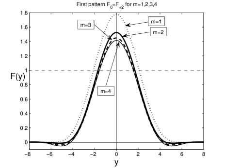
Figure 4. The first solution $F_{0}(y)$ of (1.5), $n=1$, for $m=1,2,3,4$.

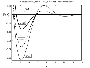
(a) scale $10^{-2}$

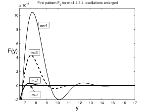
(b) scale $10^{-3}$

Figure 5. Enlarged zero structure of the profile $F_{0}(y)$ for $n=1$ from Figure 4; the linear scale.

In the log-scale, the zero structure of $F_{0}(y)$ near interfaces is shown in Figure 6 for $m=2,3$, and 4 ($n=1$). For $m=4$ and $m=3$, this makes it possible to observe a dozen of “nonlinear” oscillations that well correspond to the already known oscillatory component structure close to interfaces; see [11, § 4]. For the less oscillatory case $m=2$, we observe 4 reliable oscillations up to $10^{-10}$, which is our best accuracy achieved.

Figure 6. Behaviour of $F_{0}(y)$ for $n=1$, for $m=2,3,4$; the log-scale.

The basic countable family satisfying approximate Sturm’s property has the same topology as for $m=2$ [11, § 5], and we do not present such numerical illustrations.

In Figure 7 for $m=3$ and $n=1$, we show the first profiles from the family $\{F_{+2k}\}$, while Figure 8 explains typical structures of $F_{+2,k,+2}\}$ for $m=4$, $n=1$. In Figure 9 for $m=4$ and $n=1$, we show the first profiles from the family $\{F_{+2,k,-2}\}$.

Figure 7. The first seven patterns from the family $\{F_{+2k}\}$; $m=3$ and $n=1$.

Figure 8. The first patterns from the family $\{F_{+2,k,+2}\}$ of the $\{F_{0},F_{0}\}$-interactions; $m=4$ and $n=1$.

(a) profiles

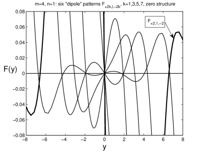
(b) zero structure on $(-8,8)$

Figure 9. The first patterns from the family $\{F_{+2,k,-2}\}$ of the $\{-F_{0},F_{0}\}$-interactions, for $m=4$ and $n=1$: profiles (a), and zero structure around $y=0$ (b).

Finally, in Figure 10, for comparison, we present a complicated pattern for $m=3$ and $4$ (the bold line), $n=1$, with the index

(3.1) $$\sigma=\{-8,3,+4,k,-10,1,+8,l,-12\}.$$

Both numerical experiments were performed starting with the same initial data. As a result, we obtain quite similar patterns, with the only difference that, in (3.1), $k=1$, $l=3$ for $m=3$, and for more oscillatory case $m=4$, the number of zeros increase, so now $k=3$ and $l=5$.

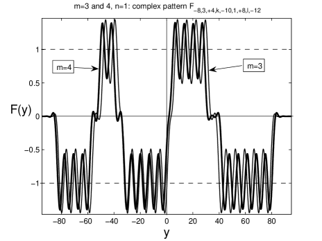
Figure 10. A complicated pattern $F_{\sigma}(y)$ for $m=3,4$ and $n=1$.

4. Problem “Sturm Index”: an homotopy classification of patterns via $\varepsilon$-regularization (analytic-numerical approach)

4.1. Sturm index for second-order ODEs: in need to extension for $m\geq 2$

As we have mentioned, it is well-known that in the second-order case $m=1$, solutions of ODE problems, even in the non-Lipschitz case,

(4.1) $$F^{\prime\prime}=-F+\big{|}F\big{|}^{-\frac{n}{n+1}}F\quad\mbox{in}\quad{\mathbb{R}}$$

obey Sturm’s Theorem on zeros, which is a corollary of the Maximum Principle. Namely, concerning the problem (4.1), each function $F_{l}(y)$ from the basic family has precisely $l$ isolated zeros (sign changes) and $l+1$ non-degenerate extremum points. Therefore, the Sturmian index $I_{l}=l$ of $F_{l}$, as the number of its “transversal zeros”, uniquely specifies any of the basic patterns. This is also equivalent to the Morse index of the corresponding linearized operator. Moreover, the Lusternik–Schnirel’man minimax construction of critical points reveals this zero structure of the minimizers [21, p. 385] that is directly associated with the category [3, § 6.6], or genus [21, § 57], of the sets involved in the variational construction.

For any $m\geq 2$, the Maximum Principle fails, and such a rigorous geometric classification of basic patterns is no longer available in view of existence of oscillatory tails close to both interfaces. Roughly speaking, each profile obtained by the Lusternik–Schnirel’man/fibering approach has infinitely many zeros and extremum points, which makes it impossible to use the above simple geometric characteristics for classification of the patterns as for $m=1$.

Nevertheless, we claim that a Sturmian-type characterization of some (basic) patterns is possible for oscillatory solutions of higher-order ODEs. We will reveal how to attach the Sturmian index to solutions from the basic family $\{F_{l}\}$ in the higher-order case, and also to other families. We consider the ODE case (1.5) for $N=1$, though a similar approach applies to the radial elliptic setting in (1.4), as well as non-radial, where though it is not that well-presented and clear.

We begin with description of higher-order equations admitting a rigorous Sturmian classification of patterns.

4.2. $2m$th-order equations with Sturmian ordering

Consider the following ODE with Dirichlet boundary conditions:

(4.2) $$(-1)^{m+1}F^{(2m)}+F^{3}=0\,\,\,\mbox{in}\,\,\,(-R,R),\quad F=F^{\prime}=...=F^{(m-1)}=0\,\,\,\mbox{at}\,\,\,y=\pm R.$$

This problem is also variational and admits a countable set of solutions $\{F_{l}\}$. Moreover, since the differential operator $(-1)^{m}D_{y}^{2m}$ is an iteration of the positive operator $-D^{2}_{x}$ with the Maximum Principle, according to Elias [7] (see also applications to some nonlinear higher-order eigenvalue problems in [29, 2]), the following result holds:

Proposition 4.1.

The $l$th-solution $F_{l}(y)$ of the problem $(\ref{m1})$ for any $l=0,1,2,...$, has precisely $l$ zeros and $l+1$ extremum points on $(-R,R)$.

In Figures 11 and 12, we present the first solutions of (4.2) for $m=2$ and $m=4$. According to Lusternik–Schnirel’man theory [21, pp. 385-387], each profile $F_{l}$ is obtained by the minimax variational construction (see details in [11, § 3]) on the sets of the category $\rho\geq l+1$.

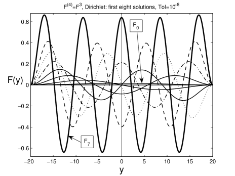
Figure 11. The first eight patterns $F_{l}(y)$ satisfying (4.2) for $m=2$.

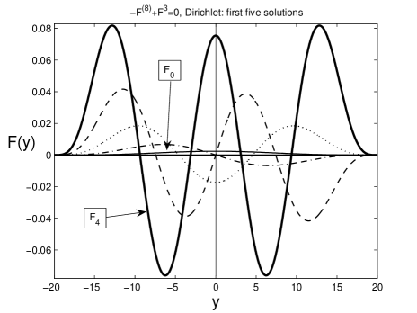
Figure 12. The first five solutions $F_{l}(y)$ of (4.2) for $m=4$.

Remark: convergence to periodic solutions. It is clear from two Figures above (cf. the last boldface profiles) that, for large $l\gg 1$ (actually, already for $l\geq 3$ in both cases), the solutions of the problem $F_{l}(y)$ of (4.2) are close to a periodic structure. Namely, denote by $F_{*}(y)$ a $T_{*}$-periodic solution of the ODE (4.2) in ${\mathbb{R}}$ normalized so that

$$\sup\,|F_{*}(y)|=1.$$

Then, by scaling invariance of the equation,

$$a^{-m}F_{*}\bigl{(}\frac{y}{a}\bigr{)}\quad\mbox{is also a solution in ${\mathbb{R}}$ for any \, $a>0$}.$$

Therefore, for large $l\gg 1$, the following holds:

(4.3) $$F_{l}(y)\approx a_{l}^{-m}F_{*}\bigl{(}\frac{y}{a_{l}}\bigr{)},\quad\mbox{where}\quad a_{l}=\frac{2R}{lT_{*}}\,,$$

and the convergence as $l\to\infty$ is uniform in $y$. Note that the periodic solution $F_{*}$ does not satisfy the Dirichlet boundary conditions at $y=\pm R$, and this creates some boundary layers. It is easy to see that these are of order $o(1)$, i.e., negligible as $l\to\infty$.

4.3. Homotopic connections to the cubic equation

We now introduce the basic one-parametric family of Dirichlet problems in $(-R,R)$ with the operators

(4.4) $${\bf A}_{\varepsilon}(F)\equiv(-1)^{m+1}F^{(2m)}+(1-\varepsilon)\bigl{(}F-\bigl{|}\varepsilon^{2}+F^{2}\bigr{|}^{-\frac{n}{2(n+1)}}F\bigr{)}+\varepsilon F^{3}=0,$$

where $\varepsilon\in[0,1]$. For $\varepsilon=0$, we have the original problem (1.5), while $\varepsilon=1$ gives the above simpler problem (4.2) with all the solutions ordered by Sturm’s index. Notice that, for all $\varepsilon\in(0,1]$, operators (4.4) contain analytic nonlinearities, and the dependence on $\varepsilon$ is also analytic. The only problem of concern is the singular limit $\varepsilon\to 0$.

Our further construction is naturally related to classic theory of homotopy of compact continuous vector fields, [21, § 19]. Denoting by $K(y,\xi)$ the symmetric kernel of the linear operator $(-1)^{m}F^{(2m)}$ with zero Dirichlet conditions, the problems (4.4) can be written in the equivalent integral form

(4.5) $$\Phi_{\varepsilon}(F)\equiv F-(1-\varepsilon)\displaystyle\int K\bigl{(}F-\bigl{|}\varepsilon^{2}+F^{2}\bigr{|}^{-\frac{n}{2(n+1)}}F\bigr{)}-\varepsilon\displaystyle\int KF^{3}=0,$$

where each integral Hammerstein operator is compact and continuous in $L^{2}$ (or suitable $L^{p}$ spaces for $p>2$), [21, p. 83]. Therefore, the function (4.5) for $\varepsilon\in[0,1]$ establishes a deformation of the original vector field

$$\Phi_{0}(F)=F-\displaystyle\int K\bigl{(}F-\bigl{|}F\bigr{|}^{-\frac{n}{n+1}}F\bigr{)}\quad\mbox{into}\quad\Phi_{1}(F)=F-\displaystyle\int KF^{3};$$

see [21, p. 92]. If this deformation is non-singular ($0\not\in\sigma(\Phi_{\varepsilon}^{\prime}(F))$), the two vector fields are homotopic. For convenience, later on we consider the differential form of deformations bearing in mind the necessity to return to the corresponding compact vector fields for any rigorous justification.

Thus, we take an arbitrary solution $F(y)$ of (1.5) with connected symmetric (always achieved by shifting) compact support

$${\rm supp}\,F=[-y_{0},y_{0}].$$

Definition 4.1.

We say that a solution $F(y)$ of $(\ref{S2})$ has Sturm index $l=I_{S}(F)$, if there exists its continuous non-singular deformation, also called a homotopic connection,

(4.6) $$\{F(y;\varepsilon)\,\,\mbox{on}\,\,[-y_{0},y_{0}];\,\varepsilon\in[0,1]\}$$

consisting of critical points (solutions) of the functional for operators $(\ref{e1})$ such that $F(y;0)=F(y)$ and $F(y;1)$ coincides with the solution $F_{l}(y)$ of $(\ref{m1})$.

If, for a given solution $F$ of (1.5), such a non-singular homotopic deformation does not exist, then we say that Sturm’s index $I_{S}(F)$ cannot be attribute to such a function $F$ in principle. In what follows, this nonexistence result can be associated with the fact that, for these solutions, the homotopic connections such as (4.5) (or others) become singular at some saddle-node-type (s-n) bifurcation point $\varepsilon_{\rm s-n}<1$, at which two $\varepsilon$-branches of geometrically similar solutions meet each other.

In general, Sturm’s index can be extended from $\varepsilon=1$ (the ordered cubic problem (4.2)) to $\varepsilon=0$ (the original one) along any continuous analytic branch that can have arbitrary even number of turning s-n points for $\varepsilon\in(0,1)$, and even beyond that. Therefore, in fact we ascribe the same Sturm index $l$ to all profiles belonging to the same analytic branch started for $\varepsilon=1$ at the point $F_{l}$ and ended up at $\varepsilon=0$. In this sense, the nonexistence then means that such a branch in principle is non-extensible to $\varepsilon=0$.

The possibility of bifurcation (branching) points is a key difference between second and higher-order equations. Indeed, for $m=1$, all the (or most interesting) solutions have the index by Sturm’s Theorem on zero sets, while, for $m\geq 2$, there are many others, which principally cannot obey such a simple classification, associated with second-order problems only.

Obviously, along any non-singular homotopic path, the critical points are deformed continuously, which is guaranteed by the Inverse Function Theorem (q.v. e.g. [33, p. 319]). Therefore, our strategy is now to use the Lusternik–Schnirel’man/fibering method for construction of a countable number of branches of different profiles $\{F_{l}\}$, which are ordered by the category of the sets involved. We then apply this for any $\varepsilon\in(0,1)$ in (4.4). Theory of compact integral operators [20, 21, 33] then suggests existence of a countable set of continuous $\varepsilon$-curves of critical points that will continuously attribute the Sturm index from the regular problem (4.2) for $\varepsilon=1$ to the non-Lipschitz one (1.5) for $\varepsilon=0$, provided that these branches are extensible and some of these are not destroyed at saddle-node (or others, even harder) bifurcations in between. Lusternik–Schnirel’man and fibering theory guarantee existence of a countable number of extensible branches. Notice that, ( see [21, p. 387]), to the authors knowledge,

“It is not known whether the Lusternik–Schnirel’man critical
  values are stable.”

On the other hand, there are some definitely stable branches. Therefore, in general, we cannot guarantee that all the Lusternik–Schnirel’man branches are extensible to $\varepsilon=1$. In addition, the proof of the fact that the homotopic path (4.4) (or suitable others) is non-singular, is also a difficult open problem.

Nevertheless, we expect that the stability or non-singularity for (4.4) takes place for our particular problem, and we end up this discussion as follows:

Conjecture 4.1. Each function $F_{l}$ from the basic family $\{F_{l},\,l\geq 0\}$ for $(\ref{S2})$ can be continuously deformed by $(\ref{e1})$ to the corresponding solutions $F_{l}$ of $(\ref{m1})$.

During the course of the inverse $\varepsilon$-deformation from $\varepsilon=1$ to $\varepsilon=0$, the profiles $F_{l}(y;\varepsilon)$ get a finite, depending on $\varepsilon\in(0,1)$, number of oscillations and zeros close to end points $y=\pm R$, and only eventually, at $\varepsilon=0$, this number gets infinity, when the nonlinearity becomes non-Lipschitz and the solutions become compactly supported in $(-R,R)$.

Existence of homotopic connections for basic patterns $F_{l}$. As a typical example, in Figure 13, we present such $\varepsilon$-deformations (4.4) of two profiles, $F_{0}(y)$ (a) and the dipole $F_{1}(y)$ (b) for $n=1$ and $R=10$. The $\varepsilon$-deformation of $F_{2}(y)$ is presented in Figure 14(a) for $n=1$ and $R=10$. A typical corresponding $\varepsilon$-branch of $F_{2}$ is shown in Figure 14(b). All $\varepsilon$-branches of the basic family $\{F_{l}\}$ look quite similarly. Note that these branches can be extended beyond $\varepsilon=1$, and then we observe there the absolute minimum of $\|F\|_{\infty}$ at this value $\varepsilon=1$.

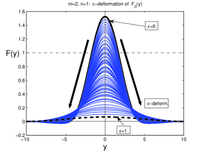
(a) $\varepsilon$-deformation of $F_{0}$, $R=10$

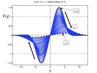
(b) $\varepsilon$-deformation of $F_{1}$, $R=10$

Figure 13. $\varepsilon$-deformation via (4.4) of $F_{0}(y)$ (a) and the 1-dipole profile $F_{1}(y)$ (b).

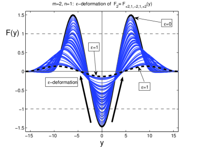
(a) $\varepsilon$-deformation of $F_{2}$, $R=16$

(b) $\varepsilon$-branch of $F_{2}$

Figure 14. The $\varepsilon$-deformation of $F_{2}$ via homotopy (4.4) for $n=1$ (a), and the $\varepsilon$-branch of $F_{2}$ (b).

It is an obvious observation that, by continuity of branches with respect to small changes of nonlinearities, if the homotopic connection as in Figure 14(b) takes place for the basic deformation (4.4) and the branch is infinitely extensible for $\varepsilon>1$, a similar connection $\varepsilon:0\to 1$ can be achieved by other analytic deformations. In this sense, the type of reasonable homotopic deformations is not that crucial; cf. Proposition 4.2 below establishing an analogous non-homotopy conclusion.

Nonexistence of $\varepsilon$-connections and saddle-node bifurcations. We now deal with other families of non-basic patterns obtained in Section 2 by an extra preliminary Cartesian $h$-approximation. We then introduce their total generalized Sturm index, which should include the number of oscillations about the non-trivial equilibria $\pm 1$ defined by the structure of $h(y)$; see Section 7 for an alternative approach to the generalized index via a spatial $R$-compression of profiles.

Then, a homotopic $\varepsilon$-deformation of these patterns to those of the equation (4.2) with monotone nonlinearity is not possible in principle. We claim that, on the $\{\varepsilon,F\}$-plane of the global bifurcation diagram, their solution branches appear in standard saddle-node bifurcations that occur for $\varepsilon<1$, i.e., these branches do not admit extensions up to the simpler ODEs (4.2).

Using the enhanced numerics with Tols=$10^{-4}$ and the step $\Delta\varepsilon=10^{-3}$, we show the $\varepsilon$-deformation of two non-basic profiles given in Figure 15,

(4.7) $$F_{+4}(y)\quad\mbox{and}\quad F_{+2,2,+2}(y),$$

which have similar geometric shapes, with the equal numbers of four intersections with the equilibrium $+1$. This detailed $\varepsilon$-deformation via (4.4) for $n=1$, of $F_{+4}(y)$ and $F_{2}\equiv F_{+2,2,+2}(y)$ is shown in Figure 15(a) and (b) in [13] (these are too big, 5.3 and 2.33 MB, to be presented in arXiv). The $\varepsilon$-deformations of these two profiles turns out to stop at the same saddle-node bifurcation at $\varepsilon=\varepsilon_{\rm s-n}=0.709...\,.$

In Figure 16, we show the corresponding $\varepsilon$-bifurcation diagram with a saddle-node bifurcation at

(4.8) $$\framebox{$\varepsilon_{\rm s-n}=0.709...\quad(F_{+4},\,\,\,R=14),$}$$

at which the branch of $F_{+4}$ and the branch of $F_{+2,2,+2}$ meet each other. For convenience, in Figure 16, we also draw neighbouring global branches of the basic patterns $F_{4}$ and $F_{2}=F_{+2,-2,+2}$ (existing for all $\varepsilon\in[0,1]$), to which the corresponding branches jump being extended above the bifurcation values (4.8).

It turns out that a neighbouring branch of the basic pattern $F_{4}$ exists for $\varepsilon>\varepsilon_{\rm s-n}$, while the neighbouring basic branch is that of $F_{3}=F_{+2,1,-2,1,+2}$. Being extended numerically for $\varepsilon>\varepsilon_{\rm s-n}$, the $\varepsilon$-branches of profiles (4.7) jump to these basic $\varepsilon$-branches.

Such a branching at $\varepsilon=\varepsilon_{\rm s-n}$ means that the two profiles (4.7) belong to the same family, both having the generalized Sturm index $\sigma_{\rm min}=+4$.

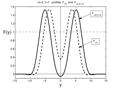
Figure 15. Patterns $F_{+4}$ and $F_{+2,2,+2}$ have similar geometric shapes and appear simultaneously at the s-n bifurcation at (4.8); $m=2$, $N=n=1$.

It is not difficult to choose other pairs of patterns $F$ with similar geometries, which have to be originated at saddle-node bifurcations for $\varepsilon<1$. For instance, these are $F_{+2k}$ and $F_{+2,2,+2,2,...,2,+2}$, with $k$ single patterns $\sim+F_{0}$ gluing together.

\psfrag{||F||}{$\|F\|_{\infty}$}\psfrag{e}{$\varepsilon$}\psfrag{t2}{$t_{2}$}\psfrag{F222}{$F_{+2,2,+2}$}\psfrag{F+4}{$F_{+4}$}\psfrag{F2}{$F_{2}$}\psfrag{final-time profile}{final-time profile}\psfrag{F4}{$F_{4}$}\psfrag{x}{$x$}\psfrag{0<t1<t2<t3<t4}{$0<t_{1}<t_{2}<t_{3}<t_{4}$}\psfrag{0}{$0$}\psfrag{l}{$l$}\psfrag{-l}{$-l$}\includegraphics[scale={0.5}]{bbbifN.eps}

Figure 16. The $\varepsilon$-branches of $F_{+4}$ and $F_{+2,2,+2}$ cannot be extended from $\varepsilon=0$ via (4.4) to $\varepsilon=1$ and meet at a saddle-node bifurcation at $\varepsilon_{\rm s-n}=0.709...$ . The neighbouring branches of $F_{4}$ and $F_{2}$, which are detected in Figure 15(a), (b) in [13] are also shown.

For example, Figure 17 shows the $\varepsilon$-deformation of (see Figure 18(a))

(4.9) $$F_{+6}(y)\quad\mbox{and}\quad F_{+2,2,+2,2,+2}(y).$$

In Figure 18(b), we show the corresponding bifurcation diagram. Notice that the corresponding s-n bifurcation point,

$$\framebox{$\varepsilon_{\rm s-n}=0.700...\quad(F_{+6},\,\,\,R=20),$}$$

is rather close to (4.8) for $F_{+4}$ (notice different lengths $R$). For $F_{+8}$ and $F_{+2,2+2,2,+2,2+2,2}$ shown in Figure 19 for the same $R=20$, it is different,

$$\framebox{$\varepsilon_{\rm s-n}=0.52...\quad(F_{+8},\,\,\,R=20).$}$$

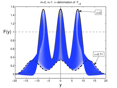
(a) $\varepsilon$-deformation of $F_{+6}$, $R=20$

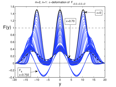
(b) $\varepsilon$-deformation of $F_{+2,2,+2,2,+2}$, $R=20$

Figure 17. $\varepsilon$-deformation via (4.4) for $m=2$, $n=1$, of $F_{+6}(y)$ (a) and $F_{+2,2,+2,2,+2}(y)$ stops at the same saddle-node bifurcation at $\varepsilon=\varepsilon_{\rm s-n}=0.700...$ .

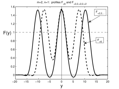
(a) profiles $F_{+6}$ and $F_{+2,2,+2,2,+2,2}$

(b) $\varepsilon$-bifurcation diagram

Figure 18. $m=2$, $n=1$: profiles $F_{+6}(y)$ and $F_{+2,2,+2,2,+2}(y)$ (a); bifurcation diagram (b).

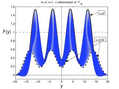
Figure 19. $\varepsilon$-deformation via (4.4) for $m=2$, $n=1$, of $F_{+8}(y)$ is possible until $\varepsilon_{\rm s-n}=0.52...$.

Meanwhile, for convenience, we present the following simple conclusion showing that nonexistence of the homotopic path (4.5) actually means nonexistence of any analytic non-singular connections. In particular, this indicates that the geometric type of the branching in Figure 16 is generic.

Proposition 4.2.

Let, for a given solution $F$ of $(\ref{S2})$, the basic deformation $(\ref{e1int})$ have a singular point at some $\varepsilon_{\rm s-n}<1$, where two continuous branches of two patterns originated at $\varepsilon=0$ meet each other and hence cannot be continued up to $\varepsilon=1$. Then any analytic deformation of these patterns generating the functional path $(\ref{epath})$ ends up at a singular point for some $\varepsilon\in(0,1)$.

In other words, other analytic deformations cannot move the s-n point into the set $\{\varepsilon>1\}$ just by continuity.

Proof. Without loss of generality, we assume that the corresponding critical values and the points $\{F_{l}\}$ of the cubic problem (4.2) are non-singular (by changing $R$ if necessary). Since any continuous deformation of the basic path will continuously (and analytically) deform the branches, the existence of a homotopic path would mean that at some instant, the s-n point of the branches will touch the vertical line $\varepsilon=1$. At this moment, we would create a singular value for the analytic cubic problem (4.2), a contradiction. ∎

Numerically, we have observed a curious phenomenon: in a left-hand neighbourhood of the saddle-node bifurcation at $\varepsilon=\varepsilon_{\rm s-n}$, the profiles keep only essential non-monotonicity features and loose all intersections with zero, so become non-oscillatory near transversal zeros. Therefore, according to such an $\varepsilon$-deformation to saddle-node bifurcations, the number of intersections with the trivial equilibrium 0 at $\varepsilon=0$ should not be taken into account in the generalized Strum index. In this sense, the complicated profiles on Figure 10 have the following generalized Sturm index:

$$\sigma_{\rm min}=\{-8,+4,-10,+8-12\};$$

see Section 7 for details and more mathematics. One can “split” this index to get equivalent pairs of profiles originated at some $\varepsilon_{\rm s-n}<1$.

4.4. Homotopic connection to linear eigenvalue problems

This is an alternative way to ascribe Sturm’s index to basic patterns $\{F_{l}$}. Modifying the nonlinearity in the approximation (4.4), we consider the following operator family (watch the last term):

(4.10) $$\hat{\bf A}_{\varepsilon}(F)=(-1)^{m+1}F^{(2m)}+(1-\varepsilon)\bigl{(}F-\bigl{|}\varepsilon^{2}+F^{2}\bigr{|}^{-\frac{n}{2(n+1)}}|F|^{\varepsilon}F\bigr{)},\quad\varepsilon\in[0,1].$$

As usual, by the actual homotopic connection we mean the corresponding vector fields composed of compact integral operators. Then, from (4.10) at $\varepsilon=1$, we obtain the linear operator

$$\hat{\bf A}_{1}(F)=(-1)^{m+1}F^{(2m)}.$$

On the other hand, for any $\varepsilon>0$, the linearized operator at 0 is very simple,

(4.11) $$\hat{\bf A}_{1}^{\prime}(0)=(-1)^{m+1}D^{2m}_{y}+(1-\varepsilon)I,\quad\varepsilon\in(0,1].$$

Denoting by $\sigma=\{-\lambda_{l}>0,\,l\geq 0\}$ the eigenvalues of the negative operator $(-1)^{m}D^{2m}_{y}$, it follows that [21, Ch. 8]

$$\varepsilon_{l}=1-\lambda_{l}\quad\mbox{for any}\quad l\geq 0$$

are subcritical bifurcation points, where the necessary $\varepsilon$-branches appear. Along those branches that are originated at $\varepsilon_{l}>0$, for $\varepsilon=0$ we obtain our nonlinear eigenfunctions $\{F_{l}\}$, which thus inherit the Sturmian structure and the index from the eigenfunction $\psi_{l}$ (it has precisely $l$ zeros and $l+1$ extrema points; see Section 6) that governs the pattern for $\varepsilon\approx\varepsilon_{l}^{-}$. We continue developing such an $\varepsilon$-deformation approach to linear eigenvalue problems in Section 6 devoted to ODEs with analytic nonlinearities.

5. Problem with “fast diffusion” : extinction and blow-up phenomenon in the Dirichlet setting

Here, using typical concavity-like techniques, we prove that finite-time extinction for the PDE (1.13) is a generic property of their bounded weak solutions. Firstly, we study this phenomenon in a bounded domain in ${\mathbb{R}}^{N}$ with homogeneous Dirichlet boundary conditions. Secondly, for the Cauchy problem, possible (and rather complicated) types of extinction patterns will be revealed in the next Section 6 by using our separate variable similarity patterns.

5.1. Extinction for some nonlinear parabolic problems of higher order: main result

Let $\Omega$ be a bounded sufficiently smooth domain in ${\mathbb{R}}^{N}$. Taking the original equation (1.13) and setting, as usual,

$$|u|^{n}u=v\quad\Longrightarrow\quad u=|v|^{-\frac{n}{n+1}}\,v,\quad\mbox{where}\quad-\frac{n}{n+1}>0\,\,\,\mbox{for}\,\,\,n\in(-1,0),$$

we arrive at the following initial boundary value problem:

(5.1) $$\left\{\begin{aligned} &\mbox{$\frac{\partial}{\partial t}\psi(v)$}=(-1)^{m+1}\Delta^{m}v+v&&\mbox{ in }Q=\Omega\times{\mathbb{R}}_{+},\\ &v=Dv=\ldots=D^{m-1}v=0&&\mbox{ on }\partial\Omega\times{\mathbb{R}}_{+},\\ &v(x,0)=v_{0}(x)&&\mbox{ in }\Omega,\end{aligned}\right.$$

where $v_{0}$ is an initial function from an appropriate space to be specified. Here, the only nonlinearity is $\psi(v)=|v|^{-\frac{n}{n+1}}v$. We examine the problem (5.1) in the “native” energy Sobolev space.

Let us introduce the following functionals associated with the operators in (5.1):

$$\Phi(t) :=\mbox{$\frac{1}{2}\displaystyle\int_{\Omega}|v(t,x)|^{\frac{n+2}{n+1}}\,{\mathrm{d}}x,$}\vskip 3.0pt plus 1.0pt minus 1.0pt$$

$$E(t) :=\mbox{$-\displaystyle\int_{\Omega}|\tilde{D}^{m}v(t,x)|^{2}\,{\mathrm{d}}x-\displaystyle\int_{\Omega}v^{2}\,{\mathrm{d}}x.$}$$

Lemma 5.1.

There holds

$$\Phi^{\prime}(t)=\frac{n+2}{2}E(t).$$

The proof follows from simple calculations. The main result on extinction in (5.1) is as follows:

Theorem 5.1.

(Extinction) For given nontrivial initial data, denote:

$$\Phi(0) =\frac{1}{2}\displaystyle\int_{\Omega}|v_{0}|^{\frac{n+2}{n+1}}\,{\mathrm{d}}x>0,$$

$$E(0) =\mbox{$-\displaystyle\int_{\Omega}|\tilde{D}^{m}v_{0}|^{2}\,{\mathrm{d}}x-\displaystyle\int_{\Omega}v_{0}^{2}\,{\mathrm{d}}x<0.$}$$

Then

(5.2) $$\Phi(t)\leq\Phi(0)\frac{1}{\left(1-\frac{t}{T}\right)^{\frac{n+2}{n}}}=\left(1-\frac{t}{T}\right)^{\left|\frac{n+2}{n}\right|}\Phi(0)\to 0\,\,\,\mbox{as}\,\,\,t\to T^{-},$$

with

$$T:=\frac{n+2}{n}\frac{\Phi(0)}{\Phi^{\prime}(0)}=\frac{2}{n}\frac{\Phi(0)}{E(0)}>0.$$

The proof is divided into several steps.

5.2. The first energy relation

Multiplying the equation in (5.1) by $v$ and integrating by parts over $\Omega\times(0,T)$ by taking into account the boundary conditions, we obtain

(5.3) $$\frac{1}{n+2}\displaystyle\int_{\Omega}\left.|v|^{\frac{n+2}{n+1}}\right|_{0}^{T}\,{\mathrm{d}}x=-\iint_{\Omega}|\tilde{D}^{m}v|^{2}\,\,{\mathrm{d}}x\,{\mathrm{d}}t-\iint_{\Omega}v^{2}\,\,{\mathrm{d}}x\,{\mathrm{d}}t.$$

5.3. The second energy relation

Multiplying the equation in (5.1) by $v_{t}$ and again integrating by parts over $\Omega\times(0,T)$ by using the boundary conditions, we obtain

(5.4) $$\iint_{\Omega}\psi^{\prime}(v)v_{t}^{2}\,{\mathrm{d}}x\,{\mathrm{d}}t=\left.\left(-\frac{1}{2}\displaystyle\int_{\Omega}|\tilde{D}^{m}v|^{2}\,{\mathrm{d}}x-\frac{1}{2}\displaystyle\int_{\Omega}v^{2}\,{\mathrm{d}}x\right)\right|_{0}^{T}.$$

5.4. Connection (a main point)

Denote

$$\tilde{U}(t):=-\displaystyle\int_{\Omega}|\tilde{D}^{m}v|^{2}\,{\mathrm{d}}x-\displaystyle\int_{\Omega}|v|^{2}\,{\mathrm{d}}x, \tilde{V}(t):=\frac{1}{n+2}\displaystyle\int_{\Omega}|v|^{\frac{n+2}{n+1}}\,{\mathrm{d}}x.$$   

Then the identity (5.3) reads

(5.5) $$\mbox{$\left.\tilde{V}(t)\right|_{0}^{T}=\displaystyle\int_{0}^{T}\tilde{U}(t){\mathrm{d}}t,$}\quad\mbox{or equivalently},\quad\mbox{$\displaystyle\frac{d\tilde{V}}{{\mathrm{d}}t}=\tilde{U}(t).$}$$

Analogously, it follows from (5.4) that

(5.6) $$\frac{d\tilde{U}}{{\mathrm{d}}t}=\frac{2}{n+1}\displaystyle\int_{\Omega}|v|^{-\frac{n}{n+1}}(v_{t})^{2}\,\,{\mathrm{d}}x.$$

5.5. The main (crucial) relation

We deduce from (5.5) and (5.6) that

(5.7) $$\frac{d^{2}\tilde{V}}{{\mathrm{d}}t^{2}}=\frac{d\tilde{U}}{{\mathrm{d}}t}=\frac{2}{n+1}\displaystyle\int_{\Omega}|v|^{-\frac{n}{n+1}}(v_{t})^{2}\,{\mathrm{d}}x.$$

Next, by the definition of $\tilde{V}$, we have

$$\tilde{V}_{tt}=\displaystyle\frac{1}{(n+1)^{2}}\displaystyle\int_{\Omega}|V|^{-\frac{n}{n+1}}(v_{t})^{2}\,{\mathrm{d}}x+\frac{1}{n+1}\displaystyle\int_{\Omega}|v|^{-\frac{n}{n+1}}vv_{tt}\,{\mathrm{d}}x.$$

Thus, equation (5.7) takes the form

(5.8) $$\int_{\Omega}|v|^{-\frac{n}{n+1}}vv_{tt}\,{\mathrm{d}}x=\frac{2n+1}{n+1}\displaystyle\int_{\Omega}|v|^{-\frac{n}{n+1}}(v_{t})^{2}\,\,{\mathrm{d}}x.$$

5.6. Replacement

We introduce a new function $z=z(x,t)$ by the formula

$$v=|z|^{\frac{n}{n+2}}z.$$

Then equation (5.8) reads

(5.9) $$\int_{\Omega}zz_{tt}\,\,{\mathrm{d}}x=c_{n}\displaystyle\int_{\Omega}(z_{t})^{2}\,\,{\mathrm{d}}x,\quad\mbox{with \,\, $\displaystyle c_{n}=\frac{3n+2}{n+2}$}.$$

5.7. Fourier analysis of equation (5.9)

Let $(e_{k})_{k\in\mathbf{N}}$ be a complete orthonormal system in $L^{2}(\Omega)$. Then we have

$$z(x,t) =\mbox{ $\sum_{k=1}^{\infty}z_{k}(t)e_{k}(x),$}$$

$$z_{t}(x,t) =\mbox{ $\sum_{k=1}^{\infty}z_{k}^{\prime}(t)e_{k}(x),$}$$

$$z_{tt}(x,t) =\mbox{ $\sum_{k=1}^{\infty}z_{k}^{\prime\prime}(t)e_{k}(x).$}$$

Let

$$\Phi(t)=\frac{1}{2}\displaystyle\int_{\Omega}z^{2}(x,t)\,{\mathrm{d}}x=\frac{1}{2}\sum_{k=1}^{\infty}z_{k}(t)^{2},$$

so that

(5.10) $$\Phi^{\prime}(t)=\frac{1}{2}\frac{\mathrm{d}}{{\mathrm{d}}t}\displaystyle\int_{\Omega}|z|^{2}\,\,{\mathrm{d}}x=\displaystyle\int_{\Omega}zz_{t}\,\,{\mathrm{d}}x=\sum_{k=1}^{\infty}z_{k}z_{k}^{\prime},$$

and hence, by Holder’s inequality,

$$(\Phi^{\prime})^{2}\leq\left(\sum_{k=1}^{\infty}z_{k}^{2}\right)\left(\sum_{k=1}^{\infty}z_{k}^{\prime 2}\right)=2\Phi\sum_{k=1}^{\infty}z_{k}^{\prime 2}.$$

In Fourier coefficients, equation (5.9) takes the form

(5.11) $$\sum_{k=1}^{\infty}zz_{k}^{\prime\prime}=c_{n}\sum_{k=1}^{\infty}z_{k}^{\prime 2}.$$

On the other hand, in terms of the function $\Phi$, we have

$$\Phi^{\prime\prime}=\displaystyle\sum_{k=1}^{\infty}z_{k}z_{k}^{\prime\prime}+\sum_{k=1}^{\infty}z_{k}^{\prime 2}.$$

Consequently, equation (5.11) takes the form

$$\Phi^{\prime\prime}-\displaystyle\sum_{k=1}^{\infty}z_{k}^{\prime 2}=c_{n}\sum_{k=1}^{\infty}z_{k}^{\prime 2}.$$

Therefore,

$$\Phi^{\prime\prime}=(1+c_{n})\sum_{k=1}^{\infty}z_{k}^{\prime 2}\geq\frac{1+c_{n}}{2}\,\displaystyle\frac{(\Phi^{\prime})^{2}}{\Phi},$$   i.e.,

(5.12) $$\Phi\Phi^{\prime\prime}\geq k_{n}\Phi^{\prime 2},\quad\mbox{where}$$

$$k_{n}:=\frac{1+c_{n}}{2}=\frac{2(n+1)}{n+2}<1\quad(\mbox{for }n\in(-2,0)).$$

5.8. Extinction: the proof

For the analysis of an ordinary differential inequality appeared, we can use various approaches. For the case where $\Phi^{\prime}<0$, we apply the standard approach. Namely, we divide inequality (5.12) by $\Phi^{\prime}$. Then we obtain

$$\frac{\Phi^{\prime\prime}}{\Phi^{\prime}}\leq k_{n}\frac{\Phi^{\prime}}{\Phi}.$$

From here, it then follows that

$$\Phi^{\prime}(t)\leq C_{1}\Phi^{k_{n}}(t),$$

with $\displaystyle C_{1}=\frac{\Phi^{\prime}(0)}{\Phi^{k_{n}}(0)}<0$ for $E(0)<0$.

This inequality implies the result of the main theorem. For the proof, it suffices to replace our new variables with the original function $v$ by the formula

$$\Phi(t)=\frac{1}{2}\displaystyle\int_{\Omega}z^{2}(x,t)\,{\mathrm{d}}x=\frac{1}{2}\displaystyle\int_{\Omega}|v|^{\frac{n+2}{n+1}}\,\,{\mathrm{d}}x$$

so that

$$\Phi^{\prime}(t)=\displaystyle\frac{d\Phi}{{\mathrm{d}}t}=\displaystyle\int_{\Omega}zz_{t}\,\,{\mathrm{d}}x =\mbox{$\displaystyle\frac{1}{2}\,\frac{n+2}{n+1}\displaystyle\int_{\Omega}\psi(v)v_{t}\,\,{\mathrm{d}}x$}$$

$$=\mbox{$\displaystyle\frac{1}{2}\,\frac{n+2}{n+1}\displaystyle\int_{\Omega}\frac{\psi(v)}{\psi^{\prime}(v)}\psi^{\prime}(v)v_{t}\,\,{\mathrm{d}}x$}$$

$$=\mbox{$\displaystyle\frac{1}{2}\,\frac{n+2}{n+1}\displaystyle\int_{\Omega}(n+1)v\psi(v)_{t}\,\,{\mathrm{d}}x$}$$

$$=\mbox{$\displaystyle\frac{n+2}{2}\displaystyle\int_{\Omega}v\psi(v)_{t}\,\,{\mathrm{d}}x$}$$

$$=\mbox{$\displaystyle\frac{n+2}{2}E(v),$}$$

where

$$E(v)=-\displaystyle\int_{\Omega}|\tilde{D}^{m}v|^{2}\,\,{\mathrm{d}}x-\displaystyle\int_{\Omega}v^{2}\,\,{\mathrm{d}}x.$$

This completes the proof of Theorem 5.1.

5.9. A diversion to blow-up for $n>0$

By using the same computations as above we can prove the following blow-up result for the original equation (1.1).

Theorem 5.2.

(Blow-up) Suppose that $n>0$ in $(\ref{111})$. Let

$$\Phi(0) =\frac{1}{2}\int_{\Omega}|v_{0}|^{\frac{n+2}{n+1}}\,{\mathrm{d}}x>0,$$

$$E(0) =-\int_{\Omega}|\tilde{D}^{m}v_{0}|^{2}\,{\mathrm{d}}x+\int_{\Omega}v_{0}^{2}\,{\mathrm{d}}x>0.$$

Then

$$\Phi(t)\geq\Phi(0)\frac{1}{\left(1-t/T\right)^{\frac{n+2}{n}}}$$

with

$$T:=\frac{n+2}{n}\frac{\Phi(0)}{\Phi^{\prime}(0)}=\frac{2}{n}\frac{\Phi(0)}{E(0)}.$$

5.10. Blow-up: the proof

In this case, following the computations as in (5.11), we obtain,

$$\Phi^{\prime\prime}-\displaystyle\sum_{k=1}^{\infty}z_{k}^{\prime 2}=c_{n}\sum_{k=1}^{\infty}z_{k}^{\prime 2}.$$

Therefore,

$$\Phi^{\prime\prime}=(1+c_{n})\sum_{k=1}^{\infty}z_{k}^{\prime 2}\geq\frac{1+c_{n}}{2\Phi}\Phi^{\prime 2},$$

i.e.,

(5.13) $$\Phi\Phi^{\prime\prime}\geq k_{n}\Phi^{\prime 2},$$

where

$$k_{n}:=\frac{1+c_{n}}{2}=2\frac{n+1}{n+2}>1\quad(\mbox{for }n>0).$$

For the case where $\Phi^{\prime}>0$, we apply the standard approach.

Namely, we divide inequality (5.13) by $\Phi^{\prime}$. Then we obtain

$$\frac{\Phi^{\prime\prime}}{\Phi^{\prime}}\geq k_{n}\frac{\Phi^{\prime}}{\Phi}.$$

From here, it follows that

$$\Phi^{\prime}(t)\geq C_{1}\Phi(t)^{k_{n}}$$

with $C_{1}=\dfrac{\Phi^{\prime}(0)}{\Phi(0)^{k_{n}}}>0$ for $E(0)>0$.

This inequality implies the result of the main theorem.

Indeed, it is enough to replace our new variables with the original function $v$ by the formula

$$\Phi(t)=\frac{1}{2}\int_{\Omega}z(t,x)^{2}\,\,{\mathrm{d}}x=\frac{1}{2}\int_{\Omega}|v|^{\frac{n+2}{n+1}}\,\,{\mathrm{d}}x$$

and

$$\Phi^{\prime}(t)=\frac{{\mathrm{d}}\Phi}{{\mathrm{d}}t}=\int_{\Omega}zz_{t}\,\,{\mathrm{d}}x =\frac{1}{2}\cdot\frac{n+2}{n+1}\int_{\Omega}\psi(v)v_{t}\,\,{\mathrm{d}}x$$

$$=\frac{1}{2}\cdot\frac{n+2}{n+1}\int_{\Omega}\frac{\psi(v)}{\psi^{\prime}(v)}\psi^{\prime}(v)v_{t}\,\,{\mathrm{d}}x$$

$$=\frac{1}{2}\cdot\frac{n+2}{n+1}\int_{\Omega}(n+1)v\psi(v)_{t}\,\,{\mathrm{d}}x$$

$$=\frac{n+2}{2}\int_{\Omega}v\psi(v)_{t}\,\,{\mathrm{d}}x$$

$$=\frac{n+2}{2}E(v),$$

where

$$E(v)=-\int_{\Omega}\left(|\tilde{D}^{m}v|^{2}+v^{2}\right)\,{\mathrm{d}}x.$$

6. Problem “fast diffusion”: existence, multiplicity, etc.

6.1. Oscillatory ODEs with analytic nonlinearities from fast diffusion

Here we consider another ODE model (1.7), and without loss of generality, we mainly restrict to $m=2$. We show that (1.7) provides us with similar countable families of various patterns. Moreover, we claim that the solution set of (1.7) is equivalent to that obtained earlier for non-Lipschitz nonlinearities. Indeed, solutions $F(y)$ of (1.7) are not compactly supported and exhibit oscillatory exponential decay at infinity governed by the linearized operator

(6.1) $$F^{(4)}=-F+...\quad\Longrightarrow\quad F(y)\sim{\mathrm{e}}^{-\frac{y}{\sqrt{2}}}\cos\bigl{(}\frac{\sqrt{3}}{2}y+c\bigr{)},\quad y\to+\infty.$$

6.2. Patterns

Figures 20 and 21 show a few typical patterns, which we are already familiar with. It is important to notice that, in Figure 20, by watching the behaviour of small negative solutions close to the origin $y=0$, there are two different patterns that can be classified as $F_{+2,2,+2}$, and the second one is denoted by $F^{*}_{+2,2,+2}$. This shows again that the number of intersections with equilibria $\pm 1$ and 0 are not enough for a complete pattern description (in fact, this underlines that a homotopy approach using the hodograph plane is not applicable to equations such as (1.16)). It is seen there that $F^{*}_{+2,2,+2}(y)$ exhibit more non-monotone structure for $y\in(-4,4)$ than $F_{+2,2,+2}(y)$, so that the derivative $F^{*^{\prime}}_{+2,2,+2}(y)$ has there 3 zeros therein, while $F^{\prime}_{+2,2,+2}(y)$ has just one at $y=0$. Thus, these two patterns can be distinguished by the number of zeros of their derivatives, but, by the same reasons, we do not think that counting internal zeros of the pairs $\{F(y),\,F^{\prime}(y)\}$ can help to create any rigorous Sturmian-like classification of such patterns.

In Figure 22, we present typical complicated patterns for the problem (1.7), which remind similar “multi-hump” structures obtained above in Figure 10.

Note that, in view of the fast exponential decay (6.1), it is difficult to observe by standard numerical methods that, unlike the previous problem, the profiles in Figure 22 are not compactly supported. Note that, for $n>0$, we succeeded in the logarithmic scale, by taking small regularization parameter and tolerances $\sim 10^{-12}$, to reveal the difference between the linearized zero-behaviour (as in (6.1)) and the nonlinear one at the interface as $y\to y_{0}^{+}$ of the type ($\varphi(s)$ is the oscillatory component; see Figure 6 and [11, 12, § 4])

(6.2) $$F(y)=(y-y_{0})^{\gamma}\varphi(s),\quad\mbox{where}\quad s=\ln(y-y_{0})\quad\mbox{and}\quad\gamma=\frac{2m(n+1)}{n}>2m.$$

For $n<0$, there are no “nonlinear zeros”, but there exists an infinite number of linearized ones given by (6.1), first dozens of which can be easily observed numerically.

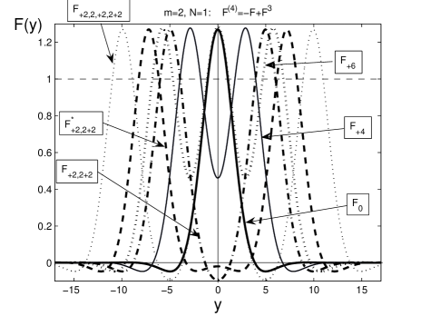
Figure 20. Various solutions of the ODE (1.7): positively dominant patterns.

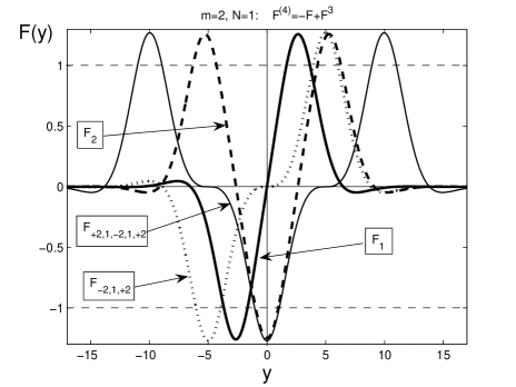
Figure 21. Various solutions of the ODE (1.7): essentially changing sign patterns.

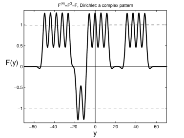
(a) $F_{+10,1,-4,+6,4,+8}$

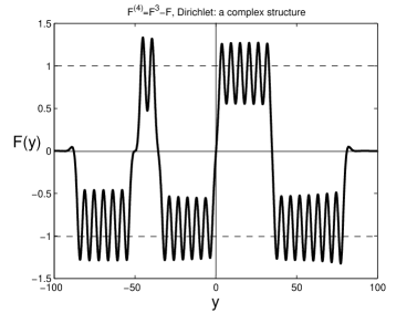
(b) $F_{-12,1,+4,1,-12,1,+12,1,-16}$

Figure 22. Examples of complicated patterns of the ODE (1.7).

6.3. Application of Lusternik–Schnirel’man and fibering theory

Obviously, the ODE (1.7) (or the elliptic problem in (1.16)) possesses the variational setting in $(-R,R)$ (or $B_{R}$), to which the same fibering version of Lusternik–Schnirel’man theory applies, as in [11, 12, § 3]. This gives a countable family of basic patterns $\{F_{l}\}$ for both the ODE and the elliptic PDE. Introducing the preliminary $h$-approximation of patterns makes it possible to reconstruct other families of more complicated geometric structure. Since $F_{l}$ are not compactly supported, we always assume fixing $R=R(l)\gg 1$ for $l\gg 1$. The solutions in ${\mathbb{R}}$ (${\mathbb{R}}^{N}$) are then obtained by passing to the limit $l\to\infty$. We do not stress the attention to such a compactness procedure that assumes deriving some uniform bounds independent of $l$. On the other hand, in view of the known exponential decay of all the solutions, the variational statement in the whole space ${\mathbb{R}}^{N}$ is also an option; see [26]. We now present brief comments.

The functional is

(6.3) $${E}(F)=\frac{1}{2}\displaystyle\int|\tilde{D}^{m}F|^{2}+\frac{1}{2}\displaystyle\int F^{2}-\frac{1}{4}\,\displaystyle\int F^{4}.$$

The spherical fibering [11, 12, § 3] with $v$ belonging to the unit sphere,

(6.4) $$F=r(v)v,\quad\mbox{where}\,\,\,v\in{\mathcal{H}}_{0}=\bigl{\{}H_{0}(v)\equiv\displaystyle\int|\tilde{D}^{m}v|^{2}+\displaystyle\int v^{2}=1\bigr{\}},$$

leads to the functional

(6.5) $$H(r,v)=\frac{1}{2}\,r^{2}-\frac{1}{4}\,r^{4}\displaystyle\int v^{4}.$$

This attains the absolute maximum at

(6.6) $$H^{\prime}_{r}\equiv r-r^{3}\displaystyle\int v^{4}=0\,\,\Longrightarrow\,\,r_{0}(v)=\frac{1}{\sqrt{\displaystyle\int v^{4}}},$$

at which $H(r_{0}(v),v)=\frac{1}{2\sqrt{\displaystyle\int v^{4}}}.$ This defines the positive homogeneous convex functional

(6.7) $$\tilde{H}(v)=\bigl{[}\frac{1}{2H(r_{0}(v),v)}\bigr{]}^{2}\equiv\displaystyle\int v^{4}.$$

Here Lusternik–Schnirel’man theory applies in its classic form [21, p. 387] giving a countable set $\{c_{k}\}$ of critical values and points denoted by $\{v_{k}\}$ (see full details in [11, 12, § 3]):

(6.8) $$c_{k}=\sup_{{\mathcal{F}}\in{\mathcal{M}}_{k}}\,\,\inf_{v\in{\mathcal{F}}}\,\,\displaystyle\int v^{4}.$$

Now the sequence of critical values is decreasing,

(6.9) $$c_{1}\geq c_{2}\geq...\geq c_{k}\geq c_{k+1}\geq...\,.$$

For each $v_{k}$ (a solution $F_{k}$), the critical values are given by

(6.10) $$v=CF\in{\mathcal{H}}_{0}\quad\Longrightarrow\quad c_{F}\equiv\tilde{H}(v)=\frac{\displaystyle\int F^{4}}{\left(\displaystyle\int|\tilde{D}^{m}F|^{2}+\displaystyle\int F^{2}\right)^{2}}\,.$$

For all the patterns shown in Figures 20 and 21, these values (Lusternik–Schnirel’man critical or not) are presented in Table 1. As usual, this table makes it possible to detect the Lusternik–Schnirel’man critical points that deliver critical values (6.8) for each genus. We then again claim that the basic patterns $\{F_{l}\}$ deliver all the Lusternik–Schnirel’man critical values (6.8) with $k=l+1$.

Recall the Formal Rule of Composition (FRC) from [11, 12, § 5]: performing maximization of $\tilde{H}(v)$ of any $(k-1)$-dimensional manifold ${\mathcal{F}}\in{\mathcal{M}}_{k}$,

(6.11) the Lusternik–Schnirel’man point $$F_{k-1}(y)$$ is obtained by minimizing all internal tails and zeros,

i.e., making the minimal number of internal transversal zeros between single structures. Then (6.11) also applies, since by the same reason diminishing a small tail between two $F_{0}$-structures will increase the corresponding value $c_{F}$ in (6.10).

Table 1. Critical values of $\tilde{H}(v)=\frac{\displaystyle\int F^{4}}{\left(\displaystyle\int|\tilde{D}^{m}F|^{2}+\displaystyle\int F^{2}\right)^{2}}$

$F$	$c_{F}$
$F_{0}$	$0.2033...=c_{1}$
$F_{1}$	$0.1080...=c_{2}$
$F_{+2,2,+2}$	$0.1019...$
$\tilde{F}_{+2,2,+2}$	$0.1017...$
$\tilde{F}_{-2,1,+2}$	$0.1014...$
$F_{+4}$	$0.0961...$
$F_{2}$	$0.0736...=c_{3}$
$F_{+2,2,+2,2,+2}$	$0.0680...$
$\tilde{F}_{+2,1,-2,1,+2}$	$0.0675...$
$F_{+6}$	$0.0629...$

6.4. Homotopic connections with Sturm-ordered linear eigenvalue problems

An extra advantage of the problem (1.7) is that the homotopic connections of basic patterns can be revealed easier. Namely, as above, we consider the ODE (1.7) in $(-R,R)$ with sufficiently large $R>0$ to see the first $l$ patterns which are still exponentially small for $y\approx\pm R$. Consider the following homotopic path with the operators:

(6.12) $${\bf A}_{\varepsilon}(F)\equiv F^{(4)}+\varepsilon F-F^{3}=0.$$

Consider the corresponding linearized operator:

(6.13) $${\bf A}_{\varepsilon}^{\prime}(0)=D_{y}^{4}+\varepsilon I.$$

Let $\sigma(D_{y}^{4})=\{\lambda_{l}>0,\,l\geq 0\}$ be the discrete spectrum of simple eigenvalues of $D_{y}^{4}>0$ in $L^{2}((-R,R))$ with the Dirichlet boundary conditions. The orthonormal eigenfunctions $\{\psi_{l}\}$ satisfy Sturm’s zero property; we again refer to [7] for most general results.

By classic bifurcation theory [21, p. 391], for such variational problems,

$$\varepsilon_{l}=-\lambda_{l}<0\quad\mbox{for}\quad l=0,1,2,...$$

are bifurcation points, so there exists a countable number of branches emanating from these points (but we take into account the first ones). In order to identify the type of bifurcations, in a standard manner, setting $\varepsilon=\varepsilon_{l}+s$ for $|s|$ small and

$$F=C\psi_{l}+w,\quad\mbox{where}\quad w\bot\psi_{l},$$

substituting into (6.12) and multiplying by $\psi_{l}$ yields

$$s=C^{2}(s)\displaystyle\int\psi_{l}^{4}+...>0\quad\Longrightarrow\quad s>0\,\,\,\mbox{and}\,\,\,C(s)=\pm\sqrt{\frac{s}{\displaystyle\int\psi_{l}^{4}}}+...\,.$$

Hence, at $\varepsilon=\varepsilon_{l}$, there appear two branches with the equations

$$F_{l}(y)=\pm\sqrt{\frac{\varepsilon-\varepsilon_{l}}{\displaystyle\int\psi_{l}^{4}}}\,\,\psi_{l}(y)+...\quad\mbox{for}\quad\varepsilon>\varepsilon_{l}.$$

Therefore, all the bifurcations are pitchfork and are supercritical, i.e., two symmetric branches are initiated at $\varepsilon=\varepsilon_{l}^{+}$; see Figure 23(a), where we construct numerically the first positive $\varepsilon$-branch of $F_{0}$ of the $\varepsilon$-bifurcation diagram and show that this branch is extensible up to the necessary value $\varepsilon=1$, and even up to $\varepsilon\sim 10^{2}$ (b), and further.

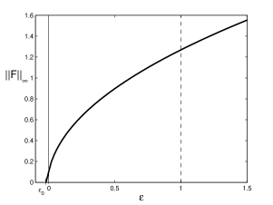
(a) $\varepsilon\sim 1$

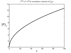
(b) $\varepsilon\sim 100$

Figure 23. The monotone $\varepsilon$-branch of profile $F_{0}$ via homotopy (4.4) on different scales; $\varepsilon\in(-\varepsilon_{0},1.5)$ (a) and $\epsilon\in(0,100)$ (b).

It follows that all the branches are originated at $\varepsilon_{l}<0$, so being continued up to $\varepsilon=1$, give the original equation (1.7). The questions of global continuation of branches are classic in nonlinear variational theory; see [3, § 6.7C]. The global behaviour of bifurcation branches for $2m$th-order ODEs with analysis of possible types of end-points is addressed in [2]. These results hardly apply to the equation (4.4) with non-coercive operators admitting solutions of changing sign near boundary points.

The existence of a turning point of the given branch in this real self-adjoint case, i.e., of a saddle-node bifurcation, assumes that there exists an eigenvalue (say, simple)

$$0\in\sigma({\bf A}_{\varepsilon}^{\prime}(F)),\quad\mbox{i.e.,}\quad\exists\,\,\phi_{0}:\,\,\phi_{0}^{(4)}+\varepsilon\phi_{0}-3F^{2}\phi_{0}=0,$$

where $\phi_{0}$ is an eigenfunction of ${\bf A}_{\varepsilon}^{\prime}(F)$ satisfying the Dirichlet conditions $\phi_{0}=\phi_{0}^{\prime}=0$ at $y=\pm R$. For a moment, we digress from our difficult ODEs and consider simpler models with known bifurcation diagrams.

Remark 1: on turning saddle-node bifurcation points of positive solutions. Such turning points do exist for equations with other nonlinearities and another dependence on $\varepsilon$, e.g.,

(6.14) $$(-1)^{m}F^{(2m)}=\varepsilon{\mathrm{e}}^{F}\quad\mbox{or}\quad(-1)^{m}F^{(2m)}=\varepsilon(1+F^{3})\,\,\,(F\geq 0),$$

with Dirichlet boundary conditions at $\pm R$. Existence of two different branches of solutions (they are positive by [7]) for all small $\varepsilon>0$ is established by the fibering method as in [11, 12, § 3].

On the other hand, for $\varepsilon\gg 1$, positive solutions of (6.14) are obviously not possible. This is easily seen by multiplying the first equation in (6.14) by the first eigenfunction $\psi_{0}>0$ with the eigenvalue $\lambda_{0}>0$ of the positive operator $(-1)^{m}D_{y}^{2m}$. This gives for the first Fourier coefficient $C_{0}=\displaystyle\int F\psi_{0}$ the following inequality:

(6.15) $$\lambda_{0}C_{0}=\varepsilon\displaystyle\int{\mathrm{e}}^{F}\psi_{0}\equiv\varepsilon\|\psi_{0}\|_{1}\displaystyle\int{\mathrm{e}}^{F}\frac{\psi_{0}}{\|\psi_{0}\|_{1}}\geq\varepsilon\|\psi_{0}\|_{1}\,\,{\mathrm{e}}^{\displaystyle\int F\frac{\psi_{0}}{\|\psi_{0}\|_{1}}}=\varepsilon\|\psi_{0}\|_{1}\,\,{\mathrm{e}}^{\frac{C_{0}}{\|\psi_{0}\|_{1}}}.$$

At the last stage we have used Jensen’s inequality for the convex function ${\mathrm{e}}^{F}$. One can see that the resulting inequality in (6.15),

$$\lambda_{0}C_{0}\geq\varepsilon\|\psi_{0}\|_{1}\,\,{\mathrm{e}}^{\frac{C_{0}}{\|\psi_{0}\|_{1}}},$$

does not have a solution $C_{0}>0$ for all $\varepsilon\gg 1$, meaning nonexistence.

By standard theory of compact integral Uryson–Hammerstein operators [20, 21] and branching theory [33], the solutions of (6.14) detected for small $\varepsilon>0$ comprise two continuous branches, which must end up at a saddle-node bifurcation point (no other bifurcations are possible) at some

$$\varepsilon=\varepsilon_{\rm s-n}>0.$$

In Figure 24, the global bifurcation diagram is presented for the quadratic equation,

(6.16) $$F^{(4)}=\varepsilon(1+F^{2})\quad\mbox{on \, $(-1,1)$},\quad\mbox{where}\quad\framebox{$\varepsilon_{\rm s-n}=14.91...$}\,.$$

The upper branch blows-up to $+\infty$ as $\varepsilon\to 0^{+}$, while the lower one vanishes. See [19] for a different approach to bifurcation analysis for such fourth-order ODEs.

\psfrag{||F||}{$\|F\|_{\infty}$}\psfrag{e}{$\varepsilon$}\psfrag{t2}{$t_{2}$}\psfrag{t3}{$t_{3}$}\psfrag{t4}{$t_{4}$}\psfrag{v(x,t-)}{$v(x,T^{-})$}\psfrag{final-time profile}{final-time profile}\psfrag{tapp1}{$t\approx 1^{-}$}\psfrag{x}{$x$}\psfrag{0<t1<t2<t3<t4}{$0<t_{1}<t_{2}<t_{3}<t_{4}$}\psfrag{0}{$0$}\psfrag{l}{$l$}\psfrag{-l}{$-l$}\includegraphics[scale={0.5}]{BD1.eps}

Figure 24. The bifurcation diagram for (6.16).

We return to the equation (6.12). Nonexistence of such saddle-node bifurcation points for the ODEs (6.12) is a difficult open problem. Numerically, we have got a strong evidence that the first branches are strictly monotone without turning points; see Figure 23(b), where the first branch is extended up to $\varepsilon=100$.

On the other hand, it is easy to check by the fibering approach that (6.12) has a countable set of solutions for arbitrarily large $\varepsilon>0$, which are also identified as continuous curves by nonlinear compact operator theory. Hence, there are infinitely many branches of basic patterns that are unboundently extensible in $\varepsilon$. We then conclude that at $\varepsilon=1$ all these branches are available. Hence, at $\varepsilon=1$, the corresponding solutions $F_{l}$ of (1.7) inherit their Sturm index from eigenfunctions $\psi_{l}$ that occur at $\varepsilon=\varepsilon_{l}^{+}$.

Of course, we can use the alternative homotopy approach. Figure 23(a) shows that the $\varepsilon$-branches are well-defined at $\varepsilon=0$, where we obtain the simpler equation

$$-F^{(4)}+F^{3}=0$$

that, as in (4.2), admits Sturm’s classification of all the patterns.

Remark 2: explicit global monotone $\varepsilon$-bifurcation branches for a non-local nonlinearity. Computations of branches are straightforward for the following non-local equation with the analytic cubic nonlinearity (cf. (6.12)):

(6.17) $$F^{(4)}=-\varepsilon F+\bigl{(}\displaystyle\int F^{2}\bigr{)}F\quad\mbox{in}\quad(-R,R).$$

Then the solutions

$$F_{l}(y)=\pm\sqrt{\lambda_{l}+\varepsilon}\,\,\psi_{l}(y)\quad\mbox{for}\quad l=0,1,2,...$$

are originated at $\varepsilon_{l}=-\lambda_{l}^{+}$, and the branches have the geometric form as in Figure 23.

7. Problem “Sturm Index”: using $R$-compression

Consider again for a while the simplest non-Lipschitz ODE for $m=2$:

(7.1) $$F^{(4)}=F-\big{|}F\big{|}^{-\frac{n}{n+1}}F\quad\mbox{in}\,\,\,{\mathbb{R}}.$$

As we have seen, the oscillatory character of the solutions close to interfaces, finite or infinite, causes some difficulties in determining the actual (generalized) Sturm index of the patterns defined as the number of certain oscillations, which are “dominant” zeros (or extrema) points about 0. Oscillations about non-trivial equilibria $\pm 1$ are clear and do not exhibit such difficulties, though sometimes it is rather hard to distinguish these classes of non-monotonicities. The main problem of concern is that how to distinguish the “dominant” non-monotonicities and “small” non-dominant ones related to asymptotic oscillations close to interfaces, which are almost the same for all the patterns; cf. [11, 12, § 4] for the non-Lipschitz nonlinearity and (6.1) for the analytic one (1.7).

As we know, in the CP for the PDEs involved, it is enough to pose the Dirichlet problem for (1.5) on sufficiently large intervals $(-R,R)$, so one does not need to take infinite length $R=+\infty$. Let is concentrate on the case $m=2$,

(7.2) $$F^{(4)}=F-\big{|}F\big{|}^{-\frac{n}{n+1}}F\quad\mbox{in}\,\,\,(-R,R),$$

with Dirichlet conditions at the end-points $y=\pm R$. Given a compactly supported pattern

(7.3) $$F(y)=F_{\sigma}(y),\quad\mbox{with multiindex}\quad\sigma=\{\sigma_{1},\sigma_{2},\sigma_{3},...,\sigma_{l}\}\quad\big{(}{\rm supp}\,F_{\sigma}\subset(-R,R)\big{)},$$

we perform its $R$-compression, i.e., start to decrease $R$ observing a continuous deformation of the corresponding profile $F(y;R)$ until the minimally possible value

$$R=R_{\rm min}>2R_{*}>0\quad(\mbox{$R_{*}$ is defined in \cite[cite]{[\@@bibref{}{GMPSob,GMPSobIarX}{}{}, \S~{}3]}}).$$

Let $\sigma_{\rm min}$ be the multiindex of $F(y;R_{\rm min})$, if this profile is bounded. If not, we mean the index $F(y;R_{\rm min}^{+})$ calculated for profiles with $R\approx R_{\rm min}^{+}$. As usual, $\sigma_{\rm min}$ reflects the sequence of intersection numbers with equilibria $\pm 1$, without taking into account those with 0, which are, actually, nonexistent; see below. There is a direct relation to Definition 4.1 to be explained later on:

Definition 7.1.

Given a compactly supported solution $(\ref{pp1})$ of $(\ref{4.3R})$, by its generalized Sturm index we mean the multiindex $\sigma_{\rm min}$ obtained by the $R$-compression.

Two cases of $R$-compression are distinguished:

(i) As $R\to R_{\rm min}^{+}$, the profile $F(y;R)$ gets unbounded and achieves a clear geometric form with $l$ extrema. Then we say that this $l$ is precisely the Sturm index $l=I_{\rm S}$ of the functions $F$ on this $R$-branch. As usual, we claim that such an index $l$ can be attributed to the basic family $\{F_{l}\}$ only.

(ii) There exists a finite limit $F(y;R_{\rm min})$. Then the only generalized Sturm index can be defined as a characterization of its geometric structure with fixed numbers of intersections with equilibria $\pm 1$.

In Figure 25, we present some numerical results of the $R$-compression of the profile $F_{0}$ (a) (interfaces become non-oscillatory already for $R\sim 5$, $\sigma_{\rm min}=\{+2\}$ as expected, i.e., with no essential “transversal” zeros and a single maximum) and $F_{+2,2,+2}$ (b) (non-oscillatory interfaces for $R\sim 10$, $\sigma_{\rm min}=\{+4\}$, no essential zeros and three extrema). In (b), by dotted lines, we denote some other profiles that also appear for such $R\approx R_{\rm min}^{+}$. These belong to other branches of solutions of (7.2).

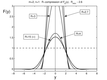
(a) $F_{0}$

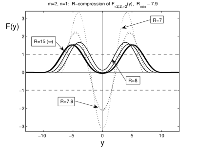
(b) $F_{+2,2,+2}$

Figure 25. The $R$-compression of solutions of the ODE (7.1) for $n=1$; $F_{0}$ (a) and $F_{+2,2,+2}$ (b).

In Figure 26, we show the $R$-compression of a different profile, $F_{+4}$, with a similar structure. Note that, in Figures 26 and 25(b), the profiles for $R=8$ coincide. This again confirms (cf. Figure 16 for an $\varepsilon$-deformation of those) that these profiles belong to two branches originated at a supercritical saddle-node $R$-bifurcation at $R_{\rm min}\sim 7.9$. Observe in Figure 26 other dotted profiles of a similar geometric structure that exist close to $R_{\rm min}^{+}$ and indeed correspond to the third basic pattern $F_{2}=F_{+2,-2,+2}$. The intriguing global $R$-bifurcation diagram with saddle-node bifurcations turns out to be similar to that observed in Section 4 by the $\varepsilon$-homotopy approach; see more explanations below.

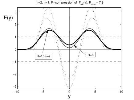
Figure 26. The $R$-compression of the solution $F_{+4}$ of the ODE (7.1) for $n=1$.

We do not need to develop more consistent theory of $R$-compression in view of the following simple comment:

$\varepsilon$-homotopy and $R$-compression can be equivalent. For simplicity, consider the analytic ODE problem (6.12) on $(-R,R)$, where we perform the scaling

$$F(y)=\sqrt{\varepsilon}\,V(z),\quad y=\varepsilon^{\frac{1}{4}}z\quad(\varepsilon>0).$$

Then $\varepsilon$ is scaled out from the ODE and enters the interval, where the problem is posed:

(7.4) $$V^{(4)}=-V+V^{3}\quad\mbox{on}\quad\bigl{(}-\varepsilon^{\frac{1}{4}}R,\varepsilon^{\frac{1}{4}}R\bigr{)}.$$

Therefore, in this particular case, the $\varepsilon$-deformation of the equation (6.12) is equivalent to the $R$-compression for (7.4) as $\varepsilon>0$ decreases. So these two approaches to Sturm’s index of highly oscillatory structures are essentially equivalent and hence lead to the same results. In particular, this explains the striking phenomenon (observed in Section 4) that, at saddle-node bifurcations, the profiles lose all their oscillations about zero.

8. On essentially quasilinear extensions: gradient diffusivity

8.1. Variational problems with $p$-Laplacian operators

For simplicity, we consider PDEs (1.20) in 1D, where these have simpler forms,

(8.1) $$\begin{matrix}{\bf(I)}\quad u_{t}=-(|u_{xx}|^{n}u_{xx})_{xx}+|u|^{n}u\quad(\mbox{parabolic}),\,\,\vskip 3.0pt plus 1.0pt minus 1.0pt\vskip 3.0pt plus 1.0pt minus 1.0pt\\ {\bf(II)}\quad u_{tt}=-(|u_{xx}|^{n}u_{xx})_{xx}+|u|^{n}u\quad(\mbox{hyperbolic}),\vskip 3.0pt plus 1.0pt minus 1.0pt\vskip 3.0pt plus 1.0pt minus 1.0pt\\ {\bf(III)}\quad u_{t}=-(|u_{xx}|^{n}u_{xx})_{xxx}+(|u|^{n}u)_{x}\quad(\mbox{NDE}).\quad\,\,\end{matrix}$$

For the reaction-diffusion PDE (I), the blow-up solutions are the same, (1.2), with

(8.2) $$\frac{1}{n}\,f=-(|f^{\prime\prime}|^{n}f^{\prime\prime})^{\prime\prime}+|f|^{n}f.$$

Using the scaling yields the basic quasilinear ODE:

(8.3) $$f=n^{-\frac{1}{n}}F\quad\Longrightarrow\quad\framebox{$-(|F^{\prime\prime}|^{n}F^{\prime\prime})^{\prime\prime}+|F|^{n}F-F=0\quad\mbox{in}\quad{\mathbb{R}}.$}$$

For the hyperbolic PDE (II), we construct the blow-up patterns (1.9), where the same scaling yields (8.3). Finally, for the NDE (III), the TW compacton

$$u_{\rm c}(x,t)=f(x-\lambda t),\quad\mbox{with}\quad\lambda=-1,$$

directly leads to the ODE in (8.3).

In all the three cases, for the $N$-dimensional PDEs (1.20), we arrive at the elliptic PDE,

(8.4) $$\framebox{$-\Delta(|\Delta F|^{n}\Delta F)+|F|^{n}F-F=0\quad\mbox{in}\quad{\mathbb{R}},$}$$

admitting variational formulation in $L^{2}({\mathbb{R}}^{N})$ with the potential (cf. (2.1))

(8.5) $$E(F)=-\frac{1}{n+2}\,\displaystyle\int_{{\mathbb{R}}^{N}}|\Delta F|^{n+2}+\frac{1}{n+2}\,\displaystyle\int_{{\mathbb{R}}^{N}}|F|^{n+2}-\frac{1}{2}\,\displaystyle\int_{{\mathbb{R}}^{N}}F^{2}.$$

Then the same Lusternik–Schnirel’man/fibering approaches can be applied to get a countable basic family of compactly supported solutions and next discover other countable sets of blow-up patterns, etc. We claim that the most of principal results obtained above for the semilinear elliptic problems can be extended to the quasilinear one (8.4), though some local (e.g., oscillatory structures of solutions near finite interfaces) or global aspects of the behaviour of patterns are more complicated. Some local oscillatory properties of solutions of changing sign are discussed in [15, pp. 246–249] and [9]. All these problems admit more general $2m$th-order extensions along the same lines as usual.

8.2. Related non-variational problems: branching “from” potential results

Finally, let us mention that there exists a variety of slightly changed PDEs (I)–(II), which, on exact blow-up solutions, reduce to elliptic or ODE problems that are principally non-variational. A systematic study of such problems with non-coercive, non-monotone, and non-potential operators touches another wide area of open mathematical problems.

For instance, consider a reaction-diffusion equation with the nonlinearity from (1.21),

(8.6) $$u_{t}=-\Delta(|\Delta u|^{n}\Delta u)+|u|^{p}u,\quad\mbox{where}\quad p>n>0.$$

The similarity blow-up solutions are not separable as in (1.2) and have the form

(8.7) $$u_{\rm S}(x,t)=(T-t)^{-\frac{1}{p}}f(y),\quad y=x/(T-t)^{\beta},\quad\mbox{where}\quad\beta=\frac{p-n}{2p(n+2)}>0.$$

Substituting (8.7) into (8.6) yields the following elliptic equation:

(8.8) $$\framebox{$-\Delta(|\Delta f|^{n}\Delta f)-\beta y\cdot\nabla f-\frac{1}{p}\,f+|f|^{p}f=0\quad\mbox{in \,\, ${\mathbb{R}}^{N}$}.$}$$

For $p=n$ we have $\beta=0$, so that (8.8) reduces to the above variational equation (8.4).

We claim that, for $p\not=n$, the differential operator in (8.8) is not variational (even for $n=0$; see [17, § 7]), so all above techniques fail. Nevertheless, we also claim that the present variational analysis can and does play a role for such problems. Namely, the variational problem (8.4) for $p=n$ has the following meaning:

(8.9) $$\framebox{$\begin{matrix}\mbox{potential eq. (\ref{el111}) initiates {\em branching} at $p=n$ of solutions of non-potential}\vskip 3.0pt plus 1.0pt minus 1.0pt\\ \mbox{eq. (\ref{par3}) from the Lusternik--Schnirel'man/fibering patterns $\{F_{l}\}$.}\end{matrix}$}$$

Such ideas well-correspond to classic branching theory; see Vainberg–Trenogin [33]. Therefore, we expect that still, even not being variational,

(8.10) $$\mbox{(\ref{par3}) admits arbitrarily large number of solutions for $p\approx n^{+}$}.$$

Here we should assume that $p$ is sufficiently close to $n^{+}$, since, as usual, global continuation of local bifurcation branches is a difficult open problem. Note that, for $p>n$, solutions of (8.8) are not compactly supported in general (for $p\in(0,n]$ these are). Applications of such a branching approach to (8.8) with $N=1$ and $p>n$ and $p<n$ are given in [9].

Branching phenomena for such nonlinear and degenerate operators as in (8.8) are not standard and demand a lot of work; see e.g., [1], where thin film operators have been dealt with. On the other hand, the $p$-branching analysis in the semilinear case $n=0$ for equations such as (8.8) uses spectral theory of non self-adjoint operators and is easier; see examples in [5, 10, 17].

In other words, precisely (8.9) is the actual role that variational problems can play for describing finite or countable sets of solutions of principally non-variational ones, so that the results such as (8.10) can be inherited from a suitable potential asymptotic setting. Finding such a variational problem by introducing a parameter as a good approximation of the given non-potential one can be rather tricky, though for equations like (8.8), this looks natural and straightforward.

References

- [1] P. Álvarez-Caudevilla and V.A. Galaktionov, Local bifurcation-branching analysis of global and “blow-up” patterns for a fourth-order thin film equation, submitted (arXiv:1009.5864).
- [2] R. Bari and B. Rynne, Solution curves and exact multiplicity results for th order boundary value problems, J. Math. Anal. Appl., 292 (2004), 17–22.
- [3] M. Berger, Nonlinearity and Functional Analysis, Acad. Press, New York, 1977.
- [4] H. Brezis and F. Brawder, Partial Differential Equations in the 20th Century, Adv. in Math., 135 (1998), 76–144.
- [5] C.J. Budd, V.A. Galaktionov, and J.F. Williams, Self-similar blow-up in higher-order semilinear parabolic equations, SIAM J. Appl. Math., 64 (2004), 1775–1809.
- [6] C.V. Coffman, Uniqueness of the ground state for and a variational characterization of other solutions, Arch. Rat. Mech. Anal., 46 (1972), 81–95.
- [7] U. Elias, Eigenvalue problems for the equation , J. Differ. Equat., 29 (1978), 28–57.
- [8] V.A. Galaktionov, On interfaces and oscillatory solutions of higher-order semilinear parabolic equations with non-Lipschitz nonlinearities, Stud. Appl. Math., 117 (2006), 353–389.
- [9] V.A. Galaktionov, Three types of self-similar blow-up for the fourth-order -Laplacian equation with source, J. Comp. Appl. Math., 223 (2009), 326–355 (arXiv:0903.0981).
- [10] V.A. Galaktinov and P.J. Harwin, Non-uniqueness and global similarity solutions for a higher-order semilinear parabolic equation, Nonlinearity, 18 (2005), 717–746.
- [11] V.A. Galaktionov, E. Mitidieri, and S.I. Pohozaev, Variational approach to complicated similarity solutions of higher-order nonlinear evolution equations of parabolic, hyperbolic, and nonlinear dispersion types, In: Sobolev Spaces in Mathematics. II, Appl. Anal. and Part. Differ. Equat., Series: Int. Math. Ser., Vol. 9, V. Maz’ya Ed., Springer, New York, 2009 (an extended version in arXiv:0902.1425).
- [12] V.A. Galaktionov, E. Mitidieri, and S.I. Pohozaev, Variational approach to complicated similarity solutions of higher-order nonlinear PDEs. I, arXiv:0902.1425.
- [13] V.A. Galaktionov, E. Mitidieri, and S.I. Pohozaev, Variational approach to complicated similarity solutions of higher-order nonlinear PDEs. II, Nonl. Anal: RWA, DOI: 10.1016/j.nonrwa.2011.03.001.
- [14] V.A. Galaktionov and S.I. Pohozaev, Third-order nonlinear dispersive equations: shocks, rarefaction, and blow-up waves, Comput. Math. Math. Phys., 48 (2008), 1784–1810 (arXiv:0902.0253).
- [15] V.A. Galaktionov and S.R. Svirshchevskii, Exact Solutions and Invariant Subspaces of Nonlinear Partial Differential Equations in Mechanics and Physics, ChapmanHall/CRC, Boca Raton, Florida, 2007.
- [16] V.A. Galaktionov and J.L. Vázquez, A Stability Technique for Evolution Partial Differential Equations. A Dynamical Systems Approach, Progr. in Nonl. Differ. Equat. and their Appl., 56, Birkhäuser Boston, Inc., MA, 2004.
- [17] V.A. Galaktionov and J.F. Williams, On very singular similarity solutions of a higher-order semilinear parabolic equation, Nonlinearity, 17 (2004), 1075–1099.
- [18] W.D. Kalies, J. Kwapisz, J.B. VandenBerg, and R.C.A.M. VanderVorst, Homotopy classes for stable periodic and chaotic patterns in fourth-order Hamiltonian systems, Commun. Math. Phys., 214 (2000), 573–592.
- [19] P. Korman, Uniqueness and exact multiplicity of solutions for a class of fourth-order semilinear problems, Proc. Roy. Soc. Edinburgh, Sect. A, 134 (2004), 179–190.
- [20] M.A. Krasnosel’skii, Topological Methods in the Theory of Nonlinear Integral Equations, Pergamon Press, Oxford/Paris, 1964.
- [21] M.A. Krasnosel’skii and P.P. Zabreiko, Geometrical Methods of Nonlinear Analysis, Springer-Verlag, Berlin/Tokyo, 1984.
- [22] F. Merle and P. Raphael, On a sharp lower bound on the blow-up rate for the critical nonlinear Schrödinger equation, J. Amer. Math. Soc., 19 (2005), 37–90.
- [23] F. Merle and P. Raphael, The blow-up dynamics and upper bound on the blow-up rate for critical nonlinear Schrödinger equation, Ann. Math., 161 (2005), 157–222.
- [24] F. Merle and P. Raphael, Profiles and quantization of the blow-up mass for critical nonlinear Schrödinger equation, Comm. Math. Phys., 253 (2005), 675–704.
- [25] E. Mitidieri and S.I. Pohozaev, A priori estimates and the absence of solutions of nonlinear partial differential equations and inequalities., Proc. Steklov Inst. Math., Vol. 234, Intern. Acad. Publ. Comp. Nauka/Interperiodica, Moscow, 2001.
- [26] L.A. Peletier and W.C. Troy, Spatial Patterns: Higher Order Models in Physics and Mechanics, Birkhäuser, Boston/Berlin, 2001.
- [27] S.I. Pohozaev, On an approach to nonlinear equations, Soviet Math. Dokl., 20 (1979), 912–916.
- [28] S.I. Pohozaev, The fibering method in nonlinear variational problems, Pitman Research Notes in Math., Vol. 365, Pitman, 1997, pp. 35–88.
- [29] B. Rynn, Global bifurcation for th-order boundary value problems and infinitely many solutions of superlinear problems, J. Differ. Equat., 188 (2003), 461–472.
- [30] A.A. Samarskii, V.A. Galaktionov, S.P. Kurdyumov, and A.P. Mikhailov, Blow-up in Quasilinear Parabolic Equations, Walter de Gruyter, Berlin/New York, 1995.
- [31] A.A. Samarskii, N.V. Zmitrenko, S.P. Kurdyumov, and A.P. Mikhailov, Thermal structures and fundamental length in a medium with non-linear heat conduction and volumetric heat sources, Soviet Phys. Dokl., 21 (1976), 141–143.
- [32] A.E. Shishkov, Dead cores and instantaneous compactification of the supports of energy solutions of quasilinear parabolic equations of arbitrary order, Sbornik: Math., 190 (1999), 1843–1869.
- [33] M.A. Vainberg and V.A. Trenogin, Theory of Branching of Solutions of Non-Linear Equations, Noordhoff Int. Publ., Leiden, 1974.
- [34] J.B. Van Den Berg and R.C. Vandervorst, Stable patterns for fourth-order parabolic equations, Duke Math. J., 115 (2002), 513–558.