Conserved directed percolation: exact quasistationary distribution of small systems and Monte Carlo simulations

Abstract

We study symmetric sleepy random walkers, a model exhibiting an absorbing-state phase transition in the conserved directed percolation (CDP) universality class. Unlike most examples of this class studied previously, this model possesses a continuously variable control parameter, facilitating analysis of critical properties. We study the model using two complementary approaches: analysis of the numerically exact quasistationary (QS) probability distribution on rings of up to $22$ sites, and Monte Carlo simulation of systems of up to $32000$ sites. The resulting estimates for critical exponents $\beta$, $\beta/\nu_{\perp}$, and $z$, and the moment ratio $m_{211}=\langle\rho^{2}\rangle/\langle\rho\rangle^{2}$ ($\rho$ is the activity density), based on finite-size scaling at the critical point, are in agreement with previous results for the CDP universality class. We find, however, that the approach to the QS regime is characterized by a different value of the dynamic exponent $z$ than found in the QS regime.

I Introduction

Over the last several decades, phase transitions between an active and an absorbing state have attracted great interest in statistical physics and related fields Hinrichsen ; livrodickman ; lubeck ; geza . More recently, experiments on such transitions have been performed takeuchi ; bacterias ; pine1 . As in equilibrium, continuous phase transitions to an absorbing state can be grouped into universality classes lubeck ; geza . Two classes that have received much attention are directed percolation (DP) and conserved directed percolation (CDP), exemplified, respectively, by the contact process harris and the stochastic conserved sandpile (conserved Manna model) manna ; manna1d . While the former class is well characterized, and there is a clear, consistent picture of the scaling behavior, the critical exponents of CDP have not been determined to high precision, and there are suggestions of violations of scaling. Thus it is of interest to study further examples of this class, and to apply new methods of analysis to such models. Absorbing-state transitions have been studied via mean-field theory, series expansion livrodickman , renormalization group padrao , perturbation theory pertubacao and numerical simulation. Recently, an analysis based on the exact (numerical) determination of the quasistationary (QS) probability distribution was proposed and applied to models in the DP class exact sol .

In this paper we study sleepy random walkers (SRW), a Markov process defined on a lattice, belonging to the CDP universality class, using exact (numerical) analysis of the quasistationary (QS) probability distribution and Monte Carlo simulation. The former approach furnishes quite accurate predictions for the contact process; a preliminary application to a model in the CDP class yielded less encouraging results, due in part to the small system sizes accessible exact sol . The smaller number of configurations (for a given lattice size and particle density) in the SRW model allows us to study somewhat larger systems, leading to improved results in the QS analysis. We study the model in extensive Monte Carlo simulations as well, in efforts to better characterize CDP critical behavior. A closely related model, activated random walkers (ARW), was introduced in vladas ; in this case there is no restriction on the number of walkers per site. In vladas the principal emphasis was on asymmetric ARW (hopping in one direction only); some preliminary evidence for CDP-like behavior of the symmetric version was also reported.

The balance of this paper is organized as follows. In Sec. II we define the model and its behavior in mean-field theory. In Sec. III we describe how exact QS analysis is applied to the model and present the associated results on critical behavior. We report our simulation results in Sec. IV, and in Sec. V we present a summary of our findings.

II Model

The SRW model is defined on a $d$-dimensional lattice of $L^{d}$ sites with periodic boundary conditions. Each site $i$ of the lattice may be in one of three states: empty ($\sigma_{i}=0$), occupied by an active particle ($\sigma_{i}=1$), or by an inactive particle ($\sigma_{i}=-1$). Multiple occupancy is forbidden. Active particles attempt to hop, at unit rate, to a nearest-neighbor site. In a hopping move the target site is chosen with uniform probability on the set of nearest neighbors, and the move is accepted if and only if the target site is vacant. Transitions from $\sigma_{i}=1$ (active) to $\sigma_{i}=-1$ (inactive) occur at a rate of $\lambda$, called the sleeping rate, independent of the states of the other sites. Inactive particles cannot hop. A transition from $\sigma_{i}=-1$ to $\sigma_{i}=1$ occurs when an active neighbor attempts to jump to site $i$. In this case, the particle that attempted to hop returns to its original site, but the particle that was sleeping is activated. Evidently this Markovian dynamics conserves the number of particles. Here we consider initial configurations in which $N$ particles (all active) are distributed randomly amongst the sites, respecting the prohibition of multiple occupancy. (In the ARW model vladas the number of particles per site is unrestricted but only an isolated particle can sleep.)

Let $N_{a}$ denote the number of active particles; any configuration with $N_{a}=0$ is absorbing. Thus we define the order parameter as $\rho\equiv N_{a}/N$, the fraction of active particles. There are two control parameters, the sleeping rate $\lambda$ and the particle density $\zeta=N/L^{d}$. For $\zeta<1$, the particle number is a nontrivial conserved quantity, and we expect the model to belong to the CDP universality class. (For $N=L$ particle conservation follows trivially from the conservation of site number, and the model is equivalent to the contact process, belonging to the DP class.)

An advantage of this model is the presence of a continuously variable control parameter, $\lambda$. In the stochastic sandpile manna ; manna1d , the control parameter, $\zeta$, cannot only be varied in increments of $1/L^{d}$, which tends to complicate the determination of critical properties. (A given value of $\zeta$ is accessible only for a restricted set of system sizes.) We shall therefore fix the particle density and vary $\lambda$ to locate the critical point. Since the QS distribution analysis depends on applying finite-size scaling analysis, we use a $\zeta=1/2$, which is accessible in all systems with $L$ even.

Mean field (MF) analysis yields the following equation of motion for the fraction of active particles:

$$\frac{d\rho}{dt}=(\zeta-\lambda)\rho-\zeta\rho^{2},$$ (1)

which is analogous to the MF equation for the contact process (CP) livrodickman if we identify $\zeta$ and $\lambda$ with the creation and annihilation rates, respectively, in the CP. One sees immediately that at this level of approximation, an active stationary state exists only for $\lambda<\lambda_{c}=\zeta$, in which case the stationary order parameter is $\overline{\rho}=\zeta-\lambda$. Although the MF analysis is certainly not reliable in detail, it is reasonable to expect that the model exhibits a continuous phase transition, and that $\lambda_{c}$ is an increasing function of $\zeta$.

III Quasistationary analysis

III.1 Quasistationary probability distribution

In exact sol , one of us proposed a method for studying absorbing-state phase transitions based on numerical determination of the quasistationary probability distribution, that is, the asymptotic distribution, conditioned on survival. With the essentially exact QS properties in hand, one may apply finite-size scaling analysis to estimate critical properties.

Let ${\bar{p}_{c}}\equiv\lim_{t\to\infty}p_{c}(t)/P(t)$ denote the QS probability of configuration $c$, where $p_{c}(t)$ is the probability at time $t$ and $P(t)$ is the survival probability, i.e., that probability that the absorbing state has not been visited up to time $t$. The QS distribution is normalized so: $\sum_{c}{\bar{p}_{c}}=1$, where the sum is over nonabsorbing configurations only (the QS probability of any absorbing configuration is zero by definition). Given the set of all configurations (including absorbing ones) and the values of all transition rates ${w}_{c^{\prime},c}$ (from $c$ to $c^{\prime}$), we construct the QS distribution via the iterative scheme demonstrated in analise numerica :

$${\bar{p}}^{\prime}_{c}=a\bar{p}_{c}+(1-a)\frac{r_{c}}{w_{c}-r_{a}}$$ (2)

Here $r_{c}=\sum_{c^{\prime}}\textsc{w}_{c,c^{\prime}}{\bar{p}}_{c^{\prime}}$ is the probability flux (in the master equation) into state $c$, $r_{a}$ is the flux to the absorbing state ($1/r_{a}$ gives the lifetime of QS state), and $w_{c}=\sum_{c^{\prime}}\textsc{w}_{c^{\prime},c}$ is the total rate of transitions out of state $c$. The parameter $a$ can take any value between $0$ and $1$ (in practice we use $a=0.1$). Following each iteration, the resulting distribution ${\bar{p}}^{\prime}_{c}$ is normalized by multiplying each probability by $f=1/[\sum_{c}{\bar{p}}^{\prime}_{c}]$. Starting from an initial guess (for example, a distribution uniform on the set of nonabsorbing configurations), this scheme rapidly converges to the QS distribution.

Since the number of configurations and transitions grows very rapidly with system size, we use a computational algorithm for their enumeration. To begin, we enumerate all configurations of $L/2$ particles on a ring of $L$ sites (recall that each particle must occupy a distinct site). Configurations that differ only by a lattice translation or reflection are treated as equivalent. Thus the space of configurations is divided into equivalence classes ${\cal C}$. For each class we store one representative configuration, and the number $|{\cal C}|$ of configurations in the class, which we call its weight. Each configuration is determined by (1) the particle positions and (2) the state (active or sleeping) of each particle. If we ignore the particle states, the particle positions define the basic configuration; each basic configuration corresponds to a series of configurations $c$. One such configuration has all particles active, while others have $1,2,...,L/2$ inactive particles; the one with all particles inactive is absorbing. Once the set of basic classes has been enumerated, we enumerate the classes with $n_{p}=0,1,...,L/2$, inactive particles, and their associated weights.

Next, we enumerate all transitions between configurations. We visit each equivalence class ${\cal C}$ in turn, and enumerate all the manners in which ${\cal C}$ arises in a transition (due to particle hopping, inactivation, or activation) from an antecedent configuration in some class ${\cal C}^{\prime}$. Each transition is characterized by a rate $w_{{\cal C},{\cal C}^{\prime}}$ and by an associated weight, $m_{{\cal C},{\cal C}^{\prime}}$. (The latter is needed because in certain cases, two or more distinct transitions to the same class ${\cal C}$ have antecedent configurations belonging to the same class, ${\cal C}^{\prime}$.) Given the set of classes and transitions, and associated rates and weights, we can iterate the relation given above to determine the QS probability distribution on the set of nonabsorbing classes. (The sums are now over classes, with normalization taking the form $\sum_{\cal C}|{\cal C}|\,{\bar{p}}_{\cal C}=1$.)

We determine the QS distribution on rings of size $L=6,8,10,...,22$. For $L=22$ the total number of equivalence classes is $N_{conf}=32\,842\,718$, and the number of transitions involving hopping and sleeping are $N_{h}=265\,512\,131$ and $N_{s}=180\,594\,624$, respectively. Our criterion for convergence of Eq. (2) is that the sum of all absolute differences between the probabilities ${\bar{p}}_{\cal C}$ and ${\bar{p}}_{\cal C}^{\prime}$ at successive iterations be smaller than $10^{-15}$.

III.2 Critical properties

Extracting estimates for critical properties from results for small systems depends on finite-size scaling (FSS) analysis fss1 ; fss2 . The FSS hypothesis implies that the order parameter follows $\rho(\Delta,L)\propto L^{-\beta/\nu_{\perp}}{\cal R}(L^{1/\nu_{\perp}}\Delta)$, where $\Delta\equiv(\lambda_{c}-\lambda)/\lambda_{c}$ and ${\cal R}$ is a scaling function. (Note that in the SRW model the active phase corresponds to $\lambda<\lambda_{c}.$) The QS order parameter is given by $\rho=(L/2)^{-1}\sum_{c}{\bar{p}}_{c}N_{a,c}$, with $N_{a,c}$ the number of active particles in configuration $c$. To find the critical exponent $\tilde{\beta}\equiv\beta/\nu_{\perp}$, we seek crossings of the quantities mendonca ,

$$S_{L}(\lambda)\equiv\frac{\ln[\rho(\lambda,L+1)/\rho(\lambda,L-1)]}{\ln[(L+1)/(L-1)]},$$ (3)

for successive pairs of system sizes. Let $S_{L+1}(\lambda)=S_{L-1}(\lambda)\equiv\tilde{\beta}(L)$ for $\lambda=\lambda_{S,L}$. The crossing values $\lambda_{S,L}$ and $\tilde{\beta}(L)$ are expected to converge to $\lambda_{c}$ and $\tilde{\beta}$, respectively, as $L\rightarrow\infty$.

To estimate the dynamic exponent $z$, we determine the QS probability flux to the absorbing state (i.e., the inverse lifetime), which follows $r_{a}\propto L^{-z}{\cal F}(\Delta L^{1/\nu})$, with ${\cal F}$ another scaling function. The crossings of

$$R_{L}(\lambda)\equiv\frac{\ln[r_{a}(\lambda,L-1)/r_{a}(\lambda,L+1)]}{\ln[(L+1)/(L-1)]}$$ (4)

furnish a series of estimates, $z_{L}$. As in the case of $S_{L}$ above, the $\lambda$ values, $\lambda_{R,L}$, at the crossings are expected to converge to $\lambda_{c}$.

Critical behavior at an absorbing state phase transition is also characterized by order-parameter moment ratios rdjaff . Let $m_{k}$ denote the $k$-th moment of the order parameter. The scaling property of the QS probability distribution leads to the asymptotic size-invariance of moment ratios of the form $m_{n}/(m_{r}^{i}m_{s}^{j})$ for $ir+js=n$, at the critical point. (Although not, strictly speaking, a ratio, the product $m_{-1}m$ of the first positive and negative moments follows the same general scheme.) We analyze the ratios $m_{211}\equiv m_{2}/m_{1}^{2}$, $m_{3111}\equiv m_{3}/m_{1}^{3}$, $m_{-1}m$, and the reduced fourth cumulant, or kurtosis $q$. The latter is defined so: $q=K_{4}/K_{2}^{2}$, where $K_{2}=m_{2}-m_{1}^{2}=$ var$(\rho)$ and $K_{4}=m_{4}-4m_{3}m_{1}-3m_{2}^{2}+12m_{2}m_{1}^{2}-6m_{1}^{4}$. The $\lambda$ values marking the crossings of the moment ratios (for system sizes $L$ and $L+2$) are once again expected to converge to $\lambda_{c}$ as $L\to\infty$. The values of the moment ratios and $q$ at the critical point are universal quantities, determined by the scaling form of the order-parameter probability distribution binder ; rdjaff , and so are useful in identifying the universality class.

A further quantity of interest is the scaled variance of the order parameter $\chi=L^{d}(\bar{\rho^{2}}-\bar{\rho}^{2})$ which is expected to diverge as $|\lambda-\lambda_{c}|^{-\gamma}$. (In equilibrium systems, $\chi$ is proportional to the susceptibility). In a system of size $L$, $\chi$ exhibits a maximum at a sleeping rate we denote $\lambda_{\chi,L}$. FSS predicts that at the critical point $\chi\propto L^{\gamma/\nu_{\perp}}$.

While the quantities mentioned above furnish the exponent ratios $\beta/\nu_{\perp}$, $\nu_{||}/\nu_{\perp}\equiv z$, and $\tilde{\gamma}\equiv\gamma/\nu_{\perp}$, it is also possible to estimate $\nu_{\perp}$ directly. FSS implies that $m_{211}\simeq{\cal R}(\Delta L^{1/\nu_{\perp}})$, where ${\cal R}$ is a scaling function. Thus $r^{\prime}\equiv|dm_{211,L}/d\lambda|_{\lambda_{c}}\propto L^{1/\nu_{\perp}}$. The derivatives of other moment ratios, of $\ln\rho$, and of $\ln r_{a}$ scale in an analogous manner.

Given a series of estimates for the critical point (or for a critical exponent, or a moment ratio), associated with a sequence of sizes $L$, we extrapolate to infinite size using polynomial fits and the Bulirsch-Stoer (BST) procedure bst . In the contact process exact sol , quantities such as $\lambda_{S,L}$ and $\tilde{\beta}(L)$ vary quite systematically with system size, leading to precise estimates for critical values via BST extrapolation.

Our first task is to determine the critical sleeping rate $\lambda_{c}$; to this end we analyze the crossings of $S$, $R$, and the moment ratios. In a preliminary analysis the crossings are determined graphically; the general tendencies are shown in Fig. 1. Subsequently, we refine these estimates by calculating these quantities at intervals of $\delta\lambda=10^{-5}$, at $20$ points around each estimated crossing, and determine the crossing values to a precision of $10^{-12}$ or better using Neville’s algorithm algnev . Figure 2 shows the results for crossings of $S_{L}$. This quantity is unusual in that the crossing values are nonmonotonic; for the other quantities studied, the $L$-dependence is monotonic over the accessible range of system sizes (see Fig. 4).

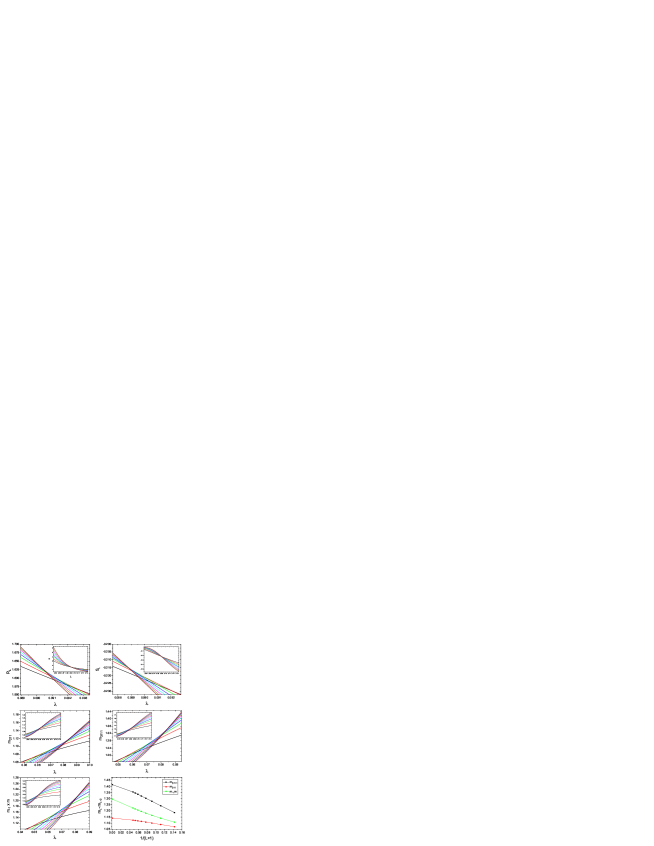
Figure 1: QS analysis: $R$, $S$, $m_{211}$, $m_{3111}$, $m_{-1}m$ in the neighborhood the crossings. The insets show these quantities over a larger range of $\lambda$ values. The lower-right panel shows the crossing values for $m_{211}$,$m_{-1}m_{1}$ and $m_{3111}$ (lower to upper) along with the extrapolated ($L\to\infty$) values.

Figure 2: Crossing values $\tilde{\beta}(L)$ versus $1/L$. The inset is a similar plot of the crossing points $\lambda_{S,L}$. The leftmost points are the extrapolated values using BST; curves are splines to the data and the BST extrapolations, intended as a guide to the eye. Error bars are smaller than the symbols.

In BST extrapolation bst the limiting value $T_{\infty}$ of a sequence $T_{j}$ ($j=1,2,3,...$), is estimated on the basis of the first $N$ terms via the recurrence relations

$$T_{m}^{(n)}=T_{m-1}^{(n+1)}+(T_{m-1}^{(n+1)}-T_{m-1}^{(n)})\left[\left(\frac{h_{n}}{h_{n+m}}\right)^{\omega}\left(1-\frac{T_{m-1}^{(n+1)}-T_{m-1}^{(n)}}{T_{m-1}^{(n+1)}-T_{m-2}^{(n+1)}}\right)-1\right]^{-1}$$ (5)

where, for $j=1,...,N$, $T_{-1}^{(j)}\equiv 0$, $T_{0}^{(j)}\equiv T_{j}$, and $h_{j}$ is a sequence converging to zero as $j\rightarrow\infty$. (Here $h_{j}=1/\bar{L}_{j}$, where $\bar{L}_{j}$ is the system size, or, for crossings, the mean value of the two system sizes involved.)

The BST procedure includes a free parameter, $\omega$, which can be adjusted to improve convergence. We use a convergence criterion similar to one employed in analyses of series expansions via Padé approximants privman ; rdiwanjsp , in which, varying some parameter, one seeks concordance amongst the estimates furnished by various approximants. In the present case, given $N$ values $T_{j}$, each associated with inverse system size $h_{j}$, we calculate $N+1$ estimates, one using the full set, and $N$ others obtained by removing one point, $(h_{k},T_{k})$, from the set. We search for values of $\omega$ that minimize the differences between the various estimates. Sweeping the interval $[0,5]$, we find that each quantity studied ($\tilde{\beta}$, $z$, moment ratios, and the associated estimates for $\lambda_{c}$) exhibits one or more crossings at which all $N+1$ estimates are equal to within numerical precision. Figure 3, for $\lambda_{c,S}$ (the estimate for $\lambda_{c}$ derived from the crossing values $\lambda_{S,L}$), illustrates the typical behavior. In this case there are four crossings, which fall at $\omega$ = 1.051380, 1.658703, 2.109962, and 2.550852; the associated values of $\lambda_{c,S}$ are 0.0904577, 0.0903878, 0.0902354, and 0.0900773.

To choose among the values when there are multiple crossings, we note that $\omega$ in the BST procedure is effectively a correction to scaling exponent. An independent estimate for this exponent can be obtained via a least-squares fit to the data using a double power-law form, for example,

$$\lambda_{S,L}=\lambda_{c,S}+\frac{A}{L^{y_{1}}}+\frac{B}{L^{y_{2}}}$$ (6)

with $y_{2}>y_{1}$. (The best-fit parameters $A$, $B$, $y_{1}$ and $y_{2}$ are determined by minimizing the variance of the differences $\delta_{L}\equiv\lambda_{S,L}-AL^{-y_{1}}-BL^{-y_{2}}$.) This yields $y_{1}=2.02$, leading us to take the average of the two values associated with the BST crossings nearest $y_{1}$, resulting in $\lambda_{c,S}=0.09016$. A similar procedure is used to obtain the other estimates listed in Tables 1 and 2. (We note that the apparent correction to scaling exponent $y_{1}$ falls in the range 2.02-2.23 for the crossing values of $\lambda$, and in the range 1.1-1.6 for the associated quantities $\tilde{\beta}$, z, and the moment ratios.)

Tables 1 and 2 include polynomial extrapolations as alternative estimates for the quantities of interest. (In this case we fit the data to a polynomial in $1/L$, using the highest possible degree. Polynomials of degree one or two smaller than maximum yield very similar results.) We adopt the mean of the BST and polynomial extrapolations as our best estimate, and adopt the difference between the two results as a rough estimate of the associated uncertainty. The situation is particularly favorable for determining $\lambda_{c}$ since we have five independent estimates. The average of the BST results is $\lambda_{c}=0.08996(7)$ while that from the polynomial fits is 0.09007(10), leading to our best estimate of $\lambda_{c}=0.09002(10)$. (Figures in parentheses denote uncertainties, given as one standard deviation.) The estimates for $\lambda_{c}$ and the moment ratios are consistent with simulation results, whereas those for $\beta/\nu_{\perp}$ and $z$ are not. (A detailed comparison is given in the following section.) Figure 4 shows the finite-size data and BST extrapolations for the various crossing values, $\lambda_{.,L}$.

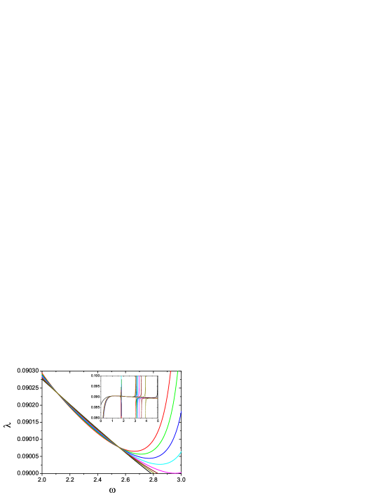
Figure 3: BST estimates (see text) for $\lambda_{c,S}$ versus extrapolation parameter $\omega$. Main graph: detail of interval [2,3]; inset: the full interval of study.

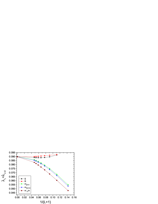
Figure 4: Crossing values $\lambda_{.,L}$ for $R_{L}$, $S_{L}$, $m_{211}$, $m_{3111}$ and $m_{-1}m_{1}$ (upper to lower).

The values for the kurtosis at $\lambda_{c}$ approach a limit of $q_{c}=-0.454(2)$ (see Fig. 5). For a given system size, $q(\lambda,L)$ exhibits a minimum in the vicinity of $\lambda_{c}$, as also observed in the contact process exact sol . Extrapolating $q(\lambda,L)$ to $L\to\infty$ for a series of values near $\lambda_{c}$, we obtain a function that exhibits a minimum near $\lambda=0.0947$ (the minimum value is -0.521). This implies that the minimum falls near, but not at the critical point, a conclusion supported by the simulation data reported in the following section. Turning to the scaled order-parameter variance $\chi$, we observe pronounced maxima even in small systems, as illustrated in Fig. 6. Estimates for $\tilde{\gamma}$ obtained from a local-slopes analysis of $\chi$ at the critical point $\lambda_{c}$ are listed in Table 2. (The local slope is defined so: $\tilde{\gamma}(L)\equiv\ln[\chi(L+1)/\chi(L-1)]/\ln[(L+1)/(L-1)]$.)

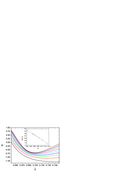
Figure 5: Kurtosis $q$ vs $\lambda$ for sizes $6$, $8$, …, $22$ (lower to upper). Inset: values for $q(L)$ at the critical point and our estimate for $q_{\lambda_{c},\infty}$.

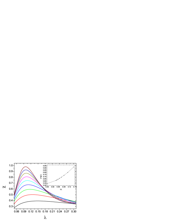
Figure 6: Scaled order parameter variance $\chi$ versus $\lambda$ for sizes $6$, $8$, …, $22$ (lower to upper). Inset: Estimates for $\gamma/\nu_{\perp}$ obtained via local-slopes analysis, and the extrapolated (infinite-size) value.

Table 1: Estimates for the critical sleeping rate $\lambda_{c}$ obtained via analysis of the QS probability distribution using BST extrapolation and polynomial fits.

Quantity	BST	Polynomial
$\lambda_{c,S}$	0.09016	0.09039
$\lambda_{c,R}$	0.08973	0.08993
$\lambda_{c,211}$	0.08999	0.09008
$\lambda_{c,3111}$	0.08995	0.09016
$\lambda_{c,-11}$	0.08998	0.08979

Table 2: Estimates for critical properties obtained via analysis of the QS probability distribution using BST extrapolation and polynomial fits.

Quantity	BST	Polynomial	Best Est.
$\beta/\nu_{\perp}$	0.2418	0.2405	0.241(1)
$z$	1.668	1.660	1.664(4)
$\gamma/\nu_{\perp}$	0.5428(1)	0.53942(1)	0.541(2)
$m_{211}$	1.1412	1.1422	1.1417(5)
$m_{3111}$	1.4151	1.4249	1.420(5)
$m_{-1}m$	1.2965	1.3203	1.308(12)
$q$	-0.460(5)	-0.454(4)	-0.457(6)

To estimate $\nu_{\perp}$, we determine $r^{\prime}\equiv|dm_{211,L}/d\lambda|_{\lambda_{c}}$ by constructing linear fits to the data on the interval $0.08992\leq\lambda\leq 0.09012$, using an increment of $\Delta\lambda=10^{-5}$. Since the graph of $\ln r^{\prime}$ versus $\ln L$ shows significant curvature, we analyze the local slopes, $\nu_{\perp}(L)=\ln[(L-1)/(L+1)]/\ln(r^{\prime}_{L-1}/r^{\prime}_{L+1})$. BST extrapolation of the latter yields $\nu_{\perp}=1.293(5)$. We obtain independent estimates for $\nu_{\perp}$ using the order parameter and flux of probability to the absorbing state, $r_{a}$, as described above, yielding 1.285(10) and 1.2644(2), respectively. On the basis of these results, we estimate $\nu_{\perp}=1.28(1)$.

IV Monte Carlo Simulations

IV.1 Simulation methods

We perform extensive simulations of the SRW model using both conventional and quasistationary (QS) methods. Quasistationary simulations howtosimulate ; quasidistr have proven to be an efficient method for studying absorbing state phase transitions, allowing one to obtain results of a given precision with an order of magnitude less CPU time than in conventional simulations. The method samples the QS distribution defined in the preceding section using a list of configurations saved during the evolution; when a visit to the absorbing state is imminent, the system is instead placed in a configuration chosen at random from the list. A detailed explanation of the method is given in howtosimulate .

We perform QS simulations using system sizes $L=100$, $200$, $400$,…, $32000$. Each realization of the process runs for $T=10^{9}$ time units, with the first $T_{R}=10^{8}$ time units discarded to ensure all transients have been eliminated. (Our time unit is defined below.) We use $1000$ saved configurations; the replacement probability (i.e., for replacing one of the configurations on the list with the current one) is $p_{rep}=10^{-5}.$ Our choice of $p_{rep}$ is guided by the condition $T>\tau_{M}>\tau$, where $\tau_{M}=M/p_{rep}$ is the mean time that a configuration remains on the list and $\tau$ is the mean lifetime in the QS state. The latter is estimated as $\tau=(T-T_{R})/N_{abs}$, where $N_{abs}$ is the number of (attempted) visits to the absorbing state for $t>T_{R}$. During the initial relaxation period ($t<T_{R}$) we use $p_{rep}=10^{-2}$ to eliminate the memory of the initial configuration. For each value of $\lambda$ studied, we calculate the mean and statistical uncertainties (given as one standard deviation) over $N_{R}=20$ independent realizations; for $L=16000$ we use $N_{R}=40$.

At each step of the simulation we select the particle involved from a list of active particles. The time increment associated with each step is $\Delta t=1/N_{a}$, where $N_{a}$ is the number of active particles just prior to the event. For $t>T_{R}$, we accumulate a histogram $h(N_{a})$ of the time during which there are exactly $N_{a}$ active particles. The normalized histogram is our best estimate for the probability distribution $P(N_{a})$, from which we may determine any desired moment of the order parameter $\rho=N_{a}/N$. The QS lifetime $\tau$ may also be obtained from $P(N_{a})$ via the relation $\tau_{h}=1/[\lambda P(1)]$, where the subscript $h$ serves only to distinguish this from the value $\tau$ found using the mean time between visits to the absorbing state.

IV.2 Scaling at the critical point

To determine $\lambda_{c}$, we first locate the crossings of the moment ratios $m_{211}$ (defined in Sec. III), for pairs of consecutive system sizes, and obtain a preliminary estimate by extrapolating the crossing values to $L\to\infty$. We then study larger systems using $\lambda$ values close to our preliminary estimate. Using these results, we determine the critical value via the familiar finite-size scaling criteria $\rho\sim L^{-\beta/\nu_{\perp}}$ and $\tau\sim L^{z}$, and the condition that $m_{211}$ approach a finite limiting value as $L$ increases. In logarithmic plots, $\rho$ and $\tau$ exhibit upward (downward) curvature for $\lambda<\lambda_{c}$ ($>\lambda_{c}$) as illustrated in Figs. 7 and 8; off-critical values are also readily identified in plots of $m_{211}$ versus $1/L$. Using these criteria we obtain $\lambda_{c}=0.090085(12)$. Of note are the strong finite-size corrections (evident in the insets of Figs. 7 and 8), for $L<1000$. Indeed, our estimates for critical exponents and moment ratios are obtained using only the data for $L\geq 1000$.

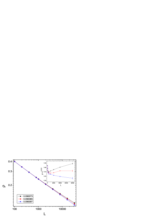
Figure 7: Order parameter $\rho$ versus system size $L$. Inset: $L^{0.212}\rho$ versus $L$. Lines are a guide to the eye.

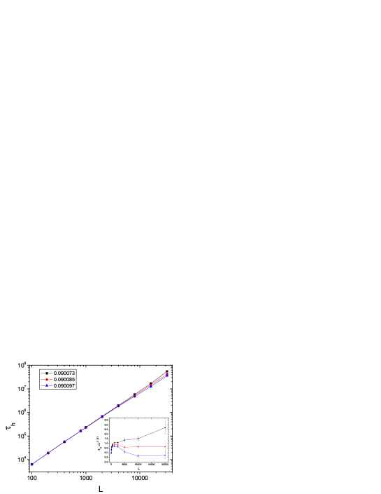
Figure 8: Lifetime $\tau_{h}$ versus system size $L$. Inset: $L^{-1.51}\tau_{h}$ versus $L$. Lines are a guide to the eye.

We turn now to FSS estimates of critical exponents. Using the data for $L\geq 1000$ we obtain $\beta/\nu_{\perp}=0.212(6)$ from analysis of $\rho$, and 0.217(10) from analysis of $m_{-1}$, which as noted in Sec. III, is expected to follow $m_{-1}(L,\lambda_{c})\propto L^{\beta/\nu_{\perp}}$. Analysis of the QS lifetime using $\tau$ and $\tau_{h}$ yields $z=1.50(4)$ and $z=1.51(4)$ respectively, while the data for the moment ratio yield $m_{211,c}=1.141(8)$. Restricting the analysis to the data for $L\geq 2000$, or for $L\geq 4000$, yields estimates for $\beta/\nu_{\perp}$, $m_{211,c}$, and $z$ consistent with the values cited above, but with somewhat larger uncertainties. Analysis of $\chi$ yields $\gamma/\nu_{\perp}=0.58(1)$. In all cases the chief contribution to the uncertainty is due to the uncertainty in $\lambda_{c}$ itself.

To estimate the exponent $\nu_{\perp}$ directly, we apply the method used in Sec. III, calculating the derivatives $r^{\prime}$ of quantities such as $\ln\rho$ and $\ln\tau$ with respect to $\lambda$ near the critical point. Using simulation data for $\lambda=0.090073$, $0.090085$, and $0.090097$, we construct a linear fit to estimate $r^{\prime}$ at $\lambda_{c}$. In Fig 9 we plot the values for $r^{\prime}$ obtained via analysis of $|d\ln\rho/d\lambda|$, $dm_{211}/d\lambda$ and $|d\ln\tau/d\lambda|$. The estimates obtained using the data for $L\geq 1000$ are listed in Table 3; based on these results we estimate $\nu_{\perp}=1.31(4)$. Since the values obtained using different quantities are quite different, this exponent is not determined to good precision.

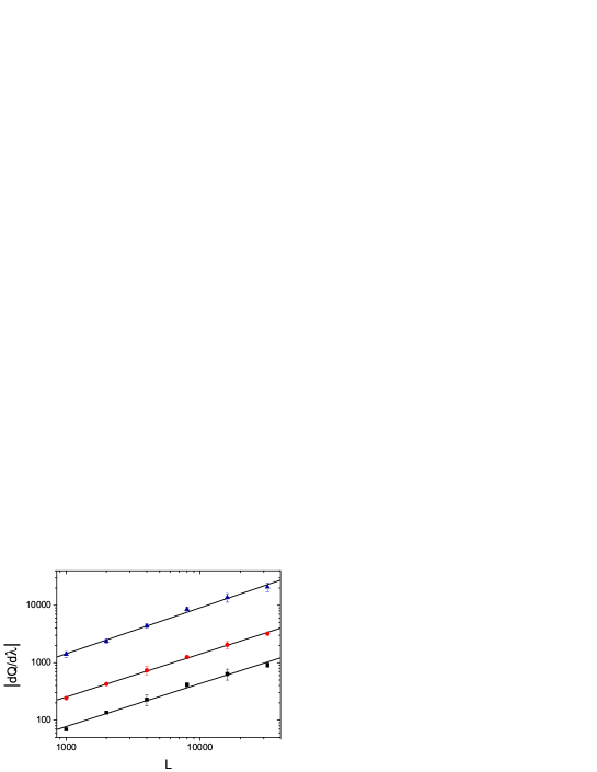
Figure 9: Derivatives $r^{\prime}\equiv|dQ/d\lambda|_{\lambda_{c}}$ for $m_{211}$ (squares), $\ln\rho$ (circles) and $\ln\tau$ (triangle). Lines are linear fits to the data, with slopes of $0.746(37)$, $0.749(16)$, and $0.80(3)$ (lower to upper).

Table 3: Estimates for $\nu_{\perp}$ obtained from the derivatives of $m_{211}$, $\ln\rho$ and $\ln\tau$.

$r^{\prime}\equiv|dQ/d\lambda|_{\lambda_{c}}$	$Q\equiv m_{211}$	$Q\equiv\ln(\rho)$	$Q\equiv\ln(\tau)$
$1000\leq L\leq 32000$	$1.34(7)$	$1.34(4)$	$1.25(5)$

Next we examine the QS probability distribution $P_{L}(\rho,\lambda)$ for the fraction of active particles, $\rho=N_{a}/N$. At the critical point, this distribution is expected to take the scaling form densprob ,

$$P_{L}(\rho,\lambda_{c})=\frac{2}{\langle\rho\rangle L}\tilde{P}(\rho/\langle\rho\rangle),$$ (7)

where $\tilde{P}$ is a normalized scaling function. (The prefactor arises from normalization of $P_{L}$, with $N=L/2$.) Figure 10 is a scaling plot of the QS probability distribution at the critical point, showing evidence of a data collapse, albeit with significant finite-size corrections (the maximal scatter of the values is about 2%); the collapse is quite good for the two largest system sizes. Also shown are scaled probability distributions for the one-dimensional conserved restricted stochastic sandpile sandpile2006 , showing good overall agreement.

Figure 11 shows the behavior of the order-parameter moment ratios $m_{211}$, $m_{3111}$, the reduced fourth cumulant $q$, and $m_{-1}m$, defined in Sec. III. Our estimates for the critical values are given in Table 5).

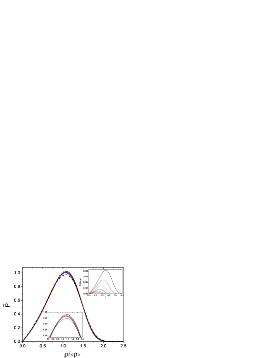
Figure 10: Main figure: scaling function ${\tilde{P}}\equiv(\langle\rho\rangle L/2)P_{L}(\rho/\langle\rho\rangle)$ versus $\rho/\langle\rho\rangle$ for system sizes $L=1000$, $2000$,…,$L=32\,000$ (lower to upper). The dotted and dashed curves show the corresponding result for the one-dimensional restricted stochastic sandpile, for $L=20\,000$ and $50\,000$, respectively. Lower inset: detail of the region in which $\tilde{P}$ takes its maximum. Upper inset: unscaled data (system sizes increasing from upper to lower).

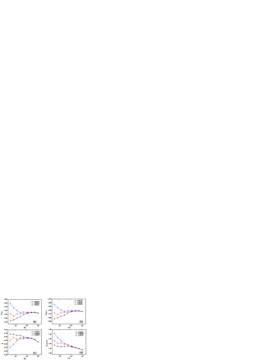
Figure 11: Moment ratios (a) $m_{211}$; (b) $m_{3111}$; (c) reduced fourth cumulant $q$; and (d) $m_{-1}m$ versus system size $L$.

IV.3 Off-critical scaling behavior

It is of interest to study the scaling of the order parameter, of the scaled variance and of the lifetime, away from the critical point. Although off-critical scaling properties have been amply verified for models in the directed percolation universality class, such as the contact process densprob ; livrodickman , finite-size scaling and associated data collapse of the order parameter is more problematic in one-dimensional stochastic sandpile models sandpile2002 ; sandpile2006 .

FSS analysis implies that the order parameter take the form $\rho(\Delta,L)\sim L^{-\beta/\nu_{\perp}}f(\Delta L^{1/\nu_{\perp}})$, where the scaling function is $f(x)\propto x^{\beta}$ for $x\gg 1$. In the inactive phase, $\lambda>\lambda_{c}$, the number of active particles in the QS regime is ${\cal O}(1)$, so that $\rho\propto L^{-1}$, leading to $f(x)\sim|x|^{\beta-\nu_{\perp}}$. Alternatively, writing $\rho(\Delta,L)\sim\Delta^{\beta}h(\Delta L^{1/\nu_{\perp}})$, the scaling function must satisfy $h(x)\propto x^{-\beta}$ for $x\rightarrow 0$, while in the inactive phase $h(x)\propto|x|^{-\nu_{\perp}}$. FSS analysis predicts that the scaled variance take the form $\chi(L,\Delta)\sim L^{\gamma/\nu_{\perp}}g(\Delta L^{1/\nu_{\perp}})$, with $g(x)\propto x^{-\gamma}$ for $x\gg 1$ and $g(x)\propto|x|^{-(\nu_{\perp}+\gamma)}$ in the inactive phase.

Figure 12 shows a good data collapse of the order parameter in the forms $\rho^{*}\equiv L^{\beta/\nu_{\perp}}\rho$ and $\tilde{\rho}\equiv\rho\Delta^{-\beta}$, and of the scaled order-parameter variance $\chi^{*}\equiv\chi L^{-\gamma/\nu_{\perp}}$, as functions of $\Delta^{*}\equiv\Delta L^{1/\nu_{\perp}}$, using data for system sizes from $L=100$ to $32000$. The exponents associated with the best collapses are listed in Table 4. Based on these results, we estimate $\beta/\nu_{\perp}=0.216(4)$, $\beta=0.29(1)$ and $\gamma/\nu_{\perp}=0.57(1)$. We note that the values found for $\nu_{\perp}$ in the active and inactive regimes differ slightly, leading to best estimate $\nu_{\perp}=1.30(4)$.

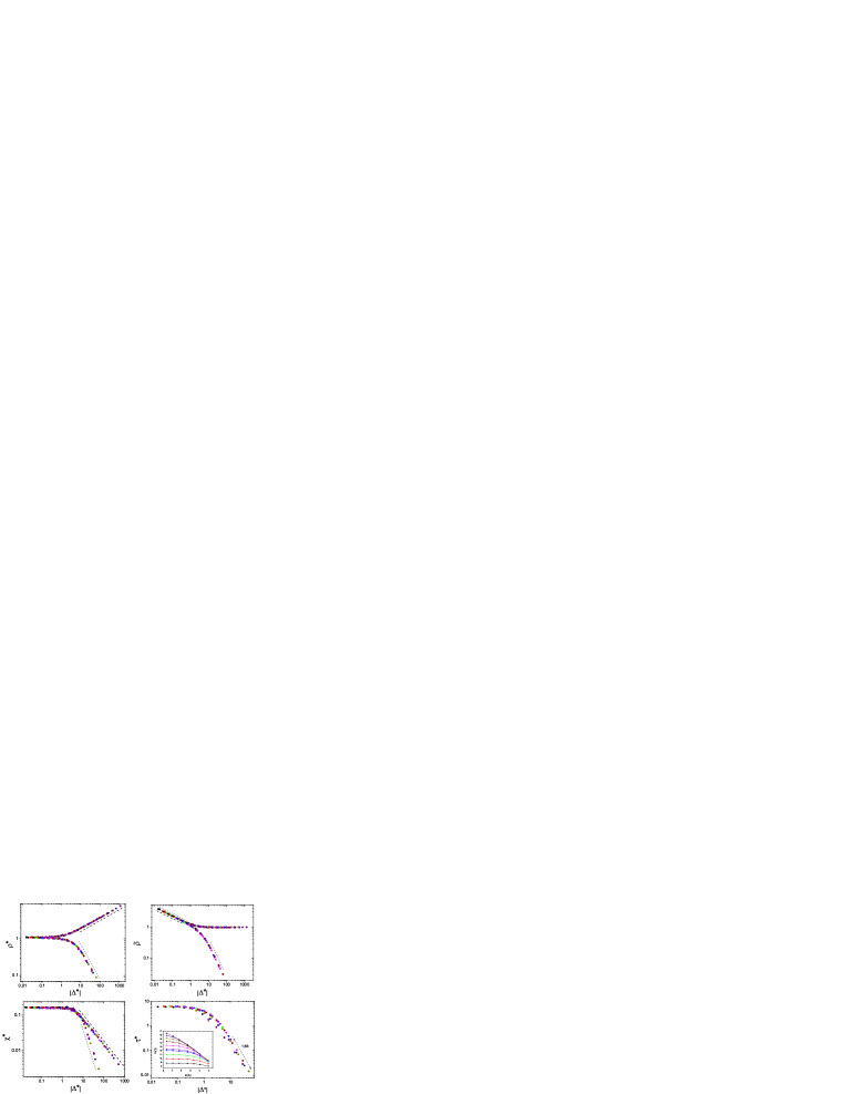
Figure 12: Scaled order parameter $\rho^{*}\equiv\rho L^{\beta/\nu_{\perp}}$ (upper left) and $\tilde{\rho}\equiv\rho\Delta^{-\beta}$ (upper right), scaled variance $\chi^{*}\equiv\chi L^{-\gamma/\nu_{\perp}}$ (lower left) and the scaled lifetime $\tau^{*}\equiv L^{-z}\tau$ (lower right) versus scaled distance from critical point, $\Delta^{*}\equiv\Delta L^{1/\nu_{\perp}}$, in the active and inactive phases (upper and lower set of points, respectively). The best-fit exponents associated with the data collapses are given in Table 4. The slopes of the dashed and dotted lines represent the power laws exhibited by the scaling functions in the active and inactive phase, respectively.

In the active phase, $\lambda<\lambda_{c}$, a data collapse of $\rho^{*}$ versus $\Delta^{*}$ is obtained over about four orders of magnitude in $\Delta^{*}$. Interestingly, such a data collapse is only observed over a much smaller interval - about one order of magnitude - in stochastic sandpiles for a comparable range of lattice sizes sandpile2006 ; sandpile2009 . A linear fit to the data (using all sizes) for $\Delta^{*}>10$ yields $\beta=0.293(2)$. Using $\tilde{\rho}$ versus $\Delta^{*}$ we found $\beta=0.288(3)$, including the data for $\Delta^{*}<0.2$. The data for $\chi^{*}$ (for $\Delta^{*}>10$) yield $\gamma=0.733(7)$. The power laws associated with these exponents are represented in Figure 12 by dashed lines. Using the hyperscaling relation $\gamma=d\nu_{\perp}-2\beta$, the latter results and the exponents used in the collapses in the active phase, one finds (a) $\beta=(1.32(3)-0.733(7))/2=0.29(2)$; (b) $\beta/\nu_{\perp}=(1-\gamma/\nu_{\perp})/2=(1-0.568)/2=0.216(5)$; and (c) $\nu_{\perp}=\gamma+2\beta=0.733(7)+0.580(8)=1.31(2)$. These predictions are consistent with the values used in the collapses and with those obtained at the critical point.

Table 4: Critical exponent estimates from off-critical simulations. For each scaling relation (first column), we list the associated exponent obtained via a fit to the data (second column). The third and fourth columns give the exponents obtained via data collapse. $x$ denotes the argument of the relevant scaling function.

Active phase
$\rho^{*}\propto x^{\beta}$	$\beta$ = 0.293(2)	$\beta/\nu_{\perp}$ = 0.218(5)	$\nu_{\perp}$ = 1.34(3)
$\tilde{\rho}\propto x^{-\beta}$	$\beta$ = 0.288(3)	$\beta$ = 0.293(3)	$\nu_{\perp}$ = 1.32(3)
$\chi^{*}\propto x^{-\gamma}$	$\gamma$ = 0.733(7)	$\gamma/\nu_{\perp}$ = 0.568(8)	$\nu_{\perp}$ = 1.32(3)
Inactive phase
$\rho^{*}\sim x^{\beta-\nu_{\perp}}$	$\beta-\nu_{\perp}=-0.95(4)$	$\beta/\nu_{\perp}$ = 0.214(2)	$\nu_{\perp}$ = 1.26(2)
$\tilde{\rho}\sim x^{-\beta}$	$\beta=0.29(1)$	$\nu_{\perp}=1.22(5)$	$\nu_{\perp}$ = 1.26(3)
$\chi^{*}\sim x^{-(\nu_{\perp}+\gamma)}$	$\nu_{\perp}+\gamma=1.85(4)$	$\gamma/\nu_{\perp}$ = 0.57(1)	$\nu_{\perp}$ = 1.28(3)
$\tau^{*}\sim x^{-\nu_{\parallel}}$	$\nu_{\parallel}=1.86(6)$	$\nu_{\parallel}/\nu_{\perp}$ = 1.53(3)	$\nu_{\perp}$ = 1.30(2)

Similarly, the scaled quantities $\rho^{*},\,\tilde{\rho}$ and $\chi^{*}$ exhibit a good collapse in the inactive phase, for all system sizes studied, as shown in Fig. 12. Using $\rho^{*}$, a linear fit to the data for $|\Delta^{*}|>20$ yields $\nu_{\perp}-\beta=-0.95(4)$. Using the result from the best collapse we have $\beta=0.95(4)-1.26(2)=0.29(4)$. Analyzing the data collapse for $\tilde{\rho}$ we find $\beta=0.29(1)$ in the small-$|\Delta^{*}|$ regime. In the opposite limit we obtain $\nu_{\perp}=1.22(5)$ as illustrated in the dotted lines in Fig. 12. Finally, the data collapse of $\chi^{*}$ versus $\Delta^{*}$ leads to $\nu_{\perp}+\gamma=1.85(4)$. Combining these results, the hyperscaling relation used above, and the values from the best collapses shown in Table 4 for $\chi^{*}$, one can predict: (a) $\gamma/\nu_{\perp}=0.57(1)\,\Rightarrow\,\gamma=0.57(1)\times 1.28(3)=0.73(3)$, (b) $\beta/\nu_{\perp}=(1-\gamma/\nu_{\perp})/2=(1-0.57(1))/2=0.215(5)$ and (c) $\gamma=1.85(4)-1.28(3)=0.57(5)$. The first two relations are consistent with the exponent values obtained previously, while the third conflicts with the value for $\gamma$ found for $\lambda\leq\lambda_{c}$. This may reflect a violation of scaling, but the possibility that our study does not probe sufficiently deep into the inactive regime, for which one expects $\chi\sim 1/L$, cannot be discarded.

In the inactive phase, the lifetime $\tau$ is expected to follow $\tau(\Delta,L)=|\Delta|^{-\nu_{\parallel}}G(\Delta L^{1/\nu_{\perp}})$, with the scaling function $G(x)\propto|x|^{-\nu_{\parallel}}$, implying a data collapse if we plot $\tau^{*}=L^{-z}\tau$ versus $\Delta^{*}$. As shown in Fig. 12, the collapse here is much poorer than in the other cases. A linear fit to the data for $L\leq 8000$ and $\Delta^{*}>10$ furnishes $\nu_{\parallel}=1.86(6)$. This result is in concordance with the scaling relation $z=\nu_{\parallel}/\nu_{\perp}$, if we employ the values found at the critical point ($z=1.50(4)$ and $\nu_{\perp}=1.34(6)$) and the best-collapse values ($z=1.53(3)$ and $\nu_{\perp}=1.30(2)$); the latter yield the value $\nu_{\parallel}=1.53(3)\times 1.30(2)=1.99(8)$, consistent (to within uncertainty) with the value found via collapse.

IV.4 Approach to the quasistationary regime

Yet another aspect of scaling at an absorbing-state phase transition involves the approach to the QS regime, starting from a maximally active initial condition. The quantities of interest are the time-dependent activity density $\rho(t)$ and the moment ratio $m_{211}(t)$. At short times (i.e., before the QS regime is attained), at the critical point, the expected scaling behavior for the order parameter is $\rho\sim t^{-\delta}f(t/\tau)$ where the scaling function $f(x)\sim x^{\delta}$, for $x\gg 1$, with $\delta=\beta/\nu_{\parallel}$. One expects $m_{211}-1\sim t^{1/z}$ for $t\ll\tau$.

To probe this regime we perform conventional simulations for the same system sizes as used in QS simulations; averages are calculated over $N_{R}=1000$ independent realizations; each runs until the system reaches the absorbing state or attains a maximum time, $t_{max}=10^{8}$. We use the critical point value $\lambda_{c}=0.090085$ found in QS simulations. We determine $\rho(t)$ and $m_{211}(t)$ as averages over surviving realizations on time intervals that for large $t$ represent uniform increments of $\ln(t)$, a procedure known as logarithmic binning.

The evolution of $\rho$ as a function of $t$ is shown in Fig. 13. Unlike the contact process, in which $\rho$ follows a simple power law before attaining the QS regime, in the SRW model the relaxation is more complicated. Absence of simple power-law relaxation of the activity density has also been noted for stochastic sandpiles cssp1d . We calculate the local slope $\delta(t)$ via piece-wise linear fits to the data for $\ln\rho$ versus $\ln t$ on the interval $[t/\alpha,\alpha t]$, with $\alpha=1.76$ (that is, about 30 data points, with an increment of 0.1 in $\ln t$). The inset of Fig. 13 shows $\delta(t)$ decreasing systematically with time, from around $0.145$ to approximately $0.12$ over the interval studied. (Note that the data for longer times come from larger systems.) If we associate with the short- and long-time regimes the values $\delta_{short}\approx 0.143(3)$ and $\delta_{long}\approx 0.121(3)$, then the scaling relation $\delta=\beta/\nu_{\parallel}=\beta/(\nu_{\perp}z)$ yields $\delta=0.212/1.50=0.14$, in good agreement with the short-time value. Plotting $\rho^{*}=L^{\beta/\nu_{\perp}}\rho$ as a function of $t^{*}=t/L^{z}$ we observe a good collapse of the data for different system sizes in the first regime using $z=1.50$, and in the second regime if we use $z=1.72$. In both cases the best collapse is obtained using $\beta/\nu_{\perp}=0.215$.

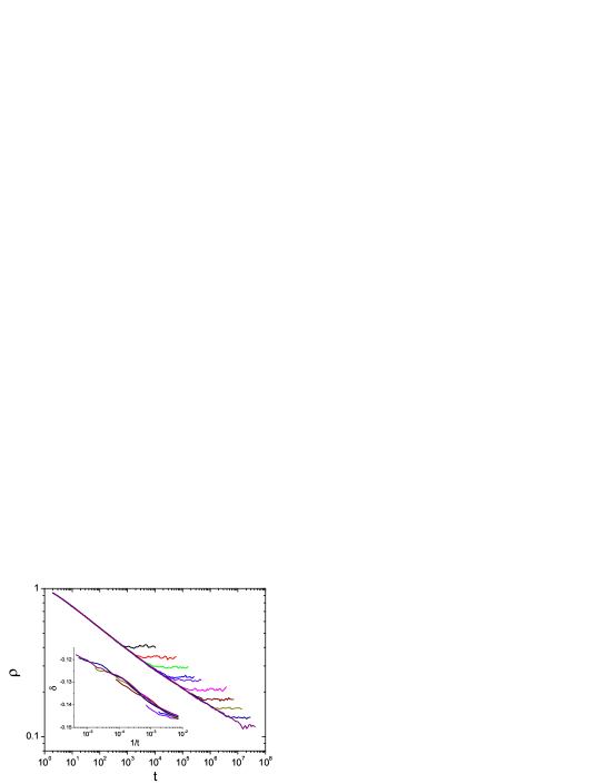
Figure 13: Active particle density $\rho$ versus $t$. System sizes $L=100$, $200$, $400$,…,$L=32000$ (from upper to lower). The inset shows the local slope of $\rho(t)$ versus $1/t$.

In contrast to the complicated behavior of the activity density, the quantity $m_{211}(t)-1$ exhibits simple power-law scaling over four or more decades. Using $t^{*}=t/L^{z}$ with $z=1.71$, we obtain a good data collapse for all system sizes studied, as shown in Fig. 14. The relation $m_{211}-1\sim t^{1/z}$ yields $z=1.70(1)$, consistent with the collapse values for $m_{211}$ and $\rho(t)$ in the long-time regime, but clearly inconsistent with $z=1.50(4)$ found using FSS analysis in the QS regime. Curiously, $m_{211}$ shows no hint of the crossover exhibited by the order parameter. Note that the value $\delta=0.121(2)$ associated with the second regime of the order parameter is consistent with $\beta/\nu_{\perp}=0.212$ and $z=1.71$. Thus the scaling of $m_{211}$ follows, from the beginning, that observed in $\rho$ in the long-time regime.

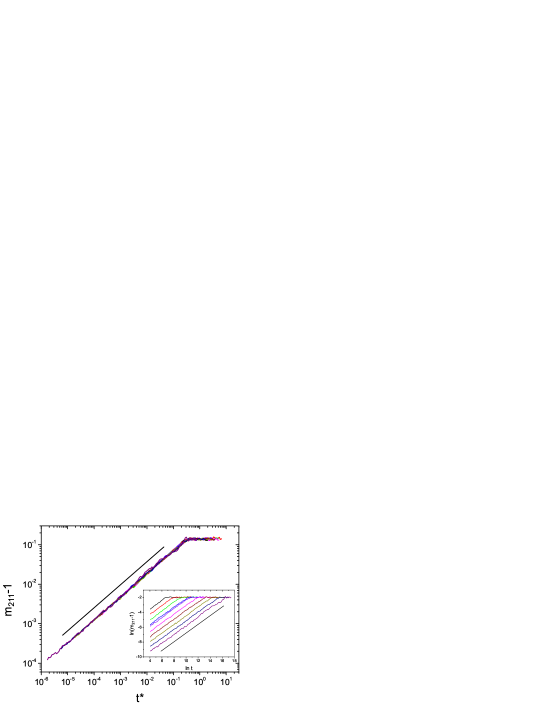
Figure 14: Scaling plot of $m_{211}-1$ versus $t^{*}=t/L^{z}$ at the critical point, using $z=1.70$, for system sizes up to $32\,000$. The inset shows the unscaled data for $100\leq L\leq 32000$ (from top to bottom). The slope of the straight lines is $0.587$.

IV.5 Comparison of exact QS and simulation results

In Table 5 we compare results obtained via exact analysis of small systems (QSA) and simulation. The results are consistent to within uncertainty except for the dynamic exponent $z$. The QSA predictions for $\beta/\nu_{\perp}$ and (especially) $z$ seem less reliable than those derived from simulation. On the other hand, the QSA estimates for moment rations are nominally of higher precision than the simulation results. Care must be exercised, however, since the QSA analysis may be subject to relatively large finite-size corrections. (The present study and previous works on models in the CDP class suggest that corrections to scaling and finite-size effects are stronger for this class than for the contact process.) Table 5 also includes results on sandpiles and the conserved lattice gas. The agreement between these studies and the present work is quite good, leaving little doubt that the SRW model belongs to the same universality class as stochastic conserved sandpiles and conserved directed percolation.

Table 5: Comparison of critical properties of the SRW model found via exact analysis of small systems (QSA) and Monte Carlo simulation (MC), and results from previous studies (Prev) on models in the CDP class: $a$: restricted stochastic sandpile sandpile2006 ; $b$: conserved lattice gas kockelkoren ; $c$: restricted stochastic sandpile unpub .

Quantity	QSA	MC	Prev
$\lambda_{c}$	0.09002(10)	0.090085(12)
$\beta/\nu_{\perp}$	0.241(1)	0.212(6)	0.213(6) a
$\beta$		0.290(4)	0.289(12)a
$\gamma/\nu_{\perp}$	0.541(2)	0.58(1)	0.55(1) c
$\nu_{\perp}$	1.28(1)	1.33(5)	1.36(2) a
$z$	1.664(4)	1.50(4)	1.55(3) b
$m_{211}$	1.142(1)	1.141(8)	1.142(8) a
$m_{3111}$	1.420(5)	1.415(26)	1.425(25)c
$m_{-1}m$	1.308(12)	1.327(27)	1.332(10)c
$q_{c}$	-0.454(2)	$-0.47(3)$	-0.46(3) c

V Discussion

We study sleepy random walkers (SRW) in one dimension using (numerically) exact quasistationary analysis of small systems and Monte Carlo simulation. Based on considerations of symmetry and conserved quantities, one expects the SRW process to belong to the conserved directed percolation (CDP) class, typified by conserved stochastic sandpiles. Our results for critical exponents and moment ratios support this conclusion. Different from most examples of the CDP class studied until now, the SRW process includes a continuously-variable control parameter which facilitates simulation and numerical analysis.

The present work represents a further test of the exact QS analysis proposed in exact sol . In addition to locating the critical point with good precision, QS analysis furnishes fair results for the critical exponent $\nu_{\perp}$ and quite good estimates for the moment ratios $m_{211}$ and $m_{3111}$. While somewhat better than the preliminary study of a model in the CDP class, QSA predictions for the SRW model are not of the quality obtained for the contact process exact sol . This appears to be connected with the stronger finite-size effects and corrections to scaling observed for models in the CDP class. Exact analysis of QS properties is nevertheless a useful complement to simulation, as in this method the long-time behavior (conditioned on survival) is surely attained, whereas simulations are subject to the nagging possibility of insufficient relaxation time. The QS calculations typically require (for the largest system studied) several days on a reasonably fast computer, that is, a small fraction of the time invested in a simulation study.

In Monte Carlo simulations, we test various scaling relations via data collapse, in both the sub- and supercritical regimes, and compare the resulting critical exponents with those obtained via finite-size scaling at the critical point. The results are generally consistent between the regimes, as well as with those of previous studies of stochastic conserved sandpiles. Despite the general agreement, we identify several inconsistencies and examples of anomalous behavior. First, the estimates for the exponent $\nu_{\perp}$ in the inactive phase are significantly smaller (by roughly 5%) than those obtained at the critical point or in the active phase. Second, and more significantly, the relaxation of the order parameter to its quasistationary value at the critical point is marked by two apparent scaling regimes, with associated exponents $z_{short}=1.50$, $\delta_{short}=0.143$, $z_{long}=1.71$, and $\delta_{long}=0.121$, respectively. Paradoxically, $z_{short}$ is close to the dynamic exponent characterizing finite-size scaling in the asymptotic long-time (i.e., quasistationary) regime. A similar two-regime relaxation is observed in the one-dimensional conserved stochastic sandpile cssp1d ; the latter study reports $z_{long}=1.75(3)$ and somewhat larger values for the exponents $\delta$. Despite these minor numerical differences it seems likely that anomalous relaxation is a characteristic of the CDP class in general. Finally, we have noted a possible violation of scaling associated with the scaled variance of the order parameter $\chi$ in the inactive phase.

Given the complex pattern of relaxation of the order parameter, it is surprising that $m_{211}-1$, another quantity expected to exhibit power-law scaling at the critical point, in fact shows a near-perfect data collapse in a single scaling regime that corresponds essentially to the two scaling regimes of the order parameter. The associated dynamic exponent is $z=1.71(1)$, the same as $z_{long}$ to within uncertainty. This exponent is however considerably larger than the dynamic exponent $z=1.50(4)$ associated with finite-size scaling at the critical point. As discussed in scaling , the difference may reflect the existence of two time scales, one associated with the relaxation of the order parameter to its QS value, the other related to the finite-size lifetime. These two times scale in the same manner at absorbing phase transitions in models without a conserved density, such as the CP. These unexpected findings should motivate further study of the SRW and related models, with the goal of a complete and coherent picture of scaling in the CDP universality class. From the present vantage it appears that such a picture will be significantly more complex than for directed percolation.

Acknowledgment

We are grateful to CNPq, Brazil, for financial support.

References

- (1) H. Hinrichsen, Adv. Phys. 49, 815 (2000).
- (2) J. Marro and R. Dickman, Nonequilibrium Phase Transitions in Lattice Models (Cambridge University Press, Cambridge, 1999).
- (3) S. Lübeck, Int. J. Mod. Phys. B 18, 3977 (2004).
- (4) G. Ódor, Rev. Mod. Phys. 76, 663 (2004).
- (5) K. A. Takeuchi, M. Kuroda, H. Chaté, and M. Sano, Phys. Rev. Lett. 99, 234503, 2007.
- (6) A. L. Lin et al., Biophys. J. 87, 75 (2004).
- (7) L. Corté, P.M. Chaikin, J. P. Gollub and D. J. Pine, Nat. Phys. 4 420 (2008).
- (8) T. E. Harris, Ann. Probab. 2, 969 (1974).
- (9) A. Vespignani, S. Zapperi and V. Loreto, J. Stat. Phys, 88, 47 (1997).
- (10) S. S. Manna, J. Phys. A 24, L363 (1991).
- (11) S. S. Manna, J. Stat. Phys. 59, 509 (1990).
- (12) R. Dickman and R. Vidigal, Braz. J. Phys. 33, 73 (2003)
- (13) R. Dickman. Phys. Rev. E 77, 030102(R) (2008).
- (14) R. Dickman, L. T. Rolla, and V. Sidoravicius, J Stat. Phys. 138, 126 (2010).
- (15) R. Dickman. Phys. Rev. E 65, 047701 (2002).
- (16) M. E. Fisher and M. N. Barber, Phys. Rev. Lett. 28, 1516 (1972).
- (17) Finite-size Scaling and Numerical Simulations of Statistical Systems, edited by V. Privman (World Scientific, Singapore, 1990).
- (18) J. R. G. de Mendonça, J. Phys. A 32, L467 (1999).
- (19) R. Dickman and J. Kamphorst Leal da Silva, Phys. Rev. E 58, 4266(R) (1998).
- (20) K. Binder, Phys. Rev. Lett. 47, 693 (1981); Z. Phys. B 43, 119 (1981).
- (21) M. M. de Oliveira and R. Dickman, Phys. Rev. 71, 016129 (2005).
- (22) R. Dickman and R. Vidigal, J. Phys. A 35, 1147 (2002).
- (23) W. Press, S. Teukolsky, W. Vetterling, and B. Flannery, Numerical Recipes (Cambridge University Press, Cambridge, 1992).
- (24) M. Henkel and G. Schütz, J. Phys. A 21, 2617 (1988).
- (25) V. Privman, J. Phys. A 16, 3097 (1983).
- (26) I. Jensen and R. Dickman, J. Stat. Phys. 71, 89 (1993).
- (27) T. Aukrust, D. A. Browne and I. Webman, Phys. Rev. A 41, 5294 (1990).
- (28) R. Dickman, T. Tomé, and M. J. de Oliveira, Phys. Rev. E 66, 016111 (2002).
- (29) R. Dickman, Phys. Rev. E 73, 036131 (2006).
- (30) S. D. da Cunha, R. R. Vidigal, L. R. da Silva, and R. Dickman, Eur. Phys. J. B 72, 441 (2009).
- (31) R. da Silva, R. Dickman, and J. R. Drugowich de Felcio, Phys. Rev. E 70, 067701 (2004).
- (32) S. B. Lee and S.-G. Lee, Phys. Rev. E 78, 040103R (2008) (and references therein.)
- (33) J. Kockelkoren and H. Chaté, e-print cond-mat/0306039.
- (34) R. Dickman, unpublished.
- (35) R. Dickman, M. Alava, M. A. Muñoz, J. Peltola, A. Vespignani, and S. Zapperi, Phys. Rev. E 64, 056104 (2001).