Breaking parameter degeneracy in interacting dark energy models from observations

Abstract

We study the interacting dark energy model with time varying dark energy equation of state. We examine the stability in the perturbation formalism and the degeneracy among the coupling between dark sectors, the time-dependent dark energy equation of state and dark matter abundance in the cosmic microwave background radiation. Further we discuss the possible ways to break such degeneracy by doing global fitting using the latest observational data and we get a tight constraint on the interaction between dark sectors.

I Introduction

It is convincing that cold dark matter (DM) and dark energy (DE) are two dominant sources governing the evolution of our universe. Considering that these two components are independent is a very specific assumption, in the framework of field theory it is more natural to consider the inevitable interaction between them secondref . An appropriate interaction in the dark sectors can alleviate the coincidence problem and understand why energy densities of dark sectors are of the same order of magnitude today 10 -14 .

However, it was suspected that the coupling between dark sectors might lead to the curvature perturbation instability x . This problem was later clarified in y where it was shown that the stability of curvature perturbation holds by appropriately choosing the forms of the interaction and the values of the constant equation of state (EOS) of the DE. Another possibility to cure the instability was suggested in z .

The observational signature of the interaction between dark sectors has been widely discussed 10 -AbdallaPLB09 . It was found that the coupling in dark sectors can affect significantly the expansion history of the universe and the growth history of cosmological structures. A number of studies have been devoted to grasp the signature of the dark sectors mutual interaction from the probes of the cosmic expansion history by using the WMAP, SNIa, BAO and SDSS data etc 71 -pp . Interestingly it was disclosed that the late ISW effect has the unique ability to provide insight into the coupling between dark sectors hePRD09 . Furthermore, complementary probes of the coupling within dark sectors have been carried out in the study of the growth of cosmic structure 31 -AbdallaPLB09 . It was found that a non-zero interaction between dark sectors leaves a clear change in the growth index 31 ; Caldera ; peacock . In addition, it was argued that the dynamical equilibrium of collapsed structures such as clusters would acquire a modification due to the coupling between DE and DM pt ; AbdallaPLB09 , which could leave the signature in the virial masses of clusters AbdallaPLB09 . The imprint of dark sectors interaction in the cluster number counts was disclosed in bb . N-body simulations of structure formation in the context of interacting DE models were studied in Baldi .

Since both DE and DM are currently only detected via their gravitational effects and any change in the DE density is conventionally attributed to its equation of state $w$, there is an inevitable degeneracy while extracting the signature of the interaction between dark sectors and other cosmological parameters. The degeneracies among the dark sector coupling, the the equation of state (EoS) of DE and the DM abundance were first discussed in he2010 . In the formalism of the perturbation theory, it was found that the degeneracy can be broken and tighter constraint on the interaction between dark sectors can be obtained from observations.

In he2010 , the EoS of DE was taken to be constant. Recently, more accurate data analysis tells us that the time varying DE gives a better fit than a cosmological constant Yin9 . The time varying EoS influences a lot on the universe evolution, perturbation stability and it must affect the constraint on the interaction between dark sectors. Thus it is of great interest to generalize the discussion in he2010 to the interacting DE model with time-dependent DE EoS. The observational constraints on an interacting DE with time varying EoS were discussed in 75 ; beans . In this work we will first discuss the stability of the perturbation and the degeneracy between the dark sector interaction and the time varying EoS of DE. Furthermore we will explore possible ways to break the degeneracy among the dark sectors’ coupling, the time-dependent DE EoS and the DM abundance. In our study we will use the popular Chevallier-Polarski-Linder (CPL) parametrization Gong9 to describe the time varying DE EoS, which expresses the EoS in terms of the scale factor in the form $w(a)=aw_{0}+(1-a)w_{e}$. In the early time, $a\ll 1$, $w\simeq w_{e}$. At the present time when $a\simeq 1$, $w\simeq w_{0}$.

II perturbation formalism and its stability

In the spatially flat Friedmann-Robertson- Walker(FRW) background, if there is an interaction between DE and DM, neither of them can evolve independently. The (non)conservation equations are described by

$$\rho_{c}^{\prime}+3\mathcal{H}\rho_{c}=aQ_{c},$$ (1)

$$\rho_{d}^{\prime}+3\mathcal{H}(1+w)\rho_{d}=aQ_{d},$$ (2)

where the subscript c represents DM and d stands for DE. $Q_{\lambda}$ is the term leading to energy transfer. Considering that there is only energy transfer between DE and DM, we have $Q_{c}=-Q_{d}=Q$. The sign of $Q$ determines the direction of the energy transfer. For positive $Q$, the energy flows from DE to DM. For negative $Q$, the energy flow is reversed. In our following study, we adopt the phenomenological interaction in the form $Q=3\xi H\rho_{c}$, where $\xi$ is the coupling constant. This merely repeats the analysis of [10], where the energy transfer was assumed to be proportional to the energy density, but here we have the energy density times the Hubble parameter. In [7], it was indicated that qualitatively similar conclusions apply to both cases. The presence of DM energy density in the interaction was shown problematic in the stability of perturbation x . It was argued that only for constant EoS of DE in the phantom region, this interaction form can be viable and effective to alleviate the coincidence problemy . It is of interest to explore this interaction form when the DE EoS is time-dependent with the CPL parametrization, especially when the DE EoS is in the quintessence region.

As discussed in he2010 , the coupling vector is specified in co-moving frame as

$$Q^{\nu}_{(\lambda)}=(\frac{Q_{(\lambda)}}{a},0,0,0)^{T}.$$

The perturbed form of the zero component $\delta Q^{0}_{(\lambda)}$ can be uniquely determined from the background energy-momentum transfer and has the form

$$\delta Q^{0}_{(\lambda)}=-\Psi Q_{(\lambda)}/a+\delta Q_{(\lambda)}/a.$$

While the spatial component of the perturbed energy-momentum transfer $\delta Q^{i}_{(\lambda)}$ can be set to zero since there is no non-gravitational interaction in the DE and DM coupled system and only the inertial drag effect appears in the system due to the stationary energy transfer between DE and DM as discussed in he2010 .

The perturbation equations for DM and DE have the forms he2010 ; 31

$$D_{c}^{\prime} =-kU_{c}+3\mathcal{H}\xi\Psi-3\xi\Phi^{\prime}\quad,$$

$$U_{c}^{\prime} =-\mathcal{H}U_{c}+k\Psi-3\mathcal{H}\xi U_{c}\quad;$$

$$D_{d}^{\prime} =-3\mathcal{H}(C^{2}_{e}-w)D_{d}-9\mathcal{H}^{2}(C^{2}_{e}-C^{2}_{a})\frac{U_{d}}{k}$$

$$+\{3w^{\prime}-9\mathcal{H}(w-C^{2}_{e})(\xi r+1+w)\}\Phi$$

$$+3\xi r\Phi^{\prime}-3\mathcal{H}\xi r\Psi+3\mathcal{H}\xi r(D_{d}-D_{c})$$

$$-9\mathcal{H}^{2}(C^{2}_{e}-C^{2}_{a})\xi r\frac{U_{d}}{(1+w)k}-kU_{d}\quad,$$

$$U_{d}^{\prime} =-\mathcal{H}(1-3w)U_{d}-3C^{2}_{e}(\xi r+1+w)k\Phi$$

$$+3\mathcal{H}(C^{2}_{e}-C^{2}_{a})\xi r\frac{U_{d}}{1+w}+3\mathcal{H}(C^{2}_{e}-C^{2}_{a})U_{d}$$

$$+kC^{2}_{e}D_{d}+(1+w)k\Psi+3\mathcal{H}\xi rU_{d}.$$

$r=\rho_{c}/\rho_{d}$ is the ratio of DM to DE. In the above, $C^{2}_{a}=w<0$. However, it is not clear what expression we should have for $C^{2}_{e}$ . In x it has been argued in favor of $C^{2}_{e}=1$. This is correct for the scalar field, but it is not obvious for other cases. The most dangerous possibility, as far as instabilities are concerned, is $C^{2}_{e}=1\neq C^{2}_{a}=w<0$ since the first term in the second line of the equation of $U_{d}$ can lead to the blow up when $w$ is close to $-1$. Assuming that $C^{2}_{e}=1,C^{2}_{a}=w$, the last two equations above for DE can be rewritten as

$$D_{d}^{\prime} =3\mathcal{H}(-1+w+\xi r)D_{d}-9\mathcal{H}^{2}(1-w)(1+\frac{\xi r}{1+w})\frac{U_{d}}{k}$$

$$-kU_{d}+\{3w^{\prime}+9\mathcal{H}(1-w)(\xi r+1+w)\}\Phi+3\xi r\Phi^{\prime}$$

$$-3\mathcal{H}\xi r\Psi-3\mathcal{H}\xi rD_{m}\quad,$$

$$U_{d}^{\prime} =-2\mathcal{H}(1+\frac{3\xi r}{1+w})U_{d}+kD_{d}-3(\xi r+1+w)k\Phi$$

$$+(1+w)k\Psi.$$

Numerically, we find that the first two terms on the RHS of the perturbation equations for DE contribute more than other terms to the divergence. In order to explain the reason for the blow-up, we keep the leading terms and use $\xi r\sim-w$ in the early universe y . In the early universe $w\sim w_{e}$ and the above equations can be reduced in the form

$$D_{d}^{\prime} =-3\mathcal{H}D_{d}-9\mathcal{H}^{2}\frac{1-w_{e}}{1+w_{e}}\frac{U_{d}}{k}\quad,$$

$$U_{d}^{\prime} =2\mathcal{H}\frac{1-2w_{e}}{1+w_{e}}U_{d}+kD_{d}.$$

The second order differential equation for $D_{d}$ can be written as

$$D^{\prime\prime}_{d}=\bigg{(}2\frac{\mathcal{H}^{\prime}}{\mathcal{H}}-\frac{1+7w_{e}}{1+w_{e}}\mathcal{H}\bigg{)}D^{\prime}_{d}+3(\mathcal{H}^{\prime}-\mathcal{H}^{2})D_{d}.$$

In the radiation dominated period, we have $\mathcal{H}\sim 1/\tau,\mathcal{H}^{\prime}\sim-1/\tau^{2}$, thus

$$D^{\prime\prime}_{d}=-3\frac{1+3w_{e}}{1+w_{e}}\frac{D^{\prime}_{d}}{\tau}-\frac{6}{\tau^{2}}D_{d},$$

which gives the solution

$$D_{d}=C_{1}\tau^{r_{+}}+C_{2}\tau^{r_{-}},$$

where

$$r_{\pm}=-\frac{1+4w_{e}+\pm\sqrt{-5-4w_{e}+10w_{e}^{2}}}{1+w_{e}}.$$

When $r_{\pm}$ is a real positive value, the perturbation will blow up. In y for the constant DE EoS, $w$ was required to be smaller than $-1$ to accommodate the stability. For the DE EoS with CPL parametrization, in the early time $w\simeq w_{e}<-1$ can also allow negative $r_{\pm}$ to provide stability. Moreover as shown in Fig.1 when $w\simeq w_{e}>-1/4$ in the early time, the stability can be safely protected as well.

Figure 1: The Behavior of the indices $r_{\pm}$. $r_{+}$ and $r_{-}$ meet at the point where the square root becomes zero. The real part of $r_{\pm}$ are the same on the right side of this point.

When $-1<w_{e}<-1/4$, the above approximate analytical analysis cannot help, we need to count on the numerical calculation to see the stability of perturbation in the early universe. Results are shown in Fig.2. When $w_{e}$ falls in this range, the perturbation grows slower for weaker coupling. When the existing dark sector coupling is weak enough, it has the possibility to keep the perturbation stable. For smaller $w_{e}$ in the range $-1<w_{e}<-1/4$, weaker interaction is required to keep the stability in perturbation.

(a)

(b)

Figure 2: The evolution of the curvature perturbation and DE density perturbation for various $\xi$ when $-1<w_{e}<-1/4$.

Thus unlike the constant DE with $w>-1$, the time varying DE can allow stable perturbation when it is interacting with DM. However in some ranges of $w$ in the quintessence region, in order to keep the stability in the perturbation we have the upper limit on the strength of the interaction. When the DE EoS is in the phantom region, the stability of the perturbation is always protected in the presence of the interaction between dark sectors, which is the same as the case we observed for the constant EoS of DE y .

III degeneracies of interaction, DE EoS and DM abundance in CMB spectrum

With the perturbation formalism at hand, we can study the influence of the interaction between dark sectors and other cosmological parameters on the CMB power spectrum. We will concentrate our attention on the DE EoS in the quintessence region $w>-1$, since it has different property as discussed in the above section compared with the case with constant EoS. In Fig.3 we illustrate the theoretical computation results of the CMB power spectrum for changing $w_{0},w_{e}$ in the CPL parametrization of DE EoS and coupling constant $\xi$ but with DM abundance fixed.

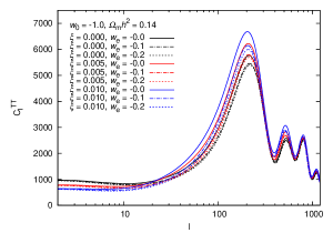
(a) $w_{e}\sim\xi$

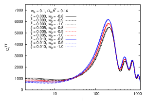
(b) $w_{0}\sim\xi$

Figure 3: The dependences of CMB angular power spectrum on the time varying DE EoS and the coupling between dark sectors.

We see in the CMB TT angular power spectrum that the change of the $w_{e}$ only modifies the acoustic peaks, while it does not influence the low-l part of the spectrum. The influence of $w_{0}$ is on the contrary, it changes little of the acoustic peaks, but influences more on the small-l spectrum. When $w_{0}$ decreases, low-l spectrum will be suppressed. Different effects given by $w_{e}$ and $w_{0}$ on CMB spectrum are interesting. Since we have more CMB data in large-l than small-l spectrum, it is easier to constrain $w_{e}$ than $w_{0}$. This can be used to explain the fitting results in the following.

The above discussion is for the fixed coupling constant. If we allow the change of $\xi$, we see that at the acoustic peaks, $\xi$ plays more important role in the change of the spectrum than the influence of $w_{e}$. In the low-l region, we also observe that $\xi$ effect is more important than $w_{0}$ to suppress the CMB spectrum.

The above discussion is valid for fixed DM abundance. Now we investigate the dependence of CMB angular power spectrum on the abundance of matter, $\omega_{m}=\Omega_{m}h^{2}$. Since the abundance of baryon is fixed, it is identical to investigate the effect of the abundance of CDM. Although the abundance of the DM does not affect much on the low-l CMB power spectrum, it quite influences the amplitude of the first and second acoustic peaks in CMB TT angular power spectrum (see Fig.4). Decreasing $\omega_{m}$ will enhance the acoustic peaks. This effect is degenerated with the influence given by the dark sectors’ interaction and $w_{e}$ as we observed in Fig.3. A possible way to break this degeneracy is to consider the influence of the interaction on the low-l CMB spectrum. Moreover, we can include further observations to get a complementary constraint on the matter abundance and this in turn can help to constrain the coupling between dark sectors.

Figure 4: The dependence of CMB angular power spectrum on the DM abundance.

In order to extract the signature of the interaction and put constraints on other cosmological parameters, we need to use the latest CMB data together with other observational data. We report the results of fitting in the next section.

IV fitting results

In this section we confront our models with observational data by implementing joint likelihood analysis. We take the parameter space as

$$P=(h,\omega_{b},\omega_{m},\tau,\ln[10^{10}A_{s}],n_{s},\xi,w_{0},w_{e})$$

where $h$ is the hubble constant, $\omega_{b}=\Omega_{b}h^{2},\omega_{m}=\Omega_{m}h^{2}$, $A_{s}$ is the amplitude of the primordial curvature perturbation, $n_{s}$ is the scalar spectral index, $\xi$ is the coupling constant when we choose the interaction in proportion to the energy density of DM. To avoid the negative energy density of DE in the early time of the universeheJCAP08 , we limit the coupling constant $\xi$ to be positive which indicates the energy flow from DE to DM. $w_{0},w_{e}$ are parameters in the CPL parametrization of DE EoS. Since we concentrate on the DE EoS in the quintessence region, we set the limit $-1<w_{0}<0,-1<w_{e}<0$ in our data fitting. We choose the flat universe with $\Omega_{k}=0$ and our work is based on CMBEASY codeeasy . The fitting results are listed in Table.1.

When we only use the CMB anisotropy data from the seven-year Wilkinson Microwave Anisotropy Probe (WMAP), in Fig.5 we show the 1d marginalized likelihoods for all of the primary MCMC parameters of our model. It is clear that, just from CMB data, the constraint on $w_{0}$ is worse than that on $w_{e}$. This is consistent with the analysis we did in the theoretical study. The $w_{e}$ affects more on the acoustic peaks. More observational CMB data there can help to constrain $w_{e}$ well. For our model with the interaction between dark sectors in proportion to the energy density of DM, we find that CMB data alone can impose tight constraints on couplings and $\Omega_{m}h^{2}$. This can be understood by using our theoretical analysis that the degeneracy between the coupling and the DM abundance can be broken by looking at the low-l CMB spectrum.

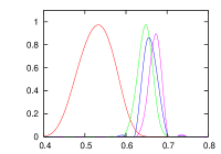
(a) $h$

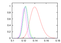
(b) $\Omega_{m}h^{2}$

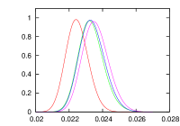
(c) $\Omega_{b}h^{2}$

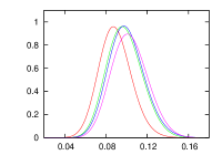
(d) $\tau$

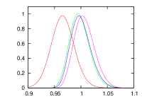
(e) $n$

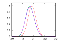
(f) ${\rm ln}10^{10}A_{s}$

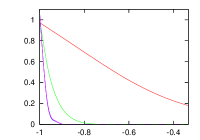
(g) $w_{0}$

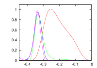
(h) $w_{e}$

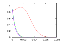
(i) $\xi$

(j)

Figure 5: 1-D marginalized likelihoods for cosmological parameters. WMAP alone (red), WMAP+BAO(green), WMAP+SN(blue) and WMAP+BAO+SN(purple)

Table 1: The cosmological parameters from the global fitting.

Parameter	WMAP	WMAP+BAO	WMAP+SN	WMAP+BAO+SN
$\Omega_{m}h^{2}$	$0.140^{+0.009}_{-0.008}$	$0.124^{+0.004}_{-0.004}$	$0.123^{+0.004}_{-0.004}$	$0.121^{+0.004}_{-0.004}$
$\Omega_{b}h^{2}$	$0.0224^{+0.0007}_{-0.0006}$	$0.0232^{+0.0008}_{-0.0007}$	$0.0233^{+0.0008}_{-0.0007}$	$0.0235^{+0.0008}_{-0.0007}$
$h$	$0.532^{+0.041}_{-0.046}$	$0.647^{+0.018}_{-0.018}$	$0.659^{+0.015}_{-0.015}$	$0.669^{+0.013}_{-0.013}$
$\tau$	$0.087^{+0.016}_{-0.015}$	$0.096^{+0.012}_{-0.016}$	$0.098^{+0.018}_{-0.016}$	$0.101^{+0.018}_{-0.017}$
$n$	$0.965^{+0.022}_{-0.021}$	$0.994^{+0.020}_{-0.017}$	$0.996^{+0.020}_{-0.017}$	$1.003^{+0.021}_{-0.018}$
${\rm ln}[10^{10}A_{s}]$	$3.083^{+0.037}_{-0.036}$	$3.064^{+0.039}_{-0.037}$	$3.064^{+0.040}_{-0.038}$	$3.065^{+0.041}_{-0.039}$
$w_{0}$	$<-0.629(68\%{\rm C.L.})$	$<-0.943(68\%{\rm C.L.})$	$<-0.978(68\%{\rm C.L.})$	$<-0.977(68\%{\rm C.L.})$
$w_{e}$	$-0.25^{+0.09}_{-0.05}$	$-0.33^{+0.03}_{-0.02}$	$-0.33^{+0.02}_{-0.02}$	$-0.34^{+0.02}_{-0.02}$
$\xi$	$<0.0026(68\%{\rm C.L.})$	$<0.0006(68\%{\rm C.L.})$	$<0.0005(68\%{\rm C.L.})$	$<0.0005(68\%{\rm C.L.})$

In order to get tighter constraint on $\Omega_{m}h^{2}$, we use the BAO distance measurements BAO which are obtained from analyzing clusters of galaxies and test a different region in the sky as compared to CMB. BAO measurements provide a robust constraint on the distance ratio

$$d_{z}=r_{s}(z_{d})/D_{v}(z)$$ (3)

where $D_{v}(z)\equiv[(1+z)^{2}D_{A}^{2}z/H(z)]^{1/3}$is the effective distance Eisenstein , $D_{A}$ is the angular diameter distance, and $H(z)$ is the Hubble parameter. $r_{s}(z_{d})$ is the comoving sound horizon at the baryon drag epoch where the baryons decoupled from photons. We numerically find $z_{d}$ using the condition $\int_{\tau_{d}}^{\tau_{0}}\dot{\tau}/R=1,R=\frac{3}{4}\frac{\rho_{b}}{\rho_{\gamma}}$ as defined in wayne . The $\chi^{2}_{BAO}$ is calculated as BAO ,

$$\chi^{2}_{BAO}=(\vec{\textbf{d}}-\vec{\textbf{d}}^{obs})^{T}\textbf{C}^{-1}(\vec{\textbf{d}}-\vec{\textbf{d}}^{obs})$$ (4)

where $\vec{\textbf{d}}=(d_{z=0.2},d_{z=0.35})^{T}$, $\vec{\textbf{d}}^{obs}=(0.1905,0.1097)^{T}$ and the inverse of covariance matrix read BAO

$$\textbf{C}^{-1}=\left(\begin{array}[]{cc}30124&-17227\\ -17227&86977\\ \end{array}\right).$$ (5)

Furthermore, we add the BAO A parameter BAO_A ,

$$A = \frac{\sqrt{\Omega_{m}}}{E(0.35)^{1/3}}\left[\frac{1}{0.35}\int_{0}^{0.35}\frac{dz}{E(z)}\right]^{2/3}$$ (6)

$$= 0.469(n_{s}/0.98)^{-0.35}\pm 0.017$$

where $E(z)=\frac{H(z)}{H_{0}}$ and $n_{s}$ are the scalar spectral index. In order to improve the constraints on the DE EoS $w$, we use the compilation of 397 Constitution samples from supernovae survey SNeIa . We compute

$$\chi^{2}_{SN}=\sum\frac{[\mu(z_{i})-\mu_{obs}(z_{i})]^{2}}{\sigma_{i}^{2}}\quad,$$ (7)

and marginalize the nuisance parameter.

We implement the joint likelihood analysis,

$$\chi^{2}=\chi^{2}_{WMAP}+\chi^{2}_{SN}+\chi^{2}_{BAO}.$$ (8)

The cosmological parameters are well constrained. When the coupling between dark sectors is proportional to the energy density of DM, its constraint is much tighter than that from CMB data alone. The likelihoods of the fitting results for the matter abundance, parameters $w_{0},w_{e}$ for DE EoS are also improved. Compared with the WMAP data alone, we see that the joint analysis by including other observational data provides tighter constraints on the cosmological parameters.

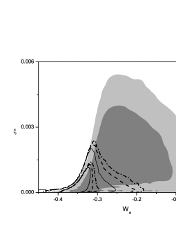
Figure 6: The 2-D marginalized confidence contours for $\xi$ and $w_{e}$. WMAP alone(in shades), WMAP+BAO(dash-dotted lines), WMAP+SNIa (dashed lines) and WMAP+BAO+SN data (solid lines).

In Fig.6 we plot the 2d marginalized likelihood for the interacting models from our MCMC run with CMB and other observational data. The shaded regions are the result from WMAP alone at $68\%$ and $95\%$ C.L. If we just look at the CMB result, we see that when $w_{e}<-1/4$, the allowed $\xi$ becomes smaller when $w_{e}$ decreases. When $w_{e}>-1/4$, the allowed $\xi$ is bigger. This fitting result supports our theoretical observation obtained in the stability analysis. The dashed and solid lines are the $68\%$ and $95\%$ C. L. regions in combination of WMAP+SNIa and WMAP+BAO+SN data sets, respectively. Fig.6 summarizes our findings for the possible relation between $w_{e}$ and the coupling constant from data fitting.

V conclusions and discussions

In this paper we generalized our previous studyhe2010 on the interacting DE model to the DE with time varying EoS. We reviewed the perturbation theory and examined the stability in different model parameters. Based upon the perturbation formalism we have studied the signature of the interaction between dark sectors from CMB angular power spectrum. Theoretically we found that there are possible ways to break the degeneracies among the interaction, parameters in CPL parametrization of DE EoS and DM abundance. This can help to get tight constraint on the interaction between DE and DM.

We have performed the global fitting by using the CMB power spectrum data from WMAP7Y results together with the latest SNIa, and BAO data to constrain the interaction between DE and DM and other cosmological parameters. As anticipated from our theoretical analysis, the global fitting can really break degeneracy of cosmological parameters and give tighter constraints on the interaction between dark sectors, DE EoS and DM abundance. The relation between $w_{e}$ and the coupling obtained from the fitting supports the result got in the stability analysis.

With the successful experience to deal with the interacting DE model with time varying DE EoS, our next step is to extend our study to the field theory based model to describe the interaction between dark sectors. The preliminary attempt was carried out in secondref . More efforts are required on this direction.

- (1) Sandro Micheletti, Elcio Abdalla, Bin Wang, Phys. Rev. D79 (2009) 123506; Sandro M.R. Micheletti, JCAP 1005 (2010) 009.
- (2) L. Amendola, Phys. Rev. D 62, 043511 (2000); L. Amendola and C. Quercellini, Phys. Rev. D 68 (2003) 023514 ; L. Amendola, S. Tsujikawa and M. Sami, Phys. Lett. B 632 (2006) 155.
- (3) D. Pavon, W. Zimdahl, Phys. Lett. B 628 (2005) 206; S. Campo, R. Herrera, D. Pavon, Phys. Rev. D 78 (2008) 021302(R).
- (4) C. G. Boehmer, G. Caldera-Cabral, R. Lazkoz, R. Maartens, Phys. Rev. D 78 (2008) 023505.
- (5) G. Olivares, F. Atrio-Barandela and D. Pavon, Phys. Rev. D 74 (2006) 043521.
- (6) S. B. Chen, B. Wang, J. L. Jing, Phys.Rev. D 78 (2008) 123503.
- (7) J. Valiviita, E. Majerotto, and R. Maartens, JCAP 07, 020 (2008), ArXiv:0804.0232.
- (8) J. H. He, B. Wang, and E. Abdalla, Phys. Lett. B 671, 139 (2009), ArXiv:0807.3471.
- (9) P. Corasaniti, Phys. Rev. D 78, 083538 (2008); B. Jackson, A. Taylor, and A. Berera, Phys. Rev. D 79, 043526 (2009).
- (10) J. Valiviita, E. Majerotto, R. Maartens, JCAP 07 (2008) 020, ArXiv:0804.0232.
- (11) J. H. He, B. Wang, E. Abdalla, Phys. Lett. B 671 (2009) 139, ArXiv:0807.3471.
- (12) P. Corasaniti, Phys. Rev. D 78 (2008) 083538; B. Jackson, A. Taylor, A. Berera, Phys. Rev. D 79 (2009) 043526.
- (13) D. Pavon, B. Wang, Gen. Relav. Grav. 41 (2008) 1; B. Wang, C. Y. Lin, D. Pavon, E. Abdalla, Phys. Lett. B 662 (2008) 1.
- (14) B. Wang, J. Zang, C. Y. Lin, E. Abdalla and S. Micheletti, Nucl. Phys. B 778 (2007) 69.
- (15) F. Simpson, B. M. Jackson, J. A. Peacock, ArXiv:1004.1920v2.
- (16) W. Zimdahl, Int. J. Mod. Phys. D 14 (2005) 2319.
- (17) Z. K. Guo, N. Ohta and S. Tsujikawa, Phys. Rev. D 76 (2007) 023508.
- (18) C. Feng, B. Wang, E. Abdalla, R. K. Su, Phys. Lett. B 665 (2008) 111; X. M. Chen, Y. G. Gong, E. N. Saridakis, JCAP 0904:001,(2009).
- (19) J. Valiviita, R. Maartens, E. Majerotto, Mon. Not. Roy. Astron. Soc. 402 (2010) 2355-2368, ArXiv:0907.4987.
- (20) J. Q. Xia, Phys. Rev. D 80 (2009) 103514, ArXiv:0911.4820.
- (21) J. H. He, B. Wang, P. Zhang, Phys. Rev. D 80 (2009) 063530, ArXiv:0906.0677.
- (22) M. Martinelli, L. Honorez, A. Melchiorri, O. Mena Phys. Rev. D 81 (2010) 103534, arXiv:1004.2410; L. Honorez, B. Reid, O. Mena, L. Verde, R. Jimenez, JCAP 1009 (2010) 029, ArXiv:1006.0877.
- (23) J.H. He, B. Wang, JCAP 06 (2008) 010, ArXiv:0801.4233.
- (24) J. H. He, B. Wang, Y. P. Jing, JCAP 07 (2009) 030, ArXiv:0902.0660.
- (25) G. Caldera-Cabral, R. Maartens, B. Schaefer, JCAP 0907 (2009) 027.
- (26) F. Simpson, B. Jackson, J. A. Peacock, arXiv: 1004.1920.
- (27) J. H. He, B. Wang, E. Abdalla, D. Pavon, JCAP 1012:022, 2010, arXiv: 1001.0079.
- (28) O. Bertolami, F. Gil Pedro and M. Le Delliou, Phys. Lett. B 654 (2007) 165. O. Bertolami, F. Gil Pedro and M. Le Delliou, Gen. Rel. Grav. 41 (2009) 2839-2846, ArXiv:0705.3118.
- (29) E. Abdalla, L.Raul W. Abramo, L. Sodre Jr., B. Wang, Phys. Lett. B 673 (2009) 107; E. Abdalla, L. Abramo, J. Souza, Phys. Rev. D 82 (2010) 023508, ArXiv:0910.5236.
- (30) M. Baldi, arXiv:1005.2188.
- (31) J. H. He, B. Wang, E. Abdalla, arXiv:1012.3904, Phys. Rev. D (in press).
- (32) U. Alam, V. Sahni, and A. Starobinsky, JCAP 0406, 008 (2004); Y. G. Gong, Class. Quant. Grav. 22, 2121 (2005); Y. Wang and M. Tegmark, Phys. Rev. D 71, 103513 (2005); Y. Wang and P. Mukherjee, Astrophys. J. 606, 654 (2004); R. Daly and S. Djorgovski, Astrophys. J. 612, 652 (2004); U. Alam, V. Sahni, T. Saini, and A. Starobinsky, Mon. Not. Roy. Astron. Soc. 354, 275 (2004); T. Choudhury and T. Padmanabhan, Astron. Astrophys. 429, 807 (2005).
- (33) R. Bean, E. Flanagan, I. Laszlo, M. Trodden, Phys. Rev. D 78:123514, 2008.
- (34) M. Chevallier and D. Polarski, Int. J. Mod. Phys. D 10, (2001) 213; E. V. Linder, Phys. Rev. Lett. 90, 091301 (2003).
- (35) M. Doran, JCAP 10 (2005) 011.
- (36) W. J. Percival et al., Mon. Not. Roy. Astron. Soc. 401 (2010) 2148, ArXiv:0907.1660.
- (37) Eisenstein D. J., et al., Astrophys. J. 633 (2005) 560.
- (38) Hu W., Sugiyama N., Astrophys. J. 471 (1996) 542.
- (39) Eisenstein D. J. et al., Astrophys. J. 633 (2005) 560.
- (40) A. G. Riess, et al., Astrophys.J. 659 (2007) 98, ArXiv:astro-ph/0611572.
- (41) Riess, A. G. et al., Astrophys. J. 699 (2009) 539.