Fast transport of Bose-Einstein condensates

Abstract

We propose an inverse method to accelerate without final excitation the adiabatic transport of a Bose Einstein condensate. The method, applicable to arbitrary potential traps, is based on a partial extension of the Lewis-Riesenfeld invariants, and provides transport protocols that satisfy exactly the no-excitation conditions without constraints or approximations. This inverse method is complemented by optimizing the trap trajectory with respect to different physical criteria and by studying the effect of noise.

Introduction.—A major goal of atomic physics is the comprehensive control of the atomic quantum state for fundamental research and applications in interferometry, metrology, or information processing. The ability to manipulate Bose-Einstein condensates may be particularly rewarding due, for example, to their potential in interferometric sensors, but it is also challenging, as their low temperatures make them more fragile than ordinary cold atoms. A basic operation is the transport of the condensate to appropriate locations such as a “science chamber”, or to launch or stop the atomic cloud. This transport has been performed with several techniques based on adiabatic, slow motion to avoid excitations and losses Ketterle2002 ; H_Nature ; Denschlag06 ; Xiong . Long transport times, however, may be counterproductive since the condensate is more exposed to noise and decoherence, and also limit severely the repetition rates and signal to noise ratios. Fast, non-adiabatic but “faithful” transport of cold atoms, i.e., leading to the desired final state, has also been investigated experimentally David and theoretically Calarco ; Masuda ; transport . For the Schrödinger equation (SE) an inverse engineering method based on constructing Lewis-Riesenfeld invariants and corresponding dynamical modes (solutions of the SE formed by invariant eigenvectors times a phase factor) provides a “shortcut to adiabaticity” ChPRL1 ; Nice . However the invariant concept, i.e., an operator satisfying $dI/dt\equiv{\partial I(t)}/{\partial t}+[I(t),H(t)]/({i\hbar})=0$ with constant expectation values for arbitrary states that evolve with the Hamiltonian $H$, is not directly applicable to the non-linear Gross-Pitaevskii equation (GPE). In fact previous extensions of this inverse technique to expansions of condensates required special regimes or time-dependent Feshbach resonance control MCh ; Nice2 ; Adolfo . By contrast, we show in this letter that the transport of a condensate scales in the right way for applying a generalized inverse method, so that no approximations or limits are required to design fast processes without final excitation. Strictly speaking we do not construct invariants as in the linear theory but, as far as ground-state to ground-state transport is concerned, the formal structure of the dynamical transport modes of the linear case remains valid for the GPE. This will be illustrated with a numerical example and compared with a direct method. In the final part of the article we shall optimize the trap trajectory according to several criteria, since the invariant-based inverse engineering provides a family of possible transport solutions, an analyze the effect of noise.

General setting.—Our starting point is the GPE for potentials whose Schrödinger dynamics admit a quadratic invariant in momentum LL ; transport ; Lohe ,

$$i\hbar\frac{\partial\psi({\mathbf{q}},t)}{\partial t}=\bigg{[}-\frac{\hbar^{2}}{2m}\nabla^{2}_{{\mathbf{q}}}-{\bf F}(t)\cdot{\mathbf{q}}+\frac{1}{2}m\omega^{2}(t)|{\bf q}|^{2}$$

$$+\frac{1}{\rho^{2}}U\bigg{(}\frac{{\bf q}-\boldsymbol{\alpha}}{\rho}\bigg{)}+g_{{}_{D}}|\psi({\mathbf{q}},t)|^{2}+f(t)\bigg{]}\psi({\mathbf{q}},t),$$ (1)

where $f=f(t)$ is arbitrary, $\nabla^{2}_{\mathbf{q}}$ is the Laplacian in Cartesian coordinates for $D=1$, 2, or 3 dimensions, $U$ is an arbitrary potential function of the argument ${\boldsymbol{\sigma}}\equiv({\mathbf{q}}-\boldsymbol{\alpha})/\rho$ and $\omega(t)$, the force ${\mathbf{F}}(t)$, $\boldsymbol{\alpha}=\boldsymbol{\alpha}(t)$ and the scaling function $\rho=\rho(t)$ satisfy

$$\omega_{0}^{2}/\rho^{3} = \ddot{\rho}+\omega^{2}(t)\rho,$$ (2)

$${\mathbf{F}}(t)/m = \ddot{\boldsymbol{\alpha}}+\omega^{2}(t)\boldsymbol{\alpha},$$ (3)

where $\omega_{0}$ is a constant and the dots represent time derivatives. The physical meaning of $\boldsymbol{\alpha}$ depends on the process type, see transport , and will be clarified below. The wave function is normalized to one. Without the non-linear term, an arbitrary solution of Eq. (1) can be written as a linear combination of the eigenvectors $\psi_{n}$ of the dynamical invariant $I$ LR , $\psi(\mathbf{q},t)=\sum_{n}c_{n}e^{i\alpha_{n}(t)}\psi_{n}(\mathbf{q},t)$, $I(t)\psi_{n}(\mathbf{q},t)=\lambda_{n}\psi_{n}(\mathbf{q},t)$, where the amplitudes $c_{n}$ and the eigenvalues $\lambda_{n}$ are constants. Here $\psi_{n}$ is normalized to one, but continuum, delta-normalized states are also possible. The Lewis-Riesenfeld phases $\alpha_{n}$ satisfy $\hbar\,\frac{d\alpha_{n}}{dt}=\left\langle\psi_{n}\left|i\hbar\frac{\partial}{\partial t}-H\right|\psi_{n}\right\rangle$ LR ; DL . A single mode solution of the SE ($g_{{}_{D}}=0$) takes the form

$$e^{i\alpha_{n}}\psi_{n}({\mathbf{q}},t)=\rho^{-D/2}e^{\frac{im}{\hbar\rho}[\dot{\rho}|{\mathbf{q}}|^{2}/2+(\dot{\boldsymbol{\alpha}}\rho-\boldsymbol{\alpha}\dot{\rho})\cdot{\mathbf{q}}]}$$

$$\times e^{-\frac{i}{\hbar}\int_{0}^{t}\!\!dt^{\prime}\Big{\{}\frac{m\left[|\dot{\boldsymbol{\alpha}}\rho-\boldsymbol{\alpha}\dot{\rho}|^{2}-\omega_{0}^{2}|\boldsymbol{\alpha}|^{2}/\rho^{2}\right]}{2\rho^{2}}+f\Big{\}}}\phi_{n}(\boldsymbol{\sigma},\tau),$$ (4)

where we have introduced a scaled time $\tau=\int_{0}^{t}dt^{\prime}\rho^{-2}$, and $\phi_{n}$ satisfies a Schrödinger equation with a time-independent Hamiltonian.

These results can be generalized partially for the GPE, and the extent of the generalization depends on the process type. Inserting Eq. (4) as an ansatz for a time dependent solution of the GPE, $\phi_{n}$ must satisfy

$$i\hbar\frac{\partial\phi({\boldsymbol{\sigma}},\tau)}{\partial\tau} = \bigg{[}-\frac{\hbar^{2}}{2m}\nabla^{2}_{\boldsymbol{\sigma}}+\frac{1}{2}m\omega_{0}^{2}|\boldsymbol{\sigma}|^{2}+U(\boldsymbol{\sigma})$$ (5)

$$+ \rho^{2-D}g_{{}_{D}}|\phi({\boldsymbol{\sigma}},\tau)|^{2}\bigg{]}\phi({\boldsymbol{\sigma}},\tau).$$

Unlike the linear theory, we cannot construct the general solution by linear superposition, so we restrict the treatment to a single mode, for example the ground state, and therefore we drop the $n$ subindex in Eq. (5) and hereafter.

Equation (5) is very general and applicable to compressions, expansions, or transport for harmonic or anharmonic potentials. It is most useful when $\rho^{2-D}g_{{}_{D}}$ does not depend on time, since the physical solution of the time-dependent problem is then mapped, via Eq. (4), to the solution of a much simpler stationary equation. This happens in several physically relevant cases, in particular for expansions of BECs when $D=2$, or by tuning $g_{{}_{D}}$ as a time-dependent coupling to cancel the time dependence of $\rho^{2-D}$ MCh . Different time scalings combined with a Thomas-Fermi approximation also lead to a stationary equation MCh .

Transport Processes.—Here we are interested in the simple but very important case $\rho(t)=1$ $\forall t$, associated with rigid transport processes. Then $\tau=t$ and the coefficients of Eq. (5) are time independent. It is also useful to define $\phi(\boldsymbol{\sigma},t)=e^{-i\mu t/\hbar}\chi(\boldsymbol{\sigma})$, where $\mu$ is the chemical potential and $\chi(\boldsymbol{\sigma})$ satisfies the stationary GPE

$$\bigg{[}-\frac{\hbar^{2}}{2m}\nabla^{2}_{{\boldsymbol{\sigma}}}+\frac{1}{2}m\omega^{2}_{0}|{\boldsymbol{\sigma}}|^{2}+U(\boldsymbol{\sigma})+g_{{}_{D}}|\chi(\boldsymbol{\sigma})|^{2}\bigg{]}\chi(\boldsymbol{\sigma})$$ (6)

$$= \mu\chi(\boldsymbol{\sigma}).$$

The physical solution of the time-dependent GPE equation for a single transport mode is

$$\psi(\mathbf{q},t)=e^{\frac{i}{\hbar}\{-\mu t+m\boldsymbol{\dot{\alpha}}\cdot\mathbf{q}-\int_{0}^{t}\!dt^{\prime}[\frac{m}{2}(|\boldsymbol{\dot{\alpha}}|^{2}-\omega_{0}^{2}|\boldsymbol{\alpha}|^{2})+f]\}}\chi(\boldsymbol{\sigma}),$$ (7)

which is a fundamental result. Since this wave function is shape invariant the only possible excitations associated with such a mode are center of mass oscillations with constant mean field energy. In the following we shall apply it to 1D transport and omit vector notation.

Inverse engineering by harmonic transport.—In a 1D, horizontal, harmonic transport of a condensate from $0$ to $d$ in a time $t_{f}$ with zero mean velocity at $t=0$ and $t_{f}$, $\alpha$ (now a scalar function) must be chosen to match the transport mode (7) with the instantaneous eigenstates of the Hamiltonian, including the mean field term, at times $t=0$ and $t=t_{f}$.

A concrete example will illustrate how this works. Consider a ⁸⁷Rb BEC in the $F=2$, $m_{F}=2$ ground state constituted by $3000$ atoms H_Nature . The transport of BECs aided by microchips can use a “bucket chain” H_PRL , or a single harmonic and frequency-stable bucket Zimmermann05 . We assume here a single bucket with $\omega_{0}=2\pi\cdot 50$ Hz moved from $q_{0}(0)=0$ at time $t=0$ to $q_{0}(t_{f})=d=1.6$ mm at $t_{f}$. The time-dependent GPE is now

$$i\hbar\frac{\partial\psi(q,t)}{\partial t} = \bigg{[}-\frac{\hbar^{2}}{2m}\nabla^{2}_{q}+\frac{1}{2}m\omega_{0}^{2}(q-q_{0})^{2}$$ (8)

$$+ g_{{}_{1}}|\psi(q,t)|^{2}\bigg{]}\psi(q,t),$$

a particular case of Eq. (1) with $\omega(t)=\omega_{0}$, $U=0$, $F(t)=m\omega_{0}^{2}q_{0}(t)$, $f(t)=m\omega_{0}^{2}q_{0}^{2}(t)/2$ and $\rho(t)=1$, so Eq. (2) does not play any role and $\alpha=q_{c}$ has to satisfy

$$\ddot{q}_{c}+\omega_{0}^{2}(q_{c}-q_{0})=0,$$ (9)

the equation for a classical trajectory $q_{c}(t)$ in a moving harmonic potential. (Note that for an abrupt shift of the trap one recovers the scaling for dipole oscillations Dalfovo .) If we impose at $t=0$ the initial conditions

$$q_{c}(0)=\dot{q}_{c}(0)=\ddot{q}_{c}(0)=0,$$ (10)

the transport mode (7) becomes equal to the instantaneous eigenstates of Eq. (8) at $t=0$.

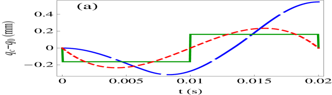
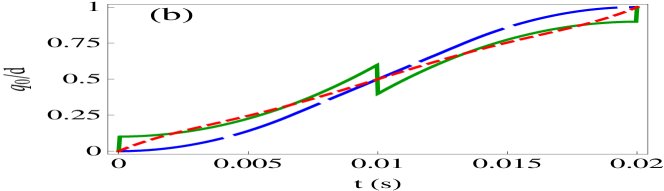
Figure 1: (Color online) (a) Displacement $q_{c}-q_{0}$ versus time. Blue long dashed line: direct method, red short dashed line: inverse method (polynomial). Solid green line: inverse method + OCT. (b) Trap trajectories. Parameter values: $d=1.6$ mm, $t_{f}=20$ ms, $\delta\simeq 0.162$ mm, $\omega_{0}=2\pi\cdot 50$ Hz.

To solve Eq. (8) we proceed in two different ways, using direct or inverse approaches.

In the direct approach we fix first the evolution of the center of the trap $q_{0}(t)$. In H_Nature , for example, see Fig. 5 there, $\dot{q}_{0}(t)$ is increased linearly during a quarter of the transported distance $d/4$, then kept constant for $d/2$, and finally ramped back to zero during the last quarter,

$$q_{0}(t)=\left\{\begin{array}[]{ll}{\frac{v_{m}^{2}t^{2}}{d}},&0<t<\frac{d}{2v_{m}}\\ v_{m}t-\frac{d}{4},&\frac{d}{2v_{m}}<t<\frac{d}{v_{m}}\\ \frac{v_{m}}{2(d/v_{m}-t_{f})}(t-t_{f})^{2}+d,&\frac{d}{v_{m}}<t<t_{f}\end{array}\right.,$$

where $v_{m}=3d/(2t_{f})$ is the maximum trap velocity during the transport compatible with $q_{0}(t_{f})=d$ in this scheme. Solving Eq. (9) for the previous $q_{0}(t)$ with initial conditions $q_{c}(0)=\dot{q}_{c}(0)=0$, and imposing continuity on $q_{c}(t)$ and $\dot{q}_{c}(t)$ we find

$$q_{c}(t_{f})\!-\!q_{0}(t_{f})\! = \!{9d}(1-2\cos\phi)(\sin^{2}\phi)/(\omega_{0}^{2}t_{f}^{2}),$$

$$\dot{q}_{c}(t_{f})\!-\!\dot{q}_{0}(t_{f})\! = \!\frac{9d}{2\omega_{0}t_{f}^{2}}(\sin\phi+\sin 2\phi-\sin 3\phi),$$ (12)

where $\phi=\omega_{0}t_{f}/3$. The final state of the transported BEC is given by Eqs. (7) and (12). In general some excitation is produced, except for the discrete set of final times $t_{f,N}=3(2N+1)\pi/\omega_{0}$, $N=0,1,2,...$, for which

$$q_{c}(t_{f})=d,\quad\dot{q}_{c}(t_{f})=\ddot{q}_{c}(t_{f})=0,$$ (13)

and the transported state matches the eigenstate of the final Hamiltonian. The classically moving center of mass and the trap center stop at $d$, $\dot{q}_{c}(t_{f})=0$, $\dot{q}_{0}(t_{f})=0$, with zero (classical) energy $m\dot{q}_{c}(t_{f})^{2}/2+m\omega_{0}^{2}[d-q_{c}(t_{f})]^{2}/2=0$. Using this direct approach, the minimum final time which does not produce excitation is $t_{f,0}=3\pi/\omega_{0}$ ($N=0$). In our example, $t_{f,0}=30$ ms. For such short times the transport is not adiabatic.

Thanks to the structure of the solution (7), we may apply a generalized inverse engineering method similar to the one for the linear case MCh ; ChPRL1 ; transport . The idea is to design $q_{c}(t)$ first and deduce the transport protocol from it. We impose the conditions (10) and (13) at $t=0$ and $t_{f}$, and interpolate $q_{c}$ with a function, e.g. a polynomial with enough parameters to satisfy all these conditions. Then $q_{0}(t)$ is calculated via Eq. (9). An example is shown in Fig. 1 where we have chosen $t_{f}=20$ ms $<t_{f,0}$. By construction no final excitation is produced, and the final fidelity (overlap between the transported state and the ground state at $t_{f}$) is one. Contrast this to the direct approach which, for $t_{f}=20$ ms, produces more transient excitation and a final excited state with nearly zero fidelity.

In principle there is no lower limit to $t_{f}$ with the inverse method, but in practice there are some limitations transport . Smaller values of $t_{f}$ increase the distance from the condensate to the trap center, see Eq. (12), and the effect of anharmonicity. There could be also geometrical constraints: for short $t_{f}$, $q_{0}(t)$ could exceed the interval [$0,d$]. For the polynomial ansatz this happens transport at $t_{f}=2.505/\omega_{0}$, $t_{f}\approx 8$ ms for the parameters of the example. Optical Control Theory (OCT) combined with the inverse method, see below, provides a way to design trajectories taking these restrictions into account.

Anharmonic Transport.—The inverse method can also be applied to anharmonic transport by means of a compensating force transport . To this aim, we consider a generic potential $U(q-q_{0})$ and set $\alpha(t)=q_{0}(t)$, $\omega(t)=\omega_{0}=0$, $f=0$, and $F=m\ddot{q}_{0}$ in Eq. (1), so the GPE becomes

$$i\hbar\frac{\partial\psi(q,t)}{\partial t}=\bigg{[}-\frac{\hbar^{2}}{2m}\nabla^{2}_{q}-m\ddot{q}_{0}q+U(q-q_{0})$$

$$+g_{{}_{1}}|\psi(q,t)|^{2}\bigg{]}\psi(q,t),$$

and the auxiliary equations (2) and (3) are satisfied trivially. Here we impose $q_{0}(0)=0,\quad\dot{q}_{0}(0)=0$, $q_{0}(t_{f})=d,\quad\dot{q}_{0}(t_{f})=0$. We may optionally impose also $\ddot{q}_{0}=0$ at $t=0$ and $t_{f}$. The function that must be interpolated is now $q_{0}(t)$, and again we consider a polynomial. For an arbitrary trap and $t_{f}=20$ ms, the maximal compensating acceleration would be $23.1$ m/s².

Optimal control theory.—Given the freedom left by the inverse method it is natural to combine it with OCT and design the trajectory according to relevant physical criteria stef . For harmonic transport, we have imposed the boundary conditions (10) and (13) at $t=0$ and $t_{f}$, but $q_{0}(t)$, and the polynomial ansatz for $q_{c}(t)$ are quite arbitrary. As an example of the possibilities of OCT suppose that we wish to limit the deviation of the condensate from the trap center according to $-\delta\leq q_{c}-q_{0}\leq\delta$, $\delta>0$ and find the minimal time $t_{f}$. The transport process given by Eqs. (7), (10) and (13) can be rewritten as a minimum-time optimal control problem defining the state variables $x_{1}(t)$ and $x_{2}(t)$ and the control $u(t)$,

$$x_{1}=\alpha,\quad x_{2}={\dot{\alpha}},\quad u(t)=\alpha-q_{0}.$$ (14)

Equation (9) is transformed into a system of equations,

$$\dot{x}_{1}=x_{2},\quad\dot{x}_{2}+\omega_{0}^{2}u=0.$$ (15)

The OCT problem is to find $-\delta\leq u(t)\leq\delta$ with $u(0)=u(t_{f})=0$, $\{x_{1}(0),x_{2}(0)\}=\{0,0\}$, and $\{x_{1}(t_{f}),x_{2}(t_{f})\}=\{d,0\}$ in the minimum final time $t_{f}$. The optimal control Hamiltonian LSP is $H_{c}=p_{1}x_{2}-p_{2}\omega_{0}^{2}u$, where $p_{1}$ and $p_{2}$ are conjugate variables. The Pontryagin maximality principle LSP tells us that for $u(t)$, $\mathbf{x}(t)$ to be time-optimal, it is necessary that there exists a nonzero, continuous vector $\mathbf{p}(t)$ such that $\mathbf{\dot{x}}=\partial H_{c}/\partial\mathbf{p}$, $\mathbf{\dot{p}}=-\partial H_{c}/\partial\mathbf{x}$ at any instant, the value of the control maximizes $H_{c}$, and $H_{c}(\mathbf{p}(t),\mathbf{x}(t),\mathbf{u}(t))=c\geq 0$, with $c$ a constant. The solution is of bang-bang type Salamon09 ,

$$u(t)=\left\{\begin{array}[]{ll}0,&t=0\\ -\delta,&0<t<t_{1}\\ \delta,&t_{1}<t<t_{f}\\ 0,&t=t_{f}\end{array}\right.,$$

where the initial and final discontinuities are chosen to satisfy the boundary conditions. Solving the system (15) and imposing continuity on $x_{1}$ and $x_{2}$ one finds for the switching and final times $t_{1}={t_{f}}/{2}$, $t_{f}={2}({d}/{\delta})^{1/2}/{\omega_{0}}$. The trap trajectory is deduced from Eq. (14),

$$q_{0}(t)=\left\{\begin{array}[]{ll}0,&t=0\\ ({1+\omega_{0}^{2}t^{2}}/{2})\delta,&0<t<t_{1}\\ -\big{[}{\omega_{0}^{2}}(t-t_{f})^{2}/2+1\big{]}\delta+d,&t_{1}<t<t_{f}\\ d,&t=t_{f}\end{array}\right..$$

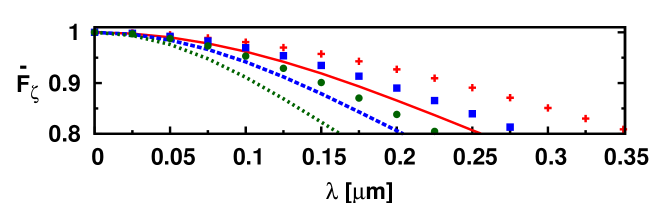
Figure 2: (Color online) Average fidelity of harmonic transport versus noise amplitude $\lambda$. For $t_{f}=20$ ms: $g_{{}_{1}}/\hbar=0.05\,m/s$ (solid, red line), $g_{{}_{1}}/\hbar=0.1\,m/s$ (dashed, blue line), $g_{{}_{1}}/\hbar=0.2\,m/s$ (dotted, green line); for $t_{f}=10$ ms: $g_{{}_{1}}/\hbar=0.05\,m/s$ (red crosses), $g_{{}_{1}}/\hbar=0.1\,m/s$ (blue boxes), $g_{{}_{1}}/\hbar=0.2\,m/s$ (green circles). $\omega_{0}=2\pi\cdot 50$ Hz.

In Fig. 1 the displacement of the center of mass with respect to the trap center and the trap trajectory are plotted for this optimal trajectory. We have chosen $\delta\simeq 0.162$ mm so that the minimal final time is $t_{f}=20$ ms as in the previous example.

Another important constraint might be that the center of the physical trap stays inside a given range (e.g. inside the vacuum chamber), i.e. the constraint is then $q_{\downarrow}\leq q_{0}(t)\leq q_{\uparrow}$. Following the OCT procedure we finally get

$$q_{0}(t)=\left\{\begin{array}[]{ll}0,&t=0\\ q_{\uparrow},&0<t<t_{1}\\ q_{\downarrow},&t_{1}<t<t_{f}\\ d,&t_{f}<t\end{array}\right.,$$

where $\omega_{0}t_{1}=\arccos\left[1-{q_{\downarrow}d-{d^{2}\over 2}\over q_{\uparrow}(q_{\downarrow}-q_{\uparrow})}\right]$, $\omega_{0}t_{f}=\omega_{0}t_{1}+\arccos\left\{[{q_{\downarrow}d-{d^{2}\over 2}-q_{\downarrow}(q_{\downarrow}-q_{\uparrow})]/[(d-q_{\downarrow})(q_{\downarrow}-q_{\uparrow})}]\right\}.$

Noise.—In the following we investigate the effect of noise in harmonic transport. We assume that the center of the physical trap is randomly perturbed by the shift $\lambda\zeta(t)$ with respect to $q_{0}(t)$. For the shifted trap center, Eq. (9) can be solved using the ansatz $\tilde{q}_{c}(t)=q_{c}(t)+\lambda\beta(t)$ so that $\beta(t)=\int_{0}^{\omega_{0}t}d\tau\,\zeta(\tau)\sin\left(\omega_{0}t-\tau\right)$, and $\dot{\beta}(t)=\omega_{0}\int_{0}^{\omega_{0}t}d\tau\,\zeta(\tau)\cos\left(\omega_{0}t-\tau\right)$, with the solution still given by Eq. (7). The fidelity at $t_{F}$ is independent of the chosen $q_{c}$ and $d$, ${F}_{\zeta}=\left|\int dq\,\exp\left(\frac{im}{\hbar}\lambda\dot{\beta}(t_{F})q\right)\chi^{*}(q+\lambda\beta(t_{F}))\chi(q)\right|$. We assume now that $\zeta(t)$ is white Gaussian noise, and average the fidelity ${F}_{\zeta}$ over different realizations of $\zeta(t)$. The result can be seen in Fig. 2 for three values of $g_{{}_{1}}$ and two final times, $t_{f}=20$ ms and $t_{f}=10$ ms. The fidelity increases for smaller couplings $g_{{}_{1}}$ and for the shorter time.

Outlook—The above results may be extended to other physically motivated constraints, also to non-spherical traps with different frequencies $\omega_{x}$, $\omega_{y}$, $\omega_{z}$, rotations, and launching/stopping condensates up to/from a determined velocity.

We thank D. Guéry-Odelin for discussions. We acknowledge funding by the Basque Government (Grant No. IT472-10) and Ministerio de Ciencia e Innovación (FIS2009-12773-C02-01). E. T. acknowledges financial support from the Basque Government (Grant No. BFI08.151); X. C. from Juan de la Cierva Programme and the National Natural Science Foundation of China (Grant No. 60806041); S. S. from the German Academic Exchange Service (DAAD).

References

(1) T. L. Gustavson et al.,
Phys. Rev. Lett. 88, 020401 (2002).
(2)W. Hänsel et al.,
Nature 413, 498-501 (2001).
(3) S. Schmid et al., New J. Phys. 8, 159 (2006).
(4)D. Xiong et al.,
Opt. Exp. 18, 1649 (2010).
(5) A. Couvert et al.,
Eur. Phys. Lett. 83, 13001 (2008).
(6)M. Murphy et al.,
Phys. Rev. A
79, 020301(R) (2009).
(7) S. Masuda and K. Nakamura, Proc. R. Soc. A
466, 1135 (2010).
(8)E. Torrontegui et al.,
Phys. Rev. A 83, 013415 (2011).
(9)X. Chen et al.,
Phys. Rev. Lett. 104, 063002 (2010).
(10) J. F. Schaff et al.,
Phys. Rev. A 82, 033430 (2010).
(11)J. G. Muga et al., J. Phys. B: At. Mol. Opt. Phys. 42 241001 (2009).
(12)J. F. Schaff et al.,
Eur. Phys. Lett. 93, 23001 (2011).
(13)A. del Campo, arXiv:1010.2854.
(14) H. R. Lewis and P. G. Leach, J. Math. Phys. 23, 2371 (1982).
(15) M. A. Lohe, J. Phys. A: Math. Theor. 42, 035307 (2009).
(16) H. R. Lewis and W. B. Riesenfeld, J. Math. Phys. 10, 1458 (1969)
(17) A. K. Dhara and S. W. Lawande,
J. Phys. A 17, 2423 (1984).
(18)W. Hänsel et al.,
Phys. Rev. Lett. 86, 608 (2001).
(19) A. Günther et al.,
Phys. Rev. 71, 63619 (2005).
(20) F. Dalfovo, S. Giorgini, L. P. Pitaevskii, and S.
Stringari, Rev. Mod. Phys. 71, 463 (1999).
(21) D. Stefanatos, J. Ruths, and Jr-Shin Li,
Phys. Rev. A 82, 063422 (2010).
(22) L. S. Pontryagin et al., The Mathematical Theory of Optimal Processes
(Interscience Publishers, New York, 1962).
(23) P. Salamon et al.,
Phys. Chem. Chem. Phys. 11, 1027
(2009).