Synthesizing attractors of Hindmarsh-Rose neuronal systems

Abstract

In this paper a periodic parameter switching scheme is applied to the Hindmarsh-Rose neuronal system to synthesize certain attractors. Results show numerically, via computer graphic simulations, that the obtained synthesized attractor belongs to the class of all admissible attractors for the Hindmarsh-Rose neuronal system and matches the averaged attractor obtained with the control parameter replaced with the averaged switched parameter values. This feature allows us to imagine that living beings are able to maintain vital behavior while the control parameter switches so that their dynamical behavior is suitable for the given environment.

keywords: Hindmarsh-Rose model; chaotic attractors; local attractors; global attractors

Figure 1: (a) Bifurcation diagram: $x_{1}$ vs $p$ with $I=3.4$. (b) Detail of Fig. 1a. (c) Consecutive detail of Fig. 1b. (d) Bifurcation diagram: $x_{1}$ vs $p$ with $I=3.5.$

1 Introduction

Based on the theory of dynamical systems, Hindmarsh and Rose proposed the phenomenological neuron model, which may be seen either as a generalization of the Fitzhugh equations or as a simplification of the physiologically realistic model proposed by Hodgkin and Huxley [1, 2]. The Hindmarsh-Rose (HR) model of neuronal activity is aimed to study the spiking-bursting behavior of the membrane potential observed in experiments of a cell in the brain of the pond snail [1]. The dynamics of a single HR neuron has been studied well, and it is illustrated that it can exhibit complex dynamical behavior including periodic and chaotic spiking (bursting) motion when certain control parameters of nervous cell models are varied [1, 2, 3].

It is well accepted that the HR neuron model is an alternative candidate for studying the dynamics of neuronal systems since it has simpler mathematical forms than Chay’s and Hodgkin and Huxley’s neuron models [4, 5]. Therefore, this model has been used to study different aspects of neuronal dynamics such as transitions between different firing regimes [6], relations between block structured dynamics and neuronal coding [7], the effect of noise on neuronal signal transduction [8] and on synchronization [9], the collective dynamics of neuronal networks [10] and the evolution of spiral waves in coupled Hindmarsh-Rose neurons [11].

However, an important phenomenon in neuron activity is the transition between different firing patterns. From the viewpoint of dynamical systems, it is crucial to investigate the transition mechanism of firing patterns for understanding realistic neuronal activities. The local stability and the numerical asymptotic analysis of the Hindmarsh-Rose model are used to investigate the firing evolution of a single Hindmarsh-Rose neuron [12]. A simple one-dimensional map method has been applied to the HR neurons to convert irregular spiking and chaotic bursting to regular beating and periodic bursting [13].

Recently, we developed a parameter switching method to synthesize attractors of a class of dynamical systems, called hereafter attractors synthesis (AS) algorithm. This method in fact starts from a set of given parameter values, and allows us, via periodic or random parameter-switching, to generate any of the set of all possible attractors of a class of continuous time dynamical systems of integer order[14],[15], or of fractional order [16], depending linearly on the control parameter. It has been applied successfully to several dynamical systems such as Lorenz, Chen, Rössler, Lotka-Volterra, minimal networks, fractional Lü systems and so on. Extending this subject, we will synthesize attractors of the HR neuronal model, which can exhibit burst dynamics, via the AS method contributing to a better understanding of neuronal firing transition.

The paper is organized as follows: the HR model will be described in Sec. 2; the AS method will be introduced in Sec. 3, and attractors will be synthesized in Sec. 4. Finally, the paper will end in Sec. 5 with some comments and conclusions.

2 Description of Hindmarsh-Rose model

The dynamics of an isolated HR neuron is governed by the following set of differential equations [1]:

$$\begin{array}[c]{cl}\overset{\cdot}{x}_{1}=&bx_{1}^{2}-ax_{1}^{3}+x_{2}-x_{3}+I,\\ \overset{\cdot}{x}_{2}=&c-dx_{1}^{2}-x_{2},\\ \overset{\cdot}{x}_{3}=&p[s(x_{1}-\overline{x}_{1})-x_{3}],\end{array}$$ (1)

where $x_{1}$ is the membrane potential, $x_{2}$ is associated with the fast current, Na⁺, or K⁺ and $x_{3}$ with the slow current, for example, Ca²⁺. The parameters are [1]: $a=1,~{}b=3,~{}c=1,~{}d=5,$ $s=4$,  $\overline{x}_{1}=-1/2(1+\sqrt{5)}\simeq-1.6$. $I$ and $p$ are the control parameters, and $I~{}$is a slow parameter while $p~{}$is a fast parameter. $I$ mimics the membrane input current for biological neurons; $p$ controls the speed of variation of the slow variable.

To find the fixed points we have to solve numerically the following equations: $x_{2}=-5x_{1}^{2}+1,$  $x_{3}=4x_{1}+6.4$, and $x_{1}^{3}+2x_{1}^{2}+4x_{1}+2=0$ which gives the single real solution $x_{1}=-0.639,~{}x_{2}=-1.041,~{}x_{3}=3.8442.$ Therefore the system (1) has a single equilibrium point: $X^{\ast}=\left(-0.639,-1.041,3.844\right)^{T}$

Parameter $p~{}$ is the ratio of time scales between fast dynamics and slow dynamics. Therefore, it controls the difference between the slow and the fast dynamics of HR neuron model corresponding to the difference between fast fluxes of ions across the membrane and slow ones. Therefore, it is really interesting to investigate the dynamics of the HR neuron as the parameter $p~{}$is changed. However, with $I$ as control parameter, the underlying dynamical system does not belong to the class of systems where AS can be applied [see Section 3].

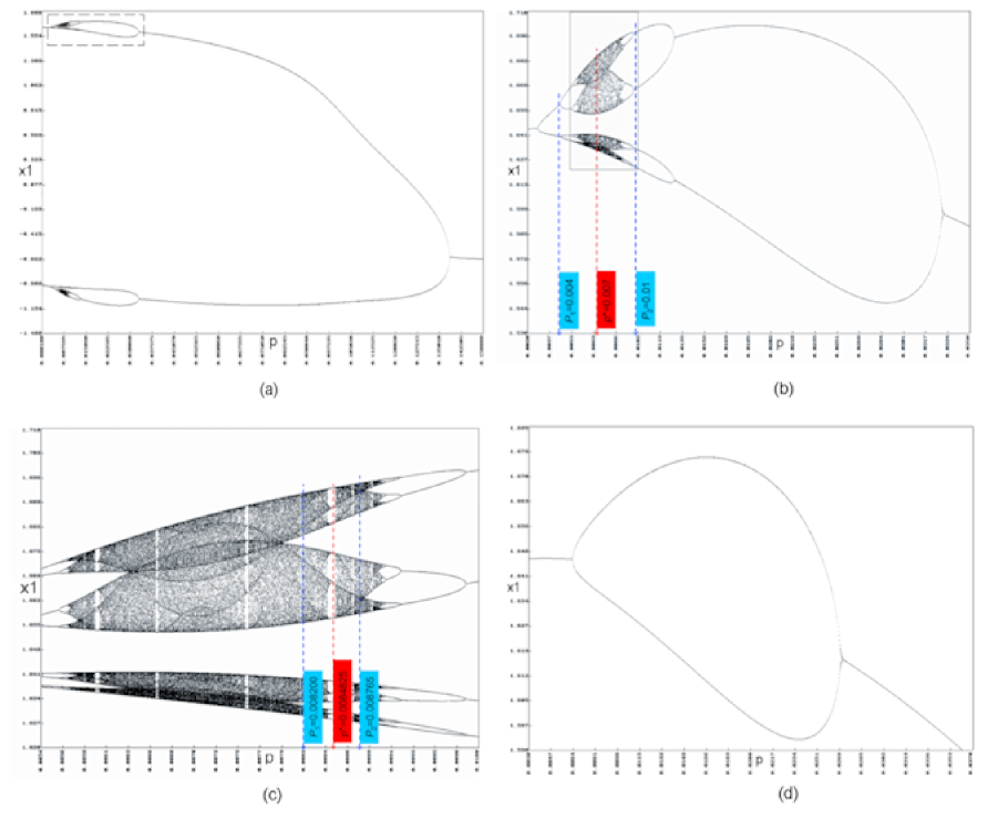
The bifurcation diagram of the first component $x_{1}$ versus $p~{}$ is shown in Fig. 1a,b,c for $I=3.4$, while that for $I=3.5$ in Fig. 1d. We are interested in the case $I=3.4$ because this case represents interesting dynamics, where chaos appears in a narrow range of $p$ with a width of about $3.5\times 10^{-3}$. Fig. 1a gives the bifurcation diagram with respect to the control parameter $p~{}$ in the range [0.0001, 0.15]. It is shown that as the parameter $p~{}$ is changed, the HR neuron firstly bifurcates from period-doubling to chaos, and then, it is stopped via the inverse period-doubling. For a clear vision, the enlargement of Fig. 1a is shown in Fig. 1b, which further confirms the above observation. Further enlargement can clearly guide our assessment as illustrated in Fig. 1c.

More details on the dynamics of the HR model can be found in [12]

3 Attractors synthesis algorithm

The AS algorithm can be applied to the following general class of continuous-time autonomous and dissipative dynamical systems, modeled by the Initial Value Problem (IVP) [15]

$$~{}S:~{}\dot{x}=f_{p}(x),\quad x(0)=x_{0},$$ (2)

where $f_{p}\,$ is an $\mathbb{R}^{n}$-valued function with a bifurcation parameter $p\in\mathbb{R}$, $n\geq 3$, and has the expression

$$f_{p}(x\mathbf{)=}g(x\mathbf{)}+pAx,$$ (3)

$g:\mathbb{R}^{n}\longrightarrow\mathbb{R}^{n}~{}\$is a continuous-time nonlinear function, $A~{}$is a real constant $n\times n$ matrix,$~{}x_{0}\in\mathbb{R}^{n}$, and $t\in[0,T).$

This class of dynamical systems contains the best-known systems such as Lorenz, Chen, Rössler, Lotka-Volterra, minimal networks, fractional Lü systems and so on (see [14][15][16]).

In [15] it has been shown, via numerical analysis and computer graphic simulations, that the AS algorithm allows the synthesis of any attractor of $S$ by parameter switching following some designed rule.

The AS algorithm can explain what happens with a system when, intentionally or not, the parameter value switches quickly through a set of values. Thus, when $p$ is switched following some designed deterministic [15] or random [14] rule, while the system evolves in time, an attractor belonging to the set of attractors is generated (synthesized).

The AS algorithm can be useful in the cases where some desired control parameter value cannot be directly accessed and we want to obtain the corresponding attractor.

Let us next suppose the following assumptions hold.

Assumption A.1. Throughout, the existence and uniqueness of solutions of the IVP (2)-(3) are assumed.

As known, the computer graphic simulations of the numerical integration results of (2)-(3) can give excellent approximations to the orbits within the invariant sets [17]. Thus, the orbits which start near a hyperbolic attractor will stay near and they will be shadowed by orbits within the attractor. This happens because attractors arise as the limiting behavior of orbits. Therefore, the shadowing property of hyperbolic sets [18] enables us to recover long time approximation properties of numerical orbits such as HR’s case.

The AS algorithm consists in using a time varying, or more precisely, a periodically switching parameter, according to some design rule. It will be shown, empirically by various experiments, that a desired targeted attractor can be duly obtained by the proposed switching scheme.

Remark 1

The algorithm is robust to some extent: the switching timing and switching parameter values both allow flexibility. Therefore, they do not need to be very precisely determined.

Hereafter the following notations will be used

Notation 1

Let us denote by $\mathcal{A}$ the set of all global attractors of $S$, including attractive stable fixed points, limit cycles and chaotic (possibly strange) attractors; $\mathcal{P\subset}\mathbb{R}$ the ordered set of the corresponding admissible values of $p$ and $\mathcal{P}_{N}=\{p_{1},p_{2},\ldots,p_{N}\}\subset$ $\mathcal{P}\,$ a finite ordered subset of $\mathcal{P}$ containing $N$ different values $p$, which determines the set of attractors $\mathcal{A}_{N}=\{A_{p_{1}},A_{p_{2}},\ldots,A_{p_{N}}\}\subset\,\mathcal{A}$.

Assumptions

A.2. $\mathcal{P}$ is considered, as in most cases, to be composed of a single real interval and all the values of $\mathcal{P}_{N}=\{p_{1},p_{2},\ldots,p_{N}\}~{}$for which the system behaves stable and/or chaotic is assumed to be accessible.

A.3. $S$ is dissipative i.e. $\bigtriangledown\cdot f<0,$ where $\bigtriangledown\cdot f\equiv\sum\limits_{i=1}^{n}\partial f\left(x_{1},x_{2},\ldots,x_{n}\right)/\partial x_{i}$ (see e.g. [19]).

Due to the assumed dissipativity, $\mathcal{A}$ is non-empty and it follows naturally that for the considered class of systems, a bijection may be defined between the sets $\mathcal{P}$ and $\mathcal{A}$. Thus, giving any $p\in\mathcal{P}$, a unique global attractor is specified, and vice versa.

Remark 2

Because in this paper computer simulations are used as the major analytical tool, the $\omega$-limit set (actually, its approximation [20]) is considered after neglecting a sufficiently long period of transients. Therefore, by attractors (background on the notion of attractor can be found in [21]) it is appropriate to understand in this paper the $\omega$-limit set obtained by a numerical method for ODEs with fixed step size $h$ after the transients were neglected.

Let $\mathcal{P}_{N}=\{p_{1},p_{2},\ldots,p_{N}\}.$ The AS algorithm relies on the following deterministic time rule applied repeatedly on $I$

$$[(m_{1}h)p_{1},~{}(m_{2}h)p_{2},\ldots,(m_{N}h)~{}p_{N}],$$ (4)

where the weights $m_{i}~{}$are some positive integers. The algorithm acts as follow: in the first time subinterval of length $m_{1}h$, $p$ will have the value $\ p_{1}~{}$(i.e. the IVP(2)-(3) will be integrated $m_{1}$ steps for $p=p_{1}$), for the next $m_{2}$ integration steps, $p=p_{2}$ and so on until the $N$-th time subinterval of length $m_{N}h$ where $p=p_{N}$ and then the algorithm repeats. In order to simplify the notation in (4), for a fixed step size $h$, the scheme (4) will be denoted next

$$[m_{1}p_{1},~{}m_{2}p_{2},\ldots,m_{N}~{}p_{N}].$$ (5)

For example, the scheme $\left[p_{3},3p_{1},2p_{2}\right]$ represents the infinite sequence of $p:$ $p_{3},3p_{1},2p_{2},p_{3},3p_{1},2p_{2},\ldots~{}\ \$which means that while the considered numerical method integrates (2)-(3), $~{}p$ switches in each $m_{i}h$ time subinterval. In other words, the numerical method will integrate (2)-(3) one step with $p=p_{3},$ then three times with $p=p_{1},$ then two steps with $p=p_{2}$ and so on.

The AS algorithm for the scheme (5) is presented in Fig. 2

$$\begin{array}[c]{l}t=0\\ repeat\\ ~{}\ \ \ \ for\quad k=1~{}to~{}N~{}do\\ ~{}\ \ \ \ \ \ \ \ \ \ p=p_{k}\\ ~{}~{}~{}~{}~{}~{}~{}~{}~{}~{}\ for~{}i=1~{}to~{}m_{k}~{}do\\ ~{}~{}~{}\ ~{}~{}~{}~{}~{}~{}~{}~{}~{}~{}~{}~{}~{}integrate~{}(\ref{IVPa})-(\ref{IVPb})\\ ~{}~{}~{}~{}~{}~{}~{}~{}~{}~{}~{}~{}~{}~{}~{}~{}~{}t=t+h\\ ~{}~{}~{}~{}~{}~{}~{}~{}~{}~{}~{}end\\ ~{}~{}~{}~{}~{}end\\ until~{}t\geq T\end{array}$$

Figure 2: Pseudocode of AS algorithm.

Notation 2

Let us denote the synthesized attractor obtained with AS algorithm, via (5), by $A^{\ast}~{}$and by $A_{p^{\ast}}$ the averaged attractor corresponding to

$$p^{\ast}=\frac{\sum\limits_{k=1}^{N}p_{k}m_{k}}{\sum\limits_{k=1}^{N}m_{k}}.$$ (6)

Next, the following notion is introduced

Definition 1

Two attractors are considered to be identical if their underlying $\omega$-limit sets coincide in the phase space, the identity being considered from a geometric point of view in the phase space, aided by computer graphic analysis.

This identity in the case of chaotic attractors will be considered only asymptotically since they are fully depicted only after an infinite time.

Proposition 1

The synthesized attractor $A^{\ast}$ and the averaged attractor $A_{p^{\ast}}$ are identical

Proof. Let us consider some subset $\mathcal{P}_{N}$. If we denote $\alpha_{k}=m_{k}/\sum\limits_{i=1}^{N}m_{i},$ it is easy to see that $p^{\ast}$ is a convex combination $p^{\ast}=\sum\limits_{k=1}^{N}\alpha_{k}p_{k},$ since $\ \sum\limits_{k=1}^{N}\alpha_{k}=1.$ Therefore $p^{\ast}$ belongs within the interval $\left(p_{1},\ldots,p_{N}\right)$, whatever the values $p_{i}$ are chosen. Also, taking into account the bijection between $\mathcal{P}$ and $\mathcal{A}$, we are entitled to consider that the same convex structure is preserved into $\mathcal{A}.$ Therefore, for whatever switched values of $p$ in some subset $\mathcal{P}_{N}$, $A^{\ast}$ will belong within the set $\mathcal{A}_{N}$  considered to be ordered by the mentioned bijection i.e. $A_{p^{\ast}}\in\left(A_{p_{1}},A_{p_{N}}\right)$.  Next, aided by numerical analysis and via computer graphics, it can be showed that $A^{\ast}$ is identical (in the sense defined above) to $A_{p^{\ast}}.$Therefore $A^{\ast}\in\left(A_{p_{1}},A_{p_{N}}\right).$   

Next, we can formulate the main property of the AS algorithm

Proposition 2

For whatever considered set $\mathcal{P}_{N}$, the AS algorithm generates an attractor $A^{\ast}~{}$which belongs to $\left(A_{p_{1}},A_{p_{N}}\right).$

Remark 3

The AS algorithm is useful especially when we want to obtain some attractor $\overline{A}_{\overline{p}}~{}$even the underlying value $\overline{p}~{}$cannot be accessible.

In this case $\overline{A}$ can be synthesized by choosing a corresponding set $\left(p_{1},\ldots,p_{N}\right)\ni\overline{p}$ but $\overline{p}\notin\mathcal{P}_{N}=\{p_{1},\ldots,p_{N}\},$ and a corresponding scheme (5).

The initial conditions play an important role since for a specific value $p\in\mathcal{P}$ there is a single global attractor but which could be composed by several local attractors (see e.g. [21],[22],[23],[24]). For example, for the Lorenz system for the control parameter $r=2.5$ there are three local attractors: the origin and two symmetrical fixed points $X_{1},_{2}(\pm 2,~{}\mp 2,~{}1.5$) while for $r=28$ there is a single local attractor which is global too, the known Lorenz strange attractor. To avoid these possible difficulties, all the computer simulations for $A^{\ast}$ and $A_{p^{\ast}}$ for a particular case, start from the same initial conditions.

Figure 3: AS algorithm with scheme $[1p_{1},1p_{2}]$ with $p_{1}=0.004$ and $p_{2}=0.01;$ a) The synthesized and averaged attractors $A^{\ast}$ and $A_{p^{\ast}}~{}$respectively, superimposed for $p^{\ast}=0.007~{}$; b) Attractor $A_{0.004\text{ }};$ c) Attractor $A_{0.01}.$

In order to see how the AS algorithm works, let us consider that we want to synthesize the attractor $\overline{A}_{\overline{p}}.$

Then we must choose $N$ and the set $\mathcal{P}_{N}$ such that $\overline{p}\in\left(p_{1},\ldots,p_{N}\right)$ ( $\overline{p}~{}$can be equal or not to one of the elements $p_{i},$ for $i=2,\ldots N-1).$ Next, choosing empirically the scheme (5), such that the right-hand side of (6) gives $\overline{p},$ the initial value problem is integrated and finally $\overline{A}_{\overline{p}}$ is obtained.

To underline the identity between $A^{\ast}$ and $A_{p^{\ast}}~{}$histograms and Poincaré sections besides the phase plots were drawn after the transients were neglected.

Figure 4: AS algorithm for $N=10,$ $p_{i}=0.0002+i\times 0.0001~{}$and $m_{i}=1,$ for $i=1,2,\ldots,10;$ $A^{\ast}$ and $A_{p^{\ast}},~{}$with $p^{\ast}=0.00075,$ are superimposed.

4 Synthesis of HR attractors

Real neurons often display high nonlinearity, which has been shown in many experiments and confirmed by numerical simulation of many neuron models, including the HR and Chay neuron models[1, 4]. Chaos is a universal phenomenon in certain neurons, such as those in the human brain where, often, the information is decoded and transduced by means of chaos. It is very important to study the chaos of neuron from different aspects. Next, we will focus on the neuronal firing pattern when $p$ is switched.

Firstly, it is easy to prove the following

Proposition 3

The HR system (1) with $p$ considered as control parameter, belongs to the class of systems modeled by the IVP (2)-(3).

Proof. Choosing the following substitution

$$y_{1}=x_{1}-\overline{x}_{1}$$

and replacing finally $y_{1}$ with $x_{1},$ (1) becomes

$$\overset{.}{x}_{1} =a_{1}x_{1}^{3}+b_{1}x_{1}^{2}+c_{1}x_{1}+d_{1}x_{2}+e_{1}x_{3}+f_{1}+I,$$ (7)

$$\overset{.}{x}_{2} =a_{2}x_{1}^{2}+b_{2}x_{1}+c_{2}x_{2}+d_{2},$$

$$\overset{.}{x}_{3} =p(sx_{1}-x_{3}),$$

where

$$a_{1} =-a,$$

$$b_{1} =b-3a\overline{x}_{1},$$

$$c_{1} =\overline{x}_{1}\left(2b-3a\overline{x}_{1}\right),$$

$$d_{1} =1,$$

$$e_{1} =-1,$$

$$f_{1} =-a\overline{x}_{1}^{3}+b\overline{x}_{1}^{2},$$

$$a_{2} =-d,$$

$$b_{2} =-2d\overline{x}_{1},$$

$$c_{2} =-1,$$

$$d_{2} =d\overline{x}_{1}^{2}.$$

Thus, the right hand side of (7) can be written following (3) with

$$g(x)=\left(\begin{array}[c]{c}a_{1}x_{1}^{3}+b_{1}x_{1}^{2}+c_{1}x_{1}+d_{1}x_{2}+e_{1}x_{3}+f_{1}+I\\ a_{2}x_{1}^{2}+b_{2}x_{1}+c_{2}x_{2}+d_{2}\\ 0\end{array}\right)$$

$$\text{ }A=\left(\begin{array}[c]{ccc}0&0&0\\ 0&0&0\\ s&0&-1\end{array}\right)\text{ \rm and }x=\left(\begin{array}[c]{c}x_{1}\\ x_{2}\\ x_{3}\end{array}\right).$$

 

Figure 5: AS algorithm for $N=2$ and $\mathcal{P}_{N}=\{0.0082,0.008765\}$ and $m_{1}=m_{2}=1;$ a) $A^{\ast}$ and $A_{p^{\ast}},~{}$with $p^{\ast}=0.0084825~{},$ superimposed; b) $A_{0.0082};$ c) $A_{0.008765};$ d) Superimposed histograms of $A^{\ast}~{}$and $A_{p^{\ast}};$ e) Superimposed Poincaré sections of $A^{\ast}~{}$and $A_{p^{\ast}}~{}$for $\ x_{1}=1.2.$

Because, from a numerical point of view, the mathematical model (1) presents a more accessible form than (7), next we will work with (1).

The HR system verifies the assumptions A1, A2 and also A3 for large parameters range taking into account that $\bigtriangledown\cdot f=-3ax_{1}^{2}+2bx_{1}-1-p.$ Therefore, one can apply the AS algorithm to the HR system (1). For this purpose we considered the Standard Runge-Kutta numerical method for ODEs with the fixed step size $h=0.005$ and, as stated above, $I=3.4.$

Figure 6: Temporal evolution of Lyapunov exponents for $p=0.0084825.$

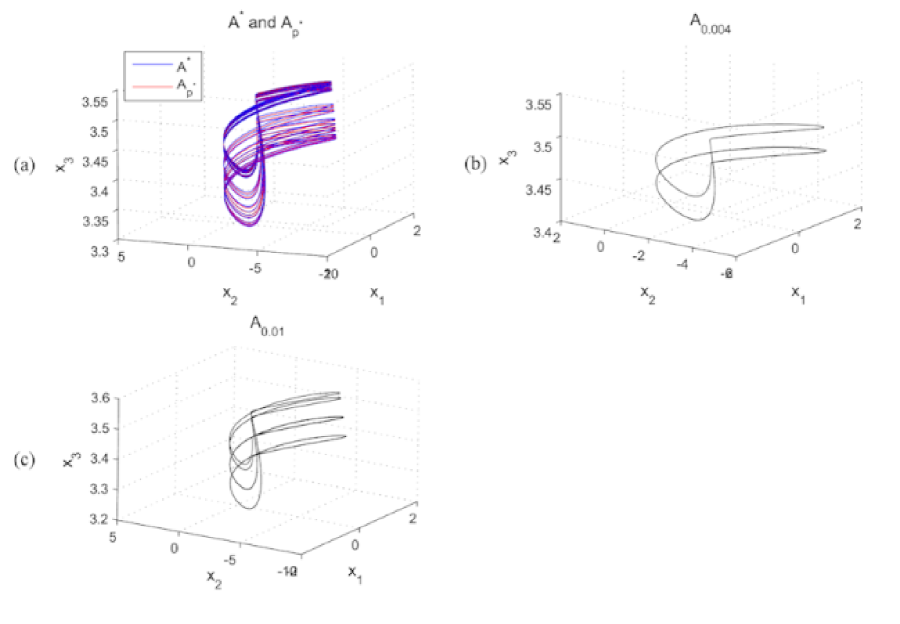
For the sake of the brevity, in what follows, only the most relevant cases are considered. Let us firstly consider the case $N=2$ and $\mathcal{P}_{N}=\{0.004,0.01\}$ (see Fig. 1b) with $m_{1}=m_{2}=1.$ Then, using the scheme $[1p_{1},1p_{2}]$ while integrating the initial value problem (1), finally, even the attractors $A_{0.004\text{ }}$and $\ A_{0.01}$ are stable limit cycles, the obtained synthesized attractor $A^{\ast}$ is chaotic (Fig. 3a). As can be seen from Fig. 3a, the synthesized attractor $A^{\ast}$ (blue) and the averaged attractor $A_{p^{\ast}}$ (red) for $p^{\ast}=(0.004+0.01)/2=0.007~{}$ given by (6) coincide. It can be seen that $p^{\ast}\in(p_{1},p_{2})$ (Fig. 1b) and also $A^{\ast}$ is situated between the corresponding attractors $A_{p_{1}}$ and $A_{p_{2}}.$

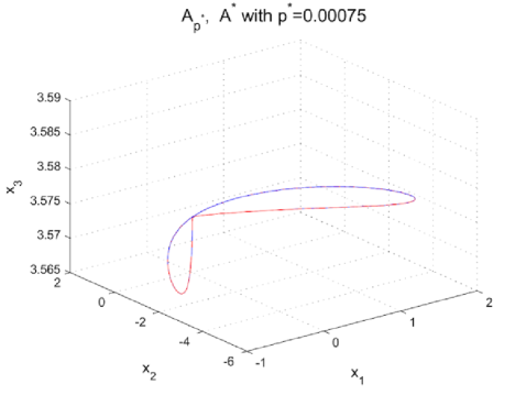
Next, if we use $N=10$ values for $p$ defined as follows: $p_{i}=0.0002+i\times 0.0001~{}$and $m_{i}=1,$ for $i=1,2,\ldots,10,$ the synthesized attractor $A^{\ast}$ is a stable limit cycle which coincides with the averaged attractor $A_{p^{\ast}}$ with $p^{\ast}=0.00075~{}$(Fig. 4).

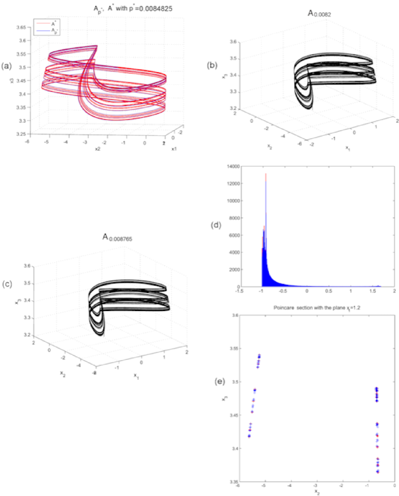
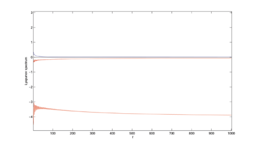
An interesting case appears for $N=2$ and $\mathcal{P}_{N}=\{0.0082,0.008765\}$ and $m_{1}=m_{2}=1,$ where $p_{1},$ and $p_{2}$ are chosen in a very narrow periodic window (its width is about $1E-~{}4~{}$, see Fig. 1c, Fig. 5b and Fig. 5c). The obtained attractor, $A^{\ast},$ is identical to $A_{p^{\ast}}$ for $p^{\ast}=0.0084825~{}$(Fig. 5 a). We found numerically that the fixed point $X^{\ast}~{}$is unstable for $p=p^{\ast}~{}$since the three eigenvalues are: $-6.266,0.179$ and $0.02$ and, as showed in Fig. 6, the Lyapunov spectrum has two negative exponents while the maximum one is positive (approximately zero). All these lead us to consider that $A_{p^{\ast}}$ (and consequently $A^{\ast})$ is a stable limit cycle. The apparent difference between the attractors in this case is due to the very small difference between $p_{1}$ and $p_{2}.$

5 Conclusions

In summary, we have investigated the synthesis of attractors of the HR neuronal system by means of the AS method. It is shown that when we choose the slow parameter $p~{}$ as the control parameter, the HR neuronal system belongs to a class of systems, where we can apply the proposed switching method. Consequently, we concluded that every attractor can be synthesized by the proposed periodic parameter switching scheme in the HR neuron model. It is accepted that neurons can code information by means of firing patterns, which depends on the variation of key parameters of neuronal systems. Hence, the results presented in this paper may be instructive in understanding the implications of realistic neuronal dynamics.

Acknowledgements    This work was supported by the National Science Foundation of China (Fund Nos. 10972001, 10702023 and 10832006).

References

- [1] Hindmarsh, J.L. and Rose, R.M.: A model of neuronal bursting using three coupled first order differential equations. Proc. R. Sc. Lond. B 221, 87-102 1984.
- [2] Ma, S.Q., Feng Z. and Lu, Q.S.: Dynamics and double Hopf bifurcations of the Rose-Hindmarsh system with time delay. Int. J. Bifurcation and Chaos 19, 3733-3751 2009.
- [3] Holden, A. V. and Fan, Y. S.: From simple to simple bursting oscillatory behavior via chaos in the Rose-Hindmarsh model for neuronal activity. Chaos, Solitons and Fractals 2(3), 221-236 1992.
- [4] Chay, T. R.: Chaos in a three-variable model of an excitable cell. Physica D 16(2), 233-242 1985.
- [5] Hodgkin, A. L. and Huxley, A. F.: A quantitative description of membrane current and its application to conduction and excitation in nerve. J Physiol. 117(4), 500–544 1952.
- [6] Gonzalez-Miranda, J. M.: Observation of a continuous interior crisis in the Hindmarsh-Rose neuron model. Chaos 13(3), 845-852 2003.
- [7] Gonzalez-Miranda, J.M.: Block structured dynamics and neuronal coding. Phys. Rev. E 72 (5), 051922 2005.
- [8] Reinker, S., Puil, E. and Miura, R. M.: Stochastic and suprathreshold resonances in a stochastic Hindmarsh-Rose model of thalamic neurons. Bull. Math. Biol. 65, 641-663 2003.
- [9] He, D., Shi, P. and L.: Stone, Noise-induced synchronization in realistic models. Phys. Rev. E 67, 027201 2003.
- [10] Zheng, Y. H. and Lu, Q. S.: Spatiotemporal patterns and chaotic burst synchronization in a small-world neuronal network. Physica A 387(14), 3719-3728 2008.
- [11] J. Ma, Y. Ja, J. Tang and Yang, J. L.: Breakup of spiral waves in coupled Hindmarsh-Rose neurons. Chin. Phys. Lett. 25, 4324-4328 2008.
- [12] Corson, N. and Aziz-Alaoui, M.A.: Asymptotic Dynamics of the slow-fast Hindmarsh-Rose neuronal system. (submitted)
- [13] Sabbagh, H.: Control of chaotic solutions of the Hindmarsh-Rose equations. Chaos, Solitons and Fractals 11(8), 1213-1218 2000.
- [14] Danca, M.-F.: Random parameter-switching synthesis of a class of hyperbolic attractors. Chaos 18, 033111 2008.
- [15] Danca, M.-F., Tang, W.K.S. and Chen, G.: A switching scheme for synthesizing attractors of dissipative chaotic systems. Applied Mathematics and Computations 201(1-2), 650-667 2008.
- [16] Danca, M.-F. and Diethlem, K.: Fractional-order attractors synthesis via parameter switchings. Communications in Nonlinear Science and Numerical Simulations DOI: 10.1016/j.cnsns.2010.01.011 (2010).
- [17] Stuart, A. M. and Humphries, A. R.: Dynamical Systems and Numerical Analysis. Cambridge University Press 1996.
- [18] Coombes, B., Kocak, H. and Palmer, K.: Rigorous computational shadowing of orbits of ordinary differential equations. Numer. Math. 69, 401-421 1995.
- [19] Ott, E.: Chaos in dynamical systems. Cambridge: Cambridge University Press) 1993.
- [20] Foias, C. and Jolly, M.S., 1995, On the numerical algebraic approximation of global attractors. Nonlinearity 8, 295–319.
- [21] Milnor, J.: On the concept of attractor. Communications in Mathematical Physics 99(2), 177–195 1985.
- [22] Hirsch, M. and Pugh, C.: 1970, Stable manifolds and hyperbolic sets. Proc. Symp. Pure Math. 14, American Mathematical Society, 133–164 1970.
- [23] Hirsch, M. W., Smale, S. and Devaney, R. L.: Differential Equations, Dynamical Systems and An Introduction to Chaos. second ed. (Elsevier Academic Press) 2004.
- [24] Kapitanski, L. and Rodnianski, I.: Shape and Morse theory of attractors. Communications on Pure and Applied Mathematics 53, 218–242 2000.