Phenomenological interpolation of the inclusive J/ cross section to proton-proton collisions at TeV and 5.5 TeV
Abstract
We present a study of the inclusive J/ cross section at TeV and TeV. The dependence of the cross section, rapidity and transverse momentum distributions are evaluated phenomenologically. Their knowledge is crucial as a reference for the interpretation of A–A and p–A J/ results at the LHC. Our approach is the following: first, we estimate the evolution of the -integrated J/ cross section at mid-rapidity; then, we evaluate the rapidity dependence; finally, we study the transverse momentum distribution trend. Whenever possible, both theory driven (based on pQCD predictions) and functional form (data driven fits) calculations are discussed. Our predictions are compared with the recently obtained results by the ALICE collaboration in pp collisions at 2.76 TeV.
1 Introduction
High energy heavy-ion collisions are used to study strongly interacting matter under extreme conditions. At sufficiently high collision energies, it is believed that hot and dense deconfined matter, commonly referred to as the Quark-Gluon Plasma (QGP), is formed. With the advent of a new generation of experiments at the CERN Large Hadron Collider (LHC) [1] a new energy domain is accessible to study the properties of such a state of matter. Many observables have been proposed to probe deconfined matter formed in heavy-ion collisions. The production of heavy-quarks and quarkonium at LHC energies is promising since their production rate allows now careful studies of their characteristics ( and distributions, polarization, flow, azimuthal correlations) [2, 3]. In particular, the production of charm is expected to be large enough to make regeneration mechanisms possible. The regeneration of J/ mesons due to the recombination of and quarks in later stage of the heavy-ion collision would be a direct probe of the deconfined QCD matter [4]. One of the experimental methods to quantify the nuclear medium effects in the production of a given observable () is the measurement of the nuclear modification factor () in nucleus-nucleus (A–A) collisions, defined as:
| (1) |
where is the average number of binary nucleon-nucleon collisions111 The average number of binary nucleon-nucleon collisions can be estimated by the product of the average nuclear overlap function (of the nucleus-nucleus collision) and the inelastic proton-proton cross section [5]. and () is the invariant yield of the observable in A–A (pp) collisions at a given (same) center-of-mass energy. In the absence of nuclear matter effects, the nuclear modification factor should be equal to unity for experimental observables commonly called hard probes (large particles, jets, heavy-flavour, etc). A similar factor , measured in p–A collisions, is crucial in order to disentangle hot and cold nuclear matter effects in A–A collisions.
First results on quarkonium production in proton-proton collisions at TeV have been published by the LHC experiments [6, 7, 8, 9] and a successful heavy-ion campaigns took place at the LHC in November 2010 and 2011, when Pb–Pb collisions at the energy per nucleon pair of TeV where delivered to the LHC experiments, for an integrated luminosity of about 9 b-1. The nominal LHC energies for pp and Pb–Pb collisions are TeV and TeV, respectively.
In this letter, we present an interpolation of the -integrated and differential inclusive J/ cross section in pp collisions to TeV and TeV. We establish a procedure to determine the J/ cross section at arbitrary energy values, which makes possible the calculation of the J/ nuclear modification factors for any colliding system and energy at the LHC222 As an example, the center-of-mass energy per nucleon pair in p–Pb collisions is 3.5–4 TeV at the present LHC energy, 7 TeV for pp collisions, and of 8.8 TeV at nominal energy. In the present LHC schedule, a p–Pb run is foreseen by the end of 2012. Operation at nominal energy will be commissioned after 2013. . The interpolation is done in three steps. The first step is an energy interpolation of the existing -integrated J/ production cross section measurements at mid-rapidity (Sec. 3). The second step is the evaluation of the energy evolution of the rapidity distribution (Sec. 4). The calculations are made for the rapidity regions where J/ production is measured at the LHC. The third step is the description of the energy evolution of the transverse momentum distribution (Sec. 5). Our prediction of the J/ cross section and kinematic distributions at TeV are compared with the results recently obtained by the ALICE collaboration at mid- and forward-rapidity [10].
2 Available experimental data
The J/ interpolation to TeV and TeV has been performed by considering: PHENIX measurements in proton-proton collisions at GeV in [11], CDF results in proton-antiproton collisions at TeV in [12], and ALICE, CMS and LHCb results in proton-proton collisions at TeV in various rapidity regions covering [6, 7, 8]. Table 1 presents a summary of the exploited data.
| Experiment | range | range | ||
|---|---|---|---|---|
| [GeV] | [GeV] | [GeV] | ||
| PHENIX [11] | 200 | |||
| PHENIX [11] | 200 | |||
| CDF [12] | 1960 | |||
| ALICE [6] | 7000 | |||
| ALICE [6] | 7000 | |||
| CMS [7] | 7000 | |||
| LHCb [8] | 7000 |
In the following, the statistical and systematic uncertainties of the experimental data have been summed in quadrature. We assume J/ are produced un-polarized. Indeed, if we suppose polarization does not evolve (or does slowly) with the interaction energy, its influence on the energy interpolation (cross section ratios at different energies or rapidities) should be small for a given experiment. Therefore, we neglect the uncertainties related to the polarization.
2.1 PHENIX results
J/ production in pp collisions at GeV has been measured by the PHENIX experiment at the Relativistic Heavy Ion Collider (RHIC) over a rapidity of and a transverse momentum of [11].
The inclusive differential cross section as a function of rapidity was measured for eleven rapidity bins.
At mid-rapidity, we have considered the average of the measurements at , that is:
nb [11].
The mean transverse momentum has been obtained directly from the experimental data and is reported in Table. 1.
2.2 CDF results
The CDF experiment at the Tevatron collider has measured inclusive and prompt J/ production in p collisions at TeV (Run II) over a rapidity of for all transverse momenta from 0 to 20 [12].
The inclusive J/ cross section is:
[12].
The mean transverse momentum was obtained from the data and is quoted in Table. 1.
2.3 ALICE results
The ALICE experiment at the LHC has studied inclusive J/ production in two rapidity regions, and , in pp collisions at TeV [6].
The inclusive production cross sections are:
b, and
b.
At forward-rapidity, ALICE [6] has measured the differential cross section in six rapidity bins:
b,
b,
b,
b, and
b.
The from both the mid- and forward-rapidity measurements are summarized in Table. 1.
2.4 CMS results
The CMS experiment at the LHC has studied prompt and inclusive J/ production in in pp collisions at TeV [7]. Only the measurement in the rapidity range has been considered in the present work, since in this rapidity range the CMS acceptance for J/ goes down to .
The -integrated inclusive production cross section is:
nb.
The mean transverse momentum (from data) is quoted in Table. 1.
2.5 LHCb results
The LHCb experiment at the LHC has also measured inclusive and prompt J/ production in the rapidity region of in pp collisions at TeV [8]. The inclusive production cross section is:
b.
The mean transverse momentum obtained from data is reported in Table. 1.
The LHCb experiment measured the J/ inclusive cross section for five rapidity bins in the rapidity range [8]:
b, ,
b, ,
b, ,
b, , and
b, .
2.6 Other results not considered in this work
The J/ production in pp collisions was studied also by the STAR experiment at RHIC ( GeV) [13] and ATLAS experiment at LHC ( TeV) [9]. However, these measurements don’t extend down to the low region and hence don’t provide the -integrated cross section for their respective rapidity range. Since these cross sections are the basic ingredients of the interpolation discussed in this work, these measurements were not considered. Results obtained by the D0 collaboration [14] at Tevatron have been discarded here since they are given as a function of the J/ pseudo-rapidity333 The J/ rapidity for a given pseudo-rapidity depends on its transverse momentum: since the other results (and our calculation) are given in terms of the rapidity, we can not include this measurement in our work. . SPS results [15] have been excluded since they refer to much lower interaction energies.
3 Interpolation of J/ cross section at mid-rapidity
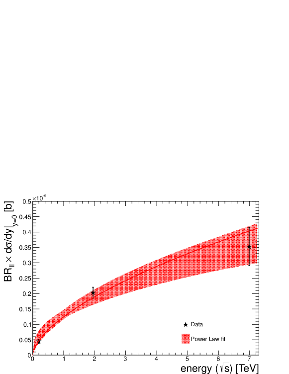
The energy evolution of the inclusive J/ production cross section in proton-proton and proton-antiproton collisions at mid-rapidity is shown in Fig. 1. Here we discuss three approaches to determine the -integrated mid-rapidity cross section at and 5.5 TeV. The first method is a functional form fitting interpolation, while the other two are based on theoretical model predictions, FONLL [17] and LO CEM [20].
3.1 A functional form fitting approach
The cross section energy evolution can be described by a functional form, a power-law distribution:
| (2) |
where , and are free parameters. Although such characterization does not rely on any theoretical basis, it reproduces the measured distribution. The results are depicted in Fig.1 and the interpolation results are reported in Table 2. The uncertainties on the cross section interpolation to and 7 TeV were estimated by re-doing the fit using the upper and lower limits of the PHENIX, CDF and ALICE uncertainties in every possible combination. The envelope of these results defines the uncertainty.
| 2.76 TeV | nb |
|---|---|
| 5.5 TeV | nb |
3.2 FONLL based approach
Another approach consists to use the pQCD energy dependence of charm production cross section at mid-rapidity to describe the inclusive J/ production cross section at mid-rapidity. The B feed-down contribution to the inclusive J/ production cross section is considered via the pQCD beauty production cross section, weighted by the decay branching ratio, BR(), as:
| (3) |
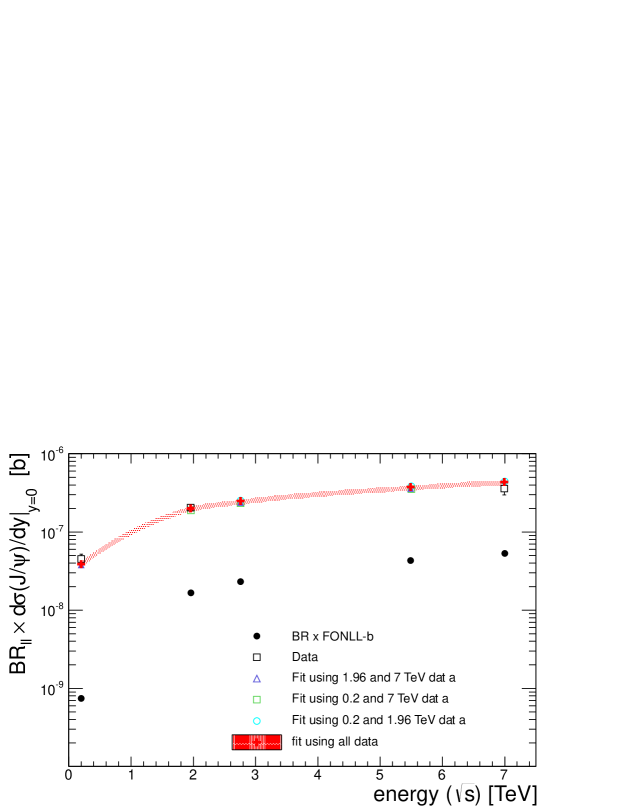
Where is a free parameter, [16] and the charm and beauty differential cross sections are calculated in pQCD at Fixed Order with Next to Leading Log resummation FONLL [17, 18]. The FONLL central predictions were obtained with the CTEQ6.6 [19] parton distribution functions (PDFs). The fit of the variation of J/ inclusive production cross section with the function of Eq. 3, using the FONLL central parameters is shown in Fig. 2.
The FONLL calculation uncertainties were evaluated by varying the PDFs, the quark masses, and the renormalization and factorization scales. These uncertainties are defined by the envelope of the obtained cross section, and are practically described by upper and lower curves. To account for the calculation uncertainties in the interpolation procedure, we refit the distribution considering these upper and lower curves and recalculate the interpolated cross sections. Finally, the interpolation is validated by observing how the results deviate when removing, one by one, the experimental points with the central FONLL parameterization. The results are reported in Table 3.
| Fit | Data | [nb] per [TeV] | ||||
|---|---|---|---|---|---|---|
| FONLL | excluded | 0.2 | 1.96 | 2.76 | 5.5 | 7 |
| central | none | 39 3 | 196 14 | 241 17 | 366 25 | 422 28 |
| lower | none | 45 3 | 201 14 | 229 16 | 299 20 | 332 21 |
| upper | none | 41 3 | 195 14 | 238 17 | 357 24 | 409 27 |
| central | RHIC | 38 3 | 190 15 | 235 19 | 356 28 | 411 31 |
| central | Tevatron | 37 5 | 189 22 | 232 27 | 353 40 | 407 45 |
| central | LHC | 41 3 | 205 16 | 253 19 | 383 28 | 442 32 |
The cross sections evaluated when removing an experimental point to the given energy are in fair agreement (within uncertainties) with the measurements (see Sec. 2). The extrapolated values obtained with the three FONLL curves are compatible, although we note that the fit with the lower FONLL uncertainty band tends to give significantly lower results than the others at high energies 444 This effect is understood as related to the discontinuous shape of the FONLL lower-band uncertainties for direct charm production [17, 18]. , this is a source of systematic uncertainty. We remark that the results of the FONLL interpolation are in good agreement with those of the functional form fit presented in the previous subsection (Sec. 3.1).
3.3 LO CEM based interpolation
The third approach uses the prompt J/ cross section energy dependence as computed in the Colour Evaporation Model (CEM) at Leading Order (LO) [20]. As in the previous subsection (Sec. 3.2), the B-decay contribution is estimated via the FONLL beauty predictions. The fit is defined such that the normalization of the LO CEM calculation is left as a free parameter, :
| (4) |
Different LO PDFs have been considered for this exercise555 It is worth noting that LO CEM based interpolation results using other parton distribution functions are compatible within uncertainties with the ones reported here. . Here, we only report the results obtained with CTEQ6 [21] and MRST01 [22]. The best fit is obtained with the CTEQ6 PDF set and is shown in Fig. 3.
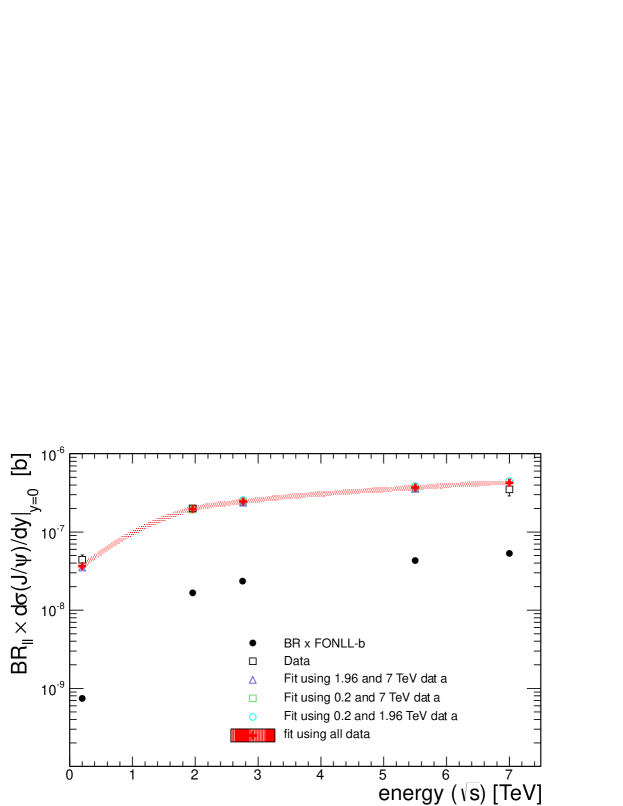
Similarly to the other approaches, the interpolation has been validated by removing the data points one by one from the fit. The results are summarized in Table 4.
| Fit | Data | [nb] per [TeV] | ||||
|---|---|---|---|---|---|---|
| LO CEM | excluded | 0.2 | 1.96 | 2.76 | 5.5 | 7 |
| CTEQ6 | none | 36 3 | 198 14 | 245 17 | 370 25 | 425 29 |
| MRST01 | none | 29 2 | 194 14 | 248 18 | 399 28 | 470 33 |
| CTEQ6 | RHIC | 35 3 | 191 15 | 236 19 | 356 28 | 410 31 |
| CTEQ6 | Tevatron | 36 5 | 193 23 | 239 28 | 362 41 | 416 47 |
| CTEQ6 | LHC | 38 3 | 208 16 | 257 19 | 388 28 | 446 32 |
The CTEQ6 and MRST01 derived calculations are consistent with each other. The cross sections obtained when removing experimental points are also in good agreement (within uncertainties) with the measurements (see Sec. 2). These results also agree with those of the two previous approaches (Sec. 3.1 and Sec. 3.2).
3.4 Results
The values obtained for the inclusive J/ cross sections at and 5.5 TeV, at mid-rapidity, using the functional form, the FONLL and the LO CEM based fits are presented in Table 5, together with the and the number of degrees of freedom of the fit.
| Fit | (ndf) | |
|---|---|---|
| 1.5 (1) | ||
| FONLL central | 1.0 (2) | |
| FONLL upper | 0.57 (2) | |
| FONLL lower | 0.06 (2) | |
| LO CEM CTEQ6 | 1.3 (2) | |
| LO CEM MRST01 | 4.4 (2) | |
| Fit | [nb] | |
| TeV | TeV | |
| FONLL central | ||
| FONLL upper | ||
| FONLL lower | ||
| LO CEM CTEQ6 | ||
| LO CEM MRST01 | ||
| Result for inclusive J/ | ||
| Estimate for prompt J/ | ||
The fit uncertainties at (5.5) TeV are of for the LO CEM and the FONLL fits, while they are of () for the functional form approach666 When dealing with asymmetric uncertainties, we quote as relative error the average between the upper and the lower value of the asymmetric uncertainties. . To combine these results we:
-
1.
discard the LO CEM MRST01 fit, that has a /ndf ,
-
2.
compute the average of the three FONLL values,
-
3.
estimate the weighted average of the power-law fit, the FONLL-average (ii) and the LO CEM CTEQ6 results.
We sort the uncertainties of the combined result in two components. One is related to the spread of the values obtained with the different approaches, resulting in an uncertainty band covering the whole range of values. We will refer to this component of the uncertainty as the model related one. The other component is related to the fit uncertainties and includes the influence of the experimental measurements uncertainties. For this contribution, that we will quote as fit uncertainty, we (conservatively) assume the largest of the relative fit uncertainties (the functional form fit one), that is of 13% (15%) at 2.76 (5.5) TeV. The combined results for the inclusive J/ cross section at mid-rapidity are quoted in Table 5.
Finally, an estimate of the prompt J/ production cross section at mid-rapidity can be reported subtracting the B feed-down contribution. The LHCb results at TeV and indicate that the contribution from B-decays is 10% with a 15% relative uncertainty [8]. CDF [12] measured the B feed-down fraction as a function of for GeV/c. If we consider that for GeV/c it is , we obtain a -integrated B-decay contribution of 10.5%. Assuming that the B-decay contribution to the inclusive J/ production cross section at 2.76 and 5.5 TeV is 10% with a (conservative) uncertainty of 30%, we obtain the prompt J/ cross section at mid-rapidity reported in Table 5.
4 Rapidity distribution
The knowledge of the rapidity dependence of J/ production at 2.76 and 5.5 TeV is crucial in order to provide a reference for the measurements performed at large rapidities. Here we focus on the estimates at (ALICE muon spectrometer) and (region where the CMS acceptance for quarkonia goes down to low ). We consider and compare the interpolation results based on the FONLL and the LO CEM calculations used for the calculation of the mid-rapidity cross section (Sec. 3) with those obtained with a functional form fit approach. For this exercise, we consider the measurements at RHIC [11] and at the LHC [6, 7, 8].
4.1 Interpolation based on theoretical calculations
The FONLL and LO CEM calculations (see Sec. 3.2 and Sec. 3.3) provide predictions for the production cross section rapidity dependence. In order to test their ability to predict the inclusive J/ rapidity shape at different energies, we fit the measured rapidity distributions at GeV and 7 TeV with a model-derived function. The chosen fit function is similar to the form of Eq. 3 and Eq. 4 and is defined as:
| (5) |
We fix the (model dependent) parameters to be those obtained from the mid-rapidity fits 777 Fixing the parameter allows us to fix the relative normalization of the prompt and feed-down contributions at mid-rapidity. in Sec.3 and we let the overall normalization () be the only free parameter of the fit. The fits are shown in Figs. 4 and 5, and their values are summarized in Table 6.
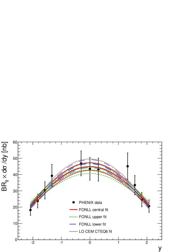
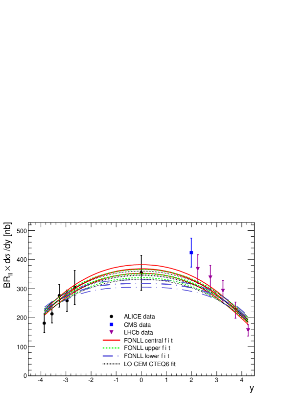
We observe that for all the fits: all the models are compatible with the measured inclusive J/ rapidity distribution at both 200 GeV and 7 TeV. The predictions of these models are expressed here in terms of an extrapolation factor from mid- to forward rapidity, defined as:
| (6) |
The values of for the considered models at the energies and rapidities of interest are reported in Table 6.
| GeV | TeV | |||
| Fit | (ndf) | (ndf) | ||
| FONLL central | 4.1 (10) | 1.100.06 | 10.9 (11) | 0.870.03 |
| FONLL upper | 5.6 (10) | 0.980.05 | 13.6 (11) | 0.850.03 |
| FONLL lower | 3.6 (10) | 0.980.05 | 19.0 (11) | 0.950.04 |
| LO CEM CTEQ6 | 3.1 (10) | 1.290.07 | 15.2 (11) | 0.820.03 |
| Fit | TeV | TeV | ||
| FONLL central | 0.85 | 0.59 | 0.88 | 0.68 |
| FONLL upper | 0.87 | 0.63 | 0.90 | 0.72 |
| FONLL lower | 0.91 | 0.69 | 0.94 | 0.80 |
| LO CEM CTEQ6 | 0.87 | 0.64 | 0.90 | 0.73 |
| Average | ||||
| [nb] | ||||
| TeV | TeV | |||
| 2.0 | ||||
| 3.25 | ||||
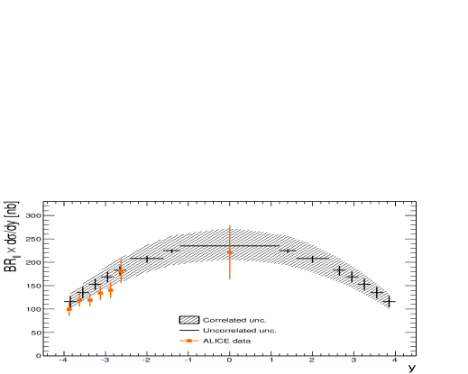
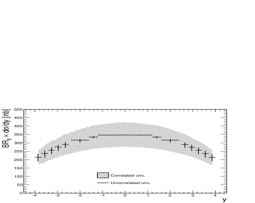
The results are a combination of these values. We first compute the average of the FONLL estimates and then the average between the FONLL-average and the LO CEM CTEQ6 value. The uncertainties are defined by the envelope of all the values. The inclusive forward rapidity cross sections can then be obtained by multiplying the mid-rapidity cross sections of Table 5 by the forward rapidity factors. The uncertainties are split in a correlated (from the mid-rapidity cross section) and an uncorrelated (from the factor) component. The results for the inclusive J/ cross section at forward rapidities are reported on Table 6.
4.2 A functional form fit approach: universal rapidity distribution
In this subsection we explore a model independent approach to the extrapolation of the rapidity distribution, based on the search for an universal energy scaling behaviour in the rapidity distributions measured at different energies. The advantage of this approach is that there is no a priori assumption, and the results only depend on the existing measurements and their uncertainties. To compare the -differential cross sections at 200 GeV and at 7 TeV, these values are renormalized by the -integrated cross section at . We draw the obtained values versus: , and , where is the J/ rapidity, and . The resulting distributions are shown in Fig. 7.
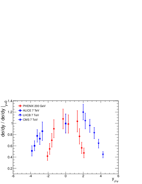
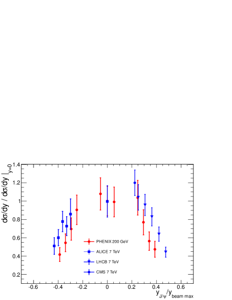
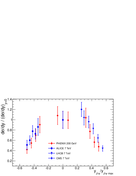
The similarity between the distributions obtained at 200 GeV and 7 TeV is remarkable, the most striking case being the scaling with . We then choose as a scaling variable, and perform global fits to the RHIC and LHC data with suitable functions, the purpose being to define -independent rapidity distribution functions that can be used for the calculations at =2.76 and 5.5 TeV. We note that the values used to normalize the -differential cross sections in Fig. 7, their value at y=0, is not an optimal choice since depends strongly on a single data point. In the following we will re-evaluate this normalization for each functional form.
The first fit function considered is a Gaussian distribution, we consider that:
| (7) |
where is the width of the Gaussian and is a normalization factor obtained via Gaussian fit separately for the two energies. The result of the fit is shown in Fig. 8. For comparison, the RHIC-only and the LHC-only fit results are also drawn, showing that the fit is stable versus excluding data points at a given energy. Also, it is worth noting that uncertainties are reduced when considering all data points together.
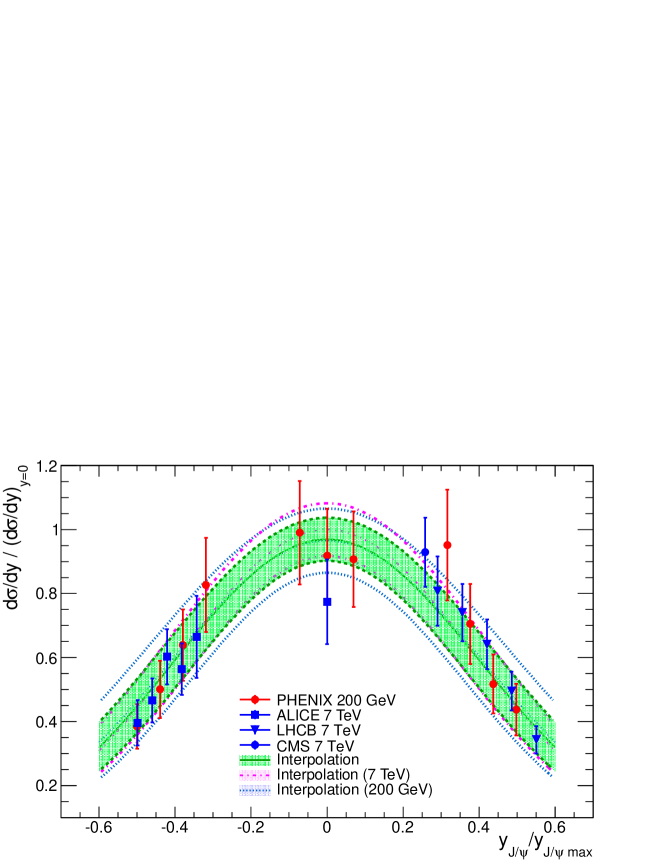
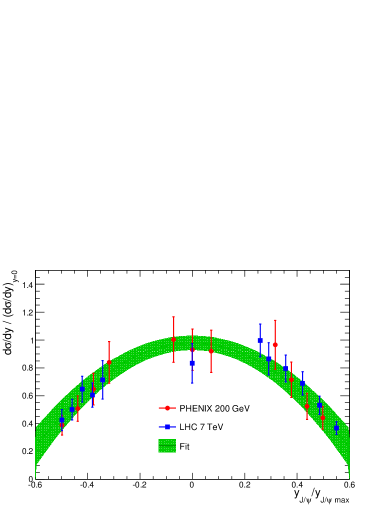
We compare the Gaussian fit results to those from a set of polynomial functions, defined as:
| (8) |
where is an even number (up to ). The resulting fits are shown in Fig. 9. We deduce from the ndf values, reported in Table 7, that all the functions are compatible with the measured -differential distributions. The measurement uncertainties are not small enough to discriminate between quite different rapidity shapes, data driven extrapolations are affected by large uncertainties.
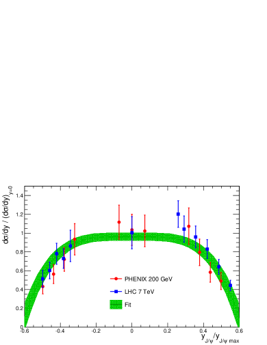
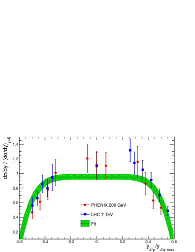
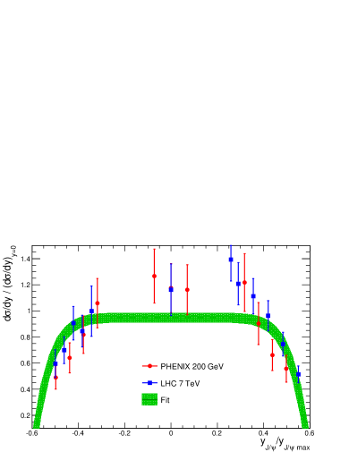
The scaling factor , defined in Eq. 6, has been evaluated for all the considered functional form functions. The results are summarized in Table 7.
| Fit | /ndf | A | B | |
|---|---|---|---|---|
| Gaussian | 11.6/21 | ( | ||
| Poly–(n=2) | 9.2/21 | |||
| Poly–(n=4) | 17.3/21 | |||
| Poly–(n=6) | 27.5/21 | |||
| Poly–(n=8) | 36.3/21 | |||
| Fit | TeV | TeV | ||
| Gaussian | ||||
| Poly–(n=2) | ||||
| Poly–(n=4) | ||||
| Poly–(n=6) | ||||
| Poly–(n=8) | ||||
| Average | ||||
| [nb] | ||||
| TeV | TeV | |||
| 2.0 | ||||
| 3.25 | ||||
Though it is observed that polynomial functions with and exhibit a larger than the ones with or and the Gaussian forms, the experimental measurements do not allow to disregard any fit function. We combine these results by computing their weighted average. The uncertainty is given by the envelope of their uncertainties. The results are reported in Table 7. For completeness, a similar exercise was performed using the beam rapidity scaling () instead of the J/ relative rapidity (). The obtained forward rapidity scaling factors differ by less than 2%. Since the difference is negligible with respect to the other uncertainties, we will neglect it. Using the factors reported here and our estimates of the mid-rapidity cross sections (Table 5), we obtain the inclusive differential cross sections quoted in Table 7. More precise measurements of the J/ rapidity distribution would be needed to disentangle between different fit functions and reduce the interpolation uncertainties.
4.3 Discussion of the rapidity dependence results
We observe that the results obtained with the functional form fits (Sec. 4.2) are in agreement with those obtained by the interpolation based on the FONLL and LO CEM calculations (Sec. 4.1). In all cases, the functional form approach involves larger uncertainties, explained by the fact that it assumes no a priori knowledge of the rapidity shape. Here, we choose not to combine the results obtained with these two approaches.
5 Transverse momentum distributions
In this section we study the inclusive J/ transverse momentum distribution. To compare the existing measurements at different energies and rapidity domains, we normalize their -integrated cross section to unity and plot them together versus the variable, defined as:
| (9) |
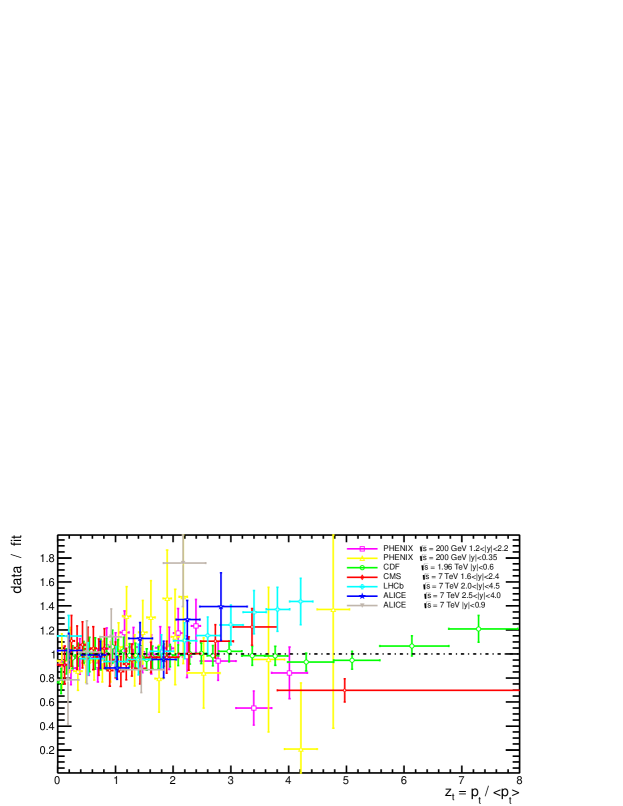
where the values of are given in Table 1. The resulting distributions (see Fig. 10) show a universal behaviour which can be fitted by the following function:
| (10) |
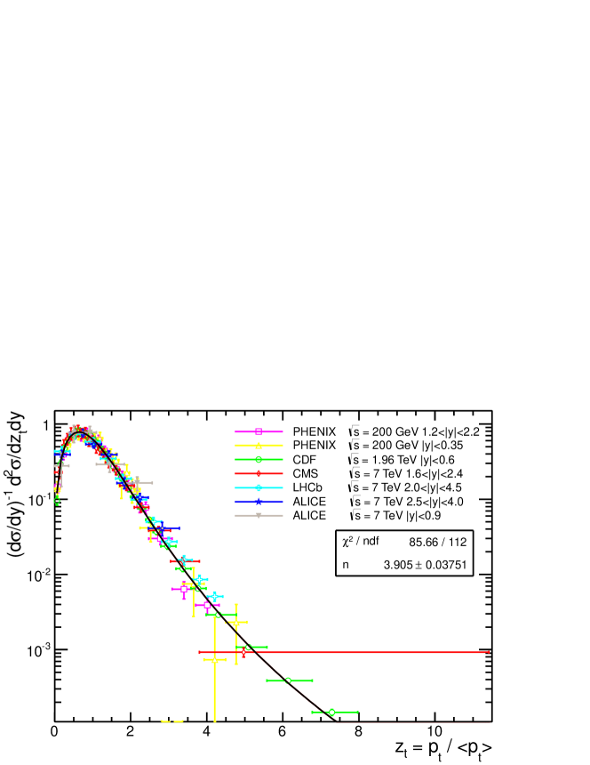
where follows from the normalization to unity. Requiring , meaning that computed by the fit function is equal to that of Table 1, results in: . We are then left with only one free parameter . We do a global fit to all the experimental data and obtain: (see Fig. 10). The systematic uncertainties on the parameter are evaluated by performing three global-like fits excluding one by one the data at 200 GeV, 1.96 TeV and 7 TeV. This gives finally: . To demonstrate the scaling versus variable in more details, we plot in Fig. 11 the ratio of the experimental data to the fit function value at each data point. We have checked that this fit function describes well also the prompt J/ data at 7 TeV [7, 8]. Similar fit of the scaling function Eq. (10) to the meson spectra measured at 1.8 TeV [23] and 7 TeV [24, 25] gives .
| Data excluded | [TeV] | |||||
|---|---|---|---|---|---|---|
| 0.2 | 1.96 | 2.76 | 5.5 | 7 | ||
| none | 2.31 | 2.48 | ||||
| RHIC | 2.52 | 2.51 | 2.50 | |||
| GeV/ | Tevatron | 2.17 | 2.25 | 2.44 | ||
| LHC | 2.67 | 3.01 | 3.15 | |||
| Syst. Unc. | 48% | 13% | 12% | 17% | 25% | |
The next step to obtain the distributions at 2.76 and 5.5 TeV is to estimate the J/ at these two energies. For this we fit the PHENIX, CDF, CMS, ALICE and LHCb data by a power-law function of energy. The results are reported in Table 8. To evaluate the calculation systematics, data points at different energies have been removed one by one. The last row of Table 8 presents the systematic uncertainty on , estimated as the difference between the extrapolated and measured values for = 200 GeV, 1.96 TeV and 7 TeV, and the spread of the results from the global fit and the fits excluding data points for = 2.76 TeV and 5.5 TeV.
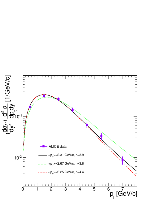
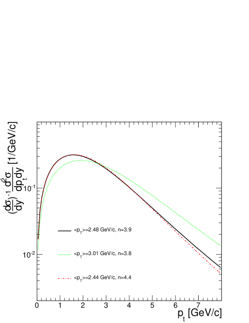
The distribution interpolation at 2.76 and 5.5 TeV is done using Eq. (10) and the corresponding . The resulting central distributions and their uncertainty bands are shown in Fig. 12(a) and Fig. 12(b) respectively.
6 Comparison with the ALICE measurements at TeV
The ALICE collaboration did recently measure the inclusive J/ production at TeV [10]. The inclusive J/ production cross section at mid-rapidity, nb [10], is in good agreement with the interpolation value, nb, see Table 5. The -integrated rapidity distribution, see Fig. 6(a), is well described by our interpolation. The cross section measurements suggest that the mid- to forward-rapidity factor is: , and . Comparing these values to the interpolation results reported in Tables 6–7, we observe that the theory driven (FONLL and LO CEM) and functional form (Gaussian, polynomial-, polynomial-) calculations reproduce the measured trend. However, the polynomial- and polynomial- functional forms tend to overestimate the measured cross sections at forward-rapidities. The ALICE results at TeV [10] seem then to advocate in favor of neglecting the polynomial- and polynomial- functions of the rapidity interpolation approach for future calculations. If we disregard these two functions, the functional form rapidity interpolation factors at TeV would be of and , while at TeV they would be and , to replace those of Table 7. The measured transverse momentum distribution, Fig. 12(a), is well reproduced by our predictions.
7 Conclusions
A procedure to evaluate the energy dependence of the inclusive (and possibly prompt) J/ integrated and differential cross sections in proton proton collisions has been established and used to compute the J/ cross sections at the same centre of mass energy as the one available (per nucleon pair) in Pb–Pb collisions at the LHC (2.76 TeV at present and 5.5 TeV in the near future). The calculation exploits the available experimental measurements in three distinct steps. The first step consists in describing the energy dependence of the mid-rapidity -integrated cross section (Sec. 3). The expectations from functional form (power-law) and model-driven (FONLL and LO CEM) fits have been combined together. The results are summarized in Table 9. The interpolation systematics is of 15% (20%) at 2.76 (5.5) TeV. The second step is the determination of the scaling factors from mid- to forward rapidities (Sec. 4). Two approaches have been discussed, one based on the theoretically (pQCD) predicted rapidity shape, the other being a functional form approach, based on the energy scaling of the distributions. The results with both methods are compatible, although the functional form approach involves larger uncertainties. Higher precision measurements are needed in order to better constrain the rapidity distribution. The third step is the description of the energy evolution of the transverse momentum distribution (Sec. 5), obtained by assuming an universal scaling of the distributions (Eq. 10). The predicted distributions at and 5.5 TeV are drawn in Figs. 12(a) and 12(b). Our predictions of the -integrated and differential cross sections at TeV are in agreement, within interpolation and experimental uncertainties, with the ALICE measurements at the same energy. These comparisons confirm the appropriateness of our interpolation procedure, that can be used to obtain a pp reference for the analysis of both A–A and p–A data at the LHC.
| [nb] | ||
| x TeV | TeV | |
| 0 | ||
| 2.0 | ||
| 3.25 | ||
Acknowledgements
The authors would like to express their gratitude to J. Schukraft for careful reading and valuable suggestions. Our acknowledgement also goes to D. Stocco, for his help on the LO CEM implementation. Part of this work was supported by the ReteQuarkonii Networking of EU I3 Hadron Physics Program. The work of S.G. was supported partially by the CNRS-RFBR PICS project number 4870.
References
- [1] L. Evans and P. Bryant (editors), JINST 3 S08001 (2008).
-
[2]
ALICE collaboration, J. Phys. G 30, 1517 (2004);
ALICE collaboration, J. Phys. G32, 1295 (2006). - [3] S. Abreu et al., J. Phys. G 35, 054001 (2008).
-
[4]
P.Braun-Munzinger, J.Stachel, Phys. Lett. B 490, 196 (2000);
R.L.Thews, M.Schroedter, J.Rafelski, Phys. Rev. C 63, 054905 (2001). - [5] D. d’Enterria, arXiv:nucl-ex/0302016v3 (2003).
- [6] K. Aamodt et al (ALICE Coll.), Phys. Lett. B 704, 442 (2011).
- [7] CMS Collaboration, Eur. Phys. J. C 71, 1575 (2011).
- [8] R. Aaij et al (LHCb Coll.), Eur. Phys. J. C 71, 1645 (2011).
- [9] G. Aad et al (ATLAS Coll.), Nucl. Phys. B 850, 387 (2011).
- [10] B. Abelev et al (ALICE Collaboration), arXiv:1203.3641 (2012).
- [11] A. Adare et al (PHENIX Coll.), Phys. Rev. Lett. 98, 232002 (2007); and data-table.
- [12] D. Acosta et al (CDF Coll.), Phys. Rev. D71, 032001 (2005).
- [13] M.R. Cosentino (STAR Coll.), Proceedings of Quark Matter 2008 International Conference arXiv:0806.0347v1.
- [14] B. Abbott et al. (D0 Coll.), Phys. Rev. Lett. 82, 35 (1999).
- [15] O. Drapier, Thèse d’habilitation, Université C. Bernard - Lyon 1, 1998.
- [16] K. Nakamura et al. (Particle Data Group), J. Phys. G 37, 075021 (2010).
- [17] M.Cacciari, M. Greco, P. Nason, JHEP 9805 (1998) 007.
- [18] M. Cacciari, private communication.
- [19] P. Nadolsky et al., arXiv:0802.0007.
- [20] M. Glück, J. F. Owens, E. Reya, Phys. Rev. D 17-9 (1978) 2324.
- [21] J. Pumplin et al., Journal of High Energy Physics 07 (2002) 012.
- [22] A.D. Martin et al., Phys. Lett. B 531 (2002) 216-224.
- [23] D. Acosta et al. (CDF Coll.), Phys. Rev. Lett. 88, 161802 (2002).
- [24] V. Khachatryan et al. (CMS Coll.), Phys.Rev. D83, 112004 (2011).
- [25] R. Aaij et al. (LHCb Coll.,) LHCb-CONF-2011-016, arXiv:1202.6579 (2012).