Particles and gravitons creation after inflation from a 5D vacuum

Abstract

We use the Bogoliubov formalism to study both, particles and gravitons creation at the reheating epoch, after a phase transition from inflation to a radiation dominated universe. The modes of the inflaton field fluctuations and the scalar fluctuations of the metric at the end of inflation are obtained by using a recently introduced formalism related to the Induced Matter theory of gravity. The interesting result is that the number of created particles is bigger than $10^{90}$ on cosmological scales. Furthermore, the number of gravitons are nearly $10^{-17}$ times smaller than the number of created particles. In both cases, these numbers rapidly increase on cosmological scales.

I Introduction

Inflation has become the standard paradigm for explaining the homogeneity and the isotropy of our observed Universe 1 ; 2 . During this epoch the energy density of the Universe was dominated by some scalar field (the inflaton), with negligible kinetic energy density, such that the corresponding vacuum energy density was the responsible for the exponential growth of the scale factor of the universe. During this phase a small and smooth region of the order of size of the Hubble radius grew so large that it easily encompassed the comoving volume of the entire presently observed Universe. This is the reason for which the observed Universe is so homogeneous and isotropic. Furthermore, it is now clear that structure in the Universe comes primarily from an almost scale-invariant super-horizon curvature perturbation. This perturbation originates presumably from the vacuum fluctuation, during the almost-exponential inflation, of some field with mass much less than the Hubble parameter $H_{0}$. Indeed, any scalar field whose mass is lighter than $H_{0}$ suffered, in a (quasi) de Sitter epoch, with a scale independent quantum fluctuations spectrum3 ; 4 ; 5 ; 5b .

During inflation, particle production can only occur for particles that are light compared to the Hubble scale without classical conformal invariance; gravitons and massless minimally coupled scalars and light fermions are unique in that respect. Particle creation during inflation was studied many years ago in the framework of standard inflationcal ; calb . The process appeared to be straightforward: in models like new inflation and chaotic inflationchao . These models incorporate a second order phase transition to end inflation, the inflaton field would wind up oscillating around the minimum of its potential near the end of inflation. These oscillations would produce a sea of relativistic particles, if one added (by hand) interaction terms between the inflaton and these lighter species. The direct production from vacuum fluctuations during inflation of X-particle was considered inci . Particle creation has been also considered in warm inflationarywi and fresh inflationaryfi scenarios. More recently, particle creation during inflation was considered in a model of brane inflation where two stacks of mobile branes are moving ultra relativistically in a warped throatbi .

After inflation, the universe could have suffered a phase transition from a de Sitter vacuum dominated state to a decelerated radiation dominated stage. At this moment, a great amount of the potential density energy is transferred to radiation energy density due to the decay of the inflaton field produced by its interaction with other boson fieldsrad ; radb ; radc ; radd ; rade . Some years ago Kaiserkaiser demonstrated that particles produced from the parametric resonance effect when $H\neq 0$ is fewer than in the $H\simeq 0$ case, but can still be exponentially greater than when the resonance is neglected altogether.

On the other hand, in a previous workabm we studied the scalar metric fluctuations of a 5D spacetime background metric $({\cal M},g)$, which is Riemann-flat and hence Ricci-flat: $\hat{\cal R}_{AB}=0$. From the mathematical point of view, the Campbell-Magaard theoremcampbell ; campbellb ; campbellc ; campbelld serves as a ladder to go between manifolds whose dimensionality differs by one. This theorem, which is valid in any number of dimensions, implies that every solution of the 4D Einstein equations with arbitrary energy momentum tensor can be embedded, at least locally, in a solution of the 5D Einstein field equations in vacuum. Because of this, the stress-energy may be a 4D manifestation of the embedding geometry. Physically, the background metric there employed describes a 5D extension of an usual de Sitter spacetime. Inflationary cosmology can be recovered from a 5D vacuumnos ; nosb ; nosc . Other version of 5D gravity, which is mathematically similar, is the membrane theory. In this theory gravity propagates freely on the 5D bulk and the interactions of particles are confined to a 4D hypersurface called ”brane”rs ; rsb ; rsc . Both versions of 5D general relativity are in agreement with observations.

In this work we study both, particle and graviton production after a phase transition occurred after inflation. To make it, we shall consider the solutions obtained at the end of inflation from a 5D vacuum on an effective 4D hypersurface described by a de Sitter metric. After it, we shall use the Bogoliubov formalism to calculate the modes solution for the fields after a phase transition to a radiation dominated epoch. The topic here studied is very important, because the case of inflaton decay into further inflatons may be of interest for dark matter searches. Following their production, the inflatons would decouple from the rest of matterkls . If the inflatons were given a tiny mass, then these bosons could serve as a natural candidate for the missing dark matterkaiser .

II Induced Matter and Embeddings

We consider a 5D manifold (${\cal M},g_{ab}$) with a coordinate system $x\equiv\left\{x^{a}\right\}$. We are interested in a 5D theory of gravity on which we define a 5D vacuum, such that the first variation of the action is ${}^{(5)}\delta{\cal I}=^{(5)}\delta{\cal I}_{E}+^{(5)}\delta{\cal I}_{M}$, where

$$^{(5)}\delta{\cal I}=\frac{1}{2}\int d^{5}x\,\sqrt{|g|}\,\delta g^{ab}\,\left\{\frac{\hat{G}_{ab}}{8\pi G}+\hat{T}_{ab}\right\}.$$ (1)

The first term is the variation of the gravitational Einstein action ${}^{(5)}{\cal I}_{E}$ and the second one is the variation of the matter action ${}^{(5)}{\cal I}_{M}$. Here, $G$ is the gravitational constant, $g$ is the determinant of the covariant tensor metric $g_{ab}$ and $\hat{R}$ is the 5D Ricci scalar on the metric. The energy-momentum tensor of matter, $\hat{T}_{ab}$ is defined from the variation of the matter action ${}^{(5)}{\cal I}_{M}$ under a change of the metric, and will be considered as null to describe the 5D apparent vacuum. The Einstein equations on the 5D manifold ${\cal M}$ (we use $c=\hbar=1$ units)

$$\hat{G}^{a}_{\,\,b}=-8\pi G\,\hat{T}^{a}_{\,\,b},$$ (2)

where $\hat{G}^{a}_{b}$ and $\hat{T}^{a}_{b}$ are respectively the Einstein and Energy Momentum tensors on ${\cal M}$. Furthermore, we can define a scalar function $l(x)$, which represents the foliation of the higher-dimensional manifold. We shall consider that the extra coordinate is space-like. Each hypersurface, $\Sigma_{l}$, is considered as a 4D Lorentzian spacetime. We denote $n_{a}$ as the normal vector to the hypersurface $\Sigma_{l}$

$$n_{a}=-\nabla_{a}l_{,}$$ (3)

such that the expression $n_{a}n^{a}=-1$ normalizes $n^{a}$. Now we can define a coordinate system $y\equiv\{y^{a}\}$ on $\Sigma_{l}$. The basis vectors are

$$e^{a}_{\alpha}=\frac{\partial x^{a}}{\partial y^{\alpha}},\qquad n_{a}e^{a}_{\alpha}=0.$$ (4)

These objects can be used to project 5D tensors (for instance, the metric tensor) into 4D ones (which lives on the $\Sigma_{l}$ hypersurface)

$$e^{a}_{\alpha}e^{b}_{\beta}\,g_{ab}=e^{a}_{\alpha}e^{b}_{\beta}\,(h_{ab}+n_{a}n_{b})=h_{\alpha\beta}.$$ (5)

II.1 Einstein tensor on $\Sigma_{l}$

The extrinsic curvature $K_{\alpha\beta}$ of the 4D hypersurface $\Sigma_{l}$ is a symmetric 2-range tensor given by the derivative of the induced metric in the normal direction to $\Sigma_{l}$

$$K_{\alpha\beta}=e^{a}_{\alpha}e^{b}_{\beta}\nabla_{a}n_{b}.$$ (6)

If now we consider an alternative coordinate system on ${\cal M}:\{y^{\alpha},l\}$, such that

$$dx^{a}=e^{a}_{\alpha}\,dy^{\alpha}+l^{a}dl,$$

where the vector tangent to lines with constant $y^{\alpha}$ can be decomposed into the sum of a part tangent to $\Sigma_{l}$, and a part normal to $\Sigma_{l}$

$$l^{a}=N^{\alpha}e^{a}_{\alpha}+n^{a},$$

such that $l^{a}\partial_{a}l=1$. The 4D vector $N^{\alpha}$ is the shift vector, which describes how the $y^{\alpha}$ coordinate system changes as we move from a given $\Sigma_{l}$ hypersurface to another. Finally, the 5D line element $dS^{2}$ can be written as

$$dS^{2}=h_{ab}dx^{a}dx^{b}=h_{\alpha\beta}\left(dy^{\alpha}+N^{\alpha}dl\right)\left(dy^{\beta}+N^{\beta}dl\right)-dl^{2},$$ (7)

which, for a constant foliation $dl=0$, reduces to

$$ds^{2}=h_{\alpha\beta}\,dy^{\alpha}dy^{\beta}.$$ (8)

In this work we are interested in dealing with a 5D Riemann-flat metric, so that the Ricci tensor is null

$$\hat{R}_{ab}=0.$$ (9)

On each $\Sigma_{l}$ hypersurface, the Gauss-Codazzi equations are

$$\hat{R}_{abcd}\,e^{a}_{\alpha}e^{b}_{\beta}e^{c}_{\gamma}e^{d}_{\delta}=R_{\alpha\beta\gamma\delta}-2K_{\alpha[\delta}K_{\gamma]\beta},$$ (10)

$$\hat{R}_{mabc}n^{m}e^{a}_{\alpha}e^{b}_{\beta}e^{c}_{\gamma}=2K_{\alpha[\beta;\gamma]}.$$ (11)

If we use the expression for the 5D Ricci tensor

$$\hat{R}_{ab}=\left(h^{\mu\nu}e^{m}_{\mu}e^{n}_{\nu}-n^{m}n^{n}\right)\hat{R}_{ambn},$$ (12)

we obtain the contractions of (9)

$$\hat{R}_{ab}e^{a}_{\alpha}e^{b}_{\beta}=0,$$

$$\hat{R}_{ab}e^{a}_{\alpha}n^{b}=0,$$

$$\hat{R}_{ab}n^{a}n^{b}=0.$$ (13)

Using (12) into (13), and making use of (11), we obtain the expressions

$$R_{\alpha\beta}=E_{\alpha\beta}+K_{\alpha}^{\mu}\left(K_{\beta\mu}-K\,h_{\beta\mu}\right),$$ (14)

$$\left(P^{\alpha\beta}\right)_{;\alpha}=\left(K^{\alpha\beta}-h^{\alpha\beta}K\right)_{;\alpha}=0,$$ (15)

$$E_{\mu\nu}h^{\mu\nu}=0,$$ (16)

where $K=h^{\alpha\beta}K_{\alpha\beta}$, $E_{\alpha\beta}=E_{\beta\alpha}$ and $E_{\alpha\beta}=\hat{R}_{manb}n^{m}e^{a}_{\alpha}n^{n}e^{b}_{\beta}$. Notice that the equation (15) means that the second rank (symmetric) tensor $P^{\alpha\beta}$ is conserved on the 4D hypersurface $\Sigma_{l}$. It is important to notice that the Ricci tensor on $\Sigma_{l}$, related to the 5D Riemann flat metric $\hat{R}_{mnlo}=0$, is given by

$$R_{\alpha\beta}=K_{\alpha}^{\mu}\left(K_{\beta\mu}-K\,h_{\beta\mu}\right).$$ (17)

Finally, the Einstein tensor $G^{\alpha\beta}=R^{\alpha\beta}-g^{\alpha\beta}\,R/2$ on a given $\Sigma_{l}$, is

$$G^{\alpha\beta}=E^{\alpha\beta}+K^{\alpha}_{\mu}P^{\mu\beta}-\frac{1}{2}h^{\alpha\beta}K^{\mu\nu}P_{\mu\nu}.$$ (18)

Notice that for a 4D metric induced from a 5D Riemann-flat metric, the Einstein tensor only depends on the extrinsic curvature

$$G^{\alpha\beta}=K^{\alpha}_{\mu}P^{\mu\beta}-\frac{1}{2}h^{\alpha\beta}K^{\mu\nu}P_{\mu\nu}.$$ (19)

II.2 Einstein equations on $\Sigma_{l}$

In this work, we are interested in describing the primordial universe on a 4D hypersurface $\Sigma_{l}$. In order to make it, we shall consider a massless single scalar field $\varphi(x^{a})$, which, we shall consider to describe the physical vacuum on the 5D manifold ${\cal M}$. The kinetic Lagrangian corresponding to this field is

$${\cal L}_{\varphi}=\frac{1}{2}\sqrt{\left|\frac{g}{g_{0}}\right|}\,g^{ab}\varphi_{,a}\varphi_{,b},$$ (20)

where $g=l^{8}\exp{6(N-4\psi)}$ is the determinant of the covariant metric tensor and $g_{0}$ is a dimensional constant. Hence, to describe the energy momentum tensor related to $\varphi$, on ${\cal M}$, we set

$$-8\pi G\,\hat{T}^{ab}=\frac{\partial{\cal L}_{\varphi}}{\partial g_{ab}}-\frac{\partial}{\partial x^{m}}\left[\frac{\partial{\cal L}_{\varphi}}{\partial\left(g_{ab,m}\right)}\right].$$ (21)

It is easy to demonstrate that the $\hat{T}^{ab}$ projected on the hypersurface $\Sigma_{l}$ is

$$T^{\alpha\beta}=\hat{T}^{ab}e^{\alpha}_{a}e^{\beta}_{b}.$$ (22)

Finally, using (22) and (19), we obtain the Einstein equations on $\Sigma_{l}$ obtained from a Riemann-flat 5D vacuum

$$\left.G^{\alpha\beta}\right|_{l}=\left.K^{\alpha}_{\mu}P^{\mu\beta}-\frac{1}{2}h^{\alpha\beta}K^{\mu\nu}P_{\mu\nu}\right|_{l}=e^{\alpha}_{a}e^{\beta}_{b}\left.\,\left\{\frac{\partial{\cal L}_{\varphi}}{\partial g_{ab}}-\frac{\partial}{\partial x^{m}}\left[\frac{\partial{\cal L}_{\varphi}}{\partial\left(g_{ab,m}\right)}\right]\right\}\right|_{l},$$ (23)

that describes the equations of motion for the fields on hypersurfaces with constant $l$ (i.e., for constant foliations). Notice that the equations of motion obtained from a Ricci-flat 5D metric must include the Einstein tensor (18), rather than (19), in the left side of the Einstein equations (23).

III Revisiting the formalism for scalar metric fluctuations on a 5D Riemann-flat metric

We consider the Riemann-flat background metriclebe

$$dS^{2}_{b}=l^{2}dN^{2}-l^{2}e^{2N}dr^{2}-dl^{2},$$ (24)

where $dr^{2}=\delta_{ij}dx^{i}dx^{j}$. Here, $x^{i}$ are the 3D cartesian space-like dimensionless coordinates, $N$ is a dimensionless time-like coordinate and $l$ is the space-like non-compact extra coordinate, which has length units. The non-perturbative metric fluctuations of the background metric (24), are introduced in our analysis by the line element introduced inabm

$$dS^{2}=l^{2}e^{2\psi}dN^{2}-l^{2}e^{2(N-\psi)}dr^{2}-dl^{2},$$ (25)

where the metric function $\psi(N,\vec{r},l)$ describes the gauge-invariant metric fluctuations with respect to the background metric. In order to describe a 5D physical vacuum, we shall consider a massless and free test scalar field $\varphi=\varphi(x^{\alpha},l)$ defined on (25). The dynamics of $\varphi$ can be derived from the action

$${\cal I}={\int}d^{4}x\ dl\sqrt{\left|\frac{g}{g_{0}}\right|}\left(\frac{\hat{R}}{16\pi G}+\frac{1}{2}g^{ab}\varphi_{,a}\varphi_{,b}\right).$$ (26)

Now we consider a semiclassical approximation for the 5D scalar field $\varphi$ in the form $\varphi(N,\vec{r},l)=\varphi_{b}(N,l)+\delta\varphi(N,\vec{r},l)$, with $\varphi_{b}$ denoting the background part of $\varphi$ and $\delta\varphi$ denoting the quantum fluctuations of $\varphi$, which will be considered as very small. This is consistent with a linear approximation for the scalar metric fluctuations. Thus, a first-order approximation in the gauge scalar fluctuations of the form $e^{\pm 2\psi}\simeq 1\pm 2\psi$, will be sufficient in order to have a good description of these fluctuations during inflation, in the present formalism. After making this approximation, one find that the dynamics on 5D of $\varphi_{b}(N,l)$ and $\delta\varphi(N,\vec{r},l)$, are

$$\frac{\partial^{2}\varphi_{b}}{\partial N^{2}} + 3\frac{\partial\varphi_{b}}{\partial N}-\left[l^{2}\frac{\partial^{2}\varphi_{b}}{\partial l^{2}}+4l\frac{\partial\varphi_{b}}{\partial l}\right]=0,$$ (27)

$$\frac{\partial^{2}\delta\varphi}{\partial N^{2}} + 3\frac{\partial\delta\varphi}{\partial N}-e^{-2N}\nabla_{r}^{2}\delta\varphi-\left[l^{2}\frac{\partial^{2}\delta\varphi}{\partial l^{2}}+4l\frac{\partial\delta\varphi}{\partial l}\right]$$ (28)

$$- 2\psi\left[l^{2}\frac{\partial^{2}\varphi_{b}}{\partial l^{2}}+4l\frac{\partial\varphi_{b}}{\partial l}\right]=0.$$

The expression (27) gives the dynamics on the background of $\varphi(N,\vec{r},l)$, whereas Eq. (28) describes the dynamics for the quantum fluctuations $\delta\varphi(N,\vec{r},l)$ in terms of the scalar metric fluctuations $\psi$ and the background field $\varphi_{b}$. On the other hand, the expression for the energy momentum tensor components on the background is

$$-8\pi G\,\hat{T}_{ab}=\left.\frac{\partial{\cal L}_{\varphi}}{\partial g^{ab}}-\frac{\partial}{\partial x^{m}}\left[\frac{\partial{\cal L}_{\varphi}}{\partial\left(g^{ab}_{\,\,\,\,,m}\right)}\right]\right|_{g_{ab}=\bar{g}_{ab},\varphi=\varphi_{b}},$$ (29)

where the Lagrangian density corresponding to the inflaton field is

$${\cal L}_{\varphi}=\frac{1}{2}\sqrt{\left|\frac{g}{g_{0}}\right|}\,g^{ab}\varphi_{,a}\varphi_{,b}.$$ (30)

One can find the linearized equation which describes the dynamics of the salar metric fluctuations $\psi$ on the linearized fluctuating metric $dS^{2}=(1+2\psi)l^{2}dN^{2}-l^{2}e^{2N}(1-2\psi)dr^{2}-d\psi^{2}$abm :

$$\frac{\partial^{2}\psi}{\partial N^{2}} + 7\frac{\partial\psi}{\partial N}+6\psi-e^{-2N}\nabla_{r}^{2}\psi-\frac{2}{3}\left[14l\frac{\partial\psi}{\partial l}+4l^{2}\frac{\partial^{2}\psi}{\partial l^{2}}\right]$$ (31)

$$= -\frac{8\pi G}{3}\left[\frac{\partial\varphi_{b}}{\partial N}\frac{\partial\delta\varphi}{\partial N}+\psi l^{2}\left(\frac{\partial\varphi_{b}}{\partial l}\right)^{2}+l^{2}\frac{\partial\varphi_{b}}{\partial l}\frac{\partial\delta\varphi}{\partial l}\right],$$

where $\psi$ complies with the linearized non-diagonal Einstein equations

$$\frac{\partial^{2}\psi}{\partial x^{i}\partial N}+\frac{\partial\psi}{\partial x^{i}}=4\pi G\frac{\partial\varphi_{b}}{\partial N}\frac{\partial\delta\varphi}{\partial x^{i}},$$ (34)

$$\frac{\partial^{2}\psi}{\partial l\partial N}+2\frac{\partial\psi}{\partial l}=\frac{8\pi G}{3}\left(\frac{\partial\delta\varphi}{\partial N}\frac{\partial\varphi_{b}}{\partial l}+\frac{\partial\varphi_{b}}{\partial N}\frac{\partial\delta\varphi}{\partial l}\right),$$

$$\frac{\partial^{2}\psi}{\partial x^{i}\partial l}=8\pi G\left(\frac{\partial\varphi_{b}}{\partial x^{i}}\frac{\partial\delta\varphi}{\partial l}+\frac{\partial\delta\varphi}{\partial x^{i}}\frac{\partial\varphi_{b}}{\partial l}\right).$$

These equations provide us with the dynamics for both, the scalar field and the 5D gauge-invariant metric fluctuationsabm .

IV Dynamics of fields at the end of inflation on an effective 4D de Sitter background

We consider the background metric (24). If we take a static foliation $l=l_{0}=1/H_{0}$, with the transformations

$$N=t/l_{0}=H_{0}t,$$ (35)

$$R=l_{0}r=1/H_{0}r,$$ (36)

we obtain the effective 4D de Sitter background metric

$$dS^{2}=dt^{2}-e^{2H_{0}t}dR^{2}.$$ (37)

Here, $H_{0}$ is a constant that represents the Hubble parameter. For the relativistic point of view, this means that now we shall move with penta-velocities

$$u^{t}=1,\qquad u^{i}=u^{l}=0.$$ (38)

The effective 4D action on $\Sigma_{H}$ derived from the 5D action (26), reads

$$^{(4)}{\cal I}_{eff}=\int d^{4}x\,\sqrt{\left|\frac{{}^{(4)}g}{{}^{(4)}g_{0}}\right|}\left(\frac{{}^{(4)}R}{16\pi G}+\frac{1}{2}g^{\mu\nu}\Phi_{,\mu}\Phi_{,\nu}+V\right),$$ (39)

where $\Phi(t,\vec{r})\equiv\varphi(t,\vec{r},l)|_{l=H_{0}^{-1}}$ is the massive scalar field induced on $\Sigma_{H}$. Furthermore, ${}^{(4)}g$ is the determinant of the 4D induced metric, which in the case of background metric (37) yields ${}^{(4)}\bar{g}=\exp(6H_{0}t)$. Moreover, in the case of the perturbed metric (25) gives ${}^{(4)}g=\exp[2(3H_{0}t-2\Psi)]$, and ${}^{(4)}g_{0}$ is a dimensionless constant. The induced 4D effective potential $V$ in the action (39), has the form

$$V=-\left.\frac{1}{2}g^{ll}\left(\frac{\partial\varphi}{\partial l}\right)^{2}\right|_{N=H_{0}t,R=r/H_{0},l=l_{0}=1/H_{0}}\,.$$ (40)

Given the quantum nature of the fields $\Phi$ and $\Psi$ it seems convenient to use the quantization procedure. To do it, we impose the commutation relations

$$\left[\Phi(t,\vec{R}),\Pi^{0}_{(\Phi)}(t,\vec{R}^{\prime})\right]=i\,\delta^{(3)}\left(\vec{R}-\vec{R}^{\prime}\right),\quad\left[\Psi(t,\vec{R}),\Pi^{0}_{(\Psi)}(t,\vec{R}^{\prime})\right]=i\,\delta^{(3)}\left(\vec{R}-\vec{R}^{\prime}\right),$$ (41)

where $\Pi^{0}_{(\Psi)}$ and $\Pi^{0}_{(\Phi)}$ are the canonical momentums for $\Phi$ and $\Psi$, respectively. We can derive the commutation relations on the effective 4D background metric. If the inflaton and metric fluctuations are small, these commutators can be approximated to

$$\left[\Phi(t,\vec{R}),\dot{\Phi}(t,\vec{R}^{\prime})\right]\simeq i\sqrt{\left|\frac{{}^{(4)}g_{0}}{{}^{(4)}\bar{g}}\right|}\delta^{(3)}\left(\vec{R}-\vec{R}^{\prime}\right),$$ (42)

$$\left[\Psi(t,\vec{R}),\dot{\Psi}(t,\vec{R}^{\prime})\right]\simeq i\frac{4}{9}\pi G\sqrt{\left|\frac{{}^{(4)}g_{0}}{{}^{(4)}\bar{g}}\right|}\delta^{(3)}\left(\vec{R}-\vec{R}^{\prime}\right).$$ (43)

In this section we shall examine the evolution of the background inflaton field, jointly with the metric and inflaton fluctuations.

IV.1 Dynamics of the background field at the end of inflation

The dynamics of the background inflaton dynamics on the effective 4D background (de Sitter) metric is described by the equation (27) with $l=l_{0}=1/H$ and $N=H_{0}\,t$. In what follows we shall define $\Phi_{b}(t)=\varphi_{b}(N=H_{0}t,l=l_{0}=1/H_{0})$. After making separation of variables in (27), we obtain

$$\frac{\partial^{2}\Phi_{b}}{\partial t^{2}}+3H_{0}\frac{\partial\Phi_{b}}{\partial t}+H_{0}^{2}m^{2}\Phi_{b}=0,$$ (44)

$m$ being a dimensionless separation constant. The background Friedmann equation $G^{t}_{\,\,t}=-8\pi G\left<T^{t}_{\,\,t}\right>$, on the effective 4D hypersurface is

$$\left.\left(\frac{\partial\varphi_{b}}{\partial t}\right)^{2}+H_{0}^{2}\left(l\frac{\partial\varphi_{b}}{\partial l}\right)^{2}\right|_{l=H_{0}^{-1}}=\left.\frac{3}{4\pi G}\frac{1}{l^{2}}\right|_{l=H_{0}^{-1}}=\frac{3H_{0}^{2}}{4\pi G}.$$ (45)

The complete solution for eqs. (44) and (45) is with $m=0$, such that the inflaton field is a constant of time: $\Phi_{b}=\sqrt{\frac{1}{12\pi G}}$abm .

However, at the end of inflation the second term in the equation (44) can be neglected and that equation can be approximated to

$$\frac{\partial^{2}\Phi_{b}}{\partial t^{2}}+H_{0}^{2}m^{2}\Phi_{b}\approx 0.$$ (46)

In what follows we shall consider the dynamics of the inflaton field governed by the approximated equation (46) with the effective 4D Friedman equation (45). We shall consider that at the end of inflation the mass of the inflaton field is of the order of the Hubble parameter. In particular, if we consider $m=2$, the dynamics of the metric fluctuations described by (31) is simplified and we obtain the following solution for (46)

$$\Phi_{b}(t)=\Phi_{0}\cos(2H_{0}t+\delta),$$ (47)

where $\Phi_{0}=\frac{1}{4}\sqrt{\frac{3}{\pi G}}$ and $\delta$ is some constant of integration to be determined.

IV.2 Dynamics of metric fluctuations at the end of inflation

Using the result (47), and combining equations (31) to (34) over the 4D hypersurfaces $\Sigma_{H}:l=l_{0}=H_{0}^{-1}$, we obtain an uncoupled equation for $\Psi(t,\vec{r})$

$$\frac{\partial^{2}\Psi}{\partial t^{2}}+3H_{0}\frac{\partial\Psi}{\partial t}+2H_{0}^{2}\Psi\left(1-3\cos^{2}(2H_{0}t+\delta)+S^{2}\tan(2H_{0}t+\delta)\right)-3H_{0}^{2}e^{-2H_{0}t}\nabla_{r}^{2}\Psi=0,$$ (48)

where $S^{2}=4k^{2}_{l}$, $k_{l}$ being a separation constant.

Following a canonical quantization process, the field $\Psi$ can be expanded in Fourier modes

$$\Psi(t,\vec{R})=\frac{1}{(2\pi)^{3/2}}\int d^{3}k\left[a_{k}\,e^{i\vec{k}\cdot\vec{R}}\xi_{k}(t)+a_{k}^{\dagger}\,e^{-i\vec{k}\cdot\vec{R}}\xi_{k}^{*}(t)\right],$$ (49)

where the annihilation and creation operators $a_{k}$ and $a_{k}^{\dagger}$, satisfy the usual commutation algebra

$$[a_{k},a_{k^{\prime}}^{\dagger}]=\delta^{(3)}(\vec{k}-\vec{k^{\prime}}),\quad[a_{k},a_{k^{\prime}}]=[a_{k}^{\dagger},a_{k^{\prime}}^{\dagger}]=0.$$ (50)

Using the commutation relation (50) and the Fourier expansion (49), we obtain the normalization condition for the modes $\xi_{k}(t)$

$$\xi_{k}(t)\dot{\xi}^{*}_{k}(t)-\xi^{*}_{k}(t)\dot{\xi}_{k}(t)=i\frac{4\pi G}{9}\left(\frac{a_{0}}{a}\right)^{3}H_{0}^{3},$$ (51)

where $a(t)=e^{H_{0}t}$ is the scale factor in the 4D metric and $a_{0}=e^{H_{0}t_{0}}$, being $t_{0}$ the cosmic time at the end of inflation. Inserting (49) in (48), we obtain that the modes $\xi_{k}(t)$ satisfy

$$\frac{\partial^{2}\xi_{k}}{\partial t^{2}}+3H_{0}\frac{\partial\xi_{k}}{\partial t}+2H_{0}^{2}\xi_{k}\left(1-3\cos^{2}(2H_{0}t+\delta)+\frac{3}{2}k^{2}e^{-2H_{0}t}+S^{2}\tan(2H_{0}t+\delta)\right)=0.$$ (52)

Lets us consider the phase $\delta$ so that at the end of inflation $2H_{0}t+\delta\approx\pi$. In this case, the equation (52) leads to

$$\frac{\partial^{2}\xi_{k}}{\partial t^{2}}+3H_{0}\frac{\partial\xi_{k}}{\partial t}+2H_{0}^{2}\xi_{k}\left(\frac{3}{2}k^{2}e^{-2H_{0}t}-2\right)=0.$$ (53)

By means of the equation (51) and choosing the Bunch-Davies vacuum condition, the normalized solution of (53), is

$$\xi_{k}(t)=\frac{\pi H_{0}}{3}\sqrt{G}\left(\frac{a_{0}}{a}\right)^{3/2}{\cal H}^{(2)}_{\nu}[x(t)],$$ (54)

where ${\cal H}^{(2)}_{\nu}[x(t)]$ is the second kind Hankel function, $\nu=5/2$ and $x(t)=\sqrt{3}\>k\>e^{-H_{0}t}$.

IV.3 Dynamics of the inflaton field fluctuations at the end of inflation

Now, employing again the equations (31) to (34) over the 4D hypersurfaces $\Sigma_{H}:l=l_{0}=H_{0}^{-1}$ and incorporating the solution (47), we obtain that the 4D quantum fluctuations for the inflaton field are determined by the equationabm

$$\frac{\partial^{2}\delta\Phi}{\partial t^{2}}+3H_{0}\frac{\partial\delta\Phi}{\partial t}-H_{0}^{2}e^{-2H_{0}t}\nabla_{r}^{2}\delta\Phi-H_{0}^{2}\left.\left[l^{2}\frac{\partial^{2}\delta\varphi}{\partial l^{2}}+4l\frac{\partial\delta\varphi}{\partial l}\right]\right|_{l=H_{0}^{-1}}+8H_{0}^{2}\Psi\Phi_{b}=0,$$ (55)

Performing a Fourier expansion of $\delta\Phi$ in the form

$$\delta\Phi(t,\vec{R})=\frac{1}{(2\pi)^{3/2}}{\int}d^{3}K\left[a_{K}e^{i\vec{K}\cdot\vec{R}}\eta_{K}(t)+a^{\dagger}_{K}e^{-i\vec{K}\cdot\vec{R}}\eta^{*}_{K}(t)\right],$$ (56)

where the annihilation and creation operators $a_{K}$ and $a_{K}^{\dagger}$ satisfy the commutation algebra given by (50). Inserting (55) and (49) in (54), it leads to

$$\frac{\partial^{2}\eta_{K}}{\partial t^{2}}+3H_{0}\frac{\partial\eta_{K}}{\partial N}+H_{0}^{2}K^{2}e^{-2H_{0}t}-H_{0}^{2}\left.\left[l^{2}\frac{\partial^{2}\eta_{K}}{\partial l^{2}}+4l\frac{\partial\eta_{K}}{\partial l}\right]\right|_{l=H_{0}^{-1}}+8H_{0}^{2}\xi_{K}\Phi_{b}=0.$$ (57)

The previous equation is inhomogeneous, non separable and presents a source term. The general solution will be the solution of the homogeneous equation plus a particular solution

$$\eta_{K}(t)=\left[f(t)\cos{(k\sqrt{3}e^{-H_{0}t})}+g(t)\sin{(k\sqrt{3}e^{-H_{0}t})}\right]+\frac{e^{3H_{0}(t_{0}-t)}}{2}\sqrt{\frac{\pi}{H_{0}}}\>{\cal H}^{(2)}_{\mu}\left[x(t)\right],$$ (58)

where $f(t)$ and $g(t)$ are polinomial functions of $e^{\frac{H_{0}t}{2}}$, and ${\cal H}^{(2)}_{\mu}\left[x(t)\right]$ is the second kind Hankel function with $\mu=\frac{\sqrt{9-4M^{2}}}{2}$ and $x(t)=ke^{-H_{0}t}$. Here, we have used both, the Bunch - Davies vacuum and the normalization conditions

$$\dot{\eta_{h}}_{K}^{*}{\eta_{h}}_{K}-\dot{\eta_{h}}_{K}{\eta_{h}}_{K}^{*}=i\left(\frac{a_{0}}{a}\right)^{3},$$ (59)

for the Fourier modes of the homogeneous solution.

Towards the end of inflation one can neglect the lower terms of $f(t)$ and $g(t)$, to take only those with higher order in $e^{\frac{H_{0}t}{2}}$. The term with the Hankel function can be neglected too, so that we obtain

$$f(t)=ig(t)=\frac{40H_{0}}{3\mu(25-4\mu^{2})}\sqrt{\frac{\sqrt{3}}{2K^{5}}}\>e^{\frac{3}{2}H_{0}t_{0}}\>e^{\frac{5}{2}H_{0}t}.$$ (60)

Finally, the approximated solution for the modes of the inflaton field fluctuations at the end of inflation can be rewritten as

$$\eta_{K}(t)=f(t)e^{-ik\sqrt{3}\>e^{-H_{0}t}},$$ (61)

where $f(t)$ is given by (60).

V Particle Creation after a phase transition, after inflation

To consider the particle creation lets first rewrite the solution (61) in terms of the conformal time in a spatially flat 4D Friedmann-Robertson-Walker cosmology $d\tau\equiv a^{-1}dt=e^{-H_{0}t}dt$. Furthermore, we obtain that the modes of the inflaton fluctuations are

$$\eta_{K}(\tau)=f(\tau)e^{ik\sqrt{3}\>H_{0}a_{0}\tau},$$ (62)

and their derivatives with respect to $\tau$, which we denote with a prime, are

$$\eta^{\prime}_{K}(\tau)=f(\tau)e^{ik\sqrt{3}\>H_{0}a_{0}\tau}\left(iK\sqrt{3}H_{0}a_{0}-\frac{5}{2\tau}\right),$$ (63)

where

$$f(\tau)=\frac{40\>H_{0}\>e^{\frac{3}{2}H_{0}t_{0}}}{3\mu(25-4\mu^{2})}\sqrt{\frac{\sqrt{3}}{2K^{5}}}\>(-H_{0}a_{0}\tau)^{-\frac{5}{2}}.$$ (64)

In order to calculate the number of particles produced for each mode ($N_{k}$), we match the solutions obtained at the end of inflation, with those of the long-wavelength modes during a phase transition from inflation to the radiation-dominated era. To calculate this last solutions, we make use of the Bogolyubov transformation (6 ). For the long-wavelength modes we can approximate the phase transition to be instantaneous, occurring at some time $\tau_{0}$. So, we have that

$$\begin{array}[]{ccl}$for$&\>\>\>\tau<\tau_{0}:&\>\>\>a(\tau)=-\frac{1}{H\tau},\\ $for$&\>\>\>\tau>\tau_{0}:&\>\>\>a(\tau)=-a_{0}(\tau-\widetilde{\tau}),\end{array}$$ (65)

where $\widetilde{\tau}=\tau_{0}-(H^{2}\tau_{0})^{-1}$. For convenience, we set $a(\tau_{0})=a_{0}$, so we obtain that $\tilde{\tau}=0$, $H_{0}=a_{0}^{-1}$ and $\tau_{0}=-1$. After the transition, the Hubble parameter is no longer constant, $H\equiv H(\tau)$, and we get:

$$\begin{array}[]{ccl}$for$&\>\>\>\tau<\tau_{0}:&\>\>\>H(\tau)=H_{0},\\ $for$&\>\>\>\tau>\tau_{0}:&\>\>\>H(\tau)=\frac{H_{0}}{\tau^{2}}.\end{array}$$ (66)

In what follows we shall compute the number of particles and gravitons in the radiation dominated era, which takes place after a phase transition from the inflationary epoch.

V.1 Particle creation from inflaton field fluctuations in the radiation dominated era

In order to calculated the number of created particles after a phase transition, we calculate the modes of the inflaton field fluctuations taking into account the Bogolyubov transformations

$$\eta_{K}(\tau>\tau_{0})=\frac{H_{0}\tau}{\sqrt{2\sqrt{3}\>K}}\left[\alpha_{K}e^{-iK\sqrt{3}\>\tau^{-1}}+\beta_{K}e^{iK\sqrt{3}\>\tau^{-1}}\right],$$ (67)

so that their temporal derivatives are

$$\eta^{\prime}_{K}(\tau>\tau_{0})=\frac{H_{0}}{\sqrt{2\sqrt{3}\>K}}\left[\alpha_{K}e^{-iK\sqrt{3}\>\tau^{-1}}\left(1+\frac{i\sqrt{3}K}{\tau}\right)+\beta_{K}e^{iK\sqrt{3}\>\tau^{-1}}\left(1-\frac{i\sqrt{3}K}{\tau}\right)\right].$$ (68)

To calculate the coefficients $\alpha_{K}$ and $\beta_{K}$, we use the continuity of $\eta_{K}$ and $\eta^{\prime}_{K}$ at $\tau=\tau_{0}=-1$, so that

$$\beta_{K}=a_{0}\,f(\tau_{0})\,\sqrt{2K\sqrt{3}}\left(1-\frac{7i}{2K\sqrt{3}}\right),$$ (69)

$$\alpha_{K}=2\,a_{0}\,f(\tau_{0})\,\sqrt{2K\sqrt{3}}\left(\frac{7i}{2K\sqrt{3}}-1\right)e^{-2iK\sqrt{3}},$$ (70)

where

$$f(\tau_{0})=\frac{40\>H_{0}\>e^{\frac{3}{2}H_{0}t_{0}}}{3\mu(25-4\mu^{2})}\sqrt{\frac{\sqrt{3}}{2K^{5}}}.$$ (71)

Finally, by using $N_{K}=\left|\beta_{K}\right|^{2}$ we obtain the number of created particles with a wavenumber $K$

$$N_{K}=2\,a_{0}^{2}\left|f(\tau_{0})\,\right|^{2}K\sqrt{3}\left(1+\frac{29}{12K^{2}}\right).$$ (72)

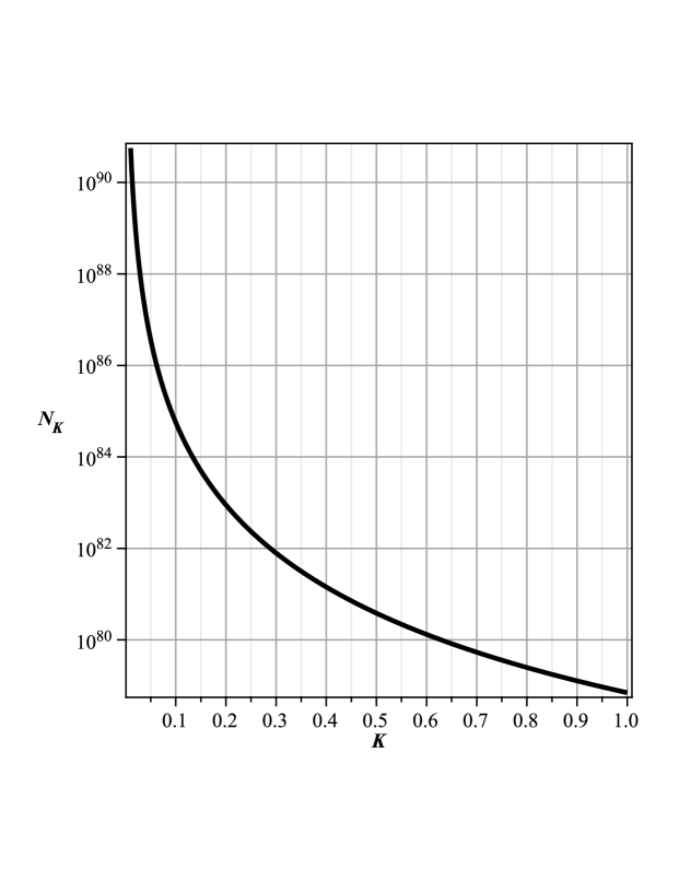
To estimate numerically the number of particles created after the phase transition on cosmological scales (small wavenumbers), we shall consider that the number of e-folds, $N_{e}$, at the end of inflation is at least: $N_{e}>H_{0}t_{0}\sim 60$. The value of $K$ depends upon the details of the transition between inflation and the radiation dominated epoch. For long-wavelength modes (on cosmological super Hubble scales), the transition can be considered as abrupt. In general one expects that $K<1$vi . For instance, if we take $0.01<K<1$ and $H_{0}\sim 6\times 10^{-6}\>M_{p}$, with $\mu(25-4\mu^{2})\simeq 24$, we obtain

$$5.5\times 10^{78}<N_{K}<5.64\times 10^{90},$$ (73)

which, in cases where the wavenumber is small, is a number sufficiently important to agree with the desired values for entropy ${\cal S}>10^{89}$.

In the figure (1) was plotted the number of particles created for $0.01<K<1$. Notice that the number of created particles $N_{K}$ increases dramatically for cosmological scales.

V.2 Graviton creation from scalar metric fluctuations

We can also estimate the number of gravitons per mode generated by the metric fluctuations at the end of inflation. Again we first must rewrite the solution of the metric fluctuations modes in conformal time $\tau$. The modes for the metric fluctuations (54) can be expressed

$$\xi_{K}(\tau)=\mathcal{C}(\tau)e^{-iK\sqrt{3}H_{0}a_{0}\tau},$$ (74)

so that the conformal time derivative is

$$\xi^{\prime}_{K}(\tau)=\left(\mathcal{C}^{\prime}(\tau)-iK\sqrt{3}H_{0}a_{0}\right)e^{-iK\sqrt{3}H_{0}a_{0}\tau}.$$ (75)

where the function $\mathcal{C}(\tau)$ and its conformal time derivative are given by

$$\mathcal{C}(\tau)=-\frac{H_{0}}{3}\sqrt{\frac{2\pi G}{\sqrt{3}K^{5}}}e^{\frac{3}{2}H_{0}t_{0}}\left(-H_{0}a_{0}K^{2}\tau+iK\sqrt{3}+\frac{1}{H_{0}a_{0}\tau}\right),$$ (76)

$$\mathcal{C}^{\prime}(\tau)=\frac{1}{3}\sqrt{\frac{2\pi G}{\sqrt{3}K}}e^{\frac{3}{2}H_{0}t_{0}}H_{0}^{2}a_{0}\left(1+\frac{1}{H_{0}^{2}a_{0}^{2}K^{2}\tau^{2}}\right).$$ (77)

Let us consider again the phase transition (65), with $a(\tau_{0})=a_{0}$, so that we have $\tilde{\tau}=0$, $H_{0}=a_{0}^{-1}$ and $\tau_{0}=-1$. After the phase transition, the metric fluctuations modes can be written as

$$\xi_{K}(\tau>\tau_{0})=\frac{\tau}{\sqrt{2\sqrt{3}\>K}}\left[A_{K}e^{-iK\sqrt{3}\>\tau^{-1}}+B_{K}e^{iK\sqrt{3}\>\tau^{-1}}\right],$$ (78)

so that

$$\xi^{\prime}_{K}(\tau>\tau_{0})=\frac{1}{\sqrt{2\sqrt{3}\>K}}\left[A_{K}e^{-iK\sqrt{3}\>\tau^{-1}}\left(1+\frac{i\sqrt{3}K}{\tau}\right)+B_{K}e^{iK\sqrt{3}\>\tau^{-1}}\left(1-\frac{i\sqrt{3}K}{\tau}\right)\right].$$ (79)

To obtain the coefficients $A_{K}$ and $B_{K}$ we use the continuity of $\xi_{K}$ and $\xi^{\prime}_{K}$ at moment of the phase transition, $\tau=\tau_{0}=-1$, and we obtain

$$A_{K} = i\frac{2H_{0}}{3K^{3}}\sqrt{\frac{\pi G}{3}}e^{\frac{3}{2}H_{0}t_{0}}+\sqrt{\frac{K\sqrt{3}}{2}},$$ (80)

$$B_{K} = e^{2iK\sqrt{3}}\left\{e^{\frac{3}{2}H_{0}t_{0}}\frac{\sqrt{\pi G}H_{0}}{3K^{2}}\left[\left(K^{2}-2\right)+iK\sqrt{3}\left(1-\frac{2}{3K^{2}}\right)\right]\right.$$ (81)

$$- \left.\sqrt{\frac{K\sqrt{3}}{2}}\right\}.$$

Using again $N^{(g)}_{K}=\left|B_{K}\right|^{2}$, we can obtain the number of gravitons generated after the phase transition

$$N^{(g)}_{K} = e^{3H_{0}t_{0}}\frac{\pi GH_{0}^{2}}{9}\left(1-\frac{1}{K^{2}}+\frac{4}{3K^{6}}\right)-e^{\frac{3}{2}H_{0}t_{0}}\frac{\sqrt{2\pi G\sqrt{3}}H_{0}}{3}\left(K^{\frac{1}{2}}-2K^{-\frac{3}{2}}\right)$$ (82)

$$+ \frac{K\sqrt{3}}{2}$$

Notice that the third term inside the first bracket is the dominant one. Now, if we consider the values of the parameters at the end of inflation, we can calculate the approximate number of gravitons created after the phase transition. In order to estimate a numerical value, we set $H_{0}t_{0}>60$ and $K\simeq 0.01$, so that we obtain

$$N^{(g)}_{K}>2.5\times 10^{73},$$ (83)

which is a number very small with respect to the number of particles created (73) after the phase transition. In the figure (2) was plotted the number of gravitons created $N^{(g)}_{K}$, which also increases dramatically on larger cosmological scales.

VI Final Comments

We have studied particle and graviton production after an abrupt phase transition from inflation to the radiation dominated era. We have considered the Bogoliubov formalism to calculate the modes solution for the fields after a phase transition to a radiation dominated epoch. Our approach is different from others developed in kaiser , because here resonance effects are not important for the inflaton and metric fluctuations. Furthermore, the solutions for the modes of the inflaton fluctuations and the scalar fluctuations of the metric were obtained using a recently developed formalism which is related to the Induced Matter theory of gravity. During inflation, such approach makes possible the simultaneous description of the coupled dynamics of the inflaton field fluctuations with the gauge-invariant fluctuations of the metric. After inflation this solutions can be matched with those of the radiation dominated epoch to obtain the Bogoliubov coefficients. The results here obtained are very interesting, because the number of created particles after inflation results to be greater than $10^{90}$ at cosmological scales, and increases dramatically as $K^{-6}$. Furthermore, $N_{K}$ is very sensitive to the number of e-folds during inflation. This is due to the fact that $N_{K}$ increases as $a(t)^{3}$. In what respect to the number of gravitons created after inflation, the results are qualitatively similar to those of created particles. However, the number of gravitons created are, at least, of the order of $10^{73}$, which is much smaller ($10^{-17}$ times) than $N_{K}$. All these results were obtained using the values $H_{0}\,t_{0}=60$, with $H_{0}=10^{-6}\,M_{p}$, and wavenumbers $K<10^{-2}$.

Figure 1: Number of created particles after inflation $N_{K}$, with respect to the wavenumber $0.01<K<1$.

Figure 2: Number of gravitons created after inflation $N^{(g)}_{K}$, with respect to the wavenumber $0.01<K<1$.

References

• (1) A. H. Guth, Phys. Rev. D 23 (1981) 347.
• (2) D. H. Lyth and A. Riotto, Phys. Rept. 314: 1 (1999).
• (3) A.D. Linde, Physics and Inflationary Cosmology, Harwood, Chur, Switzerland, 1990.
• (4) A. R. Liddle and D. H. Lyth, Cosmological inflation and large-scale structure, Cambridge University Press, 2000.
• (5) M. Bellini, et al. Phys. Rev. D54: 7172 (1996).
• (6) E. W. Kolb, S. Matarrese, A. Notari and A. Riotto, Mod. Phys. Lett. A20:2705 (2005).
• (7) Esteban Calzetta. Phys. Rev. D44:3043(1991).
• (8) A. A. Grib and Y. V. Pavlov. Grav. Cosmol. 11: 119 (2005).
• (9) A. D. Linde. Phys. Lett. B129: 177(1983).
• (10) Vadim Kuzmin and Igor Tkachev, JETP Lett. 68: 271 (1998).
• (11) Gert Aarts and Anders Tranberg, Phys. Lett. B650: 65 (2007).
• (12) Mauricio Bellini, Nuovo Cim. B117: 653 (2002).
• (13) Hassan Firouzjahi and Salomeh Khoeini-Moghaddam, JCAP 1102: 012 (2011).
• (14) A. D. Dolgov and A. D. Linde. Phys. Lett. B116: 329 (1982).
• (15) L. F. Abbott, E. Farhi and M. B. Wise. Phys. Lett. B117: 29 (1982).
• (16) D. V. Nanopoulos, K. A. Olive, M. Srednicki. Phys. Lett. B127: 30 (1983).
• (17) Y. Shtanov, J. H. Traschen, R. H. Brandenberger. Phys. Rev. D51: 5438 (1995).
• (18) L. Kofman, A. Linde, A. A. Starobinsky. Phys. Rev. Lett. 76: 1011 (1996).
• (19) D. I. Kaiser, Phys. Rev. D53, 1776 (1996).
• (20) M. Anabitarte, M. Bellini, J. E. Madriz Aguilar, Eur. Phys. J. C65:295 (2010).
• (21) J. E. Campbell, A course of Differential Geometry (Charendon, Oxford, 1926);
L. Magaard, Zur einbettung riemannscher Raume in Einstein-Raume und konformeuclidische Raume. (PhD Thesis, Kiel, 1963).
• (22) S. Rippl, C. Romero, R. Tavakol, Class. Quant. Grav. 12: 2411 (1995).
• (23) F. Dahia, C. Romero, J. Math. Phys.43: 5804 (2002).
• (24) F. Dahia, C. Romero, Class. Quant. Grav. 22: 5005 (2005).
• (25) M. Bellini. Phys. Lett. B609: 187 (2005).
• (26) J. E. Madriz Aguilar and M. Bellini. Phys. Lett. B619: 208 (2005).
• (27) M. Anabitarte and M. Bellini. J. Math. Phys.47: 042502 (2006).
• (28) L. Randall and R. Sundrum, Mod. Phys. Lett. A13:2807 (1998).
• (29) L. Randall and R. Sundrum, Phys. Rev. Lett. 83:4690 (1999).
• (30) L. F. P. da Silva, J. E. Madriz Aguilar, Mod. Phys. Lett. A23:1213 (2008).
• (31) L. Kofman, A. Linde and A. A. Starobinsky, Phys. Rev. Lett. 73: 3195 (1994).
• (32) D. S. Ledesma and M. Bellini, Phys. Lett. B581:1 (2004).
• (33) N. D. Birrell and P. C. W. Davies, Quantum Fields in Curved Space. Cambridge University Press, Cambridge, England (1982).
• (34) T. Damour and A. Vilenkin. Phys. Rev. D53: 2981 (1996).
Refer to caption