Tension between SNeIa and BAO: current status and future forecasts

Abstract

Using real and synthetic Type Ia SNe (SNeIa) and baryon acoustic oscillations (BAO) data representing current observations forecasts, this paper investigates the tension between those probes in the dark energy equation of state (EoS) reconstruction considering the well known CPL model and Wang’s low correlation reformulation. In particular, here we present simulations of BAO data from both the the radial and transverse directions. We also explore the influence of priors on $\Omega_{m}$ and $\Omega_{b}$ on the tension issue, by considering $1\sigma$ deviations in either one or both of them. Our results indicate that for some priors there is no tension between a single dataset (either SNeIa or BAO) and their combination (SNeIa+BAO). Our criterion to discern the existence of tension ($\sigma$-distance) is also useful to establish which is the dataset with most constraining power; in this respect SNeIa and BAO data switch roles when current and future data are considered, as forecasts predict and spectacular quality improvement on BAO data. We also find that the results on the tension are blind to the way the CPL model is addressed: there is a perfect match between the original formulation and that by the correlation optimized proposed in Wang:2008zh , but the errors on the parameters are much narrower in all cases of our exhaustive exploration, thus serving the purpose of stressing the convenience of this reparametrization.

I Introduction

Almost thirteen years ago, the accelerated expansion of the Universe was discovered while reconstructing the Hubble diagram of SNeIaSNfirst . From then on, a large amount of cosmological data has been collected: the already mentioned Hubble diagram of SNeIa SNsecond ; the measurements of cluster properties as the mass, the correlation function and the evolution with redshift of their abundance cluster ; the optical surveys of large scale structure lss ; the anisotropies in the cosmic microwave background (CMB) cmb ; Komatsu10 ; the cosmic shear measured from weak lensing surveys weaklens and the Lyman - $\alpha$ forest absorption lyman . All these data sets confirm that the Universe is spatially flat, exhibits a subcritical matter content and its expansion is accelerated; but despite all these recent progresses, the origin of this accelerated expansion remains unknown.

The simplest and most accepted model is the $\Lambda$CDM one, where the acceleration is driven by a positive cosmological constant, $\Lambda$ lambda ; sahni , which has to be small enough for it to start dominating the Universe only at late times, where it represents about the $73\%$ of the total energy content of the Universe, as reported by the WMAP7-year analysis wmap7matrix . At the same time, it requires the presence of a large amount of cold dark matter (about the $23\%$ of the total matter-energy content), non-baryonic matter which is detectable only by its gravitational interaction with ordinary baryonic matter. The $\Lambda$CDM model provides a good fit to most of the data lcdm , and still remains the best candidate in some respects, as demonstrated by the WMAP7-year data Komatsu10 . But it is also affected by serious theoretical shortcomings Liddle:1998ew ; Chevallier01 that have motivated the search for alternative candidates generically referred to as dark energy. Attempts in this direction include, among others, modified gravity modgrav , Cardassian cosmology Freese:2002sq , the Chaplying gas chap , braneworld models branes , and $f(R)$ theories Sotiriou:2008rp .

Studying the nature and the main properties of dark energy practically means studying its equation of state (EoS), $w(a)\doteq\rho_{X}(a)/p_{X}(a)$, where $\rho_{X}$ and $p_{X}$ are respectively its density and pressure and $a\doteq 1/(1+z)$ is the scale factor. It follows then that the dark energy density function (in critical density units) is

$$\Omega_{X}(a)\propto\exp\left[3\int_{a}^{1}\frac{da^{\prime}}{a^{\prime}}(1+w(a^{\prime}))\right]\;,$$ (1)

which appears in the Hubble function as

$$H(a)=H_{0}\left[\Omega_{m}a^{-3}+\Omega_{X}(a)\right]^{1/2}\;.$$ (2)

where $\Omega_{m}$ is the present value of the matter density in critical density units and $(1-\Omega_{m})=\Omega_{X}(a=1)$ is the current dark energy density in the same units. Clearly, the spatial flatness hypothesis has been made, and radiation and curvature contributions have been neglected.

This last equation makes it possible to study and constrain the dark energy EoS within a suitable model and relate it to observations, although actually extra ingredients such as the fraction of baryons $\Omega_{b}$ or the comoving sound horizon size may be needed. The most important and difficult goal at this stage is to address a physically adequate expression for the dark energy EoS. To be useful, $w(z)$ must be sufficiently sophisticated to be able to explain the data, and simple enough so as to provide reliable predictions. Eventually, once the free parameters in the chosen dark energy model and the remaining cosmological parameters have been observationally constrained, a picture of the evolution of the Universe will emerge.

It is quite strongly stablished that dark energy domination began somewhat recently, and therefore low redshift data, are precisely those best suited for its analysis. The two main astrophysical tools of such nature are standard candles (objects with well determined intrinsic luminosity) and standard rulers (objects with well determined comoving size). Such probes provide us with distance measures related to $H(z)$, and the best so far representatives of those two classes are SNeIa and BAO. Those are in fact low redshift datasets, and much effort is being done in those two observational contexts toward obtaining more and better measurements Albrecht .

It is well known, however, that a “tension” tensionfirsta ; tensionfirstb among the estimated EoS parameters from different datasets in general and those two mentioned in particular can arise. The word “tension” will be used in this paper in its more general meaning, namely, to indicate that the EoS parameters values obtained by using a certain dataset can differ from those obtained from another dataset at least at a $2\sigma$ level. Typically, BAO data seem to prefer phantom dark energy ($w<-1$), which in fact is the key point to be addressed, as a confirmation would definitely do away with the $\Lambda$CDM model. On the other hand, SNeIa data seem to favour a larger proportion of dark matter in the Universe than BAO data (which unlike supernovae are both connected to the cosmological background and also to its structure). Clearly, tension between those datasets becomes manifest in rather relevant aspects of dark energy reconstruction.

As long as tension is concerned, one cannot waive some additional facts. First of all, priors in the fraction of dark matter and/or baryons may influence the estimated values of the dark energy parameters rather strongly , as discussed in tensionthird ; sahni . Secondly, the tension may be bringing to light some caveats in the dark energy parametrization. Thirdly, it may just be a statistical pathology produced by the limitations of the observational data available tensionthird .

All those questions arise ,and hopefully will be given some answers, in the context of any of the particular parametric forms of $w(z)$ demodels (just to cite a few) which have been proposed to describe the behavior of time-evolving dark energy EoS. At present, due to the current limited constraining power of the data not one of those parametrizations has championed definitively and there is still a long of room for discussion about their suitability either along the focus or many other interesting routes. Nevertheless, practicality has made some models particularly popular Albrecht06 , with the the Chevallier-Polarski-Linder (CPL) model Chevallier01 ; Linder03 excelling among them. It is given by

$$w(a)=w_{0}+(1-a)w_{a}\;,$$ (3)

where $w_{0}$ is the present value of the EoS and $w_{a}$ constraints the value of the EoS at early times, i.e, for $a\rightarrow 0$ we have $w\sim w_{0}+w_{a}$. This scenario has gathered many followers because it is simple and sensitive enough to good quality astronomical data. This parametrization is consistent with low redshift data as SNeIa and BAO data, although some unusual effects manifest themselves when CMB data are considered (in the vicinity of the regions of the parameter space where dark energy mimicks dark matter). Nevertheless, $w_{0}$ and $w_{a}$ are highly correlated, thus making it harder to extract very strong conclusions about dark energy evolution from them.

A reformulation of the CPL model was proposed in Wang:2008zh which puts the accent on the evaluation of the same dark energy EoS at two different redshifts, one being the present one $w_{0}=w(a=1)=w(z=0)$ and the other being that corresponding to a pivot redshift value: $w_{c}=w(z=z_{c})$. This pivot value is chosen appropriately so that the correlation between $w_{0}$ and $w_{c}$ is minimal, as this turns to be advantageous.

Motivated by the issue of the tension among SNeIa and BAO data, and taking into account the points already made above in this section, we work along the following main directions. First, we study how the choice of priors affects the basic features of our dark energy models (separation from the $\Lambda$CDM model). Then, we explore whether the influence of the choice of priors gets attenuated when the correlation between parameters is minorated. After that, we repeat those tests with synthetic data based on the specifications of future survey properties, thus checking the influence of future systematics on EoS estimations and errors. The mock data we present are to the best of our knowledge the first mock collections of data reproducing future observations derived from the radial and transverse BAO modes.

The paper is organized as follows: in Sec. II we briefly review the EoS parametrizations considered; in Sec. III - IV we describe the observational and simulated mock datasets; in Sec. V we review the used statistical methodology; in Sec. VI we outline and comment the results of our analysis.

II Low correlation Dark Energy EoS

In Wang:2008zh the popular CPL parametrization was given another turn of the screw to become

$$w(a)=\left(\frac{a_{c}-a}{a_{c}-1}\right)w_{0}+\left(\frac{a-1}{a_{c}-1}\right)w_{c},$$ (4)

where $w_{0}=w(z=0)$ and $w_{c}=w(z=z_{c})$. The motivation for this reformulation, as we have already pointed out and will develop further later, is to decorrelate the parameters as much as possible. Taking into account Eq.(4), and assuming the existence of a matter component as well, the square of $E(z)=H(z)/H_{0}$ reads

$$E^{2}(z) = \Omega_{m}(1+z)^{3}+(1-\Omega_{m})(1+z)^{3\left[1+\small\left(\frac{a_{c}w_{0}-w_{c}}{a_{c}-1}\right)\right]}$$ (5)

$$\times \exp\left\{3\left(\frac{w_{c}-w_{0}}{a_{c}-1}\right)\frac{z}{1+z}\right\}.$$

Eq.(4) can be related to the usual CPL parametrization by

$$w_{c}=w_{0}+(1-a_{c})w_{a}\,.$$ (6)

In principle, the subindex $c$ should indicate the scale factor (or redshift) value for which the parameters $(w_{0},w_{c})$ are uncorrelated. However, this value depends on the single dataset (or combination of them) one is considering; in Wang:2008zh the author proposed to fix it as $z_{c}=0.5$, this value being sufficiently close to the one derived from current data ($z_{c}\sim 0.3$) and thus arguing that the correlation between $(w_{0},w_{c})$ will consequentially be relatively small. Moreover, starting from the definition of $w_{c}$, it is straightforward to demonstrate that the couple $(w_{0},w_{c})$ will always be less correlated than the CPL parameter couple $(w_{0},w_{a})$, when

$$\sigma^{2}(w_{0})<2|(1-a_{c})\sigma^{2}(w_{0}w_{a})|.$$ (7)

Note that this condition is always satisfied for $z_{c}=0.5$, i.e. $a_{c}=2/3$. For this particular value of $a_{c}$ one gets

$$E^{2}(z) = \Omega_{m}(1+z)^{3}+(1-\Omega_{m})(1+z)^{3(1-2w_{0}+3w_{0.5})}$$ (8)

$$\times \exp{\left[\frac{9(w_{0}-w_{0.5})z}{1+z}\right]}\;.$$

Before closing let us recall that we will at all stages be working with two testbenches: Wang’s (low correlation) model on the one hand, and the CPL model on the other (we omit the specifics of $E(z)$ for the CPL model as this has been reproduced in the literature extensively).

III Current astrophysical data

For what concerns the kind of observational data we are going to use, we remind that the most familiar and sensitive probes for testing dark energy properties are the SNeIa: even though they are extremely rare astrophysical events, the modern and specifically planned strategies of detection make it possible to observe and collect them up to relatively high redshifts ($z\approx 2$) Zitrin:2011mq , well beyond the era when dark energy should have become the dominant energy term in the Universe. Another important property of modern surveys is that they offer a statistically significant number of observations, whose quality has improved considerably over the years Sanchez:2009ka . Present samples are made of approximately 500 events; future surveys are planned to detect up to approximately 5000 events. However, these SNeIa datasets are not always consistent with other types of cosmological observations (as we shall see), and even an historical tension can be detected among different SNeIa samples Sanchez:2009ka ; tensionfirsta .

While SNeIa are well known to be standard candles, we also have standard rulers; among these, one of the main techniques rests on the BAO peaks detection in the galaxy power spectrum. This has recently emerged as a promising standard ruler for cosmology, potentially enabling precise measurements of the dark energy parameters with a minimum of systematic errors Wang:2010gq ; Blake:2005jd . For this technique to be useful, one must explore, as uniformly as possible, a large volume in real space with a sufficiently high sampling density. These requirements are met by current high quality data (the Sloan Digital Sky Survey (SDSS) York00 ; Abazajian09 and the 2-degree Field Galaxy Redshift Survey (2dFGRS) Colless03 ), and thus BAO have become a nature tool to study the cosmic expansion history.

III.1 Supernovae

We use the most recent SneIa sample available, the Union2 sample described in Amanullah10 . The Union2 SNeIa compilation is the result of a new dataset of low-redshift nearby-Hubble-flow Type Ia SNe and is built with new analysis procedures to work with several heterogeneous SNeIa compilations. It includes the Union data set from Kowalski08 with six added SNeIa first presented in Amanullah10 , along with SNeIa from Amanullah08 , the low-z and the intermediate-z data from Hicken09a and Holtzman08 respectively. After the application of various selection cuts to create a homogeneous and high signal-to-noise data set, $\mathcal{N}_{\mathrm{SN}}=557$ SNeIa events distributed over the redshift interval $0.015\leq z\leq 1.4$ were obtained.

The statistical analysis of the Union2 SNeIa sample rests on the definition of the modulus distance:

$$\mu(z_{j},\mu_{0})=5\log_{10}[d_{L}(z_{j},\Omega_{m};\boldsymbol{\theta})]+\mu_{0},$$ (9)

where $d_{L}(z_{j},\Omega_{m};\boldsymbol{\theta})$ is the Hubble free luminosity distance:

$$d_{L}(z,\Omega_{m};\boldsymbol{\theta})=(1+z)\ \int_{0}^{z}\mathrm{d}z^{\prime}\frac{1}{E(z^{\prime},\Omega_{m};\boldsymbol{\theta})}\;.$$ (10)

With the chosen notation we clarify the different roles of the various cosmological parameters appearing in the formulae: the matter density parameter $\Omega_{m}$ appears separated as it is assumed to be fixed to a prior value, while $\boldsymbol{\theta}$ is the EoS parameters vector ($\boldsymbol{\theta}=(w_{0},w_{0.5})$ for Wang’s model and $\boldsymbol{\theta}=(w_{0},w_{a})$ for the CPL one), which are the parameters that we will be constraining. The best fits will be obtained by minimizing the quantity

$$\chi^{2}_{\mathrm{SN}}(\mu_{0},\boldsymbol{\theta})=\sum^{\mathcal{N}_{\mathrm{SN}}}_{j=1}\frac{(\mu(z_{j},\Omega_{m};\mu_{0},\boldsymbol{\theta})\}-\mu_{obs}(z_{j}))^{2}}{\sigma^{2}_{\mathrm{\mu},j}},$$ (11)

where the $\sigma^{2}_{\mathrm{\mu},j}$ are the measurement variances. The nuisance parameter $\mu_{0}$ encodes the Hubble parameter and the absolute magnitude $M$, and has to be marginalized over. Giving the heterogeneous origin of the Union2 dataset, and the procedures to reduce data described in Kowalski08 , we will work with an alternative version altchi of Eq. (11), which consists in minimizing the quantity

$$\tilde{\chi}^{2}_{\mathrm{SN}}(\boldsymbol{\theta})=c_{1}-\frac{c^{2}_{2}}{c_{3}}$$ (12)

with respect to the other parameters. Here

$$c_{1}=\sum^{\mathcal{N}_{\mathrm{SN}}}_{j=1}\frac{(\mu(z_{j},\Omega_{m};\mu_{0}=0,\boldsymbol{\theta})\}-\mu_{obs}(z_{j}))^{2}}{\sigma^{2}_{\mathrm{\mu},j}}\,,$$ (13)

$$c_{2}=\sum^{\mathcal{N}_{\mathrm{SN}}}_{j=1}\frac{(\mu(z_{j},\Omega_{m};\mu_{0}=0,\boldsymbol{\theta})\}-\mu_{obs}(z_{j}))}{\sigma^{2}_{\mathrm{\mu},j}}\,,$$ (14)

$$c_{3}=\sum^{\mathcal{N}_{\mathrm{SN}}}_{j=1}\frac{1}{\sigma^{2}_{\mathrm{\mu},j}}\,.$$ (15)

It is easy to see that $\tilde{\chi}^{2}_{SN}$ is just a version of $\chi^{2}_{SN}$, minimized with respect to $\mu_{0}$. To that end, it suffices to notice that

$$\chi^{2}_{\mathrm{SN}}(\mu_{0},\boldsymbol{\theta})=c_{1}-2c_{2}\mu_{0}+c_{3}\mu^{2}_{0}\;,$$ (16)

which clearly becomes minimum for $\mu_{0}=c_{2}/c_{3}$, and so we can see $\tilde{\chi}^{2}_{\mathrm{SN}}\equiv\chi^{2}_{\mathrm{SN}}(\mu_{0}=0,\boldsymbol{\theta})$. Furthermore, one can check that the difference between $\chi^{2}_{SN}$ and $\tilde{\chi}^{2}_{SN}$ is negligible.

III.2 Baryon Acoustic Oscillations

BAO have rarely been used independently of other datasets (such as SNeIa or the CMB) due to the small number of datapoints available so far baofirst , but they provide a measuring stick for a better understanding of the nature of the accelerated expansion of the Universe. Moreover, they stand on a completely independent basis, as compared to the SNeIa technique, and can contribute important features by comparing the data of the sound horizon today (using the galaxies clustering) to the sound horizon at the time of recombination (extracted from the CMB).

In Percival10 the authors analyze the clustering of galaxies within the spectroscopic Sloan Digital Sky Survey (SDSS) Data Release 7 (DR7) galaxy sample, including both the Luminous Red Galaxy (LRG) and Main samples, and also the 2-degree Field Galaxy Redshift Survey (2dFGRS) data. In total, the sample comprises $893319$ galaxies over $9100$ deg². For a redshift survey in a thin shell, the position of the BAO peak approximately constrains the ratio

$$d_{z}\equiv\frac{r_{s}(z_{d})}{D_{V}(z)}\;,$$ (17)

where $r_{s}(z_{d})$ is the comoving sound horizon at the baryon dragging epoch

$$r_{s}(z_{d})=\frac{c}{H_{0}}\int_{z_{d}}^{\infty}\frac{c_{s}(z)}{E(z)}\mathrm{d}z\;,$$ (18)

with $c$ the light velocity, $c_{s}$ the sound speed and $z_{d}$ the dragging epoch redshift. By definition, the dilation scale $D_{V}(z)$ is

$$D_{V}(z,\Omega_{m};\boldsymbol{\theta})=\left[(1+z)^{2}D_{A}^{2}\frac{c\,z}{H(z,\Omega_{m};\boldsymbol{\theta})}\right]^{1/3},$$ (19)

where $D_{A}$ is the angular diameter distance

$$D_{A}(z,\Omega_{m};\boldsymbol{\theta})=\frac{1}{1+z}\int_{0}^{z}\frac{c\,\mathrm{d}z^{\prime}}{H(z^{\prime},\Omega_{m};\boldsymbol{\theta})}\;.$$ (20)

Again in this case we will choose $\Omega_{m}$ to be fixed to the chosen prior value, while $\boldsymbol{\theta}$ will be the EoS parameters vector. Through the comoving sound horizon, the distance ratio $d_{z}$ is related to the expansion parameter $h$ (defined such that $H\doteq 100h$) and the physical densities $\Omega_{m}$ and $\Omega_{b}$. Specifically, following Percival10 ; Komatsu09 we have

$$r_{s}(z_{d})=153.5\left(\frac{\Omega_{b}h^{2}}{0.02273}\right)^{-0.134}\left(\frac{\Omega_{m}h^{2}}{0.1326}\right)^{-0.255}\;\mathrm{Mpc}\;.$$ (21)

Modeling the comoving distance-redshift relation as a cubic spline in the parameter $D_{V}(z)$, in Percival10 the authors obtained the following best fit results:

$$d_{0.2} = 0.1905\pm 0.0061\,,$$

$$d_{0.35} = 0.1097\pm 0.0036\,,$$ (22)

with an inverse covariance matrix

$$\mathbf{C}^{-1}_{\mathbf{BAO}}=\left(\begin{array}[]{cc}30124&-17227\\ -17227&86977\\ \end{array}\right)\;.$$ (25)

The $\chi^{2}$ function for BAO is defined as

$$\chi^{2}_{\mathrm{BAO}}(\boldsymbol{\theta})=\mathbf{X}^{T}_{\mathbf{BAO}}(\boldsymbol{\theta})\mathbf{C}^{-1}_{\mathbf{BAO}}\mathbf{X}_{\mathbf{BAO}}(\boldsymbol{\theta}),$$ (26)

where $\mathbf{X}_{\mathbf{BAO}}$ is defined as

$$\mathbf{X_{BAO}}=\left(\begin{array}[]{c}\frac{r_{s}(z_{d})}{D_{V}(0.2,\Omega_{m};\boldsymbol{\theta})}-0.1905\\ \frac{r_{s}(z_{d})}{D_{V}(0.35,\Omega_{m};\boldsymbol{\theta})}-0.1097\\ \end{array}\right).$$ (27)

IV Mock data

Even though some astrophysical data like supernovae have a considerable quality and samples are made of a significant number of datapoints, the derived constraints on dark energy are still not narrow enough, and therefore uncertainties on its nature and features are still considerable. This is particularly important as regards BAO observations, which is becoming a very active area with many planned future surveys Albrecht . Thus, forecasting the improvements to be expected from future missions is of paramount interest. The argued relevance of the questions we propose in this paper suggests the usefulness of reexamining them in the light of synthetic data generated under the specifications of future surverys. Our main tool for this task is the free software for cosmological calculations Initiative for Cosmology (iCosmo) (see Icosmo) and its BAO modules. This package is the ofspring of considerable theoretical efforts in different forecast aspects Blake:2005jd , and we have modified and extended it to suit it to our needs.

IV.1 SNeIa simulations

To create SNeIa mock samples we have taken into account the specifications of the Wide-Field Infrared Survey Telescope (WFIRST), a space mission planned by NASA which has among its primary objective is to explore the nature of dark energy employing three distinct techniques, measurements of BAO, SNeIa distances, and weak gravitational lensing. In WFIRST and Table 1 we report the redshift distribution of the expected observed SNeIa within various redshift bins. The main redshift range extends up to $z\sim 1.6$, with $4$ expected SNeIa at $z>1.6$. The very low redshift subsample, i.e. the $500$ SNeIa at $z<0.1$, is supposed to come from the Nearby Supernova Factory (SNfactory) SNfactory with measurements in the redshift range $[0.03,0.08]$ so we are going to assume the former as the lowest redshift value in our mock sample.

Our formula for errors on SNeIa magnitudes stems from a recipe used in the binning approach snerror , which we have adapted to the case with one supernovae per redshift bin:

$$\sigma_{m}^{\mathit{eff}}=\sqrt{{\sigma_{int}^{2}}+\sigma_{pec}^{2}+\sigma_{syst}^{2}}\;,$$ (28)

where

• $\sigma_{int}=0.15$ is the intrinsic dispersion in magnitude per SN, assumed to be constant and independent of redshift for all well-designed surveys;

• $\sigma_{pec}={5\sigma_{v}}/{(\ln(10)cz)}$ is the error due to the uncertainty in the SN peculiar velocity, with $\sigma_{v}=500$ km$/$s, $c$ is the velocity of light and $z$ is the redshift for any SN;

• $\sigma_{syst}=0.02({z}/{z_{max}})$ is the floor uncertainty related to all the irreducible systematic errors with cannot be reduced statistically by increasing the number of observations. The value $0.02$ is conservative from the perspective of what space-based missions could achieve. Those are precisely the resources expected to provide high-redshift SN, which are in turn the ones in which the systematic error term is expected to contribute. Note as well that $z_{max}$ is the maximum observable redshift in the considered mission and this linear term in redshift is used to account for the dependence with redshift of many of the possible systematic error sources (for example the Malmquist bias or gravitational lensing effects).

In addition, we have included some extra (though very slight) noise, and then we have checked that our mock data are compliant with the main features and trends of the Union2 sample.

For our analysis we have use three different fiducial models, all derived from the WMAP7-year analysis wcdm : one is the quiessence model derived by using only CMB data and is named CMB-oriented model, another one is the quiessence model coming out from combining CMB data with BAO and is named BAO-oriented model, and the last one is the quiessence model coming out from combining CMB data with SNeIa and is named SNeIa-oriented model. The main difference among them is the value of the EoS parameter, $w$: in the CMB-oriented case it clearly corresponds to a phantom model, i.e. $w<-1$; in the BAO-oriented model the regime is phantom (though only slightly), whereas in the SNeIa-oriented model $w>-1$.

The $\chi^{2}$ function for the SNeIa mock data has been constructed as described in Sec. (III.1). The supernovae redshift distribution we have follow is tabulated in (following Albrecht ); then, through a simple extension to iCosmo of our own we managed to generate the $d_{L}$ values for those redshifts as drawn from hundreds of universes randomly and normally distributed around the fiducial one, and finally a reduction was been performed to give our mock sample. We again produced three mock samples using the previously mentioned fiducial scenarios.

The use of different datasets offers a wider picture of the problem and allows for more robustness in our conclusions, which on the other are only indicative and not as substantial as those coming from real data.

Table 1: Redshift distribution of WFIRST SNeIa samples

Redshift bin	$\#$ of SNeIa
$<0.1$	$500$
$0.1-0.2$	$200$
$0.2-0.3$	$320$
$0.3-0.4$	$445$
$0.4-0.5$	$580$
$0.5-0.6$	$660$
$0.6-0.7$	$700$
$0.7-0.8$	$670$
$0.8-0.9$	$110$
$0.9-1.0$	$80$
$1.0-1.1$	$25$
$1.1-1.2$	$16$
$1.2-1.3$	$16$
$1.3-1.4$	$4$
$1.4-1.5$	$4$
$1.5-1.6$	$4$
$>1.6$	$4$

IV.2 BAO simulations

Future BAO surveys will target at larger volumes and improved statistical features, so the result will be narrower constraints on dark energy. The current approach (as described in Sec. III.2) considers the quantity $D_{V}$, which is (modulo some constants) the geometric mean of the following two quantities which are becoming the new observational targets

$$y(z)\equiv\frac{r(z)}{r_{s}(z_{r})}\qquad\mathrm{and}\qquad y^{\prime}(z)\equiv\frac{r^{\prime}(z)}{r_{s}(z_{r})}\;,$$ (29)

where

• $r(z)$ is the comoving distance to redshift slice $z$ and it is related to the transverse BAO mode;

• $r^{\prime}(z)\equiv\mathrm{d}r(z)/\mathrm{d}z=c/(H_{0}E(z))$ is the derivative of $r(z)$, and it is related to the radial BAO mode; and

• $r_{s}(z_{r})$ is the sound horizon at recombination.

In general, BAO measurements are more sensitive to dark energy evolution as they involve $1/H(z)$ directly, whereas luminosity data from SNeIa are related to an integral of that quantity so sensitivity will typically be somewhat compromised.

The publicly available code has built-in routines based on the universal BAO fitting formulae for the diagonal errors on $y$ and $y^{\prime}$ presented in Blake:2005jd . We have made the proper modifications of the code to replace the defaults with the EUCLID euclid survey properties as specified in: this survey is expected to cover $20000$ sq. deg. and observe $6.1\times 10^{7}$ galaxies in the redshift range $0.5<z<2.1$, and as it is a spectroscopic survey we fix the redshift precision as $0.001(1+z)$. Then, we have written extra codes to generate a large number of normal random realizations around the mentioned three fiducial models Finally, after some reduction, the synthetic BAO data presented in Tables in Tables  2 - 3 - 4 and Fig. (1) have been obtained.

To define the $\chi^{2}$ function for BAO mock data we have to take into account that $y$ and $y^{\prime}$ are correlated: such correlation can be quantified by a correlation coefficient $\rho\equiv{\sigma_{yy^{\prime}}}/{\sigma_{y}\sigma_{y^{\prime}}}\approx 0.4$ SeoEisenstein07 . With this in mind, the $\chi^{2}$ function is now defined as Coe09

$$\chi^{2}_{\mathrm{BAO}}(\boldsymbol{\theta}) = \frac{1}{1-\rho^{2}}\left(\sum^{\mathcal{N}_{\mathrm{BAO}}}_{j=1}\frac{(y(z_{j},\Omega_{m},\Omega_{b};\boldsymbol{\theta})-y(z_{j}))^{2}}{\sigma^{2}_{y,j}}\right.$$ (30)

$$+ \left.\frac{(y^{\prime}(z_{j},\Omega_{m},\Omega_{b};\boldsymbol{\theta})-y^{\prime}(z_{j}))^{2}}{\sigma^{2}_{y^{\prime},j}}\right.$$

$$- \left.2\rho\frac{y(z_{j},\Omega_{m},\Omega_{b};\boldsymbol{\theta})-y(z_{j})}{\sigma_{y,j}}\times\right.$$

$$\left.\frac{y^{\prime}(z_{j},\Omega_{m},\Omega_{b};\boldsymbol{\theta})-y^{\prime}(z_{j})}{\sigma_{y^{\prime},j}}+\right)\,,$$

which clearly reduces to the more familiar expression for $\chi^{2}$ when the observable quantities are uncorrelated (i.e. $\rho=0$).

Table 2: Simulated BAO data for $y$ and $y^{\prime}$: CMB-oriented sample.

$z$	$y$	$\sigma_{y}$	$y^{\prime}$	$\sigma_{y^{\prime}}$
$0.6$	$15.005$	$0.117$	$21.401$	$0.291$
$0.8$	$19.221$	$0.109$	$18.953$	$0.186$
$1.0$	$22.708$	$0.102$	$17.012$	$0.137$
$1.2$	$25.762$	$0.098$	$15.098$	$0.101$
$1.4$	$28.635$	$0.096$	$13.421$	$0.079$
$1.6$	$31.126$	$0.101$	$12.213$	$0.069$
$1.8$	$33.540$	$0.107$	$10.987$	$0.061$
$2.0$	$35.357$	$0.112$	$10.094$	$0.055$

Table 3: Simulated BAO data for $y$ and $y^{\prime}$: BAO-oriented sample.

$z$	$y$	$\sigma_{y}$	$y^{\prime}$	$\sigma_{y^{\prime}}$
$0.6$	$15.021$	$0.118$	$21.488$	$0.294$
$0.8$	$19.094$	$0.108$	$19.147$	$0.189$
$1.0$	$22.768$	$0.103$	$17.049$	$0.134$
$1.2$	$25.910$	$0.099$	$15.216$	$0.101$
$1.4$	$28.751$	$0.096$	$13.672$	$0.080$
$1.6$	$31.354$	$0.102$	$12.340$	$0.070$
$1.8$	$33.725$	$0.107$	$11.130$	$0.061$
$2.0$	$35.840$	$0.112$	$10.154$	$0.055$

Table 4: Simulated BAO data for $y$ and $y^{\prime}$: SNeIa-oriented sample.

$z$	$y$	$\sigma_{y}$	$y^{\prime}$	$\sigma_{y^{\prime}}$
$0.6$	$14.859$	$0.116$	$20.881$	$0.284$
$0.8$	$18.770$	$0.106$	$18.624$	$0.184$
$1.0$	$22.300$	$0.101$	$16.619$	$0.131$
$1.2$	$25.442$	$0.097$	$14.854$	$0.099$
$1.4$	$28.296$	$0.095$	$13.364$	$0.078$
$1.6$	$30.810$	$0.100$	$12.089$	$0.068$
$1.8$	$33.131$	$0.105$	$10.939$	$0.060$
$2.0$	$35.181$	$0.110$	$9.983$	$0.054$

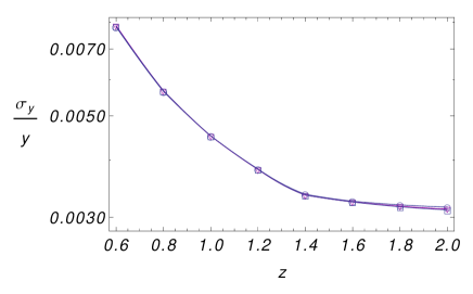
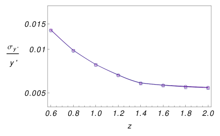
Figure 1: BAO mock data: fractional errors of BAO quantities $y(z)$ and $y^{\prime}(z)$ for the Euclid survey.

V Two-dimensional grid analysis

Given the appropriate $\chi^{2}(\boldsymbol{\theta})$ function we then proceed to find the values of the model parameters which minimize it. Using a grid (following prescriptions in numerical ) we study the parameter space of the model searching for the $\chi^{2}$ minimum. It is well known that when the number of parameters gets large, grid techniques require an increasing computational and time consuming effort, so it becomes preferable to use other statistical methods, such as Markov Chain Monte Carlo (MCMC). As we are going to explore two dark energy parameters only (with $\Omega_{m}$ and $\Omega_{b}$ fixed), the grid method is suitable for our purposes.

Combining some intuitive guesses with the knowledge provided by the vaste literature on the topic, we typically require just two grids (the second being finer and narrower) to find a suitable initial point to feed the Levenberg-Marquadt algorithm (described in full detail in numerical , pp.$\leavevmode\nobreak\ 683\leavevmode\nobreak\ -\leavevmode\nobreak\ 685$), and eventually detect the minimum $\chi^{2}$ value. In addition, the algorithm calculates the estimated covariance matrix $\mathbf{C}$ for the model parameters $\boldsymbol{\theta}$, which we use to plot the confidence regions in the 2-dimensional parameter space under the Gaussian approximation. This means that provided

$$\Delta\chi^{2}(\boldsymbol{\theta})=(\boldsymbol{\theta}-\boldsymbol{\theta_{\mathbf{best}}})^{T}\mathbf{C}^{-1}(\boldsymbol{\theta}-\boldsymbol{\theta_{\mathbf{best}}}),$$ (31)

the $1\sigma$ ($68.3\%$) and $2\sigma$ ($95.4\%$ confidence levels) will correspond to $\Delta\chi^{2}=2.30$ and $\Delta\chi^{2}=6.17$ respectively.

Finally, to compare results and test the issues of interest (in particular the tension among datasets), we compute the so called $\sigma$-distance, $d_{\sigma}$, i.e. the distance in units of $\sigma$ between the best fit points of the total sample and the best fit points of (respectively) SNeIa, BAO and a $\Lambda$CDM model corresponding to the different ($\Omega_{m}$,$\Omega_{b}$) pairs that define our priors. Following numerical , the $\sigma$-distance is calculated by solving

$$1-\Gamma(1,|\Delta\chi_{\sigma}^{2}/2|)/\Gamma(1)=\mathrm{erf}(d_{\sigma}/\sqrt{2}).$$ (32)

For homogeneity and consistency our “ruler” is in every case the total $\chi^{2}$ function ($\chi^{2}_{tot}=\chi^{2}_{\mathrm{SN}}+\chi^{2}_{\mathrm{BAO}}$), and our recipe is the following: if we want to calculate the tension between SNeIa and SNeIa+BAO and the best fit parameter vectors are respectively $\boldsymbol{\theta}_{\mathbf{SN}}$ and $\boldsymbol{\theta}_{\mathbf{SN+BAO}}$ then the previous $\Delta\chi_{\sigma}^{2}$ will be defined as $\chi_{tot}^{2}(\boldsymbol{\theta}_{\mathbf{SN+BAO}})-\chi_{tot}^{2}(\boldsymbol{\theta}_{\mathbf{SN}})$. Other cases follow simply from this prescription.

Table 5: Planck priors and CPL - Wang parametrization. Minimum correlation redshift $z_{c}$.

$\mathrm{Priors}$	$z_{c}\;\mathrm{(CPL/Wang)}$
$(\Omega_{m},\Omega_{b})$	SNeIa	BAO	SNeIa+BAO
$(0.214,0.0444)$	$0.226$	$0.113$	$0.220$
$(0.237,0.0444)$	$0.222$	$0.112$	$0.215$
$(0.260,0.0444)$	$0.217$	$0.112$	$0.210$
$(0.214,0.0405)$	$0.227$	$0.113$	$0.220$
$(0.237,0.0405)$	$0.222$	$0.112$	$0.216$
$(0.260,0.0405)$	$0.217$	$0.111$	$0.209$
$(0.214,0.0366)$	$0.226$	$0.112$	$0.221$
$(0.237,0.0366)$	$0.222$	$0.112$	$0.216$
$(0.260,0.0366)$	$0.217$	$0.111$	$0.210$

VI Results and Conclusions

As we have discussed in Sec. I, there are arguments suggesting that considering dark energy constraints from the combination of SNeIa and BAO data only is both relevant and useful, and so is comparing the individual predictions drawn from each other. This does not mean that we are going to avoid completely possible clues from the CMB analysis; in particular, the chosen priors for the cosmological density parameters $\Omega_{m}$ and $\Omega_{b}$ are derived from a forecast of CMB observations with the Planck satellite mission as reported in Burigana10 . The predicted best fits and $1\sigma$ errors are $\Omega_{m}h^{2}=0.1308\pm 0.0008$ and $\Omega_{b}h^{2}=0.0223$ which, combined with our choice for $h=0.742\pm 0.036$ from Riess09 , become $\Omega_{m}=0.237\pm 0.023$ and $\Omega_{b}=0.0405\pm 0.0039$. We then consider those best fits and combine them with their $1\sigma$ errors errors to produce nine $(\Omega_{m},\Omega_{b})$ couples. We then feed these priors into our pipeline so that we can describe quite in detail how the estimated EoS parameters depend on the uncertainties in $(\Omega_{m},\Omega_{b})$. Final results for current data are shown in Tables  (6) - (7), respectively for the CPL and Wang models; whereas forecasts for synthetic data can be examined by looking at Tables. (8) - (9).

Let us remind that Wang’s EoS model is based on the idea of obtaining a minimum correlation among its parameters. The pivot value $w_{0.5}$ is a conservative choice put forward in Wang:2008zh , which achieves quite a low degree of correlation and provides simple expression, although each single dataset or combination considered will have its own optimal correlation redshift which typically will not be too far away from Wang’s choice. The specific value of this pivot redshift can be easily calculated applying error propagation to the definition of $w_{c}$ in Eq. (6), and then computing the correlation parameters between $w_{0}$ and $w_{c}$ as a function of $a_{c}$ (or $z_{c}$) which one finally minimizes. For the CPL model the final expression is Wang:2008zh

$$a_{c}=1+\frac{\sigma^{2}(w_{0})}{\sigma^{2}(w_{0}w_{a})},$$ (33)

which clearly depends on the data set considered. For real data (see Tab. (6)), we effectively we detect a mean value of $z_{c}\approx 0.22-0.23$ using our chosen SNeIa data set, which gets only slightly reduced to $z_{c}\approx 0.21-0.22$ when considering the total sample SNeIa+BAO, and $z_{c}\approx 0.11$ for BAO data.

VI.1 Tension: results

The tension is confirmed both in the CPL and in the Wang case, and both with current and mock data; but it also shows different features with respect to references tensionfirsta ; tensionfirstb .

VI.1.1 Current data

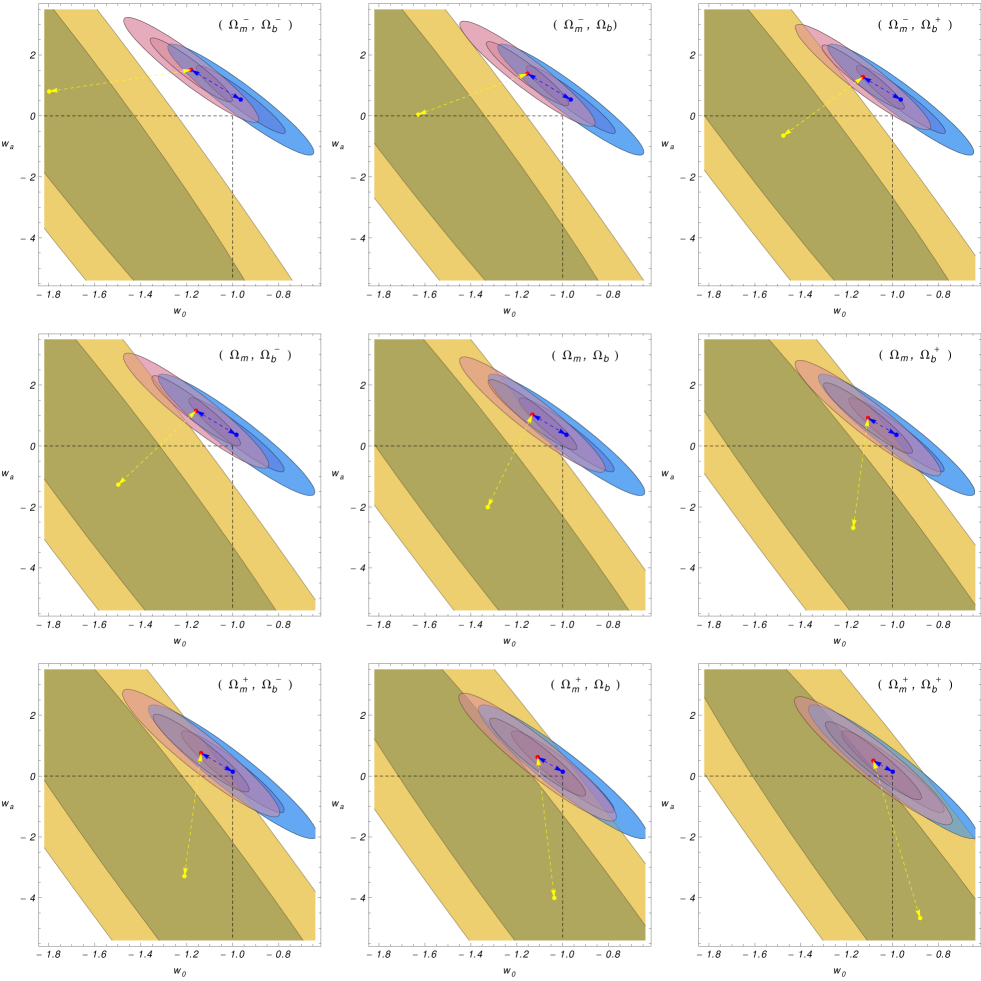
Figure 2: CPL model: 1$\sigma$ and 2$\sigma$ contours in the $w_{0}$-$w_{a}$ parameter space. In all plots SNeIa are represented by the blue region/point, BAO are the yellow region/point and the combined SNeIa-BAO are represented by the red region/point. The point where the dashed lines cross indicates the $\Lambda$CDM model. The arrows indicate the $\sigma$-distances for SNeIa and BAO, with the total $\chi^{2}$ as measure.

In these cases, SNeIa and BAO best fits can differ by more than $2\sigma$, as it is possible to conclude just by visual inspection from Figs. (2) - (3). When we compare the best fits from SNeIa alone and the SNeIa+BAO combination case we conclude there is no tension, as in all cases we have a separation smaller than $2\sigma$. On the contrary, there is always tension between BAO alone and SNeIa+BAO. Resorting again to visual examination we infer that for current data, the SNeIa+BAO credible intervals are very much influenced both in position and size by the SNeIa data, as these have much more statistical weight.

We can also underline another important property: the tension depends strongly on the value of the cosmological priors. In particular, we find a precise trend: the $\sigma$-distance between SNeIa and SNeIa+BAO best fits gets reduced either when $\Omega_{m}$ or $\Omega_{b}$ grow. In other words, compliance between SNeIa and BAO data improves when the amount of dark energy decreases, as has been noticed in earlier works biggerom . If $\Omega_{m}$ and $\Omega_{b}$ are large enough ($\Omega_{m}=0.260$ and $\Omega_{b}=0.0444,0.0405$), we even get close encounters (i.e. the distance among the best fits is less than $1\sigma$). The same trend holds true between SNeIa and BAO in the sense that the larger either $\Omega_{m}$ or $\Omega_{b}$ become, the larger the overlap between credible intervals.

As expected, there is large sensitivity to changes in $\Omega_{m}$ (from which both SNeIa and BAO depend) as compared to variations in $\Omega_{b}$ (which only influences BAO aspects). Note that BAO contours are much larger in size thus reflecting their statistically less meaningful character.

VI.1.2 Mock future data

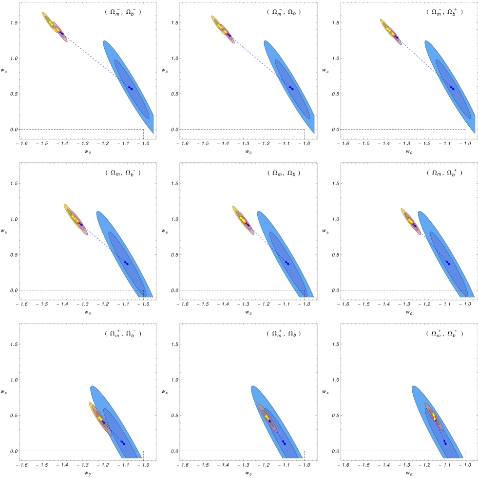
Figure 4: CPL model with CMB-oriented mock data: 1$\sigma$ and 2$\sigma$ contours in the $w_{0}$-$w_{a}$ parameter space. In all plots SNeIa are represented by the blue region/point, BAO are the yellow region/point and the combined SNeIa-BAO are represented by the red region/point. The point where the dashed lines cross indicates the $\Lambda$CDM model. The arrows indicate the $\sigma$-distances for SNeIa and BAO, with the total $\chi^{2}$ as measure.

When looking at mock data in Figs. (4) - (9), we get tension again, but now the role of SNeIa and BAO is inverted: the tension between SNeIa and SNeIa+BAO is always larger than $2\sigma$ while the tension between BAO and SNeIa+BAO is much less than $1\sigma$ when $\Omega_{m}$ has the largest and $\Omega_{b}$ has the two largest values.
Moreover, in this case the joint $\chi^{2}$ is clearly driven by BAO, exactly the opposite of the real data case. A possible explanation for this is that, as discussed in the related section, our mock data have been generated using different fiducial models, and two of them (the CMB and BAO-oriented case) have a constant value of $w$, below $-1$, even if with large errors). This choice clearly creates a bias in agreement with previous analyses: the fact that BAO are much keener with a phantom EoS than SNeIa, combined with the dramatically reduced errors drawn from expectations produce much smaller credible contours from BAO, very close in position and size to the total ones. In comparison, the statistical role of SNeIa is expected to become subdominant for future data.

On the other hand, we have to note that we have a BAO driven joint $\chi^{2}$ even in the SNeIa-oriented case, where $w\geq-1$. This may be put down to the fact that even in this case the smearing effect in the luminosity data is strong enough to make the data less informative than the BAO ones. The clear tension between SNeIa and BAO is somewhat surprising given that we have generated both synthetic datasets using exactly the same fiducial models. The element to have into consideration here is that the BAO data are divided in transverse and radial modes. The transverse modes share with SNeIa one fundamental property: they inform us on a quantity which depends on $w(z)$ through an integral (as can be seen in Eq. (33)), and this makes them less sensitive to changes in the EoS through the so-called smearing effect produced by the integration. Moreover the realistic dispersion of data around the fiducial model induces some dissociation from the underlying model. On the other hand, the radial modes depend directly on $w(z)$, so the BAO radial component can provide much more refined information.

Assuming the possibility of a substantial smearing effect, and considering the different statistical weights of SNeIa and BAO, one can wonder if there could possibly be a physical motivation for the tension among BAO and SNeIa, perhaps due to something not well established in the BAO or in the SNeIa data (for the SNeIa case, see Perivolaropoulos09 for a possible solution).

Finally, looking at the $\sigma-$distances we can also verify that the SNeIa-oriented model seems to be somewhat disfavored with respect to more phantom models, showing a larger tension (larger values for the $\sigma-$distances) with respect the other two cases.

VI.2 Dark energy evolution: results

There is a number of interesting conclusions about the EoS parameters which one can draw from a general overview of our figures and tables.

VI.2.1 Pivot choice and effect on errors

First of all, as Wang’s model is a reparametrization of the CPL model, it was to be expected that many similarities between them would be found. In particular, looking at the $\sigma-$distances, we see that they match each other perfectly. One can deduce that these two models are different projections in different parameter subspaces of a more general EoS parameters vector space (i.e. model). One piece of evidence highlighting the equivalence between between those scenarios is that the the estimations of $w_{0}$ are identical independently of the data used.

The main difference lies, obviously, in the EoS pivot parameter chosen: for CPL it is $w_{a}$, whereas Wang takes $w_{0.5}$. Although this cannot be falsified, intuition suggests Wang’s pivot is consistently chosen in a “redshift sense”, as it is informing us of a dark energy feature associated with a redshift value within the observationally described range. The CPL pivot parameter, on the other hand is typically very poorly constrained. Apart from the fact that the dark energy evolution in the CPL form is largely redshift independent asymptotically at high redshifts ($\lim_{z\to\infty}z/(z+1)=1$), we are questioning ourselves about a physically inaccessible dark energy feature, so it is not surprising that for this second dark energy parameter we get exceendingly large errors, as clearly reflected by our tables. Wang’s remedy improves the situation substantially; in fact percentual errors on $w_{0}$ and $w_{0.5}$ are of the same order of magnitude, whereas for $w_{a}$ they can even be one order of magnitude larger. This pattern is common to results coming from real and synthetic data.

VI.2.2 Dataset choices/combinations

In this subsection we look deeper into the results of our analysis to gain futher insight on the predictions from different datasets or their combination. This will allow us to draw more definitive conclusions about evolutionary features, to establish how convincing those conclusions are for current data, and to forecast what improvements are expected from future data. Likewise, these results will throw extra light on the effect of different prior choices (associated with the still considerable uncertainty in the determination of $\Omega_{m}$ and $\Omega_{b}$).

All real data SNeIa cases are $1\sigma$ compatible with $\Lambda$CDM. However, BAO data favour phantom models quite manifestly as their best fits are concerned, and the consequence is that for the SNeIa+CMB combination $\Lambda$CDM typically is marginally excluded at $1\sigma$, i.e. the case $w_{0}=-1$ lies outside the $1\sigma$ boundary but very close to it. Arguably, the phantomizing effect of BAO data is compensated by their large errors, and possible narrower error bands would yield a more decisive exlusion of $\Lambda$CDM.

Mock data, in contrast with real data, yield a picture in which $\Lambda$CDM is marginally excluded at $1\sigma$ by SNeIa data, whereas in the BAO and SNeIa+BAO cases the exclusion rate is considerable both because our mock BAO data favour more phantom models, and because the error bands are narrower.

On the other hand, dark energy subdominance at early times, i.e. $w_{\infty}=w_{0}+w_{a}<0$ is in general not guaranteed, and there are many cases (both for real and mock data) for which that situation is allowed at $1\sigma$. The main reason for this is that $w_{a}$ is rather poorly constrained. Specifically, for the SNeIa+BAO combination from real data and at the level of confidence we have just mentioned one can never guarantee $w_{\infty}<0$, whereas this is possible for some mock data cases. Another trend we observe is that the lowest values of $w_{\infty}$ correspond to $\Omega_{m}=0.260$, the largest value considered.

A related result is that for SNeIa the larger $\Omega_{m}$, the lower $w_{0}$; whereas for BAO the contrary happens and drives to the same behaviour for SNeIa+BAO (of course, unless we specify it otherwise, the same pattern is observed for real and mock data). This is as well a reflection of the tension between the two datasets. In constrast, increasing $\Omega_{m}$ induces always a decrease in $w_{a}$. As of $\Omega_{b}$ we can say that when it decreases, so does $w_{0}$, but the opposite happens to $w_{a}$.

In general, if $\Omega_{m}$ and $\Omega_{b}$ are fixed with independent observations, indeterminacies in their values can affect our conclusions about the current and early values of the dark energy parameter $w(z)$. The sensitivity to $\Omega_{m}$ is quite noticeable, and becomes particularly manifest for the $w_{a}$ parameter in the CPL case, whereas the situation is not so dramatic in Wang’s case. Note that even though Wang’s parametrization did not try to heal correlation between $\Omega_{m}$ and dark energy parameters, it comes out as a valuable consequence. This parametrization throws another interesting result: for real data and either $\Omega_{m}<0.260$ or $\Omega_{b}<0.044$ it can be ascertained at $1\sigma$ that acceleration has increased recently ($w$ has become more negative), whereas that situation occurs for mock data in all cases.

VI.3 Main conclusions

A number of relevant issues about dark energy have been explored using SNeIa and BAO observational data within the framework of the most popular representation of its possible evolution: the so called CPL model. The study is complemented by an in parallel consideration of a Wang’s reformulation of the former, as this is an advantageous alternative which minorates the correlation of parameters. Our main goals were to study whether there is tension between these two datasets, which are so far two of the most worthy tools to explore dark energy, and which are anticipated to play an even more preminent role in the future, particularly due to the spectacular advances expected in BAO astronomical data.

We have confirmed that tension is present in current data, and we have shown that, quite likely, it will be present in future data. Regarding this aspect of our work, it must be stressed that ours are the first time simulations of BAO data from both the radial and transverse directions in the literature.

In addition, we have paid considerable attention to the influence of indeterminacies in the values of $\Omega_{m}$ and $\Omega_{b}$ on the tension issue and other cosmodynamical questions such as whether dark energy is phantom-like, whether there has been an speed up in the acceleration of the universe, or whether dark energy could have perhaps been the dominant component at early times. Our main conclusions in this respect is that for most priors, and for the SNeIa+BAO combination best fits, the Universe is currently phantom-like, its dark energy EOS parameter has become more negative recently, and was dark matter dominated at early times.

Complementary conclusions are that future BAO data will improve constraints considerably making them far tighter, and Wang’s parametrization is a indeed a very good way to reformulate the CPL model and could become the dark energy parametrization of preferred use.

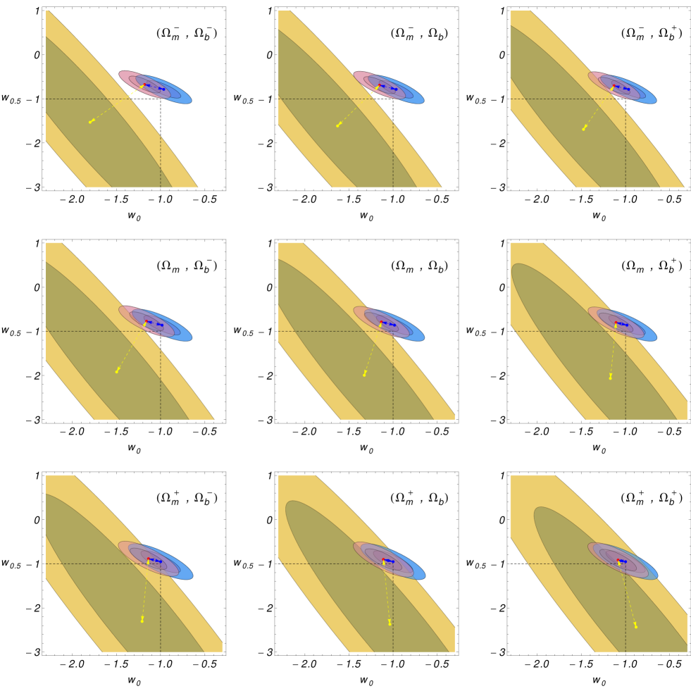
Figure 3: Wang model: 1$\sigma$ and 2$\sigma$ contours in the $w_{0}$-$w_{0.5}$ parameter space. In all plots SNeIa are represented by the blue region/point, BAO are the yellow region/point and the combined SNeIa-BAO are represented by the red region/point. The point where the dashed lines cross indicates the $\Lambda$CDM model. The arrows indicate the $\sigma$-distances for SNeIa and BAO, with the total $\chi^{2}$ as measure.

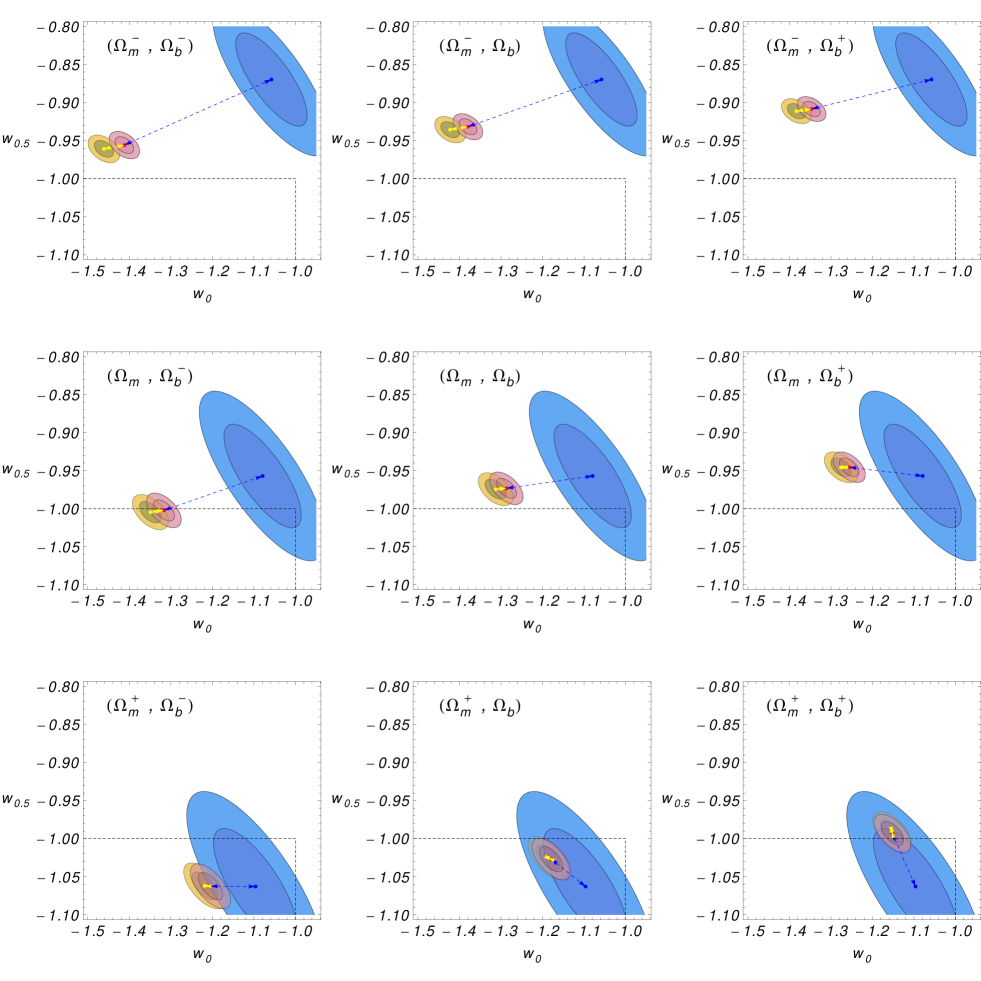
Figure 5: Wang model with CMB-oriented mock data: 1$\sigma$ and 2$\sigma$ contours in the $w_{0}$-$w_{0.5}$ parameter space. In all plots SNeIa are represented by the blue region/point, BAO are the yellow region/point and the combined SNeIa-BAO are represented by the red region/point. The point where the dashed lines cross indicates the $\Lambda$CDM model. The arrows indicate the $\sigma$-distances for SNeIa and BAO, with the total $\chi^{2}$ as measure.

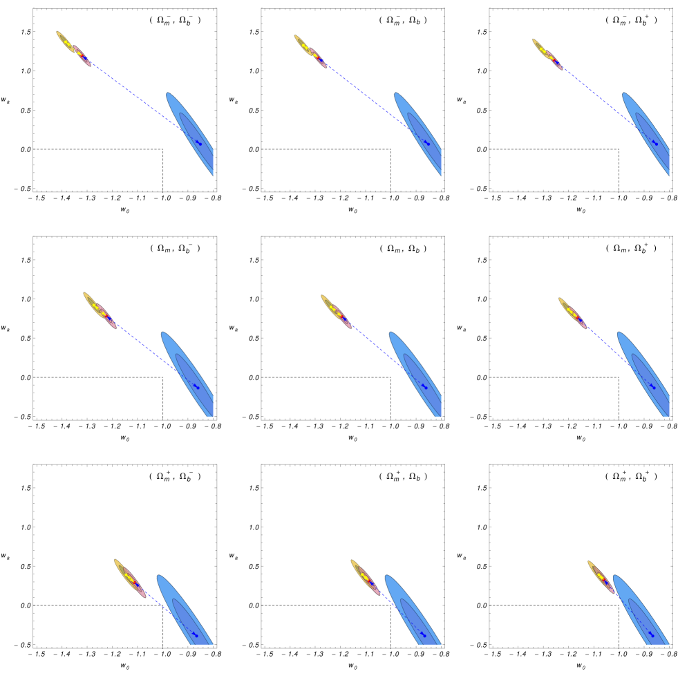
Figure 6: CPL model with SNeIa-oriented mock data: 1$\sigma$ and 2$\sigma$ contours in the $w_{0}$-$w_{a}$ parameter space. In all plots SNeIa are represented by the blue region/point, BAO are the yellow region/point and the combined SNeIa-BAO are represented by the red region/point. The point where the dashed lines cross indicates the $\Lambda$CDM model. The arrows indicate the $\sigma$-distances for SNeIa and BAO, with the total $\chi^{2}$ as measure.

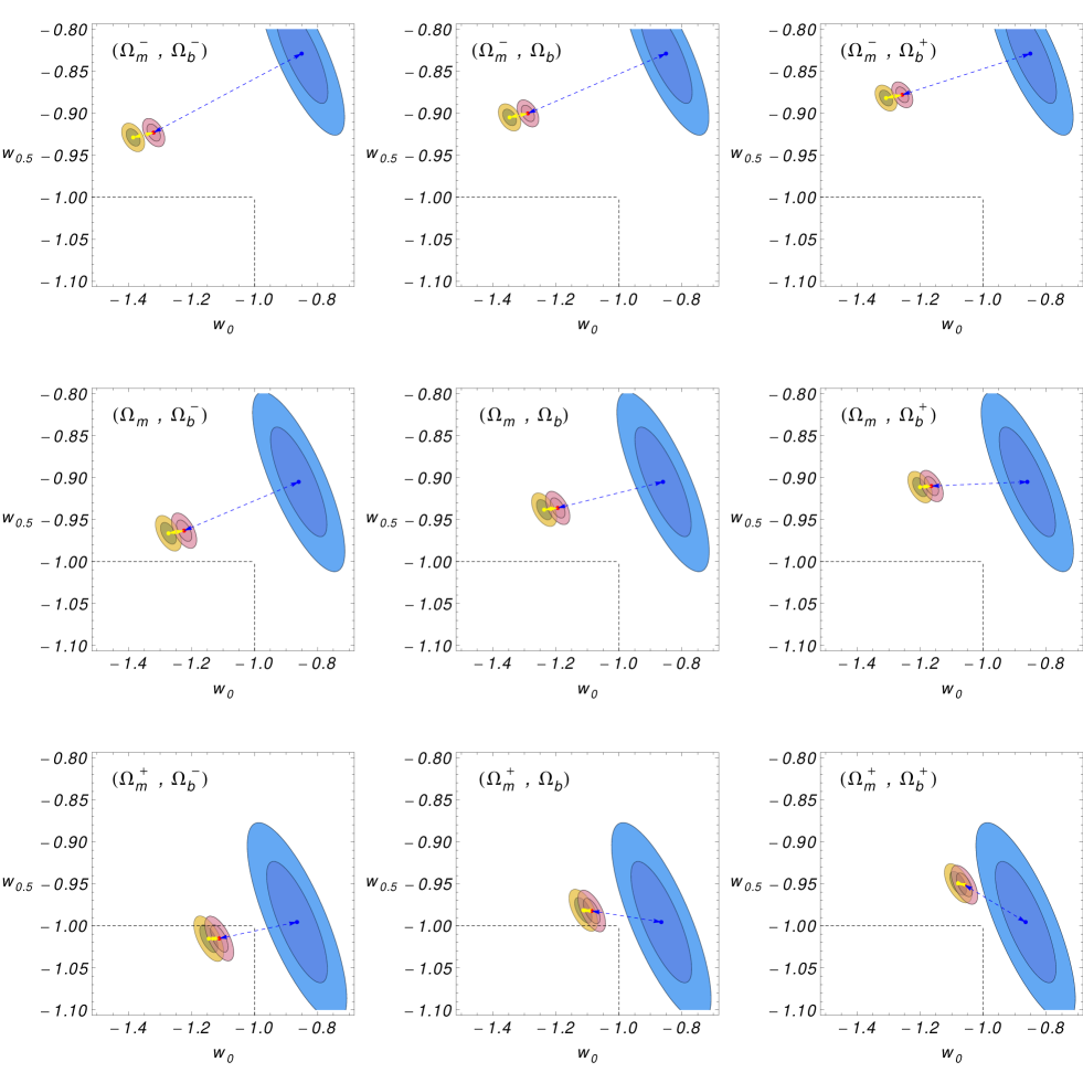
Figure 7: Wang model with SNeIa-oriented mock data: 1$\sigma$ and 2$\sigma$ contours in the $w_{0}$-$w_{0.5}$ parameter space. In all plots SNeIa are the blue region/point, BAO are the yellow region/point and the combined SNeIa-BAO are represented by the red region/point. The point where the dashed lines cross indicates the $\Lambda$CDM model. The arrows indicate the $\sigma$-distances for SNeIa and BAO, with the total $\chi^{2}$ as measure.

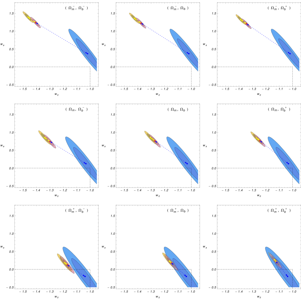
Figure 8: CPL model with BAO-oriented mock data: 1$\sigma$ and 2$\sigma$ contours in the $w_{0}$-$w_{a}$ parameter space. In all plots SNeIa are the blue region/point, BAO are the yellow region/point and the combined SNeIa-BAO are represented by the red region/point. The point where the dashed lines cross indicates the $\Lambda$CDM model. The arrows indicate the $\sigma$-distances for SNeIa and BAO, with the total $\chi^{2}$ as measure.

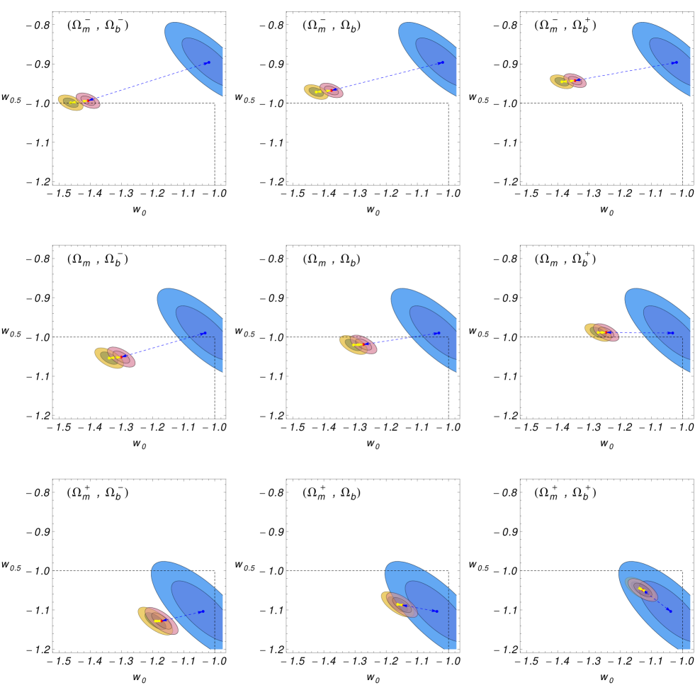
Figure 9: CPL model with BAO-oriented mock data: 1$\sigma$ and 2$\sigma$ contours in the $w_{0}$-$w_{a}$ parameter space. In all plots SNeIa are the blue region/point, BAO are the yellow region/point and the combined SNeIa-BAO are represented by the red region/point. The point where the dashed lines cross indicates the $\Lambda$CDM model. The arrows indicate the $\sigma$-distances for SNeIa and BAO, with the total $\chi^{2}$ as measure.

VII Acknowledgements

We acknowledge fruitful exchanges with Adam Amara, Bruce Bassett, Narciso Benítez, David Parkinson, Karl Glazebrook, Christopher Gordon, Thomas Kitching, Leandros Perivolaropoulos and Anais Rassat. Celia Escamilla-Rivera is supported by Fundación Pablo García and FUNDEC, México. Irene Sendra holds a PhD FPI fellowship-contract from the Spanish Ministry of Science and Innovation and Vincenzo Salzano holds a postdoctoral contract from the University of the Basque Country. Ruth Lazkoz, Vincenzo Salzano and Irene Sendra are supported by the Spanish Ministry of Science and Innovation through research projects FIS2010-15492 and Consolider EPI CSD2010-00064. The four authors are also supported by the Basque Government through the special research action AE-2010-1-31.

Table 6: CPL model and present data. Column. 1: prior choice; columns 2 - 3 - 4: best fit values of $w_{0}$ and $w_{a}$ for different datasets combinations; columns. 5 - 6 - 7 - 8: $d_{\sigma}$ calculated as described in Sec. (V) with respect to different datasets model.

$\mathrm{Priors}$	$\mathrm{Best\;fit\;parameters\;(w_{0},w_{a})}$			$\sigma-\mathrm{distances}$
$(\Omega_{m},\Omega_{b})$	SN	BAO	SN+BAO	$d_{\sigma}^{\mathrm{SN}}$	$d_{\sigma}^{\mathrm{BAO}}$	$d_{\sigma}^{\Lambda}$	$d_{\sigma}^{\mathrm{BAO-SN}}$
$(0.214,0.0444)$	$-0.965\pm 0.128$, $0.540\pm 0.736$	$-1.476\pm 0.713$, $-0.645\pm 6.955$	$-1.129\pm 0.119$, $1.278\pm 0.697$	$1.04$	$>3$	$1.96$	$>3$
$(0.237,0.0444)$	$-0.983\pm 0.137$, $0.367\pm 0.804$	$-1.171\pm 0.738$, $-2.687\pm 7.255$	$-1.107\pm 0.128$, $0.917\pm 0.765$	$0.62$	$>3$	$0.88$	$>3$
$(0.260,0.0444)$	$-0.999\pm 0.148$, $0.140\pm 0.885$	$-0.880\pm 0.763$, $-4.666\pm 7.568$	$-1.084\pm 0.138$, $0.503\pm 0.848$	$0.30$	$>3$	$0.21$	$>3$
$(0.214,0.0405)$	$-0.965\pm 0.128$, $0.540\pm 0.736$	$-1.629\pm 0.725$, $0.046\pm 7.099$	$-1.153\pm 0.119$, $1.389\pm 0.696$	$1.27$	$>3$	$1.98$	$>3$
$(0.237,0.0405)$	$-0.983\pm 0.137$, $0.367\pm 0.804$	$-1.326\pm 0.752$, $-2.009\pm 7.423$	$-1.132\pm 0.128$, $1.030\pm 0.764$	$0.81$	$>3$	$0.94$	$>3$
$(0.260,0.0405)$	$-0.999\pm 0.148$, $0.140\pm 0.885$	$-1.036\pm 0.779$, $-4.006\pm 7.762$	$-1.109\pm 0.138$, $0.620\pm 0.846$	$0.46$	$>3$	$0.34$	$>3$
$(0.214,0.0366)$	$-0.965\pm 0.128$, $0.540\pm 0.736$	$-1.799\pm 0.740$, $0.805\pm 7.272$	$-1.180\pm 0.119$, $1.514\pm 0.694$	$1.53$	$>3$	$2.03$	$>3$
$(0.237,0.0366)$	$-0.983\pm 0.137$, $0.367\pm 0.804$	$-1.498\pm 0.768$, $-1.269\pm 7.624$	$-1.159\pm 0.128$, $1.158\pm 0.762$	$1.05$	$>3$	$1.03$	$>3$
$(0.260,0.0366)$	$-0.999\pm 0.148$, $0.140\pm 0.885$	$-1.210\pm 0.798$, $-3.289\pm 7.997$	$-1.137\pm 0.138$, $0.752\pm 0.844$	$0.66$	$>3$	$0.52$	$>3$

Table 7: Wang model and present data. Column. 1: prior choice; columns 2 - 3 - 4: best fit values of $w_{0}$ and $w_{0.5}$ for different datasets combinations; columns. 5 - 6 - 7 - 8: $d_{\sigma}$ calculated as described in Sec. (V) with respect to different datasets model.

$\mathrm{Priors}$	$\mathrm{Best\;fit\;parameters\;(w_{0},w_{0.5})}$			$\sigma-\mathrm{distances}$
$(\Omega_{m},\Omega_{b})$	SN	BAO	SN+BAO	$d_{\sigma}^{\mathrm{SN}}$	$d_{\sigma}^{\mathrm{BAO}}$	$d_{\sigma}^{\Lambda\mathrm{CDM}}$	$d_{\sigma}^{\mathrm{BAO-SN}}$
$(0.214,0.0444)$	$-0.965\pm 0.128$, $-0.785\pm 0.132$	$-1.476\pm 0.713$, $-1.691\pm 1.640$	$-1.129\pm 0.119$, $-0.703\pm 0.128$	$1.04$	$>3$	$1.96$	$>3$
$(0.237,0.0444)$	$-0.983\pm 0.137$, $-0.861\pm 0.146$	$-1.171\pm 0.738$, $-2.067\pm 1.717$	$-1.107\pm 0.128$, $-0.802\pm 0.143$	$0.62$	$>3$	$0.88$	$>3$
$(0.260,0.0444)$	$-0.999\pm 0.148$, $-0.953\pm 0.164$	$-0.880\pm 0.763$, $-2.436\pm 1.797$	$-1.084\pm 0.138$, $-0.916\pm 0.161$	$0.30$	$>3$	$0.21$	$>3$
$(0.214,0.0405)$	$-0.965\pm 0.128$, $-0.785\pm 0.132$	$-1.629\pm 0.725$, $-1.613\pm 1.677$	$-1.153\pm 0.119$, $-0.690\pm 0.127$	$1.27$	$>3$	$1.98$	$>3$
$(0.237,0.0405)$	$-0.983\pm 0.137$, $-0.861\pm 0.146$	$-1.326\pm 0.752$, $-1.996\pm 1.759$	$-1.132\pm 0.128$, $-0.788\pm 0.142$	$0.81$	$>3$	$0.94$	$>3$
$(0.260,0.0405)$	$-0.999\pm 0.148$, $-0.953\pm 0.164$	$-1.036\pm 0.779$, $-2.372\pm 1.847$	$-1.109\pm 0.138$, $-0.902\pm 0.160$	$0.46$	$>3$	$0.34$	$>3$
$(0.214,0.0366)$	$-0.965\pm 0.128$, $-0.785\pm 0.132$	$-1.799\pm 0.740$, $-1.530\pm 1.720$	$-1.180\pm 0.119$, $-0.675\pm 0.127$	$1.53$	$>3$	$2.03$	$>3$
$(0.237,0.0366)$	$-0.983\pm 0.137$, $-0.861\pm 0.146$	$-1.498\pm 0.768$, $-1.921\pm 1.811$	$-1.159\pm 0.128$, $-0.773\pm 0.142$	$1.05$	$>3$	$1.03$	$>3$
$(0.260,0.0366)$	$-0.999\pm 0.148$, $-0.953\pm 0.164$	$-1.210\pm 0.798$, $-2.306\pm 1.907$	$-1.137\pm 0.138$, $-0.886\pm 0.160$	$>3$	$0.52$	$>3$

Table 8: CPL model and mock data. Column. 1: prior choice; columns 2 - 3 - 4: best fit values of $w_{0}$ and $w_{a}$ for different dataset combinations; columns. 5 - 6 - 7 - 8: $d_{\sigma}$ calculated as described in Sec. (V).

$\mathrm{CMB}-\mathrm{oriented}$
$\mathrm{Priors}$	$\mathrm{Best\;fit\;parameters\;(w_{0},w_{a})}$			$\sigma-\mathrm{distances}$
$(\Omega_{m},\Omega_{b})$	SN	BAO	SN+BAO	$d_{\sigma}^{\mathrm{SN}}$	$d_{\sigma}^{\mathrm{BAO}}$	$d_{\sigma}^{\Lambda\mathrm{CDM}}$	$d_{\sigma}^{\mathrm{BAO-SN}}$
$(0.214,0.0444)$	$-1.058\pm 0.057$, $0.565\pm 0.274$	$-1.383\pm 0.015$, $1.415\pm 0.055$	$-1.347\pm 0.014$, $1.314\pm 0.053$	$>3$	$2.62$	$>3$	$>3$
$(0.237,0.0444)$	$-1.079\pm 0.061$, $0.366\pm 0.299$	$-1.276\pm 0.016$, $0.990\pm 0.064$	$-1.256\pm 0.016$, $0.932\pm 0.063$	$>3$	$0.93$	$>3$	$>3$
$(0.260,0.0444)$	$-1.096\pm 0.067$, $0.100\pm 0.328$	$-1.153\pm 0.019$, $0.489\pm 0.078$	$-1.152\pm 0.018$, $0.476\pm 0.076$	$>3$	$0.06$	$>3$	$>3$
$(0.214,0.0405)$	$-1.058\pm 0.057$, $0.565\pm 0.274$	$-1.422\pm 0.015$, $1.460\pm 0.057$	$-1.380\pm 0.014$, $1.343\pm 0.055$	$>3$	$>3$	$>3$	$>3$
$(0.237,0.0405)$	$-1.079\pm 0.061$, $0.366\pm 0.299$	$-1.313\pm 0.017$, $1.015\pm 0.068$	$-1.287\pm 0.016$, $0.941\pm 0.066$	$>3$	$1.44$	$>3$	$>3$
$(0.260,0.0405)$	$-1.096\pm 0.067$, $0.100\pm 0.328$	$-1.187\pm 0.019$, $0.484\pm 0.083$	$-1.179\pm 0.019$, $0.456\pm 0.080$	$>3$	$0.11$	$>3$	$>3$
$(0.214,0.0366)$	$-1.058\pm 0.057$, $0.565\pm 0.274$	$-1.462\pm 0.015$, $1.502\pm 0.059$	$-1.412\pm 0.015$, $1.369\pm 0.058$	$>3$	$>3$	$>3$	$>3$
$(0.237,0.0366)$	$-1.079\pm 0.061$, $0.366\pm 0.299$	$-1.349\pm 0.017$, $1.034\pm 0.071$	$-1.317\pm 0.017$, $0.944\pm 0.069$	$>3$	$1.97$	$>3$	$>3$
$(0.260,0.0366)$	$-1.096\pm 0.067$, $0.100\pm 0.328$	$-1.219\pm 0.020$, $0.470\pm 0.089$	$-1.205\pm 0.019$, $0.427\pm 0.086$	$>3$	$0.42$	$>3$	$>3$
$\mathrm{BAO-oriented}$
$\mathrm{Priors}$	$\mathrm{Best\;fit\;parameters\;(w_{0},w_{a})}$			$\sigma-\mathrm{distances}$
$(\Omega_{m},\Omega_{b})$	SN	BAO	SN+BAO	$d_{\sigma}^{\mathrm{SN}}$	$d_{\sigma}^{\mathrm{BAO}}$	$d_{\sigma}^{\Lambda\mathrm{CDM}}$	$d_{\sigma}^{\mathrm{BAO-SN}}$
$(0.214,0.0444)$	$-1.019\pm 0.057$, $0.368\pm 0.278$	$-1.387\pm 0.015$, $1.324\pm 0.058$	$-1.344\pm 0.015$, $1.206\pm 0.057$	$>3$	$>3$	$>3$	$>3$
$(0.237,0.0444)$	$-1.031\pm 0.062$, $0.123\pm 0.304$	$-1.270\pm 0.017$, $0.845\pm 0.070$	$-1.245\pm 0.017$, $0.768\pm 0.069$	$>3$	$1.36$	$>3$	$>3$
$(0.260,0.0444)$	$-1.037\pm 0.067$, $-0.198\pm 0.333$	$-1.134\pm 0.020$, $0.265\pm 0.088$	$-1.127\pm 0.019$, $0.233\pm 0.085$	$>3$	$0.10$	$>3$	$>3$
$(0.214,0.0405)$	$-1.019\pm 0.057$, $0.368\pm 0.278$	$-1.425\pm 0.016$, $1.360\pm 0.061$	$-1.376\pm 0.015$, $1.225\pm 0.060$	$>3$	$>3$	$>3$	$>3$
$(0.237,0.0405)$	$-1.031\pm 0.062$, $0.123\pm 0.304$	$-1.305\pm 0.018$, $0.854\pm 0.074$	$-1.273\pm 0.017$, $0.761\pm 0.072$	$>3$	$1.89$	$>3$	$>3$
$(0.260,0.0405)$	$-1.037\pm 0.067$, $-0.198\pm 0.333$	$-1.163\pm 0.021$, $0.233\pm 0.094$	$-1.149\pm 0.020$, $0.186\pm 0.091$	$>3$	$0.36$	$>3$	$>3$
$(0.214,0.0366)$	$-1.019\pm 0.057$, $0.368\pm 0.278$	$-1.463\pm 0.016$, $1.391\pm 0.063$	$-1.407\pm 0.016$, $1.239\pm 0.062$	$>3$	$>3$	$>3$	$>3$
$(0.237,0.0366)$	$-1.031\pm 0.062$, $0.123\pm 0.304$	$-1.339\pm 0.019$, $0.855\pm 0.079$	$-1.300\pm 0.018$, $0.746\pm 0.077$	$>3$	$2.43$	$>3$	$>3$
$(0.260,0.0366)$	$-1.037\pm 0.067$, $-0.198\pm 0.333$	$-1.190\pm 0.022$, $0.186\pm 0.102$	$-1.171\pm 0.021$, $0.128\pm 0.098$	$>3$	$0.79$	$>3$	$>3$
$\mathrm{SNeIa-oriented}$
$\mathrm{Priors}$	$\mathrm{Best\;fit\;parameters\;(w_{0},w_{a})}$			$\sigma-\mathrm{distances}$
$(\Omega_{m},\Omega_{b})$	SN	BAO	SN+BAO	$d_{\sigma}^{\mathrm{SN}}$	$d_{\sigma}^{\mathrm{BAO}}$	$d_{\sigma}^{\Lambda\mathrm{CDM}}$	$d_{\sigma}^{\mathrm{BAO-SN}}$
$(0.214,0.0444)$	$-0.850\pm 0.055$, $0.064\pm 0.266$	$-1.308\pm 0.014$, $1.280\pm 0.052$	$-1.257\pm 0.013$, $1.137\pm 0.051$	$>3$	$>3$	$>3$	$>3$
$(0.237,0.0444)$	$-0.860\pm 0.059$, $-0.136\pm 0.289$	$-1.200\pm 0.016$, $0.867\pm 0.061$	$-1.164\pm 0.015$, $0.762\pm 0.060$	$>3$	$2.39$	$>3$	$>3$
$(0.260,0.0444)$	$-0.865\pm 0.064$, $-0.390\pm 0.314$	$-1.080\pm 0.018$, $0.391\pm 0.072$	$-1.060\pm 0.017$, $0.325\pm 0.071$	$>3$	$0.81$	$>3$	$>3$
$(0.214,0.0405)$	$-0.850\pm 0.055$, $0.064\pm 0.266$	$-1.347\pm 0.014$, $1.326\pm 0.054$	$-1.289\pm 0.014$, $1.166\pm 0.053$	$>3$	$>3$	$>3$	$>3$
$(0.237,0.0405)$	$-0.860\pm 0.059$, $-0.136\pm 0.289$	$-1.237\pm 0.016$, $0.897\pm 0.064$	$-1.194\pm 0.015$, $0.774\pm 0.062$	$>3$	$2.93$	$>3$	$>3$
$(0.260,0.0405)$	$-0.865\pm 0.064$, $-0.390\pm 0.314$	$-1.113\pm 0.018$, $0.395\pm 0.077$	$-1.086\pm 0.018$, $0.312\pm 0.075$	$>3$	$1.30$	$>3$	$>3$
$(0.214,0.0366)$	$-0.850\pm 0.055$, $0.064\pm 0.266$	$-1.385\pm 0.015$, $1.370\pm 0.056$	$-1.320\pm 0.014$, $1.192\pm 0.055$	$>3$	$>3$	$>3$	$>3$
$(0.237,0.0366)$	$-0.860\pm 0.059$, $-0.136\pm 0.289$	$-1.273\pm 0.017$, $0.921\pm 0.067$	$-1.224\pm 0.016$, $0.781\pm 0.065$	$>3$	$>3$	$>3$	$>3$
$(0.260,0.0366)$	$-0.865\pm 0.064$, $-0.390\pm 0.314$	$-1.145\pm 0.019$, $0.390\pm 0.081$	$-1.112\pm 0.018$, $0.291\pm 0.079$	$>3$	$1.82$	$>3$	$>3$

Table 9: Wang model and mock data. Column. 1: prior choice; columns 2 - 3 - 4: best fit values of $w_{0}$ and $w_{0.5}$ for different dataset combinations; columns. 5 - 6 - 7 - 8: $d_{\sigma}$ calculated as described in Sec. (V).

$\mathrm{CMB}-\mathrm{oriented}$
$\mathrm{Priors}$	$\mathrm{Best\;fit\;parameters\;(w_{0},w_{0.5})}$			$\sigma-\mathrm{distances}$
$(\Omega_{m},\Omega_{b})$	SN	BAO	SN+BAO	$d_{\sigma}^{\mathrm{SN}}$	$d_{\sigma}^{\mathrm{BAO}}$	$d_{\sigma}^{\Lambda\mathrm{CDM}}$	$d_{\sigma}^{\mathrm{BAO-SN}}$
$(0.214,0.0444)$	$-1.058\pm 0.057$, $-0.870\pm 0.040$	$-1.383\pm 0.015$, $-0.911\pm 0.007$	$-1.347\pm 0.014$, $-0.908\pm 0.007$	$>3$	$2.62$	$>3$	$>3$
$(0.237,0.0444)$	$-1.079\pm 0.061$, $-0.957\pm 0.045$	$-1.276\pm 0.016$, $-0.946\pm 0.008$	$-1.256\pm 0.016$, $-0.946\pm 0.008$	$>3$	$0.93$	$>3$	$>3$
$(0.260,0.0444)$	$-1.096\pm 0.067$, $-1.063\pm 0.050$	$-1.153\pm 0.019$, $-0.990\pm 0.010$	$-1.152\pm 0.018$, $-0.993\pm 0.010$	$>3$	$0.06$	$>3$	$>3$
$(0.214,0.0405)$	$-1.058\pm 0.057$, $-0.870\pm 0.040$	$-1.422\pm 0.015$, $-0.936\pm 0.007$	$-1.380\pm 0.014$, $-0.932\pm 0.007$	$>3$	$>3$	$>3$	$>3$
$(0.237,0.0405)$	$-1.079\pm 0.061$, $-0.957\pm 0.045$	$-1.313\pm 0.017$, $-0.974\pm 0.009$	$-1.287\pm 0.016$, $-0.973\pm 0.009$	$>3$	$1.44$	$>3$	$>3$
$(0.260,0.0405)$	$-1.096\pm 0.067$, $-1.063\pm 0.050$	$-1.187\pm 0.019$, $-1.025\pm 0.011$	$-1.179\pm 0.019$, $-1.027\pm 0.011$	$>3$	$0.11$	$>3$	$>3$
$(0.214,0.0366)$	$-1.058\pm 0.057$, $-0.870\pm 0.040$	$-1.462\pm 0.015$, $-0.961\pm 0.007$	$-1.412\pm 0.015$, $-0.956\pm 0.007$	$>3$	$>3$	$>3$	$>3$
$(0.237,0.0366)$	$-1.079\pm 0.061$, $-0.957\pm 0.045$	$-1.349\pm 0.017$, $-1.005\pm 0.009$	$-1.317\pm 0.017$, $-1.002\pm 0.009$	$>3$	$1.97$	$>3$	$>3$
$(0.260,0.0366)$	$-1.096\pm 0.067$, $-1.063\pm 0.050$	$-1.219\pm 0.020$, $-1.062\pm 0.012$	$-1.205\pm 0.019$, $-1.062\pm 0.012$	$>3$	$0.42$	$>3$	$>3$
$\mathrm{BAO-oriented}$
$\mathrm{Priors}$	$\mathrm{Best\;fit\;parameters\;(w_{0},w_{0.5})}$			$\sigma-\mathrm{distances}$
$(\Omega_{m},\Omega_{b})$	SN	BAO	SN+BAO	$d_{\sigma}^{\mathrm{SN}}$	$d_{\sigma}^{\mathrm{BAO}}$	$d_{\sigma}^{\Lambda\mathrm{CDM}}$	$d_{\sigma}^{\mathrm{BAO-SN}}$
$(0.214,0.0444)$	$-1.019\pm 0.057$, $-0.896\pm 0.041$	$-1.387\pm 0.015$, $-0.945\pm 0.007$	$-1.344\pm 0.015$, $-0.942\pm 0.007$	$>3$	$>3$	$>3$	$>3$
$(0.237,0.0444)$	$-1.031\pm 0.062$, $-0.990\pm 0.046$	$-1.270\pm 0.017$, $-0.989\pm 0.009$	$-1.245\pm 0.017$, $-0.988\pm 0.009$	$>3$	$1.36$	$>3$	$>3$
$(0.260,0.0444)$	$-1.037\pm 0.067$, $-1.104\pm 0.051$	$-1.134\pm 0.020$, $-1.046\pm 0.012$	$-1.127\pm 0.019$, $-1.049\pm 0.012$	$>3$	$0.10$	$>3$	$>3$
$(0.214,0.0405)$	$-1.019\pm 0.057$, $-0.896\pm 0.041$	$-1.425\pm 0.016$, $-0.972\pm 0.008$	$-1.376\pm 0.015$, $-0.968\pm 0.007$	$>3$	$>3$	$>3$	$>3$
$(0.237,0.0405)$	$-1.031\pm 0.062$, $-0.990\pm 0.046$	$-1.305\pm 0.018$, $-1.020\pm 0.010$	$-1.273\pm 0.017$, $-1.019\pm 0.010$	$>3$	$1.89$	$>3$	$>3$
$(0.260,0.0405)$	$-1.037\pm 0.067$, $-0.198\pm 0.333$	$-1.163\pm 0.021$, $-1.086\pm 0.013$	$-1.149\pm 0.020$, $-1.087\pm 0.013$	$>3$	$0.36$	$>3$	$>3$
$(0.214,0.0366)$	$-1.019\pm 0.057$, $-0.896\pm 0.041$	$-1.463\pm 0.016$, $-0.999\pm 0.063$	$-1.407\pm 0.016$, $-0.994\pm 0.008$	$>3$	$>3$	$>3$	$>3$
$(0.237,0.0366)$	$-1.031\pm 0.062$, $-0.990\pm 0.046$	$-1.339\pm 0.019$, $-1.054\pm 0.010$	$-1.300\pm 0.018$, $-1.051\pm 0.010$	$>3$	$2.43$	$>3$	$>3$
$(0.260,0.0366)$	$-1.037\pm 0.067$, $-1.104\pm 0.051$	$-1.190\pm 0.022$, $-1.128\pm 0.014$	$-1.171\pm 0.021$, $-1.128\pm 0.014$	$>3$	$0.79$	$>3$	$>3$
$\mathrm{SNeIa-oriented}$
$\mathrm{Priors}$	$\mathrm{Best\;fit\;parameters\;(w_{0},w_{0.5})}$			$\sigma-\mathrm{distances}$
$(\Omega_{m},\Omega_{b})$	SN	BAO	SN+BAO	$d_{\sigma}^{\mathrm{SN}}$	$d_{\sigma}^{\mathrm{BAO}}$	$d_{\sigma}^{\Lambda\mathrm{CDM}}$	$d_{\sigma}^{\mathrm{BAO-SN}}$
$(0.214,0.0444)$	$-0.850\pm 0.055$, $-0.829\pm 0.039$	$-1.308\pm 0.014$, $-0.882\pm 0.006$	$-1.257\pm 0.013$, $-0.878\pm 0.006$	$>3$	$>3$	$>3$	$>3$
$(0.237,0.0444)$	$-0.860\pm 0.059$, $-0.905\pm 0.043$	$-1.200\pm 0.016$, $-0.911\pm 0.008$	$-1.164\pm 0.015$, $-0.910\pm 0.007$	$>3$	$2.39$	$>3$	$>3$
$(0.260,0.0444)$	$-0.865\pm 0.064$, $-0.995\pm 0.048$	$-1.080\pm 0.018$, $-0.949\pm 0.009$	$-1.060\pm 0.017$, $-0.951\pm 0.009$	$>3$	$0.81$	$>3$	$>3$
$(0.214,0.0405)$	$-0.850\pm 0.055$, $-0.829\pm 0.039$	$-1.347\pm 0.014$, $-0.905\pm 0.006$	$-1.289\pm 0.014$, $-0.900\pm 0.006$	$>3$	$>3$	$>3$	$>3$
$(0.237,0.0405)$	$-0.860\pm 0.059$, $-0.905\pm 0.043$	$-1.237\pm 0.016$, $-0.938\pm 0.008$	$-1.194\pm 0.015$, $-0.936\pm 0.008$	$>3$	$2.93$	$>3$	$>3$
$(0.260,0.0405)$	$-0.865\pm 0.064$, $-0.995\pm 0.048$	$-1.113\pm 0.018$, $-0.981\pm 0.010$	$-1.086\pm 0.018$, $-0.982\pm 0.010$	$>3$	$1.30$	$>3$	$>3$
$(0.214,0.0366)$	$-0.850\pm 0.055$, $-0.829\pm 0.039$	$-1.385\pm 0.015$, $-0.929\pm 0.007$	$-1.320\pm 0.014$, $-0.923\pm 0.007$	$>3$	$>3$	$>3$	$>3$
$(0.237,0.0366)$	$-0.860\pm 0.059$, $-0.905\pm 0.043$	$-1.273\pm 0.017$, $-0.966\pm 0.009$	$-1.224\pm 0.016$, $-0.963\pm 0.008$	$>3$	$>3$	$>3$	$>3$
$(0.260,0.0366)$	$-0.865\pm 0.064$, $-0.995\pm 0.048$	$-1.145\pm 0.019$, $-1.015\pm 0.011$	$-1.112\pm 0.018$, $-1.015\pm 0.011$	$>3$	$1.82$	$>3$	$>3$

References

- (1) A.G. Riess, et al., Astrophys. J. 116 (1998) 1009; S. Perlmutter, et al., Astrophys. J. 517 (1999) 565; A.G. Riess, et al. Astrophys. J. 607 (2004) 665; P. Astier, et al., Astron. Astrophys. 447 (2006) 31; A. Clocchiati, et al., Astrophys. J. 642 (2006) 1.
- (2) D.N. Spergel, et al., Astrophys. J. Suppl. 170 (2007); A.C.S. Readhead, et al., Astrophys. J. 609 (2004) 498; J.H. Goldstein, et al., Astrophys. J. 599 (2003) 773; R. Rebolo, et al., Mon. Not. R. Astron. Soc. 353 (2004) 747; M. Tegmark, et al., Phys. Rev. D 69 (2004); E. Hawkins, et al., Mon. Not. R. Astron. Soc. 346 (2003).
- (3) V.R. Eke, S. Cole, C.S. Frenk, H.J. Petrick, Mon. Not. R. Astron. Soc. 298 (1998) 1145; P.T.P. Viana, R.C. Nichol, A.R. Liddle, Astrophys. J. 569 (2002) 75; N.A. Bahcall, et al., Astrophys. J. 585 (2003) 182; N.A. Bahcall, P. Bode, Astrophys. J. 588 (2003) 1.
- (4) A.C. Pope, et al., Astrophys. J. 607 (2005) 655; S. Cole, et al., Mon. Not. R. Astron. Soc. 362 (2005) 505; D. Eisenstein, et al., Astrophys. J. 633 (2005) 560.
- (5) P. de Bernardis, et al., Nature 404 (2000) 955; D.N. Spergel, et al., Astrophys. J. Suppl. 148 (2003) 175.
- (6) E. Komatsu, et al., Astrophys. J. Suppl. 192 (2011) 18.
- (7) L. van Waerbecke, et al., Astron. Astrophys. 374 (2001) 757; A. Refregier, Ann. Rev. Astron. Astrophys. 41 (2003) 645.
- (8) R.A.C. Croft, W. Hu,R. Dave, Phys. Rev. Lett. 83 (1999) 1092; P. McDonald, et al., Astrophys. J. 635 (2005) 761.
- (9) S.M. Carroll, W.H. Press, E.L. Turner, Ann. Rev. Astron. Astrophys. 30 (1992) 499.
- (10) V. Sahni, A. Starobinski, Int. J. Mod. Phys. D 9 (2000) 373.
-
(11)
http://lambda.gsfc.nasa.gov/product/map/current
/parameters.cfm. - (12) M. Tegmark, et al., Phys. Rev. D 69 (2004) 103501; U. Seljak, et al., Phys. Rev. D 71 (2005) 103515; A.G. Sanchez, et al., Mon. Not. R. Astron. Soc. 366 (2006) 189.
- (13) A.R. Liddle, “An introduction to modern cosmology”, Chichester, UK: Wiley, 1998.
- (14) M. Chevallier, D. Polarski, David, Int. J. Mod. Phys. D 10 (2001) 213.
- (15) S. Tsujikawa, arXiv:1004.1493; G. Dvali, New J. Phys. 8 (2006) 326; S.M. Carroll, A. De Felice, V. Duvvuri, D.A. Easson, M. Trodden, M.S. Turner, Phys. Rev. D 71 (2005) 063513; C. Escamilla-Rivera, O. Obregon, L.A. Urena-Lopez, J. Cosmol. Astropart. P. 1012 (2010) 011.
- (16) K. Freese, M. Lewis, Phys. Lett. B 540 (2002) 1.
- (17) V. Gorini, A. Kamenshchik, U. Moschella, Phys. Rev. D 67 (2003) 063509; M.C. Bento, O. Bertolami, A.A. Sen, Phys. Rev. D 66 (2002) 043507.
- (18) V. Sahni, Y.Shtanov, J. Cosmol. Astropart. P. 0311 (2003) 014; R. Maartens, J. Phys. Conf. Ser. 68 (2007) 012046.
- (19) T.P. Sotiriou, V. Faraoni, Rev. Mod. Phys. 82 (2010) 451.
- (20) A. Albrecht, L. Amendola, G. Bernstein, D. Clowe, D. Eisenstein, L. Guzzo, C. Hirata, D. Huterer, et al., arXiv:0901.0721.
- (21) S. Nesseris, L. Perivolaropoulos, J. Cosmol. Astropart. P. 0702 (2007) 025.
- (22) M. Li, X.-D. Li, S. Wang, arXiv:0910.0717; H. Wei, Phys. Lett. B 687 (2010) 286; Bengochea, Gabriel R. Phys. Lett. B 696 (2011); Li, Zhengxiang, et-al. Phys. Lett. B 695 (2011).
- (23) R. Lazkoz, S. Nesseris, and L. Perivolaropoulos, L., J. Cosmol. Astropart. P. 0807 (2008) 012.
- (24) Y.G. Gong, Y.Z. Zhang, Phys. Rev. D 72 (2005) 043518; H.K. Jassal, J.S. Bagla, T. Padmanabhan, Mon. Not. R. Astron. Soc. 356 (2005) L11; T. Padmanabhan, T.R. Choudhury, Mon. Not. R. Astron. Soc. 344 (2003) 823; D. Huterer, M.S. Turner, Phys. Rev. D 64 (2001) 123527; T.R. Choudhury, T. Padmanabhan, T., Astron. Astrophys. 429 (2005) 807; C. Wetterich, Phys. Lett. B 594 (2004) 17; A. Upadhye, M. Ishak, P.J. Steinhardt, Phys. Rev. D 72 (2005) 063501; S. Lee, Phys. Rev. D 71 (2005) 123528; P. Barai, T.K. Das, P.J. Wiita, Astrophys. J. 613 (2004) L49; E.V. Linder, Phys. Rev. D 73 (2006) 063010; R. Lazkoz, V. Salzano, I. Sendra, Phys. Lett. B 694 (2010) 198; J.-Z. Ma, X. Zhang, Phys. Lett. B 699 (2011) 233.
- (25) A. Albrecht, astro-ph/0609591.
- (26) E.V. Linder, Phys. Rev. Lett. 90 (2003) 091301.
- (27) Y. Wang, Phys. Rev. D 77 (2008) 123525.
- (28) A. Zitrin, et al., arXiv:1103.5618.
- (29) J.C. Bueno-Sanchez, S. Nesseris, L. Perivolaropoulos, L., J. Cosmol. Astropart. P. 0911 (2009) 029.
- (30) Y. Wang, et al., Mon. Not. R. Astron. Soc. 409 (2010) 737.
- (31) C. Blake, et al., Mon. Not. R. Astron. Soc. 365 (2006) 255.
- (32) D.G. York, et al., Astrophys. J. 120 (2000) 1579.
- (33) K. Abazajian, et al., Astrophys. J. Supp. S. 182 (2009) 543.
- (34) M. Colless, et al., astro-ph/0306581.
- (35) R. Amanullah, et al., Astrophys. J. 716 (2010) 712.
- (36) M. Kowalski, D. Rubin, G. Aldering, et al., Astrophys. J. 686 (2008) 749.
- (37) R. Amanullah, et al., Astron. Astrophys. 486 (2008) 375.
- (38) M. Hicken, et al., Astrophys. J. 700 (2009) 331.
- (39) J.A. Holtzman, et al., Astron. J. 136 (2009) 2306.
- (40) E. Di Pietro, J.F. Claeskens, Mon. Not. Roy. Astron. Soc. 341 (2003) 1299; S. Nesseris, L. Perivolaropoulos, Phys. Rev. D 70 (2004) 043531; O. Elgaroy, T. Multamki, J. Cosmol. Astropart. P. 0609 (2006) 002.
- (41) P.S. Corasaniti, A. Melchiorri, Phys. Rev. D 77 (2008) 103507; Y. Wang, P. Mukherjee, Phys. Rev.D 76, (2007) 103533.
- (42) W.J. Percival, et al., Mon. Not. R. Astron. Soc. 401 (2010) 2148.
- (43) H.J. Seo, D.J. Eisenstein, Astrophys. J 665 (2007) 14.
- (44) D. Coe, arXiv:0906.4123.
- (45) E. Komatsu, et al., Astrophys. J. Supp. S. 180 (2009) 330.
- (46) A. Refregier, A. Amara, T. Kitching, A. Rassat, Astron. Astrophys. 528 (2011) 33.
- (47) A. Albrecht, et al., arXiv:0901.0721.
-
(48)
G. Aldering, et al., http://snfactory.lbl.gov/snf/pdf/
spie2002.pdf. - (49) A.G. Kim, E.V. Linder, R. Miquel, N. Mostek, Mon. Not. R. Astron. Soc. 347 (2004) 909; A. Upadhye, M. Ishak, P. Steinhardt, Phys. Rev. D 72 (2005) 063501; M. Ishak, Found. Phys. 37 (2007) 1470.
-
(50)
http://lambda.gsfc.nasa.gov/product/map/dr4/params
/wcdm_sz_lens_wmap7.cfm. - (51) G. Efstathiou, J.R. Bond, Mon. Not. R. Astron. Soc. 304 (1999) 75; W. Hu, N. Sugiyama, Astrophys. J. 471 (1996) 542.
- (52) M. Martinelli, E. Calabrese, F. De Bernardis, A. Melchiorri, L. Pagano, et al., Phys. Rev. D 83 (2011) 023012; J.P. Beaulieu, D.P. Bennett, V. Batista, A. Cassan, D. Kubas, et al., arXiv:1001.3349; A. Refregier, et al., arXiv:1001.0061; http://sci.esa.int/euclid.
- (53) W.H. Press, et.al., “Numerical Recipes”, Cambridge Press, 1994.
- (54) C. Burigana, et al., Astrophys. J. 724 (2010) 588.
- (55) A.G. Riess, et al., Astrophys. J. 699 (2009) 539.
- (56) J.C.B. Sanchez, S. Nesseris, L. Perivolaropoulos, J. Cosmol. Astropart. P. 0911 (2009) 029; A. Shafieloo, V. Sahni, A.A. Starobinsky, Phys. Rev. D 80 (2009) 101301.
- (57) L. Perivolaropoulos, A. Shafieloo, Phys. Rev. D 79 (2009) 123502.