Exact energy of the spin-polarized two-dimensional electron gas at high density

Abstract

We derive the exact expansion, to $O(r_{s})$, of the energy of the high-density spin-polarized two-dimensional uniform electron gas, where $r_{s}$ is the Seitz radius.

The three-dimensional uniform electron gas is a ubiquitous paradigm in solid-state physics Kohn (1999) and quantum chemistry, Pople (1999) and has been extensively used as a starting point in the development of exchange-correlation density functionals in the framework of density-functional theory. Parr and Yang (1989) The two-dimensional version of the electron gas has also been the object of extensive research Ando et al. (1982); Abrahams et al. (2001) because of its intimate connection to two-dimensional or quasi-two-dimensional materials, such as quantum dots. Alhassid (2000); Reimann and Manninen (2002)

The two-dimensional gas (or 2-jellium) is characterized by a density $\rho=\rho_{\uparrow}+\rho_{\downarrow}$, where $\rho_{\uparrow}$ and $\rho_{\downarrow}$ are the (uniform) densities of the spin-up and spin-down electrons, respectively. In order to guarantee its stability, the electrons are assumed to be embedded in a uniform background of positive charge. Giuliani and Vignale (2005) We will use atomic units throughout.

It is known from contributions by numerous workers Misawa (1965); Stern (1973); Zia (1973); Isihara and Toyoda (1977); Rajagopal and Kimball (1977); Isihara and Ioriatti (1980); Tanatar and Ceperley (1989); Attaccalite et al. (2002); Seidl (2004); Chesi and Giuliani (2007); Drummond and Needs (2009) that the high-density (i.e. small-$r_{s}$) expansion of the energy per electron (or reduced energy) in 2-jellium is

$$E(r_{s},\zeta)=\frac{\varepsilon_{-2}(\zeta)}{r_{s}^{2}}+\frac{\varepsilon_{-1}(\zeta)}{r_{s}}+\varepsilon_{0}(\zeta)+\varepsilon_{\ell}(\zeta)\,r_{s}\ln r_{s}+O(r_{s}),$$ (1)

where $r_{s}=\left(\pi\rho\right)^{-1/2}$ is the Seitz radius, and

$$\zeta=\frac{\rho_{\uparrow}-\rho_{\downarrow}}{\rho}$$ (2)

is the relative spin polarization. Giuliani and Vignale (2005) Without loss of generality, we assume $\rho_{\downarrow}\leq\rho_{\uparrow}$, i.e. $\zeta\in[0,1]$.

The first two terms of the expansion (1) are the kinetic and exchange energies, and their sum gives the Hartree-Fock (HF) energy. The paramagnetic ($\zeta=0$) coefficients are

$$\varepsilon_{-2}(0) =+\frac{1}{2},$$ (3)

$$\varepsilon_{-1}(0) =-\frac{4\sqrt{2}}{3\pi},$$ (4)

and their spin-scaling functions are

$$\Upsilon_{-2}(\zeta) =\frac{\varepsilon_{-2}(\zeta)}{\varepsilon_{-2}(0)}=\frac{(1-\zeta)^{2}+(1+\zeta)^{2}}{2},$$ (5)

$$\Upsilon_{-1}(\zeta) =\frac{\varepsilon_{-1}(\zeta)}{\varepsilon_{-1}(0)}=\frac{(1-\zeta)^{3/2}+(1+\zeta)^{3/2}}{2}.$$ (6)

In this Brief Report, we show that the next two terms, which dominate the expansion of the reduced correlation energy, Wigner (1934) can also be obtained in closed form for any value of the relative spin polarization $\zeta$.

The logarithmic coefficient $\varepsilon_{\ell}(\zeta)$ can be obtained by a Gell-Mann–Brueckner resummation Gell-Mann and Brueckner (1957) of the most divergent terms in the infinite series in (1), and this yields Rajagopal and Kimball (1977)

$$\varepsilon_{\ell}(\zeta)=-\frac{1}{12\sqrt{2}\pi}\int_{-\infty}^{\infty}\left[R\left(\frac{u}{k_{\uparrow}}\right)+R\left(\frac{u}{k_{\downarrow}}\right)\right]^{3}du,$$ (7)

where

$$R(u)=1-\frac{1}{\sqrt{1+1/u^{2}}},$$ (8)

and

$$k_{\uparrow,\downarrow}=\sqrt{1\pm\zeta}$$ (9)

is the Fermi wave vector associated with the spin-up and spin-down electrons, respectively. After an unsuccessful attempt by Zia, Zia (1973) the paramagnetic ($\zeta=0$) and ferromagnetic ($\zeta=1$) values,

$$\varepsilon_{\ell}(0) =-\sqrt{2}\left(\frac{10}{3\pi}-1\right)=-0.0863136\ldots,$$ (10)

$$\varepsilon_{\ell}(1) =\frac{1}{4\sqrt{2}}\varepsilon_{\ell}(0)=-\frac{1}{4}\left(\frac{10}{3\pi}-1\right)=-0.0152582\ldots,$$ (11)

were found by Rajagopal and Kimball Rajagopal and Kimball (1977) and the spin-scaling function,

$$\Upsilon_{\ell}(\zeta)=\frac{\varepsilon_{\ell}(\zeta)}{\varepsilon_{\ell}(0)}=\frac{1}{8}\left[k_{\uparrow}+k_{\downarrow}+3\frac{F\left(k_{\uparrow},k_{\downarrow}\right)+F\left(k_{\downarrow},k_{\uparrow}\right)}{10-3\pi}\right],$$ (12)

was obtained 30 years later by Chesi and Giuliani. Chesi and Giuliani (2007) The explicit expression for $F(x,y)$ is

$$F(x,y)=4(x+y)-\pi x-4xE\left(1-\frac{y^{2}}{x^{2}}\right)+2x^{2}\kappa(x,y),$$ (13)

where

$$\kappa(x,y)=\begin{cases}(x^{2}-y^{2})^{-1/2}\arccos(y/x),&x\leq y,\\ (y^{2}-x^{2})^{-1/2}\operatorname{arccosh}(x/y),&x>y,\\ \end{cases}$$ (14)

and $E(x)$ is the complete elliptic integral of the second kind. Olver et al. (2010)

The constant coefficient $\varepsilon_{0}(\zeta)$ can be written as the sum

$$\varepsilon_{0}(\zeta)=\varepsilon_{0}^{\text{a}}(\zeta)+\varepsilon_{0}^{\text{b}}$$ (15)

of a direct (“ring-diagram”) term $\varepsilon_{0}^{\text{a}}(\zeta)$ and an exchange term $\varepsilon_{0}^{\text{b}}$. Following Onsager’s work Onsager et al. (1966) on the three-dimensional gas, the exchange term was found by Isihara and Ioriatti Isihara and Ioriatti (1980) to be

$$\varepsilon_{0}^{\text{b}}=\beta(2)-\frac{8}{\pi^{2}}\beta(4)=+0.114357\ldots,$$ (16)

where $\beta$ is the Dirichlet beta function Olver et al. (2010) and $G=\beta(2)$ is Catalan’s constant. We note that $\varepsilon_{0}^{\text{b}}$ is independent of $\zeta$ and the spin-scaling function therefore takes the trivial form

$$\Upsilon_{0}^{\text{b}}(\zeta)=\frac{\varepsilon_{0}^{\text{b}}(\zeta)}{\varepsilon_{0}^{\text{b}}(0)}=1.$$ (17)

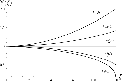
Figure 1: $\Upsilon_{-2}(\zeta)$, $\Upsilon_{-1}(\zeta)$, $\Upsilon_{0}^{\text{a}}(\zeta)$, $\Upsilon_{0}^{\text{b}}(\zeta)$ and $\Upsilon_{\ell}(\zeta)$ as functions of $\zeta$.

The direct term has not been found in closed form, but we now show how this can be achieved. Following Rajagopal and Kimball, Rajagopal and Kimball (1977) we write the direct term as the double integral

$$\varepsilon_{0}^{\text{a}}(\zeta)=-\frac{1}{8\pi^{3}}\int_{-\infty}^{\infty}\int_{0}^{\infty}\left[Q_{q/k_{\uparrow}}\left(\frac{u}{k_{\uparrow}}\right)+Q_{q/k_{\downarrow}}\left(\frac{u}{k_{\downarrow}}\right)\right]^{2}dq\,du,$$ (18)

where

$$Q_{q}(u)=\frac{\pi}{q}\left[q-\sqrt{\left(\frac{q}{2}-iu-1\right)\left(\frac{q}{2}-iu+1\right)}-\sqrt{\left(\frac{q}{2}+iu-1\right)\left(\frac{q}{2}+iu+1\right)}\right].$$ (19)

In the paramagnetic ($\zeta=0$) case, the transformation $s=q^{2}/4-u^{2}$ and $t=q\,u$ yields

$$\varepsilon_{0}^{\text{a}}(0)=-\frac{1}{2\pi}\int_{-\infty}^{\infty}\int_{0}^{\infty}\frac{1}{\sqrt{s^{2}+t^{2}}}\left[1-\left(\frac{\sqrt{(s-1)^{2}+t^{2}}+s-1}{\sqrt{s^{2}+t^{2}}+s}\right)^{1/2}\right]^{2}dt\,ds,$$ (20)

and, if we adopt polar coordinates, this becomes

$$\begin{split}\varepsilon_{0}^{\text{a}}(0)&=-\frac{1}{2\pi}\int_{0}^{\infty}\int_{0}^{\pi}\left[1-\sqrt{\frac{\sqrt{1-2r\cos\theta+r^{2}}-1+r\cos\theta}{r(1+\cos\theta)}}\right]^{2}d\theta\,dr\\ &=-\frac{1}{2\pi}\int_{0}^{\pi}\left[2\ln 2-(\pi-\theta)\tan\frac{\theta}{2}-2\tan^{2}\frac{\theta}{2}\ln\left(\sin\frac{\theta}{2}\right)\right]d\theta\\ &=\ln 2-1\\ &=-0.306853\ldots,\end{split}$$ (21)

which confirms Seidl’s numerical estimate Seidl (2004)

$$\varepsilon_{0}^{\text{a}}(0)=-0.30682\pm 0.00012.$$ (22)

In the ferromagnetic ($\zeta=1$) case, Eq. (18) yields

$$\varepsilon_{0}^{\text{a}}(1)=\frac{1}{2}\varepsilon_{0}^{\text{a}}(0)=\frac{\ln 2-1}{2}=-0.153426\ldots.$$ (23)

In intermediate cases, where $0<\zeta<1$, we define the spin-scaling function

$$\Upsilon_{0}^{\text{a}}(\zeta)=\frac{\varepsilon_{0}^{\text{a}}(\zeta)}{\varepsilon_{0}^{\text{a}}(0)},$$ (24)

and, from (18), we have

$$\Upsilon_{0}^{\text{a}}(\zeta)=\frac{1}{2}-\frac{1}{4\pi(\ln 2-1)}\int_{0}^{\infty}\int_{-1}^{1}P_{k_{\uparrow}}(r,z)P_{k_{\downarrow}}(r,z)\frac{i\,dz}{z}\,dr,$$ (25)

where

$$P_{k}(r,z)=1-\frac{\sqrt{rz-k^{2}}+\sqrt{r/z-k^{2}}}{\sqrt{r}\left(\sqrt{z}+1/\sqrt{z}\right)}.$$ (26)

Integrating over $r$ gives

$$\Upsilon_{0}^{\text{a}}(\zeta)=\frac{1}{2}-\frac{1}{4\pi(\ln 2-1)}\int_{-1}^{1}L_{k_{\uparrow},k_{\downarrow}}(z)\frac{i\,dz}{z},$$ (27)

where

$$\begin{split}L_{k_{\uparrow},k_{\downarrow}}(z)&=-k_{\uparrow}\ln k_{\uparrow}-k_{\downarrow}\ln k_{\downarrow}\\ &+\frac{1}{(z+1)^{2}}\Bigg{[}(zk_{\uparrow}-k_{\downarrow})^{2}\ln(zk_{\uparrow}-k_{\downarrow})+(zk_{\downarrow}-k_{\uparrow})^{2}\ln(zk_{\downarrow}-k_{\uparrow})\\ &-i\pi(k_{\downarrow}^{2}-2zk_{\uparrow}k_{\downarrow}+k_{\downarrow}^{2})+2z(k_{\uparrow}+k_{\downarrow})^{2}\ln(k_{\uparrow}+k_{\downarrow})-z(zk_{\uparrow}^{2}-2k_{\uparrow}k_{\downarrow}+zk_{\downarrow}^{2})\ln z\Bigg{]},\end{split}$$ (28)

and contour integration over $z$ eventually yields

$$\Upsilon_{0}^{\text{a}}(\zeta)=\frac{1}{2}+\frac{1-\zeta}{4(\ln 2-1)}\Bigg{[}2\ln 2-1-\sqrt{\frac{1+\zeta}{1-\zeta}}\\ +\frac{1+\zeta}{1-\zeta}\ln\left(1+\sqrt{\frac{1-\zeta}{1+\zeta}}\right)-\ln\left(1+\sqrt{\frac{1+\zeta}{1-\zeta}}\right)\Bigg{]}.$$ (29)

This is plotted in Fig. 1 and agrees well with Seidl’s approximation, Seidl (2004) deviating by a maximum of $0.0005$ near $\zeta=0.9815$.

In conclusion, we have shown that the energy of the high-density spin-polarized two-dimensional uniform electron gas can be found in closed form up to $O(r_{s})$. We believe that these new results, which are summarized in Table 1, will be useful in the future development of exchange-correlation functionals within density-functional theory.

We thank Prof. Stephen Taylor for helpful discussions. P.M.W.G. thanks the NCI National Facility for a generous grant of supercomputer time and the Australian Research Council (Grants DP0984806 and DP1094170) for funding.

Table 1: Energy coefficients and spin-scaling functions for 2-jellium in the high-density limit.

Term	Coefficient	$\varepsilon(0)$	$\varepsilon(1)$	$\Upsilon(\zeta)$
$r_{s}^{-2}$	$\varepsilon_{-2}(\zeta)$	$\displaystyle\frac{1}{2}$	$\displaystyle 1$	Eq. (5)
$r_{s}^{-1}$	$\varepsilon_{-1}(\zeta)$	$\displaystyle-\frac{4\sqrt{2}}{3\pi}$	$\displaystyle-\frac{8}{3\pi}$	Eq. (6)
$r_{s}^{0}$	$\varepsilon_{0}^{\text{a}}(\zeta)$	$\displaystyle\ln 2-1$	$\displaystyle\frac{\ln 2-1}{2}$	Eq. (29)
	$\varepsilon_{0}^{\text{b}}(\zeta)$	$\displaystyle\beta(2)-\frac{8}{\pi^{2}}\beta(4)$	$\displaystyle\beta(2)-\frac{8}{\pi^{2}}\beta(4)$	1
$r_{s}\ln r_{s}$	$\varepsilon_{\ell}(\zeta)$	$\displaystyle-\sqrt{2}\left(\frac{10}{3\pi}-1\right)$	$\displaystyle-\frac{1}{4}\left(\frac{10}{3\pi}-1\right)$	Eq. (12)